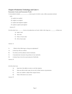
7
CHALLENGE
Technology Choice
at Home Versus
Abroad
economically efficient
minimizing the cost of
producing a specified
amount of output
184
Costs
An economist is a person who, when invited to give a talk at a banquet, tells
the audience there’s no such thing as a free lunch.
A manager of a semiconductor manufacturing firm, who can choose from many different production technologies, must determine whether the firm should use the same technology in its
foreign plant that it uses in its domestic plant. U.S. semiconductor manufacturing firms have
moved much of their production abroad since 1961, when Fairchild Semiconductor built a plant
in Hong Kong. According to the Semiconductor Industry Association (www.sia-online.org),
worldwide semiconductor April billings from the Americas dropped from 67% in 1976 to 30%
in 1990, and to 17% in 2010. Firms move their production abroad to benefit from lower taxes, lower
labor costs, and capital grants provided by foreign
governments to induce firms to move production to
their countries. Such grants can reduce the cost of
owning and operating an overseas semiconductor
fabrication facility by as much as 25% compared
with the costs of a U.S.-based plant.
The semiconductor manufacturer can produce
a chip using sophisticated equipment and relatively
few workers or many workers and less complex
equipment. In the United States, firms use a relatively capital-intensive technology, because doing
so minimizes their cost of producing a given level
of output. Will that same technology be cost minimizing if they move their production abroad?
A firm uses a two-step procedure in determining how to produce a certain amount
of output efficiently. It first determines which production processes are
technologically efficient so that it can produce the desired level of output with the
least amount of inputs. As we saw in Chapter 6, the firm uses engineering and other
information to determine its production function, which summarizes the many technologically efficient production processes available.
The firm’s second step is to pick from these technologically efficient production
processes the one that is also economically efficient, minimizing the cost of producing a specified amount of output. To determine which process minimizes its cost of
production, the firm uses information about the production function and the cost of
inputs.
By reducing its cost of producing a given level of output, a firm can increase its
profit. Any profit-maximizing competitive, monopolistic, or oligopolistic firm minimizes its cost of production.
7.1 The Nature of Costs
In this chapter, we
examine five main
topics
185
1. The Nature of Costs. When considering the cost of a proposed action, a good manager
of a firm takes account of forgone alternative opportunities.
2. Short-Run Costs. To minimize its costs in the short run, a firm adjusts its variable factors
(such as labor), but it cannot adjust its fixed factors (such as capital).
3. Long-Run Costs. In the long run, a firm adjusts all its inputs because usually all inputs
are variable.
4. Lower Costs in the Long Run. Long-run cost is as low as or lower than short-run cost
because the firm has more flexibility in the long run, technological progress occurs, and
workers and managers learn from experience.
5. Cost of Producing Multiple Goods. If the firm produces several goods simultaneously,
the cost of each may depend on the quantity of all the goods produced.
Businesspeople and economists need to understand the relationship between costs
of inputs and production to determine the least costly way to produce. Economists
have an additional reason for wanting to know about costs. As we’ll see in later
chapters, the relationship between output and costs plays an important role in determining the nature of a market—how many firms are in the market and how high
price is relative to cost.
7.1 The Nature of Costs
How much would it cost you to stand at the wrong end of a shooting gallery?
—S. J. Perelman
To show how a firm’s cost varies with its output, we first have to measure costs.
Businesspeople and economists often measure costs differently. Economists include
all relevant costs. To run a firm profitably, a manager must think like an economist
and consider all relevant costs. However, this same manager may direct the firm’s
accountant or bookkeeper to measure costs in ways that are more consistent with
tax laws and other laws so as to make the firm’s financial statements look good to
stockholders or to minimize the firm’s taxes.1
To produce a particular amount of output, a firm incurs costs for the required
inputs such as labor, capital, energy, and materials. A firm’s manager (or accountant) determines the cost of labor, energy, and materials by multiplying the price of
the factor by the number of units used. If workers earn $20 per hour and work a
total of 100 hours per day, then the firm’s cost of labor is
+20 * 100 = +2,000 per day. The manager can easily calculate these explicit costs,
which are its direct, out-of-pocket payments for inputs to its production process
within a given time period. While calculating explicit costs is straightforward, some
costs are implicit in that they reflect only a forgone opportunity rather than an
explicit, current expenditure. Properly taking account of forgone opportunities
requires particularly careful attention when dealing with durable capital goods, as
past expenditures for an input may be irrelevant to current cost calculations if that
input has no current, alternative use.
1See
“Tax Rules” in MyEconLab, Chapter 7.
186
CHAPTER 7 Costs
Opportunity Costs
economic cost or
opportunity cost
the value of the best alternative use of a resource
See Question 1.
APPLICATION
The Opportunity Cost
of an MBA
The economic cost or opportunity cost is the value of the best alternative use of a
resource. The economic or opportunity cost includes both explicit and implicit
costs. If a firm purchases and uses an input immediately, that input’s opportunity
cost is the amount the firm pays for it. However, if the firm does not use the input
in its production process, its best alternative would be to sell it to someone else at
the market price. The concept of an opportunity cost becomes particularly useful
when the firm uses an input that is not available for purchase in a market or that
was purchased in a market in the past.
An example of such an opportunity cost is the value of a manager’s time. For
instance, Maoyong owns and manages a firm. He pays himself only a small monthly
salary of $1,000 because he also receives the firm’s profit. However, Maoyong could
work for another firm and earn $11,000 a month. Thus, the opportunity cost of his
time is $11,000—from his best alternative use of his time—not the $1,000 he actually pays himself.
The classic example of an implicit opportunity cost is captured in the phrase
“There’s no such thing as a free lunch.” Suppose that your parents offer to take you
to lunch tomorrow. You know that they’ll pay for the meal, but you also know that
this lunch is not truly free. Your opportunity cost for the lunch is the best alternative use of your time. Presumably, the best alternative use of your time is studying
this textbook, but other possible alternatives include what you could earn at a job
or watching TV. Often such an opportunity is substantial.2 (What are you giving up
to study opportunity costs?)
During the sharp economic downturn in 2008–2010, did applications to MBA
programs fall, hold steady, or take off as tech stocks did during the first Internet
bubble? Knowledge of opportunity costs helps us answer this question.
For many potential students, the biggest cost of attending an MBA program
is the opportunity cost of giving up a well-paying job. Someone who leaves a
job that pays $5,000 per month to attend an MBA program is, in effect, incurring a $5,000-per-month opportunity cost, in addition to the tuition and cost
of textbooks (although this one is well worth the money).
Thus, it is not surprising that MBA applications rise in bad economic times
when outside opportunities decline. People thinking of going back to school
face a reduced opportunity cost of entering an MBA program if they think they
may be laid off or might not be promoted during an economic downturn. As
Stacey Kole, deputy dean for the MBA program at the University of Chicago
Graduate School of Business observed in 2008, “When there’s a go-go economy, fewer people decide to go back to school. When things go south the
opportunity cost of leaving work is lower.”
In 2008, when U.S. unemployment rose sharply and the economy was in
poor shape, the number of people seeking admission to MBA programs rose
sharply. The number of applicants to MBA programs in 2008 increased from
2007 by 79% in the United States, 77% in the United Kingdom, and 69% in
other European programs. In 2009, U.S. applications were up another 21%,
while those in Western Europe rose 72%.
2See
MyEconLab, Chapter 7, “Waiting for the Doctor.”
7.1 The Nature of Costs
SOLVED PROBLEM
7.1
187
Meredith’s firm sends her to a conference for managers and has paid her registration fee. Included in the registration fee is free admission to a class on how to
price derivative securities such as options. She is considering attending, but her
most attractive alternative opportunity is to attend a talk by Warren Buffett
about his investment strategies, which is scheduled at the same time. Although
she would be willing to pay $100 to hear his talk, the cost of a ticket is only $40.
Given that there are no other costs involved in attending either event, what is
Meredith’s opportunity cost of attending the derivatives talk?
Answer
See Question 2.
To calculate her opportunity cost, determine the benefit that Meredith would
forgo by attending the derivatives class. Because she incurs no additional fee to
attend the derivatives talk, Meredith’s opportunity cost is the forgone benefit of
hearing the Buffett speech. Because she values hearing the Buffett speech at $100,
but only has to pay $40, her net benefit from hearing that talk is
+60 (= +100 - +40). Thus, her opportunity cost of attending the derivatives
talk is $60.
Costs of Durable Inputs
durable good
a product that is usable
for years
Determining the opportunity cost of capital, such as land or equipment, requires
special considerations. Capital is a durable good: a product that is usable for years.
Two problems may arise in measuring the cost of capital. The first is how to allocate the initial purchase cost over time. The second is what to do if the value of the
capital changes over time.
We can avoid these two measurement problems if capital is rented instead of purchased. For example, suppose a firm can rent a small pick-up truck for $400 a
month or buy it outright for $20,000. If the firm rents the truck, the rental payment
is the relevant opportunity cost per month. The truck is rented month to month, so
the firm does not have to worry about how to allocate the purchase cost of a truck
over time. Moreover, the rental rate will adjust if the cost of trucks changes over
time. Thus, if the firm can rent capital for short periods of time, it calculates the cost
of this capital in the same way that it calculates the cost of nondurable inputs such
as labor services or materials.
The firm faces a more complex problem in determining the opportunity cost of
the truck if it purchases the truck. The firm’s accountant may expense the truck’s
purchase price by treating the full $20,000 as a cost at the time that the truck is purchased, or the accountant may amortize the cost by spreading the $20,000 over the
life of the truck, following rules set by an accounting organization or by a relevant
government authority such as the Internal Revenue Service (IRS).
A manager who wants to make sound decisions does not expense or amortize the
truck using such rules. The true opportunity cost of using a truck that the firm owns
is the amount that the firm could earn if it rented the truck to others. That is,
regardless of whether the firm rents or buys the truck, the manager views the opportunity cost of this capital good as the rental rate for a given period of time. If the
value of an older truck is less than that of a newer one, the rental rate for the truck
falls over time.
But what if there is no rental market for trucks available to the firm? It is still
important to determine an appropriate opportunity cost. Suppose that the firm has
two choices: It can choose not to buy the truck and keep the truck’s purchase price
of $20,000, or it can use the truck for a year and sell it for $17,000 at the end of
188
CHAPTER 7 Costs
See Question 3.
the year. If the firm does not purchase the truck, it will deposit the $20,000 in a
bank account that pays 5% per year, so the firm will have $21,000 at the end of the
year. Thus, the opportunity cost of capital of using the truck for a year is
+21,000 - +17,000 = +4,000.3 This $4,000 opportunity cost equals the $3,000
depreciation of the truck (= +20,000 - +17,000) plus the $1,000 in forgone interest that the firm could have earned over the year if the firm had invested the
$20,000.
Because the values of trucks, machines, and other equipment decline over time,
their rental rates fall, so the firm’s opportunity costs decline. In contrast, the value
of some land, buildings, and other forms of capital may rise over time. To maximize
profit, a firm must properly measure the opportunity cost of a piece of capital even
if its value rises over time. If a beauty parlor buys a building when similar buildings
in the area rent for $1,000 per month, the opportunity cost of using the building is
$1,000 a month. If land values increase so that rents in the area rise to $2,000 per
month, the beauty parlor’s opportunity cost of its building rises to $2,000 per
month.
Sunk Costs
sunk cost
a past expenditure that
cannot be recovered
An opportunity cost is not always easy to observe but should always be taken into
account when deciding how much to produce. In contrast, a sunk cost—a past
expenditure that cannot be recovered—though easily observed, is not relevant to a
manager when deciding how much to produce now. If an expenditure is sunk, it is
not an opportunity cost.4
If a firm buys a forklift for $25,000 and can resell it for the same price, it is not
a sunk expenditure, and the opportunity cost of the forklift is $25,000. If instead
the firm buys a specialized piece of equipment for $25,000 and cannot resell it, then
the original expenditure is a sunk cost. Because this equipment has no alternative
use and cannot be resold, its opportunity cost is zero, and it should not be included
in the firm’s current cost calculations. If the specialized equipment that originally
cost $25,000 can be resold for $10,000, then only $15,000 of the original expenditure is a sunk cost, and the opportunity cost is $10,000.
To illustrate why a sunk cost should not influence a manager’s current decisions,
consider a firm that paid $300,000 for a piece of land for which the market value
has fallen to $200,000. Now, the land’s true opportunity cost is $200,000. The
$100,000 difference between the $300,000 purchase price and the current market
value of $200,000 is a sunk cost that has already been incurred and cannot be recovered. The land is worth $240,000 to the firm if it builds a plant on this parcel. Is it
worth carrying out production on this land or should the land be sold for its market
value of $200,000? If the firm uses the original purchase price in its decision-making
process, the firm will falsely conclude that using the land for production will result
in a $60,000 loss: the $240,000 value of using the land minus the purchase price of
$300,000. Instead, the firm should use the land because it is worth $40,000 more as
a production facility than if the firm sells the land for $200,000, its next best alternative. Thus, the firm should use the land’s opportunity cost to make its decisions
and ignore the land’s sunk cost. In short, “There’s no use crying over spilt milk.”
3The
firm would also pay for gasoline, insurance, licensing fees, and other operating costs, but these
items would all be expensed as operating costs and would not appear in the firm’s accounts as capital costs.
4Nonetheless,
a sunk cost paid for a specialized input should still be deducted from income before
paying taxes even if that cost is sunk, and must therefore appear in financial accounts.
7.2 Short-Run Costs
189
7.2 Short-Run Costs
To make profit-maximizing decisions, a firm needs to know how its cost varies with
output. A firm’s cost rises as it increases its output. A firm cannot vary some of its
inputs, such as capital, in the short run (Chapter 6). As a result, it is usually more
costly for a firm to increase output in the short run than in the long run, when all
inputs can be varied. In this section, we look at the cost of increasing output in the
short run.
Short-Run Cost Measures
We start by using a numerical example to illustrate the basic cost concepts. We then
examine the graphic relationship between these concepts.
fixed cost (F )
a production expense that
does not vary with output
variable cost (VC )
a production expense that
changes with the quantity
of output produced
cost (total cost, C )
the sum of a firm’s variable cost and fixed cost:
C = VC + F.
Cost Levels To produce a given level of output in the short run, a firm incurs costs
for both its fixed and variable inputs. A firm’s fixed cost (F) is its production expense
that does not vary with output. The fixed cost includes the cost of inputs that the
firm cannot practically adjust in the short run, such as land, a plant, large machines,
and other capital goods. The fixed cost for a capital good a firm owns and uses is
the opportunity cost of not renting it to someone else. The fixed cost is $48 per day
for the firm in Table 7.1.
A firm’s variable cost (VC) is the production expense that changes with the quantity of output produced. The variable cost is the cost of the variable inputs—the
inputs the firm can adjust to alter its output level, such as labor and materials. Table
7.1 shows that the firm’s variable cost changes with output. Variable cost goes from
$25 a day when 1 unit is produced to $46 a day when 2 units are produced.
A firm’s cost (or total cost, C) is the sum of a firm’s variable cost and fixed cost:
C = VC + F.
The firm’s total cost of producing 2 units of output per day is $94 per day, which
is the sum of the fixed cost, $48, and the variable cost, $46. Because variable cost
Table 7.1 Variation of Short-Run Cost with Output
Output,
q
Fixed
Cost, F
Variable
Cost, VC
Total
Cost, C
Marginal
Cost, MC
Average Fixed
Cost, AFC ‫ ؍‬F/q
Average Variable
Cost, AVC ‫ ؍‬VC/q
Average Cost,
AC ‫ ؍‬C/q
0
1
48
0
48
48
25
73
25
48
25
73
2
48
46
94
21
24
23
47
3
4
48
66
114
20
16
22
38
48
82
130
16
12
20.5
32.5
5
48
100
148
18
9.6
20
29.6
6
48
120
168
20
8
20
28
7
48
141
189
21
6.9
20.1
27
8
48
168
216
27
6
21
27
9
48
198
246
30
5.3
22
27.3
10
48
230
278
32
4.8
23
27.8
11
48
272
320
42
4.4
24.7
29.1
12
48
321
369
49
4.0
26.8
30.8
190
CHAPTER 7 Costs
changes with the level of output, total cost also varies with the level of output, as
the table illustrates.
To decide how much to produce, a firm uses several measures of how its cost
varies with the level of output. Table 7.1 shows four such measures that we derive
using the fixed cost, the variable cost, and the total cost.
marginal cost (MC )
the amount by which a
firm’s cost changes if the
firm produces one more
unit of output
Marginal Cost A firm’s marginal cost (MC) is the amount by which a firm’s cost
changes if the firm produces one more unit of output. The marginal cost is5
MC =
∆C
,
∆q
where ∆C is the change in cost when output changes by ∆q. Table 7.1 shows that,
if the firm increases its output from 2 to 3 units, ∆q = 1, its total cost rises from
$94 to $114, ∆C = +20, so its marginal cost is +20 = ∆C/∆q.
Because only variable cost changes with output, we can also define marginal cost
as the change in variable cost from a one-unit increase in output:
MC =
See Question 4.
average fixed cost (AFC )
the fixed cost divided by
the units of output produced: AFC = F/q
average variable cost
(AVC )
the variable cost divided
by the units of output produced: AVC = VC/q
average cost (AC )
the total cost divided by
the units of output produced: AC = C/q
∆VC
.
∆q
As the firm increases output from 2 to 3 units, its variable cost increases by
∆VC = +20 = +66 - +46, so its marginal cost is MC = ∆VC/∆q = +20. A firm
uses marginal cost in deciding whether it pays to change its output level.
Average Costs Firms use three average cost measures. The average fixed cost
(AFC) is the fixed cost divided by the units of output produced: AFC = F/q. The
average fixed cost falls as output rises because the fixed cost is spread over more
units. The average fixed cost falls from $48 for 1 unit of output to $4 for 12 units
of output in Table 7.1.
The average variable cost (AVC) is the variable cost divided by the units of output produced: AVC = VC/q. Because the variable cost increases with output, the
average variable cost may either increase or decrease as output rises. The average
variable cost is $25 at 1 unit, falls until it reaches a minimum of $20 at 6 units, and
then rises. As we show in Chapter 8, a firm uses the average variable cost to determine whether to shut down operations when demand is low.
The average cost (AC)—or average total cost—is the total cost divided by the
units of output produced: AC = C/q. The average cost is the sum of the average
fixed cost and the average variable cost:6
AC = AFC + AVC.
See Questions 5 and 6.
In Table 7.1, as output increases, average cost falls until output is 8 units and
then rises. The firm makes a profit if its average cost is below its price, which is the
firm’s average revenue.7
5If
we use calculus, the marginal cost is MC = dC(q)/dq, where C(q) is the cost function that shows
how cost varies with output. The calculus definition says how cost changes for an infinitesimal
change in output. To illustrate the idea, however, we use larger changes in the table.
6Because
C = VC + F, if we divide both sides of the equation by q, we obtain
AC = C/q = F/q + VC/q = AFC + AVC.
7See
MyEconLab, Chapter 7, “Lowering Transaction Costs for Used Goods at eBay and AbeBooks,”
for a discussion of transaction, fixed, and variable shopping costs for consumers.
7.2 Short-Run Costs
191
Short-Run Cost Curves
We illustrate the relationship between output and the various cost measures using
curves in Figure 7.1. Panel a shows the variable cost, fixed cost, and total cost curves
that correspond to Table 7.1. The fixed cost, which does not vary with output, is a
horizontal line at $48. The variable cost curve is zero at zero units of output and
rises with output. The total cost curve, which is the vertical sum of the variable cost
curve and the fixed cost line, is $48 higher than the variable cost curve at every output level, so the variable cost and total cost curves are parallel.
Panel b shows the average fixed cost, average variable cost, average cost, and
marginal cost curves. The average fixed cost curve falls as output increases. It
Figure 7.1 Short-Run Cost Curves
Cost, $
(a)
400
C
VC
A
216
27
1
1
48
0
20
B
120
F
2
4
6
8
(b)
Cost per unit, $
(a) Because the total cost differs from
the variable cost by the fixed cost, F,
of $48, the total cost curve, C, is parallel to the variable cost curve, VC. (b)
The marginal cost curve, MC, cuts the
average variable cost, AVC, and average cost, AC, curves at their minimums. The height of the AC curve at
point a equals the slope of the line
from the origin to the cost curve at A.
The height of the AVC at b equals the
slope of the line from the origin to the
variable cost curve at B. The height of
the marginal cost is the slope of either
the C or VC curve at that quantity.
10
Quantity, q, Units per day
60
MC
28
27
a
b
20
AC
AVC
8
AFC
0
2
4
6
10
8
Quantity, q, Units per day
192
CHAPTER 7 Costs
See Questions 7 and 8 and
Problems 26–29.
approaches zero as output gets large because the fixed cost is spread over many
units of output. The average cost curve is the vertical sum of the average fixed cost
and average variable cost curves. For example, at 6 units of output, the average variable cost is 20 and the average fixed cost is 8, so the average cost is 28.
The relationships between the average and marginal curves to the total curves are
similar to those between the total product, marginal product, and average product
curves, which we discussed in Chapter 6. The average cost at a particular output
level is the slope of a line from the origin to the corresponding point on the cost
curve. The slope of that line is the rise—the cost at that output level—divided by the
run—the output level—which is the definition of the average cost. In panel a, the
slope of the line from the origin to point A is the average cost for 8 units of output.
The height of the cost curve at A is 216, so the slope is 216/8 = 27, which is the
height of the average cost curve at the corresponding point a in panel b.
Similarly, the average variable cost is the slope of a line from the origin to a point
on the variable cost curve. The slope of the dashed line from the origin to B in panel
a is 20—the height of the variable cost curve, 120, divided by the number of units
of output, 6—which is the height of the average variable cost at 6 units of output,
point b in panel b.
The marginal cost is the slope of either the cost curve or the variable cost curve
at a given output level. As the cost and variable cost curves are parallel, they have
the same slope at any given output. The difference between cost and variable cost is
fixed cost, which does not affect marginal cost.
The dashed line from the origin is tangent to the cost curve at A in panel a. Thus,
the slope of the dashed line equals both the average cost and the marginal cost at 8
units of output. This equality occurs at the corresponding point a in panel b, where
the marginal cost curve intersects the average cost. (See Appendix 7A for a mathematical proof.)
Where the marginal cost curve is below the average cost, the average cost curve
declines with output. Because the average cost of 47 for 2 units is greater than the
marginal cost of the third unit, 20, the average cost for 3 units falls to 38. Where
the marginal cost is above the average cost, the average cost curve rises with output.
At 8 units, the marginal cost equals the average cost, so the average is unchanging,
which is the minimum point, a, of the average cost curve.
We can show the same results using the graph. Because the dashed line from the
origin is tangent to the variable cost curve at B in panel a, the marginal cost equals
the average variable cost at the corresponding point b in panel b. Again, where
marginal cost is above average variable cost, the average variable cost curve rises
with output; where marginal cost is below average variable cost, the average variable cost curve falls with output. Because the average cost curve is above the average variable cost curve everywhere and the marginal cost curve is rising where it
crosses both average curves, the minimum of the average variable cost curve, b, is
at a lower output level than the minimum of the average cost curve, a.
Production Functions and the Shape of Cost Curves
The production function determines the shape of a firm’s cost curves. The production function shows the amount of inputs needed to produce a given level of output.
The firm calculates its cost by multiplying the quantity of each input by its price and
summing the costs of the inputs.
If a firm produces output using capital and labor, and its capital is fixed in the
short run, the firm’s variable cost is its cost of labor. Its labor cost is the wage per
hour, w, times the number of hours of labor, L, employed by the firm: VC = wL.
7.2 Short-Run Costs
193
In the short run, when the firm’s capital is fixed, the only way the firm can
increase its output is to use more labor. If the firm increases its labor enough, it
reaches the point of diminishing marginal return to labor, at which each extra
worker increases output by a smaller amount. We can use this information about
the relationship between labor and output—the production function—to determine
the shape of the variable cost curve and its related curves.
Shape of the Variable Cost Curve If input prices are constant, the production
function determines the shape of the variable cost curve. We illustrate this relationship for the firm in Figure 7.2. The firm faces a constant input price for labor, the
wage, of $5 per hour.
The total product of labor curve in Figure 7.2 shows the firm’s short-run production function relationship between output and labor when capital is held fixed. For
example, it takes 24 hours of labor to produce 6 units of output. Nearly doubling
labor to 46 hours causes output to increase by only two-thirds to 10 units of output. As labor increases, the total product of labor curve increases less than in proportion. This flattening of the total product of labor curve at higher levels of labor
reflects the diminishing marginal return to labor.
This curve shows both the production relation of output to labor and the variable
cost relation of output to cost. Because each hour of work costs the firm $5, we can
relabel the horizontal axis in Figure 7.2 to show the firm’s variable cost, which is its
cost of labor. To produce 6 units of output takes 24 hours of labor, so the firm’s variable cost is $120. By using the variable cost labels on the horizontal axis, the total
product of labor curve becomes the variable cost curve, where each worker costs the
Figure 7.2 Variable Cost and Total Product of Labor
Quantity, q, Units per day
The firm’s short-run variable cost curve and its total
product of labor curve have the same shape. The total
product of labor curve uses the horizontal axis measuring
hours of work. The variable cost curve uses the horizontal axis measuring labor cost, which is the only variable
cost.
Total product of labor,
Variable cost
13
10
6
5
1
0
5
25
20 24
100 120
46
230
77
385
L, Hours of labor per day
VC = wL, Variable cost, $
194
CHAPTER 7 Costs
See Question 9 and
Problem 30.
firm $120 per day in wages. The variable cost curve in Figure 7.2 is the same as the
one in panel a of Figure 7.1, in which the output and cost axes are reversed. For
example, the variable cost of producing 6 units is $120 in both figures.
Diminishing marginal returns in the production function cause the variable cost
to rise more than in proportion as output increases. Because the production function determines the shape of the variable cost curve, it also determines the shape of
the marginal, average variable, and average cost curves. We now examine the shape
of each of these cost curves in detail because in making decisions, firms rely more
on these per-unit cost measures than on total variable cost.
Shape of the Marginal Cost Curve The marginal cost is the change in variable
cost as output increases by one unit: MC = ∆VC/∆q. In the short run, capital is
fixed, so the only way the firm can produce more output is to use extra labor. The
extra labor required to produce one more unit of output is ∆L/∆q. The extra labor
costs the firm w per unit, so the firm’s cost rises by w(∆L/∆q). As a result, the firm’s
marginal cost is
MC =
∆VC
∆L
= w
.
∆q
∆q
The marginal cost equals the wage times the extra labor necessary to produce one
more unit of output. To increase output by one unit from 5 to 6 units takes 4 extra
workers in Figure 7.2. If the wage is $5 per hour, the marginal cost is $20.
How do we know how much extra labor we need to produce one more unit of
output? That information comes from the production function. The marginal product of labor—the amount of extra output produced by another unit of labor, holding other inputs fixed—is MPL = ∆q/∆L. Thus, the extra labor we need to produce
one more unit of output, ∆L/∆q, is 1/MPL, so the firm’s marginal cost is
MC =
w
.
MPL
(7.1)
Equation 7.1 says that the marginal cost equals the wage divided by the marginal
product of labor. If the firm is producing 5 units of output, it takes 4 extra hours of
labor to produce 1 more unit of output in Figure 7.2, so the marginal product of an
hour of labor is 14. Given a wage of $5 an hour, the marginal cost of the sixth
unit is $5 divided by 14, or $20, as panel b of Figure 7.1 shows.
Equation 7.1 shows that the marginal cost moves in the direction opposite that
of the marginal product of labor. At low levels of labor, the marginal product of
labor commonly rises with additional labor because extra workers help the original
workers and they can collectively make better use of the firm’s equipment (Chapter
6). As the marginal product of labor rises, the marginal cost falls.
Eventually, however, as the number of workers increases, workers must share the
fixed amount of equipment and may get in each other’s way, so the marginal cost
curve slopes upward because of diminishing marginal returns to labor. Thus, the
marginal cost first falls and then rises, as panel b of Figure 7.1 illustrates.
Shape of the Average Cost Curves Diminishing marginal returns to labor, by
determining the shape of the variable cost curve, also determine the shape of the
average variable cost curve. The average variable cost is the variable cost divided by
output: AVC = VC/q. For the firm we’ve been examining, whose only variable
input is labor, variable cost is wL, so average variable cost is
AVC =
VC
wL
=
.
q
q
7.2 Short-Run Costs
195
Because the average product of labor is q/L, average variable cost is the wage
divided by the average product of labor:
AVC =
APPLICATION
Short-Run Cost
Curves for a Furniture
Manufacturer
(7.2)
In Figure 7.2, at 6 units of output, the average product of labor is 14 (= q/L = 6/24),
so the average variable cost is $20, which is the wage, $5, divided by the average
product of labor, 14.
With a constant wage, the average variable cost moves in the opposite direction
of the average product of labor in Equation 7.2. As we discussed in Chapter 6, the
average product of labor tends to rise and then fall, so the average cost tends to fall
and then rise, as in panel b of Figure 7.1.
The average cost curve is the vertical sum of the average variable cost curve and
the average fixed cost curve, as in panel b. If the average variable cost curve is
U-shaped, adding the strictly falling average fixed cost makes the average cost fall
more steeply than the average variable cost curve at low output levels. At high output levels, the average cost and average variable cost curves differ by ever smaller
amounts, as the average fixed cost, F/q, approaches zero. Thus, the average cost
curve is also U-shaped.
The short-run average cost curve for a U.S. furniture manufacturer is Ushaped, even though its average variable cost is strictly upward sloping. The
graph (based on the estimates of Hsieh, 1995) shows the firm’s various shortrun cost curves, where the firm’s capital is fixed at K = 100. Appendix 7B
derives the firm’s short-run cost curves mathematically.
The firm’s average fixed cost (AFC) falls as output increases. The firm’s
average variable cost curve is strictly increasing. The average cost (AC) curve
is the vertical sum of the average variable cost (AVC) and average fixed cost
curves. Because the average fixed cost curve falls with output and the average
variable cost curve rises with output, the average cost curve is U-shaped. The
firm’s marginal cost (MC) lies above the rising average variable cost curve for
all positive quantities of output and cuts the average cost curve at its minimum.
Costs per unit, $
See Problems 31 and 32.
w
.
APL
50
MC
40
30
AC
AVC
20
10
AFC
0
100
200
300
q, Units per year
196
CHAPTER 7 Costs
Effects of Taxes on Costs
Taxes applied to a firm shift some or all of the marginal and average cost curves.
For example, suppose that the government collects a specific tax of $10 per unit of
output from the firm. This tax, which varies with output, affects the firm’s variable
cost but not its fixed cost. As a result, it affects the firm’s average cost, average variable cost, and marginal cost curves but not its average fixed cost curve.
At every quantity, the average variable cost and the average cost rise by the full
amount of the tax. The second column of Table 7.2 (based on Table 7.1) shows the
firm’s average variable cost before the tax, AVC b. For example, if it sells 6 units of
output, its average variable cost is $20. After the tax, the firm must pay the government $10 per unit, so the firm’s after-tax average variable cost rises to $30. More
generally, the firm’s after-tax average variable cost, AVC a, is its average variable cost
of production—the before-tax average variable cost—plus the tax per unit, $10:
AVC a = AVC b + +10.
The average cost equals the average variable cost plus the average fixed cost.
Because the tax increases average variable cost by $10 and does not affect the average fixed cost, the tax increases average cost by $10.
The tax also increases the firm’s marginal cost. Suppose that the firm wants to
increase output from 7 to 8 units. The firm’s actual cost of producing the eighth
unit—its before-tax marginal cost, MC b :is $27. To produce an extra unit of output, the cost to the firm is the marginal cost of producing the extra unit plus $10,
so its after-tax marginal cost is MC a = MC b + +10. In particular, its after-tax
marginal cost of producing the eighth unit is $37.
A specific tax shifts the marginal cost and the average cost curves upward in
Figure 7.3 by the amount of the tax, $10 per unit. The after-tax marginal cost intersects the after-tax average cost at its minimum. Because both the marginal and average cost curves shift upward by exactly the same amount, the after-tax average cost
curve reaches its minimum at the same level of output, 8 units, as the before-tax
average cost, as Figure 7.3 shows. At 8 units, the minimum of the before-tax average cost curve is $27 and that of the after-tax average cost curve is $37. So even
though a specific tax increases a firm’s average cost, it does not affect the output at
which average cost is minimized.
Table 7.2 Effect of a Specific Tax of $10 per Unit on Short-Run Costs
Q
AVC b
AVC a ‫ ؍‬AVC b ؉ +10
AC b ‫ ؍‬C/q
AC a ‫ ؍‬C/q ؉ +10
MC b
MC a ‫ ؍‬MC b ؉ +10
1
25
35
73
83
25
35
2
23
33
47
57
21
31
3
22
32
38
48
20
30
4
20.5
30.5
32.5
42.5
16
26
5
20
30
29.6
39.6
18
28
6
20
30
28
38
20
30
7
20.1
30.1
27
37
21
31
8
21
31
27
37
27
37
9
22
32
27.3
37.3
30
40
10
23
33
27.8
37.8
32
42
11
24.7
34.7
29.1
39.1
42
52
12
26.8
36.8
30.8
40.8
49
59
7.2 Short-Run Costs
197
A specific tax of $10 per unit
shifts both the marginal cost
and average cost curves upward
by $10. Because of the parallel
upward shift of the average cost
curve, the minimum of both the
before-tax average cost curve,
AC b, and the after-tax average
cost curve, AC a, occurs at the
same output, 8 units.
Costs per unit, $
Figure 7.3 Effect of a Specific Tax on Cost Curves
MC a = MC b + 10
80
MC b
$10
37
AC a = AC b + 10
$10
AC b
27
0
5
8
10
15
q, Units per day
Similarly, we can analyze the effect of a franchise tax on costs. A franchise tax—
also called a business license fee—is a lump sum that a firm pays for the right to
operate a business. An $800-per-year tax is levied “for the privilege of doing business in California.” A one-year license to sell hot dogs from two stands in front of
New York City’s Metropolitan Museum of Art cost $642,701 in 2009. These taxes
do not vary with output, so they affect firms’ fixed costs only—not their variable
costs.
SOLVED PROBLEM
7.2
What is the effect of a lump-sum franchise tax ᏸ on the quantity at which a firm’s
after-tax average cost curve reaches its minimum? (Assume that the firm’s beforetax average cost curve is U-shaped.)
Answer
1. Determine the average tax per unit of output. Because the franchise tax is a
lump-sum payment that does not vary with output, the more the firm produces, the less tax it pays per unit. The tax per unit is бЏё/q. If the firm sells only
1 unit, its cost is бЏё; however, if it sells 100 units, its tax payment per unit is
only бЏё/100.
2. Show how the tax per unit affects the average cost. The firm’s after-tax average cost, AC a, is the sum of its before-tax average cost, AC b, and its average
tax payment per unit, бЏё/q. Because the average tax payment per unit falls with
output, the gap between the after-tax average cost curve and the before-tax
average cost curve also falls with output on the graph.
CHAPTER 7 Costs
Costs per unit, $
198
MC
AC a = AC b + бЏё/q
бЏё/q
AC b
qb
qa
q, Units per day
3. Determine the effect of the tax on the marginal cost curve. Because the fran-
chise tax does not vary with output, it does not affect the marginal cost curve.
4. Compare the minimum points of the two average cost curves. The marginal
cost curve crosses from below both average cost curves at their minimum
points. Because the after-tax average cost lies above the before-tax average
cost curve, the quantity at which the after-tax average cost curve reaches its
minimum, qa, is larger than the quantity, qb, at which the before-tax average
cost curve achieves a minimum.
See Question 10.
Short-Run Cost Summary
We discussed three cost-level curves—total cost, fixed cost, and variable cost—and
four cost-per-unit curves—average cost, average fixed cost, average variable cost,
and marginal cost. Understanding the shapes of these curves and the relationships
between them is crucial to understanding the analysis of firm behavior in the rest of
this book. Fortunately, we can derive most of what we need to know about the
shapes and the relationships between the curves using four basic concepts:
в– в– в– в– In the short run, the cost associated with inputs that cannot be adjusted is fixed,
while the cost from inputs that can be adjusted is variable.
Given that input prices are constant, the shapes of the variable cost and cost
curves are determined by the production function.
Where there are diminishing marginal returns to a variable input, the variable
cost and cost curves become relatively steep as output increases, so the average
cost, average variable cost, and marginal cost curves rise with output.
Because of the relationship between marginals and averages, both the average
cost and average variable cost curves fall when marginal cost is below them and
rise when marginal cost is above them, so the marginal cost cuts both these average cost curves at their minimum points.
7.3 Long-Run Costs
199
7.3 Long-Run Costs
In the long run, the firm adjusts all its inputs so that its cost of production is as low
as possible. The firm can change its plant size, design and build new machines, and
otherwise adjust inputs that were fixed in the short run.
Although firms may incur fixed costs in the long run, these fixed costs are
avoidable (rather than sunk, as in the short run). The rent of F per month that a
restaurant pays is a fixed cost because it does not vary with the number of meals
(output) served. In the short run, this fixed cost is sunk: The firm must pay F even
if the restaurant does not operate. In the long run, this fixed cost is avoidable: The
firm does not have to pay this rent if it shuts down. The long run is determined by
the length of the rental contract during which time the firm is obligated to pay rent.
In our examples throughout this chapter, we assume that all inputs can be varied
in the long run so that there are no long-run fixed costs (F = 0). As a result, the longrun total cost equals the long-run variable cost: C = VC. Thus, our firm is concerned
about only three cost concepts in the long run—total cost, average cost, and marginal
cost—instead of the seven cost concepts that it considers in the short run.
To produce a given quantity of output at minimum cost, our firm uses information about the production function and the price of labor and capital. The firm
chooses how much labor and capital to use in the long run, whereas the firm
chooses only how much labor to use in the short run when capital is fixed. As a consequence, the firm’s long-run cost is lower than its short-run cost of production if it
has to use the “wrong” level of capital in the short run. In this section, we show
how a firm picks the cost-minimizing combinations of inputs in the long run.
Input Choice
A firm can produce a given level of output using many different technologically efficient combinations of inputs, as summarized by an isoquant (Chapter 6). From
among the technologically efficient combinations of inputs, a firm wants to choose
the particular bundle with the lowest cost of production, which is the economically
efficient combination of inputs. To do so, the firm combines information about
technology from the isoquant with information about the cost of labor and capital.
We now show how information about cost can be summarized in an isocost line.
Then we show how a firm can combine the information in an isoquant and isocost
lines to pick the economically efficient combination of inputs.
Isocost Line The cost of producing a given level of output depends on the price of
labor and capital. The firm hires L hours of labor services at a wage of w per hour,
so its labor cost is wL. The firm rents K hours of machine services at a rental rate
of r per hour, so its capital cost is rK. (If the firm owns the capital, r is the implicit
rental rate.) The firm’s total cost is the sum of its labor and capital costs:
C = wL + rK.
isocost line
all the combinations of
inputs that require the
same (iso) total expenditure (cost)
(7.3)
The firm can hire as much labor and capital as it wants at these constant input
prices.
The firm can use many combinations of labor and capital that cost the same
amount. Suppose that the wage rate, w, is $5 an hour and the rental rate of capital,
r, is $10. Five of the many combinations of labor and capital that the firm can use
that cost $100 are listed in Table 7.3. These combinations of labor and capital are
plotted on an isocost line, which is all the combinations of inputs that require the
same (iso) total expenditure (cost). Figure 7.4 shows three isocost lines. The $100
200
CHAPTER 7 Costs
Table 7.3 Bundles of Labor and Capital That Cost the Firm $100
Bundle
Labor,
L
Capital,
K
a
20
0
b
14
3
c
10
d
6
e
0
Labor Cost,
wL ‫ ؍‬+5L
Capital Cost,
rK ‫ ؍‬+10K
Total Cost,
wL Ш‰ rK
$100
$0
$100
$70
$30
$100
5
$50
$50
$100
7
$30
$70
$100
10
$0
$100
$100
Figure 7.4 A Family of Isocost Lines
K, Units of capital per year
An isocost line shows all the combinations of labor and
capital that cost the firm the same amount. The greater
the total cost, the farther from the origin the isocost lies.
All the isocosts have the same slope, ПЄw/r = ПЄ 12. The
15 =
$150
$10
10 =
$100
$10
slope shows the rate at which the firm can substitute capital for labor holding total cost constant: For each extra
unit of capital it uses, the firm must use two fewer units
of labor to hold its cost constant.
e
d
5=
$50
$10
c
b
$50 isocost
$100 isocost
$150 isocost
a
$100
= 20
$5
$50
= 10
$5
$150
= 30
$5
L, Units of labor per year
isocost line represents all the combinations of labor and capital that the firm can
buy for $100, including the combinations a through e in Table 7.3.
Along an isocost line, cost is fixed at a particular level, C, so by setting cost at C
in Equation 7.3, we can write the equation for the C isocost line as
C = wL + rK.
Using algebra, we can rewrite this equation to show how much capital the firm can
buy if it spends a total of C and purchases L units of labor:
K =
C
w
- L.
r
r
(7.4)
7.3 Long-Run Costs
201
By substituting C = +100, w = +5, and r = +10 in Equation 7.4, we find that the
$100 isocost line is K = 10 - 12 2L. We can use Equation 7.4 to derive three properties of isocost lines.
First, where the isocost lines hit the capital and labor axes depends on the firm’s
cost, C, and on the input prices. The C isocost line intersects the capital axis where
the firm is using only capital. Setting L = 0 in Equation 7.4, we find that the firm
buys K = C/r units of capital. In the figure, the $100 isocost line intersects the capital axis at +100/+10 = 10 units of capital. Similarly, the intersection of the isocost
line with the labor axis is at C/w, which is the amount of labor the firm hires if it
uses only labor. In the figure, the intersection of the $100 isocost line with the labor
axis occurs at L = 20, where K = 10 - 12 * 20 = 0.
Second, isocosts that are farther from the origin have higher costs than those that
are closer to the origin. Because the isocost lines intersect the capital axis at C/r and
the labor axis at C/w, an increase in the cost shifts these intersections with the axes
proportionately outward. The $50 isocost line hits the capital axis at 5 and the labor
axis at 10, whereas the $100 isocost line intersects at 10 and 20.
Third, the slope of each isocost line is the same. From Equation 7.4, if the firm
increases labor by ∆L, it must decrease capital by
w
∆K = Ϫ ∆L.
r
Dividing both sides of this expression by ∆L, we find that the slope of an isocost
line, ∆K/∆L, is Ϫw/r. Thus, the slope of the isocost line depends on the relative
prices of the inputs. The slope of the isocost lines in the figure is
Ϫw/r = Ϫ +5/+10 = Ϫ 12. If the firm uses two more units of labor, ∆L = 2, it must
reduce capital by one unit, ∆K = Ϫ 12 ∆L = Ϫ1, to keep its total cost constant.
Because all isocost lines are based on the same relative prices, they all have the same
slope, so they are parallel.
The isocost line plays a similar role in the firm’s decision making as the budget
line does in consumer decision making. Both an isocost line and a budget line are
straight lines whose slopes depend on relative prices. There is an important difference between them, however. The consumer has a single budget line determined by
the consumer’s income. The firm faces many isocost lines, each of which corresponds to a different level of expenditures the firm might make. A firm may incur a
relatively low cost by producing relatively little output with few inputs, or it may
incur a relatively high cost by producing a relatively large quantity.
Combining Cost and Production Information By combining the information
about costs contained in the isocost lines with information about efficient production summarized by an isoquant, a firm chooses the lowest-cost way to produce a
given level of output. We examine how our furniture manufacturer picks the combination of labor and capital that minimizes its cost of producing 100 units of output. Figure 7.5 shows the isoquant for 100 units of output (based on Hsieh, 1995)
and the isocost lines where the rental rate of a unit of capital is $8 per hour and the
wage rate is $24 per hour.
The firm can choose any of three equivalent approaches to minimize its cost:
в– в– в– Lowest-isocost rule. Pick the bundle of inputs where the lowest isocost line
touches the isoquant.
Tangency rule. Pick the bundle of inputs where the isoquant is tangent to the isocost line.
Last-dollar rule. Pick the bundle of inputs where the last dollar spent on one input
gives as much extra output as the last dollar spent on any other input.
202
CHAPTER 7 Costs
Figure 7.5 Cost Minimization
K, Units of capital per hour
The furniture manufacturer minimizes its cost of producing 100 units of output by producing at x (L = 50 and
K = 100). This cost-minimizing combination of inputs is
determined
by
the
tangency
between
the
q = 100 isoquant and the lowest isocost line, $2,000,
that touches that isoquant. At x, the isocost is tangent to
the isoquant, so the slope of the isocost, ПЄw/r = ПЄ3,
equals the slope of the isoquant, which is the negative of
the marginal rate of technical substitution. That is, the
rate at which the firm can trade capital for labor in the
input markets equals the rate at which it can substitute
capital for labor in the production process.
q = 100 isoquant
$3,000
isocost
y
303
$2,000
isocost
$1,000
isocost
x
100
z
28
0
24
50
116
L, Units of labor per hour
Using the lowest-isocost rule, the firm minimizes its cost by using the combination of inputs on the isoquant that is on the lowest isocost line that touches the isoquant. The lowest possible isoquant that will allow the furniture manufacturer to
produce 100 units of output is tangent to the $2,000 isocost line. This isocost line
touches the isoquant at the bundle of inputs x, where the firm uses L = 50 workers
and K = 100 units of capital.
How do we know that x is the least costly way to produce 100 units of output?
We need to demonstrate that other practical combinations of input produce less
than 100 units or produce 100 units at greater cost.
If the firm spent less than $2,000, it could not produce 100 units of output. Each
combination of inputs on the $1,000 isocost line lies below the isoquant, so the firm
cannot produce 100 units of output for $1,000.
The firm can produce 100 units of output using other combinations of inputs
beside x; however, using these other bundles of inputs is more expensive. For example, the firm can produce 100 units of output using the combinations
y (L = 24, K = 303) or z (L = 116, K = 28). Both these combinations, however,
cost the firm $3,000.
7.3 Long-Run Costs
203
If an isocost line crosses the isoquant twice, as the $3,000 isocost line does, there
must be another lower isocost line that also touches the isoquant. The lowest possible isocost line that touches the isoquant, the $2,000 isocost line, is tangent to the
isoquant at a single bundle, x. Thus, the firm may use the tangency rule: The firm
chooses the input bundle where the relevant isoquant is tangent to an isocost line to
produce a given level of output at the lowest cost.
We can interpret this tangency or cost minimization condition in two ways. At
the point of tangency, the slope of the isoquant equals the slope of the isocost. As
we showed in Chapter 6, the slope of the isoquant is the marginal rate of technical
substitution (MRTS). The slope of the isocost is the negative of the ratio of the wage
to the cost of capital, ПЄw/r. Thus, to minimize its cost of producing a given level of
output, a firm chooses its inputs so that the marginal rate of technical substitution
equals the negative of the relative input prices:
w
MRTS = ПЄ .
r
(7.5)
The firm picks inputs so that the rate at which it can substitute capital for labor in
the production process, the MRTS, exactly equals the rate at which it can trade capital for labor in input markets, ПЄw/r.
The furniture manufacturer’s marginal rate of technical substitution is Ϫ1.5K/L.
At K = 100 and L = 50, its MRTS is ПЄ3, which equals the negative of the ratio of
the input prices it faces, ПЄw/r = ПЄ24/8 = ПЄ3. In contrast, at y, the isocost cuts
the isoquant so the slopes are not equal. At y, the MRTS is ПЄ18.9375, which is
greater than the ratio of the input price, 3. Because the slopes are not equal at y, the
firm can produce the same output at lower cost. As the figure shows, the cost of producing at y is $3,000, whereas the cost of producing at x is only $2,000.
We can interpret the condition in Equation 7.5 in another way. We showed in
Chapter 6 that the marginal rate of technical substitution equals the negative of the
ratio of the marginal product of labor to that of capital: MRTS = ПЄMPL/MPK.
Thus, the cost-minimizing condition in Equation 7.5 (taking the absolute value of
both sides) is
MPL
w
= .
r
MPK
(7.6)
This expression may be rewritten as
MPL
MPK
=
.
w
r
(7.7)
Equation 7.7 states the last-dollar rule: Cost is minimized if inputs are chosen so
that the last dollar spent on labor adds as much extra output as the last dollar spent
on capital.
The furniture firm’s marginal product of labor is MPL = 0.6q/L, and its marginal
product of capital is MPK = 0.4q/K.8 At Bundle x, the furniture firm’s marginal
product of labor is 1.2(= 0.6 * 100/50) and its marginal product of capital is 0.4.
The last dollar spent on labor gets the firm
MPL
1.2
=
= 0.05
w
24
furniture manufacturer’s production function, q = 1.52L0.6K 0.4, is a Cobb-Douglas production
function. The marginal product formula for Cobb-Douglas production functions is derived in
Appendix 6B.
8The
204
CHAPTER 7 Costs
more output. The last dollar spent on capital also gets the firm
MPK
0.4
= 0.05
=
r
8
extra output. Thus, spending one more dollar on labor at x gets the firm as much
extra output as spending the same amount on capital. Equation 7.6 holds, so the
firm is minimizing its cost of producing 100 units of output.
If instead the firm produced at y, where it is using more capital and less labor, its
MPL is 2.5(= 0.6 * 100/24) and the MPK is approximately 0.13 (L0.4 * 100/303).
As a result, the last dollar spent on labor gets MPL/w L 0.1 more unit of output,
whereas the last dollar spent on capital gets only a fourth as much extra output,
MPK/r L 0.017. At y, if the firm shifts one dollar from capital to labor, output falls
by 0.017 because there is less capital but also increases by 0.1 because there is more
labor for a net gain of 0.083 more output at the same cost. The firm should shift
even more resources from capital to labor—which increases the marginal product of
capital and decreases the marginal product of labor—until Equation 7.6 holds with
equality at x.
To summarize, we demonstrated that there are three equivalent rules that the firm
can use to pick the lowest-cost combination of inputs to produce a given level of
output when isoquants are smooth: the lowest-isocost rule, the tangency rule
(Equations 7.5 and 7.6), and the last-dollar rule (Equation 7.7). If the isoquant is
not smooth, the lowest-cost method of production cannot be determined by using
the tangency rule or the last-dollar rule. The lowest-isocost rule always works—even
when isoquants are not smooth—as MyEconLab, Chapter 7, “Rice Milling on
Java,” illustrates.
Factor Price Changes Once the furniture manufacturer determines the lowestcost combination of inputs to produce a given level of output, it uses that method
as long as the input prices remain constant. How should the firm change its behavior if the cost of one of the factors changes? Suppose that the wage falls from $24
to $8 but the rental rate of capital stays constant at $8.
The firm minimizes its new cost by substituting away from the now relatively
more expensive input, capital, toward the now relatively less expensive input, labor.
The change in the wage does not affect technological efficiency, so it does not affect
the isoquant in Figure 7.6. Because of the wage decrease, the new isocost lines have
a flatter slope, ПЄw/r = ПЄ8/8 = ПЄ1, than the original isocost lines,
ПЄw/r = ПЄ24/8 = ПЄ3.
The relatively steep original isocost line is tangent to the 100-unit isoquant at
Bundle x(L = 50, K = 100). The new, flatter isocost line is tangent to the isoquant
at Bundle v(L = 77, K = 52). Thus, the firm uses more labor and less capital as
labor becomes relatively less expensive. Moreover, the firm’s cost of producing 100
units falls from $2,000 to $1,032 because of the decrease in the wage. This example illustrates that a change in the relative prices of inputs affects the mix of inputs
that a firm uses.
SOLVED PROBLEM
7.3
If a firm manufactures in its home country, it faces input prices for labor and capN units
N and rN and produces qN units of output using LN units of labor and K
ital of w
of capital. Abroad, the wage and cost of capital are half as much as at home. If
the firm manufactures abroad, will it change the amount of labor and capital it
uses to produce qN ? What happens to its cost of producing qN ?
7.3 Long-Run Costs
205
Answer
1. Determine whether the change in factor prices affects the slopes of the iso-
See Questions 11–17 and
Problems 33 and 34.
quant or the isocost lines. The change in input prices does not affect the isoquant, which depends only on technology (the production function).
Moreover, cutting the input prices in half does not affect the slope of the isoN /rN , and the new slope is
cost lines. The original slope was ПЄw
N /2)/(rN /2) = ПЄw
N /rN .
ПЄ(w
2. Using a rule for cost minimization, determine whether the firm changes its
input mix. A firm minimizes its cost by producing where its isoquant is tangent to the lowest possible isocost line. That is, the firm produces where the
slope of its isoquant, MRTS, equals the slope of its isocost line, ПЄw/r. Because
the slopes of the isoquant and the isocost lines are unchanged after input prices
are cut in half, the firm continues to produce qN using the same amount of
N , as originally.
labor, LN , and capital, K
3. Calculate the original cost and the new cost and compare them. The firm’s
N = C
N . Its new cost
N LN + rN K
original cost of producing qN units of output was w
N = C
N /2. Thus, its
N /2)LN + (rN /2)K
of producing the same amount of output is (w
cost of producing qN falls by half when the input prices are halved. The isocost
lines have the same slope as before, but the cost associated with each isocost
line is halved.
Originally, the wage was $24 and the
rental rate of capital was $8, so the
lowest isocost line ($2,000) was tangent to the q = 100 isoquant at
x(L = 50, K = 100). When the wage
fell to $8, the isocost lines became
flatter: Labor became relatively less
expensive than capital. The slope of
the isocost lines falls from -w/r =
-24/8 = -3 to ПЄ8/8 = ПЄ1. The new
lowest isocost line ($1,032) is tangent
at v (L = 77, K = 52). Thus, when
the wage falls, the firm uses more
labor and less capital to produce a
given level of output, and the cost of
production falls from $2,000 to
$1,032.
K, Units of capital per hour
Figure 7.6 Change in Factor Price
q = 100 isoquant
Original
isocost,
$2,000
New isocost,
$1,032
100
x
v
52
0
50
77
L, Workers per hour
How Long-Run Cost Varies with Output
We now know how a firm determines the cost-minimizing output for any given level
of output. By repeating this analysis for different output levels, the firm determines
how its cost varies with output.
206
CHAPTER 7 Costs
Panel a of Figure 7.7 shows the relationship between the lowest-cost factor combinations and various levels of output for the furniture manufacturer when input
prices are held constant at w = +24 and r = +8. The curve through the tangency
Figure 7.7 Expansion Path and Long-Run Cost Curve
K, Units of capital per hour
(a) Expansion Path
$4,000 isocost
$3,000
isocost
Expansion path
$2,000
isocost
z
200
y
150
100
x
200 isoquant
150 isoquant
0
50
75
100 isoquant
100
L, Workers per hour
(b) Long-Run Cost Curve
C, Cost, $
(a) The curve through the tangency
points between isocost lines and isoquants, such as x, y, and z, is called the
expansion path. The points on the
expansion path are the cost-minimizing
combinations of labor and capital for
each output level. (b) The furniture manufacturer’s expansion path shows the
same relationship between long-run cost
and output as the long-run cost curve.
Long-run cost curve
4,000
Z
3,000
Y
2,000
0
X
100
150
200
q, Units per hour
7.3 Long-Run Costs
expansion path
the cost-minimizing combination of labor and capital for each output level
207
points is the long-run expansion path: the cost-minimizing combination of labor and
capital for each output level. The lowest-cost way to produce 100 units of output is
to use the labor and capital combination x(L = 50 and K = 100), which lies on the
$2,000 isocost line. Similarly, the lowest-cost way to produce 200 units is to use z,
which is on the $4,000 isocost line. The expansion path goes through x and z.
The expansion path of the furniture manufacturer in the figure is a straight line
through the origin with a slope of 2: At any given output level, the firm uses twice
as much capital as labor.9 To double its output from 100 to 200 units, the firm doubles the amount of labor from 50 to 100 workers and doubles the amount of capital from 100 to 200 units. Because both inputs double when output doubles from
100 to 200, cost also doubles.
The furniture manufacturer’s expansion path contains the same information as its
long-run cost function, C(q), which shows the relationship between the cost of production and output. From inspection of the expansion path, to produce q units of
output takes K = q units of capital and L = q/2 units of labor. Thus, the long-run
cost of producing q units of output is
C(q) = wL + rK = wq/2 + rq = (w/2 + r)q = (24/2 + 8)q = 20q.
That is, the long-run cost function corresponding to this expansion path is
C(q) = 20q. This cost function is consistent with the expansion path in panel a:
C(100) = +2,000 at x on the expansion path, C(150) = +3,000 at y, and
C(200) = +4,000 at z.
Panel b plots this long-run cost curve. Points X, Y, and Z on the cost curve correspond to points x, y, and z on the expansion path. For example, the $2,000 isocost line goes through x, which is the lowest-cost combination of labor and capital
that can produce 100 units of output. Similarly, X on the long-run cost curve is at
$2,000 and 100 units of output. Consistent with the expansion path, the cost curve
shows that as output doubles, cost doubles.
SOLVED PROBLEM
7.4
What is the long-run cost function for a fixed-proportions production function
(Chapter 6) when it takes one unit of labor and one unit of capital to produce
one unit of output? Describe the long-run cost curve.
Answer
See Questions 18–21 and
Problems 35 and 36.
Multiply the inputs by their prices, and sum to determine total cost. The long-run
cost of producing q units of output is C(q) = wL + rK = wq + rq = (w + r)q.
Cost rises in proportion to output. The long-run cost curve is a straight line with
a slope of w + r.
The Shape of Long-Run Cost Curves
The shapes of the average cost and marginal cost curves depend on the shape of the
long-run cost curve. To illustrate these relationships, we examine the long-run cost
curves of a typical firm that has a U-shaped long-run average cost curve.
The long-run cost curve in panel a of Figure 7.8 corresponds to the long-run average and marginal cost curves in panel b. Unlike the straight-line long-run cost curves
9In
Appendix 7C, we show that the expansion path for a Cobb-Douglas production function
is K = 3 ОІw/(О±r) 4 L. The expansion path for the furniture manufacturer is K =
3 (0.4 * 24)/(0.6 * 8) 4 L = 2L.
208
CHAPTER 7 Costs
Figure 7.8 Long-Run Cost Curves
(a) Cost Curve
Cost, $
(a) The long-run cost curve rises less
rapidly than output at output levels
below q* and more rapidly at higher
output levels. (b) As a consequence,
the marginal cost and average cost
curves are U-shaped. The marginal
cost crosses the average cost at its
minimum at q*.
C
q*
q, Quantity per day
Cost per unit, $
(b) Marginal and Average Cost Curves
MC
AC
q*
q, Quantity per day
of the printing firm in Figure 7.7 and the firm with fixed-proportions production in
Solved Problem 7.4, the long-run cost curve of this firm rises less than in proportion
to output at outputs below q* and then rises more rapidly.
We can apply the same type of analysis that we used to study short-run curves to
look at the geometric relationship between long-run total, average, and marginal
curves. A line from the origin is tangent to the long-run cost curve at q*, where the
marginal cost curve crosses the average cost curve, because the slope of that line
equals the marginal and average costs at that output. The long-run average cost
curve falls when the long-run marginal cost curve is below it and rises when the
long-run marginal cost curve is above it. Thus, the marginal cost crosses the average cost curve at the lowest point on the average cost curve.
7.3 Long-Run Costs
economies of scale
property of a cost function
whereby the average cost
of production falls as output expands
diseconomies of scale
property of a cost function
whereby the average cost
of production rises when
output increases
209
Why does the average cost curve first fall and then rise, as in panel b? The explanation differs from those given for why short-run average cost curves are U-shaped.
A key reason why the short-run average cost is initially downward sloping is that
the average fixed cost curve is downward sloping: Spreading the fixed cost over
more units of output lowers the average fixed cost per unit. There are no fixed costs
in the long run, however, so fixed costs cannot explain the initial downward slope
of the long-run average cost curve.
A major reason why the short-run average cost curve slopes upward at higher levels of output is diminishing marginal returns. In the long run, however, all factors
can be varied, so diminishing marginal returns do not explain the upward slope of
a long-run average cost curve.
Ultimately, as with the short-run curves, the shape of the long-run curves is determined by the production function relationship between output and inputs. In the
long run, returns to scale play a major role in determining the shape of the average
cost curve and other cost curves. As we discussed in Chapter 6, increasing all inputs
in proportion may cause output to increase more than in proportion (increasing
returns to scale) at low levels of output, in proportion (constant returns to scale) at
intermediate levels of output, and less than in proportion (decreasing returns to
scale) at high levels of output. If a production function has this returns-to-scale pattern and the prices of inputs are constant, long-run average cost must be U-shaped.
To illustrate the relationship between returns to scale and long-run average cost,
we use the returns-to-scale example of Figure 6.5, the data for which are reproduced
in Table 7.4. The firm produces one unit of output using a unit each of labor and
capital. Given a wage and rental cost of capital of $6 per unit, the total cost and
average cost of producing this unit are both $12. Doubling both inputs causes output to increase more than in proportion to 3 units, reflecting increasing returns to
scale. Because cost only doubles and output triples, the average cost falls. A cost
function is said to exhibit economies of scale if the average cost of production falls
as output expands.
Doubling the inputs again causes output to double as well—constant returns to
scale—so the average cost remains constant. If an increase in output has no effect
on average cost—the average cost curve is flat—there are no economies of scale.
Doubling the inputs once more causes only a small increase in output—decreasing returns to scale—so average cost increases. A firm suffers from diseconomies of
scale if average cost rises when output increases.
Average cost curves can have many different shapes. Competitive firms typically
have U-shaped average cost curves. Average cost curves in noncompetitive markets
may be U-shaped, L-shaped (average cost at first falls rapidly and then levels off as
output increases), everywhere downward sloping, or everywhere upward sloping or
have other shapes. The shapes of the average cost curves indicate whether the production process has economies or diseconomies of scale.
Table 7.4 Returns to Scale and Long-Run Costs
Output,
Q
Labor,
L
Capital,
K
Cost,
C ‫ ؍‬wL ؉ rK
Average Cost,
AC ‫ ؍‬C/q
1
1
1
12
12
3
2
2
24
8
Increasing
6
4
4
48
8
Constant
8
8
8
96
12
w = r = +6 per unit.
Returns to Scale
Decreasing
210
CHAPTER 7 Costs
See Question 22.
Table 7.5 summarizes the shapes of average cost curves of firms in various
Canadian manufacturing industries (as estimated by Robidoux and Lester, 1992).
The table shows that U-shaped average cost curves are the exception rather than the
rule in Canadian manufacturing and that nearly one-third of these average cost
curves are L-shaped. Some of these apparently L-shaped average cost curves may be
part of a U-shaped curve with long, flat bottoms, where we don’t observe any firm
producing enough to exhibit diseconomies of scale.
Table 7.5 Shape of Average Cost Curves in Canadian Manufacturing
Scale Economies
Economies of scale: initially downward-sloping AC
Share of Manufacturing
Industries, %
57
Everywhere downward-sloping AC
18
L-shaped AC (downward-sloping, then flat)
31
8
U-shaped AC
No economies of scale: flat AC
23
Diseconomies of scale: upward-sloping AC
14
Source: Robidoux and Lester (1992).
APPLICATION
Innovations and
Economies of Scale
Before the introduction of robotic assembly lines in the tire industry, firms had
to produce large runs of identical products to take advantage of economies of
scale and thereby keep their per-unit costs low. A traditional plant might be half
a mile in length and be designed to produce popular models in batches of a
thousand or more. To change to a different model, workers in traditional plants
labored for eight hours or more to switch molds and set up the machinery.
In contrast, in its modern plant in Rome, Georgia, Pirelli Tire uses a modular integrated robotized system (MIRS) to produce small batches of a large
number of products without driving up the cost per tire. A MIRS production
unit has a dozen robots that feed a group of rubber-extruding and ply-laying
machines. Tires are fabricated around metal drums gripped by powerful robotic
arms. The robots pass materials into the machinery at various angles, where
strips of rubber and reinforcements are built up to form the tire’s structure. One
MIRS system can simultaneously build 12 different tire models. At the end of
the process, robots load the unfinished tires into molds that emboss the tread
pattern and sidewall lettering. By producing only as needed, Pirelli avoids the
inventory cost of storing large quantities of expensive raw materials and finished tires.
Because Pirelli can produce as few as four tires at a time practically, it can
build some wild variations. “We make tires for ultra-big bling-bling wheels in
small numbers, but they are quite profitable,” bragged the president of Pirelli
Tire North America. Thus, with this new equipment, Pirelli can manufacture
specialized tires at relatively low costs without the need for large-scale
production.
7.4 Lower Costs in the Long Run
211
Estimating Cost Curves Versus Introspection
Economists use statistical methods to estimate a cost function. Sometimes, however,
we can infer the shape by casual observation and deductive reasoning.
For example, in the good old days, the Good Humor company sent out fleets of
ice-cream trucks to purvey its products. It seems likely that the company’s production process had fixed proportions and constant returns to scale: If it wanted to sell
more, Good Humor dispatched one more truck and one more driver. Drivers and
trucks are almost certainly nonsubstitutable inputs (the isoquants are right angles).
If the cost of a driver is w per day, the rental cost is r per day, and q quantity of ice
cream is sold in a day, then the cost function is C = (w + r)q.
Such deductive reasoning can lead one astray, as I once discovered. A water
heater manufacturing firm provided me with many years of data on the inputs it
used and the amount of output it produced. I also talked to the company’s engineers
about the production process and toured the plant (which resembled a scene from
Dante’s Inferno, with staggering noise levels and flames everywhere).
A water heater consists of an outside cylinder of metal, a liner, an electronic control unit, hundreds of tiny parts (screws, washers, etc.), and a couple of rods that
slow corrosion. Workers cut out the metal for the cylinder, weld it together, and add
the other parts. “Okay,” I said to myself, “this production process must be one of
fixed proportions because the firm needs one of everything to produce a water
heater. How could you substitute a cylinder for an electronic control unit? Or how
can you substitute labor for metal?”
I then used statistical techniques to estimate the production and cost functions.
Following the usual procedure, however, I did not assume that I knew the exact
form of the functions. Rather, I allowed the data to “tell” me the type of production
and cost functions. To my surprise, the estimates indicated that the production process was not one of fixed proportions. Rather, the firm could readily substitute
between labor and capital.
“Surely I’ve made a mistake,” I said to the plant manager after describing these
results. “No,” he said, “that’s correct. There’s a great deal of substitutability
between labor and metal.”
“How can they be substitutes?”
“Easy,” he said. “We can use a lot of labor and waste very little metal by cutting
out exactly what we want and being very careful. Or we can use relatively little
labor, cut quickly, and waste more metal. When the cost of labor is relatively high,
we waste more metal. When the cost of metal is relatively high, we cut more carefully.” This practice minimizes the firm’s cost.
7.4 Lower Costs in the Long Run
In its long-run planning, a firm chooses a plant size and makes other investments so
as to minimize its long-run cost on the basis of how many units it produces. Once
it chooses its plant size and equipment, these inputs are fixed in the short run. Thus,
the firm’s long-run decision determines its short-run cost. Because the firm cannot
vary its capital in the short run but can vary it in the long run, short-run cost is at
least as high as long-run cost and is higher if the “wrong” level of capital is used in
the short run.
212
CHAPTER 7 Costs
Long-Run Average Cost as the Envelope
of Short-Run Average Cost Curves
As a result, the long-run average cost is always equal to or below the short-run average cost. Suppose, initially, that the firm in Figure 7.9 has only three possible plant
sizes. The firm’s short-run average cost curve is SRAC 1 for the smallest possible
plant. The average cost of producing q1 units of output using this plant, point a on
SRAC 1, is $10. If instead the plant used the next larger plant size, its cost of producing q1 units of output, point b on SRAC 2, would be $12. Thus, if the firm knows
that it will produce only q1 units of output, it minimizes its average cost by using
the smaller plant size. If it expects to be producing q2, its average cost is lower on
the SRAC 2 curve, point e, than on the SRAC 1 curve, point d.
In the long run, the firm chooses the plant size that minimizes its cost of production, so it picks the plant size that has the lowest average cost for each possible output level. At q1, it opts for the small plant size, whereas at q2, it uses the medium
plant size. Thus, the long-run average cost curve is the solid, scalloped section of the
three short-run cost curves.
If there are many possible plant sizes, the long-run average curve, LRAC, is
smooth and U-shaped. The LRAC includes one point from each possible short-run
average cost curve. This point, however, is not necessarily the minimum point from
a short-run curve. For example, the LRAC includes a on SRAC 1 and not its minimum point, c. A small plant operating at minimum average cost cannot produce at
as low an average cost as a slightly larger plant that is taking advantage of
economies of scale.
See Question 23.
Figure 7.9 Long-Run Average Cost as the Envelope of Short-Run Average Cost Curves
Average cost, $
If there are only three possible plant sizes, with short-run
average costs SRAC 1, SRAC 2, and SRAC 3, the long-run
average cost curve is the solid, scalloped portion of the
SRAC 3
SRAC 1 SRAC 3
b
12
10
three short-run curves. LRAC is the smooth and
U-shaped long-run average cost curve if there are many
possible short-run average cost curves.
a
LRAC
SRAC 2
d
c
e
0
q1
q2
q, Output per day
7.4 Lower Costs in the Long Run
Long-Run Cost
Curves in Furniture
Manufacturing
and Oil Pipelines
Here we illustrate the relationship between long-run and short-run cost curves
for our furniture manufacturing firm and for oil pipelines. In the next application, we show the long-run cost when you choose between a laser printer and
an inkjet printer.
Furniture Manufacturer
The first graph shows the relationship between short-run and long-run average
cost curves for the furniture manufacturer. Because this production function
has constant returns to scale, doubling both inputs doubles output, so the longrun average cost, LRAC, is constant at $20, as we saw earlier. If capital is fixed
at 200 units, the firm’s short-run average cost curve is SRAC 1. If the firm produces 200 units of output, its short-run and long-run average costs are equal.
At any other output, its short-run cost is higher than its long-run cost.
The short-run marginal cost curves, SRMC 1 and SRMC 2, are upward sloping and equal the corresponding U-shaped short-run average cost curves,
SRAC 1 and SRAC 2, only at their minimum points, $20. In contrast, because
the long-run average cost is horizontal at $20, the long-run marginal cost
curve, LRMC, is horizontal at $20. Thus, the long-run marginal cost curve is
not the envelope of the short-run marginal cost curves.
Costs per unit, $
APPLICATION
213
40
SRAC 1
SRMC 2
SRMC 1
30
SRAC 2
20
LRAC = LRMC
10
0
200
600
1,200
q, Furniture per hour
Oil Pipelines
Oil companies use the information in the second graph10 to choose what size
pipe to use to deliver oil. In the figure, the 8s SRAC curve is the short-run average cost curve for a pipe with an 8-inch diameter. The long-run average cost
curve, LRAC, is the envelope of all possible short-run average cost curves. It is
more expensive to lay larger pipes than smaller ones, so a firm does not want
10Exxon
Company, U.S.A., Competition in the Petroleum Industry, 1975, p. 30. Reprinted with
permission.
214
CHAPTER 7 Costs
Cost per barrel mile
to install unnecessarily large pipes. The average cost of sending a substantial
quantity through a single large pipe is lower than that of sending it through
two smaller pipes. For example, the average cost per barrel of sending 200,000
barrels per day through two 16-inch pipes is 1.67(= +50/+30) greater than
through a single 26-inch pipe.
Because the company incurs large fixed costs in laying miles and miles of
pipelines and because pipes last for years, it does not vary the size of pipes in
the short run. In the long run, the oil company installs the ideal pipe size to
handle its “throughput” of oil. As Exxon notes, several oil companies share
interstate pipelines because of the large economies of scale.
150
100
8" SRAC
10" SRAC
12" SRAC
16" SRAC
20" SRAC
50
10
0
APPLICATION
Choosing an Inkjet
or a Laser Printer
26" SRAC
40" SRAC
LRAC
10
20
40
100
200
400
1000
2000
Thousand barrels per day (log scale)
In 2010, you can buy a personal laser printer for $100 or an inkjet printer for
$31 that prints 16 pages a minute at 1,200 dots per inch. If you buy the inkjet,
you save $69 right off the bat. The laser printer costs less per page to operate,
however. The cost of ink and paper is about 4Вў per page for a laser compared
to about 7Вў per page for an inkjet. The average cost per page of operating a
laser is +100/q + 0.04, where q is the number of pages, while the average cost
for an inkjet is +31/q + 0.07. Thus, the average cost per page is lower with the
inkjet until q reaches 2,300 pages, and thereafter the laser is less expensive per
page.
The graph shows the short-run average cost curves for the laser printer and
the inkjet printer. The inkjet printer is the lower-cost choice if you’re printing
fewer than 2,300 pages, and the laser printer if you’re printing more.
So, should you buy the laser printer? If you print more than 2,300 pages
over its lifetime, the laser is less expensive to operate than the inkjet. If the
printers last two years and you print 23 or more pages per week, then the laser
printer has a lower average cost.
Cents per page
7.4 Lower Costs in the Long Run
215
SRAC of laser printer
SRAC of ink-jet printer
8.3
LRAC
4
0
2,300
q, pages
Short-Run and Long-Run Expansion Paths
Long-run cost is lower than short-run cost because the firm has more flexibility in
the long run. To show the advantage of flexibility, we can compare the short-run
and long-run expansion paths, which correspond to the short-run and long-run cost
curves.
The furniture manufacturer has greater flexibility in the long run. The tangency
of the firm’s isoquants and isocost lines determines the long-run expansion path in
Figure 7.10. The firm expands output by increasing both its labor and its capital, so
its long-run expansion path is upward sloping. To increase its output from 100 to
200 units (move from x to z), it doubles its capital from 100 to 200 units and its
labor from 50 to 100 workers. Its cost increases from $2,000 to $4,000.
In the short run, the firm cannot increase its capital, which is fixed at 100 units.
The firm can increase its output only by using more labor, so its short-run expansion path is horizontal at K = 100. To expand its output from 100 to 200 units
(move from x to y), the firm must increase its labor from 50 to 159 workers, and
its cost rises from $2,000 to $4,616. Doubling output increases long-run cost by a
factor of 2 and short-run cost by approximately 2.3.
The Learning Curve
learning by doing
the productive skills and
knowledge that workers
and managers gain from
experience
A firm’s average cost may fall over time due to learning by doing: the productive
skills and knowledge of better ways to produce that workers and managers gain
from experience. Workers who are given a new task may perform it slowly the first
few times they try, but their speed increases with practice. Managers may learn how
to organize production more efficiently, discover which workers to assign to which
tasks, and determine where more inventories are needed and where they can be
reduced. Engineers may optimize product designs by experimenting with various
production methods. For these and other reasons, the average cost of production
tends to fall over time, and the effect is particularly strong with new products.
In some firms, learning by doing is a function of the time elapsed since the beginning of production of a particular product. However, more commonly, learning is a
function of cumulative output: the total number of units of output produced since
216
CHAPTER 7 Costs
Figure 7.10 Long-Run and Short-Run Expansion Paths
increases its output by increasing the amount of labor it
uses. Expanding output from 100 to 200 raises the furniture firm’s long-run cost from $2,000 to $4,000 but
raises its short-run cost from $2,000 to $4,616.
K, Capital per day
In the long run, the furniture manufacturer increases its
output by using more of both inputs, so its long-run
expansion path is upward sloping. In the short run, the
firm cannot vary its capital, so its short-run expansion
path is horizontal at the fixed level of output. That is, it
$4,616
Long-run expansion path
$4,000
$2,000
z
200
100
y
x
Short-run
expansion path
200 isoquant
100 isoquant
0
learning curve
the relationship between
average costs and cumulative output
50
100
159
L, Workers per day
the product was introduced. The learning curve is the relationship between average
costs and cumulative output. The learning curve for Intel central processing units
(CPUs) in panel a of Figure 7.11 shows that Intel’s average cost fell very rapidly with
the first few million units of cumulative output, but then dropped relatively slowly
with additional units (Salgado, 2008).
If a firm is operating in the economies of scale section of its average cost curve,
expanding output lowers its cost for two reasons. Its average cost falls today
because of economies of scale, and for any given level of output, its average cost is
lower in the next period due to learning by doing.
In panel b of Figure 7.11, the firm is currently producing q1 units of output at
point A on average cost curve AC 1. If it expands its output to q2, its average cost
falls in this period to B because of economies of scale. The learning by doing in this
period results in a lower average cost, AC 2, in the next period. If the firm continues
to produce q2 units of output in the next period, its average cost falls to b on AC 2.
If instead of expanding output to q2 in this period, the firm expands to q3, its
average cost is even lower in this period (C on AC 1) due to even more economies of
scale. Moreover, its average cost in the next period is even lower, AC 3, due to the
extra experience in this period. If the firm continues to produce q3 in the next
217
7.4 Lower Costs in the Long Run
Figure 7.11 Learning by Doing
(a) Learning by Doing for Intel Central Processing Units
(b) Economies of Scale and Learning by Doing
Average cost, $
only b on AC 2. If the firm produces q3 instead of q2 in
this period, its average cost in the next period is AC 3
instead of AC 2 because of additional learning by doing.
Thus, extra output in this period lowers the firm’s cost in
two ways: It lowers average cost in this period due to
economies of scale and lowers average cost for any given
output level in the next period due to learning by doing.
Average cost per CPU, $
(a) As Intel produced more cumulative CPUs, the average
cost of production fell (Salgado, 2008). (b) In the short
run, extra production reduces a firm’s average cost owing
to economies of scale: because q1 6 q2 6 q3, A is higher
than B, which is higher than C. In the long run, extra production reduces average cost because of learning by
doing. To produce q2 this period costs B on AC 1, but to
produce that same output in the next period would cost
$100
80
60
Economies of scale
A
B
40
Learning by doing
b
20
C
c
0
50
100
150
200
Cumulative production of Pentium CPU, Millions of units
See Problem 37.
q1
q2
AC 1
AC 2
AC 3
q3
q, Output per period
period, its average cost is c on AC 3. Thus, all else being the same, if learning by
doing depends on cumulative output, firms have an incentive to produce more in the
short run than they otherwise would to lower their costs in the future.
Why Costs Fall over Time
Thus, average cost may fall over time for many reasons. The three major explanations are that technological or organizational progress (Chapter 6) may increase
productivity and thereby lower average cost, operating at a larger (or at least better) scale in the long run may lower average cost due to increasing returns to scale,
and the firm’s workers and managers may become more proficient over time due to
learning by doing.
APPLICATION
Cut-Rate Heart
Surgeries
Dr. Devi Shetty, formerly Mother Teresa’s cardiac surgeon, offers open-heart
surgery at his Indian heart hospital for $2,000, on average, whereas U.S. hospitals charge between $20,000 and $100,000. In 2008, his 42 cardiac surgeons
performed 3,174 cardiac bypass surgeries, more than double the 1,367 at the
Cleveland Clinic and nearly six times the 536 at Massachusetts General
Hospital, two leading U.S. hospitals. Moreover, his hospital’s operation success
rate and profit per operation are as good as or better than in the United States.
218
CHAPTER 7 Costs
Dr. Shetty has been called the Henry Ford of heart operations for introducing assembly line techniques to medicine. His hospital’s average costs are lower
than in the United States due to economies of scale, organizational progress,
and learning by doing. Dr. Shetty says that by operating at that volume, he cuts
costs significantly, in part through bypassing medical equipment sellers and
buying directly from suppliers. He notes that “Japanese companies reinvented
the process of making cars. That’s what we’re doing in health care. What
health care needs is process innovation, not product innovation.” Moreover, at
smaller U.S. and Indian hospitals, there are too few patients for one surgeon to
focus exclusively on one type of heart procedure and gain proficiency as his
surgeons do.
7.5 Cost of Producing Multiple Goods
economies of scope
situation in which it is less
expensive to produce
goods jointly than separately
production possibility
frontier
the maximum amount of
outputs that can be produced from a fixed
amount of input
Few firms produce only a single good, but we discuss single-output firms for simplicity. If a firm produces two or more goods, the cost of one good may depend on
the output level of the other.
Outputs are linked if a single input is used to produce both of them. For example, mutton and wool both come from sheep, cattle provide beef and hides, and oil
supplies both heating fuel and gasoline. It is less expensive to produce beef and hides
together than separately. If the goods are produced together, a single steer yields one
unit of beef and one hide. If beef and hides are produced separately (throwing away
the unused good), the same amount of output requires two steers and more labor.
We say that there are economies of scope if it is less expensive to produce goods
jointly than separately (Panzar and Willig, 1977, 1981). A measure of the degree to
which there are economies of scope (SC) is
SC =
C(q1,0) + C(0, q2) - C(q1, q2)
,
C(q1, q2)
where C(q1, 0) is the cost of producing q1 units of the first good by itself, C(0, q2)
is the cost of producing q2 units of the second good, and C(q1, q2) is the cost of producing both goods together. If the cost of producing the two goods separately,
C(q1, 0) + C(0, q2), is the same as producing them together, C(q1, q2), then SC is
zero. If it is cheaper to produce the goods jointly, SC is positive. If SC is negative,
there are diseconomies of scope, and the two goods should be produced separately.
To illustrate this idea, suppose that Laura spends one day collecting mushrooms
and wild strawberries in the woods. Her production possibility frontier—the maximum amounts of outputs (mushrooms and strawberries) that can be produced from
a fixed amount of input (Laura’s effort during one day)—is PPF 1 in Figure 7.12. The
production possibility frontier summarizes the trade-off Laura faces: She picks
fewer mushrooms if she collects more strawberries in a day.
If Laura spends all day collecting only mushrooms, she picks 8 pints; if she
spends all day picking strawberries, she collects 6 pints. If she picks some of each,
however, she can harvest more total pints: 6 pints of mushrooms and 4 pints of
strawberries. The product possibility frontier is concave (the middle of the curve is
farther from the origin than it would be if it were a straight line) because of the
diminishing marginal returns from collecting only one of the two goods. If she
collects only mushrooms, she must walk past wild strawberries without picking
them. As a result, she has to walk farther if she collects only mushrooms than if she
7.5 Cost of Producing Multiple Goods
219
If there are economies of scope, the production possibility frontier
is bowed away from the origin, PPF 1. If instead the production
possibility frontier is a straight line, PPF 2, the cost of producing
both goods does not fall if they are produced together.
Mushrooms, Pints per day
Figure 7.12 Joint Production
8
6
PPF 1
PPF 2
0
See Question 24.
APPLICATION
Economies of Scope
4
6
Wild strawberries, Pints per day
picks both. Thus, there are economies of scope in jointly collecting mushrooms and
strawberries.
If instead the production possibility frontier were a straight line, the cost of producing the two goods jointly would not be lower. Suppose, for example, that mushrooms grow in one section of the woods and strawberries in another section. In that
case, Laura can collect only mushrooms without passing any strawberries. That production possibility frontier is a straight line, PPF 2 in Figure 7.12. By allocating her
time between the two sections of the woods, Laura can collect any combination of
mushrooms and strawberries by spending part of her day in one section of the
woods and part in the other.
Empirical studies show that some processes have economies of scope, others
have none, and some have diseconomies of scope. In Japan, there are substantial economies of scope in producing and transmitting electricity, SC = 0.2
(Ida and Kuwahara, 2004), and broadcasting television and radio, SC = 0.12
(Asai, 2006).
In Switzerland, some utility firms provide gas, electric, and water, while others provide only one or two of these utilities. Farsi et al. (2008) estimate that
most firms have scope economies. The SC ranges between 0.04 and 0.15 for
medium-sized firms, but scope economies can reach 20% to 30% of total costs
for small firms, which may help explain why only some firms provide multiple
utilities.
Friedlaender, Winston, and Wang (1983) found that for American automobile manufacturers, it is 25% less expensive (SC = 0.25) to produce large cars
together with small cars and trucks than to produce large cars separately and
small cars and trucks together. However, there are no economies of scope from
producing trucks together with small and large cars. Producing trucks separately from cars is efficient.
220
CHAPTER 7 Costs
Kim (1987) found substantial diseconomies of scope in using railroads to
transport freight and passengers together. It is 41% less expensive
(SC = ПЄ0.41) to transport passengers and freight separately than together. In
the early 1970s, passenger service in the United States was transferred from the
private railroad companies to Amtrak, and the services are now separate. Kim’s
estimates suggest that this separation is cost-effective.
CHALLENGE
SOLUTION
Technology Choice
at Home Versus
Abroad
See Question 25.
If a U.S. semiconductor manufacturing firm shifts production from the firm’s
home plant to one abroad, should it use the same mix of inputs as at home? The
firm may choose to use a different technology because the firm’s cost of labor relative to capital is lower abroad than in the United States.
If the firm’s isoquant is smooth, the firm uses a different bundle of inputs
abroad than at home given that the relative factor prices differ (as Figure 7.6
shows). However, semiconductor manufacturers have kinked isoquants. Figure
7.13 shows the isoquant that we examined in Chapter 6 in the application “A
Semiconductor Integrated Circuit Isoquant.” In its U.S. plant, the semiconductor
manufacturing firm uses a wafer-handling stepper technology because the C 1 isocost line, which is the lowest isocost line that touches the isoquant, hits the isoquant at that technology.
The firm’s cost of both inputs is less abroad than in the United States, and its
cost of labor is relatively less than the cost of capital at its foreign plant than at
its U.S. plant. The slope of its isocost line is ПЄw/r, where w is the wage and r is
the rental cost of the manufacturing equipment. The smaller w is relative to r, the
less steeply sloped is its isocost curve. Thus, the firm’s foreign isocost line is flatter than its domestic C 1 isocost line.
If the firm’s isoquant were smooth, the firm would certainly use a different
technology at its foreign plant than in its home plant. However, its isoquant has
kinks, so a small change in the relative input prices does not necessarily lead to a
change in production technology. The firm could face either the C 2 or C 3 isocost
curves, both of which are flatter than the C 1 isocost. If the firm faces the C 2
isocost line, which is only slightly flatter than the C 1 isocost, the firm still uses the
capital-intensive wafer-handling stepper technology in its foreign plant. However,
if the firm faces the much flatter C3 isocost line, which hits the isoquant at the
stepper technology, it switches technologies. (If the isocost line were even flatter,
it could hit the isoquant at the aligner technology.)
Even if the wage change is small so that the firm’s isocost is C 2 and the firm
does not switch technologies abroad, the firm’s cost will be lower abroad with the
same technology because C 2 is less than C 1. However, if the wage is low enough
that it can shift to a more labor-intensive technology, its costs will be even lower:
C 3 is less than C 2.
Thus, whether the firm uses a different technology in its foreign plant than in
its domestic plant turns on the relative factor prices in the two locations and
whether the firm’s isoquant is smooth. If the isoquant is smooth, even a slight difference in relative factor prices will induce the firm to shift along the isoquant and
use a different technology with a different capital-labor ratio. However, if the isoquant has kinks, the firm will use a different technology only if the relative factor
prices differ substantially.
Summary
221
In the United States, the semiconductor manufacturer produces using a wafer-handling
stepper on isocost C 1. At its
plant abroad, the wage is lower,
so it faces a flatter isocost curve.
If the wage is only slightly
lower, so that its isocost is C 2, it
produces the same way as at
home. However, if the wage is
much lower so that the isocost is
C 3, it switches to a stepper technology.
K, Units of capital per day
Figure 7.13 Technology Choice
200 ten-layer chips per day isoquant
Wafer-handling stepper
Stepper
Aligner
C 1 isocost
0
1
C 2 isocost
3
C 3 isocost
8
L, Workers per day
SUMMARY
From all technologically efficient production processes, a
firm chooses the one that is economically efficient. The
economically efficient production process is the technologically efficient process for which the cost of producing a
given quantity of output is lowest, or the one that produces
the most output for a given cost.
1. The Nature of Costs. In making decisions about pro-
duction, managers need to take into account the
opportunity cost of an input, which is the value of the
input’s best alternative use. For example, if the manager is the owner of the company and does not
receive a salary, the amount that the owner could
have earned elsewhere—the forgone earnings—is the
opportunity cost of the manager’s time and is relevant in deciding whether the firm should produce or
not. A durable good’s opportunity cost depends on its
current alternative use. If the past expenditure for a
durable good is sunk—that is, it cannot be recovered—then that input has no opportunity cost and
hence should not influence current production decisions.
2. Short-Run Costs. In the short run, the firm can vary
the costs of the factors that it can adjust, but the costs
of other factors are fixed. The firm’s average fixed
cost falls as its output rises. If a firm has a short-run
average cost curve that is U-shaped, its marginal cost
curve is below the average cost curve when average
cost is falling and above the average cost when it is
rising, so the marginal cost curve cuts the average
cost curve at its minimum.
3. Long-Run Costs. In the long run, all factors can be
varied, so all costs are variable. As a result, average
cost and average variable cost are identical. The firm
chooses the combination of inputs it uses to minimize
its cost. To produce a given output level, it chooses
the lowest isocost line that touches the relevant isoquant, which is tangent to the isoquant. Equivalently,
to minimize cost, the firm adjusts inputs until the last
dollar spent on any input increases output by as
much as the last dollar spent on any other input. If
the firm calculates the cost of producing every possible output level given current input prices, it knows
222
CHAPTER 7 Costs
its cost function: Cost is a function of the input prices
and the output level. If the firm’s average cost falls as
output expands, it has economies of scale. If its average cost rises as output expands, there are diseconomies of scale.
use of other factors, which is relatively costly. In the
long run, the firm can adjust all factors, a process
that keeps its cost down. Long-run cost may also be
lower than short-run cost if there is technological
progress or learning by doing.
4. Lower Costs in the Long Run. The firm can always
5. Cost of Producing Multiple Goods. If it is less
do in the long run what it does in the short run, so its
long-run cost can never be greater than its short-run
cost. Because some factors are fixed in the short run,
to expand output, the firm must greatly increase its
expensive for a firm to produce two goods jointly
rather than separately, there are economies of scope.
If there are diseconomies of scope, it is less expensive
to produce the goods separately.
QUESTIONS
= a version of the exercise is available in MyEconLab;
* = answer appears at the back of this book; C = use of
calculus may be necessary; V = video answer by James
Dearden is available in MyEconLab.
1. Executives at Leonesse Cellars, a premium winery in
Southern California, were surprised to learn that
shipping wine by sea to some cities in Asia was less
expensive than sending it to the East Coast of the
United States, so they started shipping to Asia (David
Armstrong, “Discount Cargo Rates Ripe for the
Taking,” San Francisco Chronicle, August 28, 2005).
Because of the large U.S. trade imbalance with major
Asian nations, cargo ships arrive at West Coast seaports fully loaded but return to Asia half to completely empty. Use the concept of opportunity cost to
help explain the differential shipping rates.
2. Carmen bought a $125 ticket to attend the Outside
Lands Music & Arts Festival in San Francisco.
Because it stars several of her favorite rock groups,
she would have been willing to pay up to $200 to
attend the festival. However, her friend Bessie invites
Carmen to go with her to the Monterey Bay
Aquarium on the same day. That trip would cost $50,
but she would be willing to pay up to $100. What is
her opportunity cost of going to the aquarium?
*3. “There are certain fixed costs when you own a
plane,” Andre Agassi explained during a break in the
action at the Volvo/San Francisco tennis tournament,
“so the more you fly it, the more economic sense it
makes. . . . The first flight after I bought it, I took
some friends to Palm Springs for lunch.” (Scott
Ostler, “Andre Even Flies like a Champ,” San
Francisco Chronicle, February 8, 1993, C1.) Discuss
whether Agassi’s statement is reasonable.
4. Many corporations allow CEOs to use the firm’s cor-
porate jet for personal travel. The Internal Revenue
Service (IRS) requires that the firm report personal
use of its corporate jet as taxable executive income,
and the Securities and Exchange Commission (SEC)
requires that publicly traded corporations report the
value of this benefit to shareholders. An important
issue is the determination of the value of this benefit.
The Wall Street Journal (Mark Maremont, “Amid
Crackdown, the Jet Perk Suddenly Looks a Lot
Pricier,” May 25, 2005, A1) reports three valuation
techniques. The IRS values a CEO’s personal flight at
or below the price of a first-class ticket. The SEC values the flight at the “incremental” cost of the flight:
the additional costs to the corporation of the flight.
The third alternative is the market value of chartering
an aircraft. Of the three methods, the first-class ticket
is least expensive and the chartered flight is most
expensive.
a. What factors (such as fuel) determine the marginal
explicit cost to a corporation of an executive’s personal flight? Does any one of the three valuation
methods correctly determine the marginal explicit
cost?
b. What is the marginal opportunity cost to the corporation of an executive’s personal flight? V
5. In the twentieth century, department stores and
supermarkets largely replaced smaller specialty
stores, as consumers found it more efficient to go to
one store rather than many stores. Consumers incur
a transaction or search cost to shop, primarily the
opportunity cost of their time. This transaction cost
consists of a fixed cost of traveling to and from the
store and a variable cost that rises with the number
of different types of items the consumer tries to find
on the shelves. By going to a supermarket that carries
meat, fruits and vegetables, and other items, consumers can avoid some of the fixed transaction costs
of traveling to a separate butcher shop, produce
mart, and so forth. Use math or figures to explain
why a shopper’s average costs are lower when buying
at a single supermarket than from many stores. (Hint:
Define the goods as the items purchased and brought
home.)
Questions
6. Using the information in Table 7.1, construct another
table showing how a lump-sum franchise tax of $30
affects the various average cost curves of the firm.
7. In 1796, Gottfried Christoph Härtel, a German
music publisher, calculated the cost of printing music
using an engraved plate technology and used these
estimated cost functions to make production decisions. Härtel figured that the fixed cost of printing a
musical page—the cost of engraving the plates—was
900 pfennings. The marginal cost of each additional
copy of the page is 5 pfennings (Scherer, 2001).
a. Graph the total cost, average total cost, average
variable cost, and marginal cost functions.
b. Is there a cost advantage to having only one music
publisher print a given composition? Why?
c. Härtel used his data to do the following type of
analysis. Suppose he expects to sell exactly 300
copies of a composition at 15 pfennings per page
of the composition. What is the greatest amount
the publisher is willing to pay the composer per
page of the composition? V
8. The only variable input a janitorial service firm uses
to clean offices is workers who are paid a wage, w, of
$8 an hour. Each worker can clean four offices in an
hour. Use math to determine the variable cost, the
average variable cost, and the marginal cost of cleaning one more office. Draw a diagram like Figure 7.1
to show the variable cost, average variable cost, and
marginal cost curves.
*9. A firm builds shipping crates out of wood. How does
the cost of producing a 1-cubic-foot crate (each side
is 1-foot square) compare to the cost of building an
8-cubic-foot crate if wood costs $1 a square foot and
the firm has no labor or other costs? More generally,
how does cost vary with volume?
10. Suppose in Solved Problem 7.2 that the government
charges the firm a franchise tax each year (instead of
only once). Describe the effect of this tax on the
marginal cost, average variable cost, short-run average cost, and long-run average cost curves.
11. Suppose that the government subsidizes the cost of
workers by paying for 25% of the wage (the rate
offered by the U.S. government in the late 1970s
under the New Jobs Tax Credit program). What
effect will this subsidy have on the firm’s choice of
labor and capital to produce a given level of output?
*12. You have 60 minutes to take an exam with 2 questions. You want to maximize your score. Toward the
end of the exam, the more time you spend on either
question, the fewer extra points per minute you get
for that question. How should you allocate your time
223
between the two questions? (Hint: Think about producing an output of a score on the exam using inputs
of time spent on each of the problems. Then use
Equation 7.6.)
*13. The all-American baseball is made using cork from
Portugal, rubber from Malaysia, yarn from Australia,
and leather from France, and it is stitched (108
stitches exactly) by workers in Costa Rica. To assemble a baseball takes one unit each of these inputs.
Ultimately, the finished product must be shipped to
its final destination—say, Cooperstown, New York.
The materials used cost the same anywhere. Labor
costs are lower in Costa Rica than in a possible alternative manufacturing site in Georgia, but shipping
costs from Costa Rica are higher. What production
function is used? What is the cost function? What can
you conclude about shipping costs if it is less expensive to produce baseballs in Costa Rica than in
Georgia?
*14. A bottling company uses two inputs to produce bottles of the soft drink Sludge: bottling machines (K)
and workers (L). The isoquants have the usual
smooth shape. The machine costs $1,000 per day to
run: the workers earn $200 per day. At the current
level of production, the marginal product of the
machine is an additional 200 bottles per day, and the
marginal product of labor is 50 more bottles per day.
Is this firm producing at minimum cost? If it is minimizing cost, explain why. If it is not minimizing cost,
explain how the firm should change the ratio of
inputs it uses to lower its cost. (Hint: Examine the
conditions for minimizing cost: Equations 7.5, 7.6, or
7.7.)
15. Rosenberg (2004) reports the invention of a new
machine that serves as a mobile station for receiving
and accumulating packed flats of strawberries close
to where they are picked, reducing workers’ time and
burden of carrying full flats of strawberries. A
machine-assisted crew of 15 pickers produces as
much output, q*, as that of an unaided crew of 25
workers. In a 6-day, 50-hour workweek, the machine
replaces 500 worker-hours. At an hourly wage cost of
$10, a machine saves $5,000 per week in labor costs,
or $130,000 over a 26-week harvesting season. The
cost of machine operation and maintenance
expressed as a daily rental is $200, or $1,200 for a
six-day week. Thus, the net savings equal $3,800 per
week, or $98,800 for 26 weeks.
a. Draw the q* isoquant assuming that only two
technologies are available (pure labor and labormachine). Label the isoquant and axes as thoroughly as possible.
224
CHAPTER 7 Costs
b. Add an isocost line to show which technology the
firm chooses (be sure to measure wage and rental
costs on a comparable time basis).
19. Suppose that your firm’s production function has
c. Draw the corresponding cost curves (with and
without the machine), assuming constant returns
to scale, and label the curves and the axes as thoroughly as possible.
20. The Bouncing Ball Ping Pong Co. sells table tennis
16. In February 2003, Circuit City Stores, Inc. replaced
skilled sales representatives who earn up to $54,000
per year with relatively unskilled workers who earn
$14 to $18 per hour (Carlos Tejada and Gary
McWilliams, “New Recipe for Cost Savings: Replace
Highly Paid Workers,” Wall Street Journal, June 11,
2003). Suppose that sales representatives sell one particular Sony high-definition TV model. Let q represent the number of TVs sold per hour, s the number
of skilled sales reps per hour, and u the number of
unskilled reps per hour. Working eight hours per day,
each skilled worker sells six TVs per day, and each
unskilled worker sells four. The wage rate of the
skilled workers is ws = +26 per hour, and the wage
rate of the unskilled workers is wu = +16 per hour.
a. Using a graph similar to Figure 6.3, show the isoquant for q = 4 with both skilled and unskilled
sales representatives. Are they substitutes?
b. Draw a representative isocost for c = $104 per
hour.
c. Using an isocost-isoquant diagram, identify the
cost-minimizing number of skilled and unskilled
reps to sell q = 4 TVs per hour. V
17. California’s State Board of Equalization imposed a
higher tax on “alcopops,” flavored beers containing
more than 0.5% alcohol-based flavorings, such as
vanilla extract (Guy L. Smith, “On Regulation of
�Alcopops,’ ” San Francisco Chronicle, April 10,
2009). Such beers are taxed as distilled spirits at
$3.30 a gallon rather than as beer at 20Вў a gallon. In
response, manufacturers reformulated their beverages so as to avoid the tax. By early 2009, instead of
collecting a predicted $38 million a year in new
taxes, the state collected only about $9,000. Use an
isocost-isoquant diagram to explain the firms’
response. (Hint: Alcohol-based flavors and other flavors may be close to perfect substitutes.)
18. Boxes of cereal are produced by using a fixed-
proportion production function: One box and one
unit (12 ounces) of cereal produce one box of cereal.
What is the expansion path? What is the cost
function?
constant returns to scale. What is the expansion
path?
sets that consist of two paddles and one net. What is
the firm’s long-run expansion path if it incurs no
costs other than what it pays for paddles and nets,
which it buys at market prices? How does its expansion path depend on the relative prices of paddles and
nets?
21. The production process of the firm you manage uses
labor and capital services. How does the expansion
path change when the wage increases while the rental
rate of capital stays constant?
22. According to Haskel and Sadun (2009), the United
Kingdom started regulating the size of grocery stores
in the early 1990s, and today the average size of a
typical U.K. grocery store is roughly half the size of a
typical U.S. store and two-thirds the size of a typical
French store. What implications would such a restriction on size have on a store’s average costs? Discuss
in terms of economies of scale and scope.
23. A U-shaped long-run average cost curve is the enve-
lope of U-shaped short-run average cost curves. On
what part of the curve (downward sloping, flat, or
upward sloping) does a short-run curve touch the
long-run curve? (Hint: Your answer should depend
on where on the long-run curve the two curves
touch.)
24. What can you say about Laura’s economies of scope
if her time is valued at $5 an hour and her production possibility frontier is PPF 1 in Figure 7.12?
*25. In Figure 7.13, show that there are wage and cost of
capital services such that the firm is indifferent
between using the wafer-handling stepper technology
and the stepper technology. How does this wage/cost
of capital ratio compare to those in the C 2 and C 3
isocosts?
PROBLEMS
Versions of these problems are available in
MyEconLab.
26. Give the formulas for and plot AFC, MC, AVC, and
AC if the cost function is
a. C = 10 + 10q
b. C = 10 + q 2
c. C = 10 + 10q - 4q 2 + q 3
Problems
27. Gail works in a flower shop, where she produces ten
floral arrangements per hour. She is paid $10 an hour
for the first eight hours she works and $15 an hour
for each additional hour she works. What is the
firm’s cost function? What are its AC, AVC, and MC
functions? Draw the AC, AVC, and MC curves.
225
factor prices are w = r = 10. In Mexico, the wage is
half that in the United States but the firm faces the
same cost of capital: w* = 5 and r* = r = 10. What
are L and K, and what is the cost of producing
q = 100 units in both countries?
c. At what output levels does the MC curve cross the
AC and the AVC curves? C
*34. A U.S. electronics manufacturer is considering moving its production abroad. Its production function is
q = L0.5K 0.5 (based on Hsieh, 1995), so its
MPL = 0.5q/L and its MPK = 0.5q/K. In the United
States, w = 10 and r = 10. At its Asian plant, the
firm will pay a 10% lower wage and a 10% higher
cost of capital: w* = 10/1.1 and r* = 10 * 1.1.
What are L and K, and what is the cost of producing
q = 100 units in both countries? What would the
cost of production be in Asia if the firm had to use
the same factor quantities as in the United States?
29. A firm has two plants that produce identical output.
35. For a Cobb-Douglas production function, how does
a. At what output levels does the average cost curve
of each plant reach its minimum?
36. A glass manufacturer’s production function is
28. A firm’s cost curve is C = F + 10q - bq 2 + q 3,
where b 7 0.
a. For what values of b are cost, average cost, and
average variable cost positive? (From now on,
assume that all these measures of cost are positive
at every output level.)
b. What is the shape of the AC curve? At what output level is the AC minimized?
The cost functions are C1 = 10q - 4q 2 + q 3 and
C2 = 10q - 2q 2 + q 3.
b. If the firm wants to produce four units of output,
how much should it produce in each plant? C
*30. What is the long-run cost function if the production
function is q = L + K?
31. A firm has a Cobb-Douglas production function,
Q = ALО±K ОІ, where О± + ОІ 6 1. On the basis of this
information, what properties does its cost function
have? (Hint: See Appendix 7C.)
32. A U.S. chemical firm has a production function of
q = 10L0.32K 0.56 (based on Hsieh, 1995). It faces factor prices of w = 10 and r = 20. What are its shortrun marginal and average variable cost curves? (Hint:
See Appendix 7B.)
33. A U.S. electronics firm is considering moving its pro0.5
0.5
duction abroad. Its production function is q = L K
0.5
0.5
(based on Hsieh, 1995), so its MPL = 12 K /L and its
0.5
0.5
MPK = 12 L /K (as Appendix 6C shows). The U.S.
the expansion path change if the wage increases while
the rental rate of capital stays the same? (Hint: See
Appendix 7C.)
q = 10L0.5K 0.5 (based on Hsieh, 1995). Its marginal
product functions are MPL = 5K 0.5/L0.5 = 0.5q/L
and MPK = 5L0.5/K 0.5 = 0.5q/K. Suppose that its
wage, w, is $1 per hour and the rental cost of capital,
r, is $4.
a. Draw an accurate figure showing how the glass
firm minimizes its cost of production.
b. What is the equation of the (long-run) expansion
path for a glass firm? Illustrate this path in a
graph.
c. Derive the long-run total cost curve equation as a
function of q.
*37. A firm’s average cost is AC = αq β, where α 7 0.
How can you interpret О±? (Hint: Suppose that q = 1.)
What sign must ОІ have if there is learning by doing?
What happens to average cost as q gets larger? Draw
the average cost curve as a function of output for a
particular set of О± and ОІ.

ANSWERS TO END-OF-CHAPTER QUESTIONS

Chapter 8 Production Technology and Costs 8.1 Economic Costs

SOLUTIONS TO END-OF-CHAPTER 11 EXERCISES

Economics 103 Fall 2012: Short answer/graphing review questions

Ch. 7

Economics 101 Professor Scholz Sample Midterm Exam #3, Version

Sample Multiple-Choice Questions - Hinsdale South High School

MICROECONOMICS IN CONTEXT, 2e STUDENT - Tufts University

chapter:

Exam - James Tierney

Econ 500 - Nicholls State University

1 Business Economics- Meaning, Nature, Scope and significance

Document 3043843

MRC I/O Structure Manual - Motoman