Chapter
Two-Sample Inferences
9.1
9.2
9.3
9.4
9.5
Introduction
Testing H0 : Ој X = ОјY
Testing H0 : σ X2 = σY2 —The F Test
Binomial Data: Testing H0 : pX = pY
Confidence Intervals for the Two-Sample
Problem
9
9.6 Taking a Second Look at Statistics (Choosing
Samples)
Appendix 9.A.1 A Derivation of the Two-Sample
t Test (A Proof of Theorem 9.2.2)
Appendix 9.A.2 Minitab Applications
After earning an Oxford degree in mathematics and chemistry, Gosset began
working in 1899 for Messrs. Guinness, a Dublin brewery. Fluctuations in materials
and temperature and the necessarily small-scale experiments inherent in brewing
convinced him of the necessity for a new, small-sample theory of statistics. Writing
under the pseudonym “Student,” he published work with the t ratio that was destined
to become a cornerstone of modern statistical methodology.
—William Sealy Gosset (“Student”) (1876–1937)
9.1 Introduction
The simplicity of the one-sample model makes it the logical starting point for
any discussion of statistical inference, but it also limits its applicability to the real
world. Very few experiments involve just a single treatment or a single set of conditions. On the contrary, researchers almost invariably design experiments to compare
responses to several treatment levels—or, at the very least, to compare a single
treatment with a control.
In this chapter we examine the simplest of these multilevel designs, two-sample
inferences. Structurally, two-sample inferences always fall into one of two different
formats: Either two (presumably) different treatment levels are applied to two independent sets of similar subjects or the same treatment is applied to two (presumably)
different kinds of subjects. Comparing the effectiveness of germicide A relative to
that of germicide B by measuring the zones of inhibition each one produces in two
sets of similarly cultured Petri dishes would be an example of the п¬Ѓrst type. On the
other hand, examining the bones of sixty-year-old men and sixty-year-old women, all
lifelong residents of the same city, to see whether both sexes absorb environmental
strontium-90 at the same rate would be an example of the second type.
Inference in two-sample problems usually reduces to a comparison of location
parameters. We might assume, for example, that the population of responses associated with, say, treatment X is normally distributed with mean Ој X and standard
457
458 Chapter 9 Two-Sample Inferences
deviation Пѓ X while the Y distribution is normal with mean ОјY and standard deviation ПѓY . Comparing location parameters, then, reduces to testing H0 : Ој X = ОјY . As
always, the alternative may be either one-sided, H1 : Ој X < ОјY or H1 : Ој X > ОјY , or twosided, H1 : Ој X = ОјY . (If the data are binomial, the location parameters are p X and
pY , the true “success” probabilities for treatments X and Y, and the null hypothesis
takes the form H0 : p X = pY .)
Sometimes, although much less frequently, it becomes more relevant to compare the variabilities of two treatments, rather than their locations. A food company,
for example, trying to decide which of two types of machines to buy for п¬Ѓlling cereal
boxes would naturally be concerned about the average weights of the boxes п¬Ѓlled
by each type, but they would also want to know something about the variabilities
of the weights. Obviously, a machine that produces high proportions of “underfills”
and “overfills” would be a distinct liability. In a situation of this sort, the appropriate
null hypothesis is H0 : Пѓ X2 = ПѓY2 .
For comparing the means of two normal populations when Пѓ X = ПѓY , the standard
procedure is the two-sample t test. As described in Section 9.2, this is a relatively
straightforward extension of Chapter 7’s one-sample t test. If σ X = σY , an approximate t test is used. For comparing variances, though, it will be necessary to introduce
a completely new test—this one based on the F distribution of Section 7.3. The
binomial version of the two-sample problem, testing H0 : p X = pY , is taken up in
Section 9.4.
It was mentioned in connection with one-sample problems that certain inferences, for various reasons, are more aptly phrased in terms of confidence intervals
rather than hypothesis tests. The same is true of two-sample problems. In Section 9.5,
confidence intervals are constructed for the location difference of two populations,
Ој X в€’ ОјY (or p X в€’ pY ), and the variability quotient, Пѓ X2 /ПѓY2 .
9.2 Testing H0: ОјX = ОјY
We will suppose that the data for a given experiment consist of two independent
random samples, X 1 , X 2 , . . . , X n and Y1 , Y2 , . . . , Ym , representing either of the models
referred to in Section 9.1. Furthermore, the two populations from which the X ’s and
Y ’s are drawn will be presumed normal. Let μ X and μY denote their means. Our
objective is to derive a procedure for testing H0 : Ој X = ОјY .
As it turns out, the precise form of the test we are looking for depends on the
variances of the X and Y populations. If it can be assumed that Пѓ X2 and ПѓY2 are equal,
it is a relatively straightforward task to produce the GLRT for H0 : Ој X = ОјY . (This is,
in fact, what we will do in Theorem 9.2.2.) But if the variances of the two populations
are not equal, the problem becomes much more complex. This second case, known
as the Behrens-Fisher problem, is more than seventy-п¬Ѓve years old and remains one
of the more famous “unsolved” problems in statistics. What headway investigators
have made has been confined to approximate solutions. These will be discussed later
in this section. For what follows next, it can be assumed that Пѓ X2 = ПѓY2 .
For the one-sample test μ = μ0 , the GLRT was shown to be a function of a special case of the t ratio introduced in Definition 7.3.3 (recall Theorem 7.3.5). We begin
this section with a theorem that gives still another special case of Definition 7.3.3.
Theorem
9.2.1
Let X 1 , X 2 , . . . , X n be a random sample of size n from a normal distribution with
mean Ој X and standard deviation Пѓ and let Y1 , Y2 , . . . , Ym be an independent random
sample of size m from a normal distribution with mean ОјY and standard deviation Пѓ .
9.2 Testing H0 : ОјX = ОјY
459
Let S X2 and SY2 be the two corresponding sample variances, and S 2p the pooled variance,
where
n
S 2p
=
(n
в€’ 1)SY2
+ (m
n+m в€’2
в€’ 1)S X2
(X i в€’ X )2 +
i=1
=
m
(Yi в€’ Y )2
i=1
n+m в€’2
Then
Tn+mв€’2 =
X в€’ Y в€’ (Ој X в€’ ОјY )
1
n
Sp
+ m1
has a Student t distribution with n + m в€’ 2 degrees of freedom.
Proof The method of proof here is very similar to what was used for Theorem 7.3.5.
Note that an equivalent formulation of Tn+mв€’2 is
X в€’Y в€’(Ој X в€’ОјY )
Пѓ
Tn+mв€’2 =
в€љ1
1
n+m
S 2p /Пѓ 2
X в€’Y в€’(Ој X в€’ОјY )
Пѓ
=
n
1
n+mв€’2
в€љ1
1
n+m
X i в€’X
Пѓ
i=1
2
+
m
i=1
Yi в€’Y
Пѓ
2
But E(X в€’ Y ) = Ој X в€’ ОјY and Var(X в€’ Y ) = Пѓ 2 /n + Пѓ 2 /m, so the numerator of the
ratio has a standard normal distribution, f Z (z).
In the denominator,
n
i=1
2
Xi в€’ X
Пѓ
=
(n в€’ 1)S X2
Пѓ2
=
(m в€’ 1)SY2
Пѓ2
and
m
i=1
2
Yi в€’ Y
Пѓ
are independent П‡ 2 random variables with n в€’ 1 and m в€’ 1 df, respectively, so
n
i=1
Xi в€’ X
Пѓ
2
m
+
i=1
Yi в€’ Y
Пѓ
2
has a П‡ 2 distribution with n + m в€’ 2 df (recall Theorem 7.3.1 and Theorem 4.6.4).
Also, by Appendix 7.A.2, the numerator and denominator are independent.
It follows from Definition 7.3.3, then, that
X в€’ Y в€’ (Ој X в€’ ОјY )
Sp
1
n
+ m1
has a Student t distribution with n + m в€’ 2 df.
460 Chapter 9 Two-Sample Inferences
Theorem
9.2.2
Let x1 , x2 , . . . , xn and y1 , y2 , . . . , ym be independent random samples from normal
distributions with means Ој X and ОјY , respectively, and with the same standard
deviation Пѓ . Let
xв€’y
t=
sp
a. To test H0 : Ој X = ОјY versus
t ≥ tα,n+m−2 .
b. To test H0 : Ој X = ОјY versus
t ≤ −tα,n+m−2 .
c. To test H0 : Ој X = ОјY versus
t is either (1) ≤ −tα/2,n+m−2
1
n
+ m1
H1 : μ X > μY at the α level of significance, reject H0 if
H1 : μ X < μY at the α level of significance, reject H0 if
H1 : μ X = μY at the α level of significance, reject H0 if
or (2) ≥ tα/2,n+m−2 .
Proof See Appendix 9.A.1.
Case Study 9.2.1
The mystery surrounding the nature of Mark Twain’s participation in the Civil
War was discussed (but not resolved) in Case Study 1.2.2. Recall that historians
are still unclear as to whether the creator of Huckleberry Finn and Tom Sawyer
was a civilian or a combatant in the early 1860s and whether his sympathies lay
with the North or with the South.
A tantalizing clue that might shed some light on the matter is a set of ten
war-related essays written by one Quintus Curtius Snodgrass, who claimed to
be in the Louisiana militia, although no records documenting his service have
ever been found. If Snodgrass was just a pen name Twain used, as some suspect,
then these essays are basically a diary of Twain’s activities during the war, and
the mystery is solved. If Quintus Curtius Snodgrass was not a pen name, these
essays are just a red herring, and all questions about Twain’s military activities
remain unanswered.
Assessing the likelihood that Twain and Snodgrass were one and the
same would be the job of a “forensic statistician.” Authors have characteristic word-length profiles that effectively serve as verbal fingerprints (much
like incriminating evidence left at a crime scene). If Authors A and B tend to
use, say, three-letter words with significantly different frequencies, a reasonable
inference would be that A and B are different people.
Table 9.2.1 shows the proportions of three-letter words in each of the ten
Snodgrass essays and in eight essays known to have been written by Mark
Twain. If xi denotes the ith Twain proportion, i = 1, 2, . . . , 8, and yi denotes
the ith Snodgrass proportion, i = 1, 2, . . . , 10, then
8
xi = 1.855 so x = 1.855/8 = 0.2319
i=1
(Continued on next page)
9.2 Testing H0 : ОјX = ОјY
461
Table 9.2.1 Proportion of Three-Letter Words
Twain
Proportion
QCS
Proportion
0.225
0.262
Letter I
Letter II
Letter III
Letter IV
Letter V
Letter VI
Letter VII
Letter VIII
Letter IX
Letter X
0.209
0.205
0.196
0.210
0.202
0.207
0.224
0.223
0.220
0.201
Sergeant Fathom letter
Madame Caprell letter
Mark Twain letters in
Territorial Enterprise
First letter
Second letter
Third letter
Fourth letter
First Innocents Abroad letter
First half
Second half
0.217
0.240
0.230
0.229
0.235
0.217
and
10
yi = 2.097 so y = 2.097/10 = 0.2097
i=1
The question to be answered is whether the difference between 0.2319 and
0.2097 is statistically significant.
Let Ој X and ОјY denote the true average proportions of three-letter words
that Twain and Snodgrass, respectively, tended to use. Our objective is to test
H0 : Ој X = ОјY
versus
H1 : Ој X = ОјY
Since
8
10
xi2 = 0.4316
yi2 = 0.4406
and
i=1
i=1
the two sample variances are
s X2 =
8(0.4316) в€’ (1.855)2
8(7)
= 0.0002103
and
sY2 =
10(0.4406) в€’ (2.097)2
10(9)
= 0.0000955
(Continued on next page)
462 Chapter 9 Two-Sample Inferences
(Case Study 9.2.1 continued)
Combined, they give a pooled standard deviation of 0.0121:
8
i=1
sp =
10
(xi в€’ 0.2319)2 +
(yi в€’ 0.2097)2
i=1
n+m в€’2
=
(n в€’ 1)s X2 + (m в€’ 1)sY2
n+m в€’2
=
7(0.0002103) + 9(0.0000955)
8 + 10 в€’ 2
=
в€љ
0.0001457
= 0.0121
According to Theorem 9.2.1, if H0 : Ој X = ОјY is true, the sampling distribution of
X в€’Y
T=
1
8
Sp
1
+ 10
is described by a Student t curve with 16 (= 8 + 10 в€’ 2) degrees of freedom.
Suppose we let О± = 0.01. By part (c) of Theorem 9.2.2, H0 should be rejected
in favor of a two-sided H1 if either (1) t ≤ −tα/2,n+m−2 = −t.005,16 = −2.9208 or
(2) t ≥ tα/2,n+m−2 = t.005,16 = 2.9208 (see Figure 9.2.1). But
t=
0.2319 в€’ 0.2097
0.0121
1
8
1
+ 10
= 3.88
Student t
distribution
with 16 df
Area = 0.005
– 2.9208
0
2.9208
Reject H0
Reject H0
Figure 9.2.1
a value falling considerably to the right of t.005,16 . Therefore, we should reject
H0 —it appears that Twain and Snodgrass were not the same person. So, unfortunately, nothing that Twain did can be inferred from anything that Snodgrass
wrote.
About the Data The X i ’s and Yi ’s in Table 9.2.1, being proportions, are necessarily not normally distributed random variables with the same variance, so the basic
conditions of Theorem 9.2.2 are not met. Fortunately, the consequences of violated
assumptions on the probabilistic behavior of Tn+mв€’2 are frequently minimal. The
9.2 Testing H0 : ОјX = ОјY
463
robustness property of the one-sample t ratio that we investigated in Chapter 7 also
holds true for the two-sample t ratio.
Case Study 9.2.2
Dislike your statistics instructor? Retaliation time will come at the end of the
semester, when you pepper the student course evaluation form with 1’s. Were
you pleased? Then send a signal with a load of 5’s. Either way, students’ evaluations of their instructors do matter. These instruments are commonly used for
promotion, tenure, and merit raise decisions.
Studies of student course evaluations show that they do have value. They
tend to show reliability and consistency. Yet questions remain as to the ability
of these questionnaires to identify good teachers and courses.
A veteran instructor of developmental psychology decided to do a study
(201) on how a single changed factor might affect his students’ course evaluations. He had attended a workshop extolling the virtue of an enthusiastic style
in the classroom—more hand gestures, increased voice pitch variability, and the
like. The vehicle for the study was the large-lecture undergraduate developmental psychology course he had taught in the fall semester. He set about to
teach the spring-semester offering in the same way, with the exception of a more
enthusiastic style.
The professor fully understood the difficulty of controlling for the many
variables. He selected the spring class to have the same demographics as the
one in the fall. He used the same textbook, syllabus, and tests. He listened
to audiotapes of the fall lectures and reproduced them as closely as possible,
covering the same topics in the same order.
The п¬Ѓrst step in examining the effect of enthusiasm on course evaluations
is to establish that students have, in fact, perceived an increase in enthusiasm.
Table 9.2.2 summarizes the ratings the instructor received on the “enthusiasm”
question for the two semesters. Unless the increase in sample means (2.14 to
4.21) is statistically significant, there is no point in trying to compare fall and
spring responses to other questions.
Table 9.2.2
Fall, xi
Spring, yi
n = 229
x = 2.14
s X = 0.94
m = 243
y = 4.21
sY = 0.83
Let Ој X and ОјY denote the true means associated with the two different
teaching styles. There is no reason to think that increased enthusiasm on the
part of the instructor would decrease the students’ perception of enthusiasm, so
it can be argued here that H1 should be one-sided. That is, we want to test
H0 : Ој X = ОјY
versus
H1 : Ој X < ОјY
(Continued on next page)
464 Chapter 9 Two-Sample Inferences
(Case Study 9.2.2 continued)
Let О± = 0.05.
Since n = 229 and m = 243, the t statistic has 229 + 243 в€’ 2 = 470 degrees of
freedom. Thus, the decision rule calls for the rejection of H0 if
xв€’y
t=
1
229
sP
1
+ 243
≤ −tα,n+m−2 = −t.05,470
A glance at Table A.2 in the Appendix shows that for any value n > 100, z О± is a
.
good approximation of tО±,n . That is, в€’t.05,470 = в€’z .05 = в€’1.64.
The pooled standard deviation for these data is 0.885:
sP =
228(0.94)2 + 242(0.83)2
= 0.885
229 + 243 в€’ 2
Therefore,
t=
2.14 в€’ 4.21
0.885
1
229
1
+ 243
= в€’25.42
and our conclusion is a resounding rejection of H0 —the increased enthusiasm
was, indeed, noticed.
The real question of interest is whether the change in enthusiasm produced
a perceived change in some other aspect of teaching that we know did not
change. For example, the instructor did not become more knowledgeable about
the material over the course of the two semesters. The student ratings, though,
disagree.
Table 9.2.3 shows the instructor’s fall and spring ratings on the “knowledgeable” question. Is the increase from x = 3.61 to y = 4.05 statistically significant?
Yes. For these data, s P = 0.898 and
t=
3.61 в€’ 4.05
0.898
1
229
1
+ 243
= в€’5.33
which falls far to the left of the 0.05 critical value (= в€’1.64).
What we can glean from these data is both reassuring yet a bit disturbing. Table 9.2.2 appears to confirm the widely held belief that enthusiasm
is an important factor in effective teaching. Table 9.2.3, on the other hand,
strikes a more cautionary note. It speaks to another widely held belief—that
student evaluations can sometimes be difficult to interpret. Questions that purport to be measuring one trait may, in fact, be reflecting something entirely
different.
Table 9.2.3
Fall, xi
Spring, yi
n = 229
x = 3.61
s X = 0.84
m = 243
y = 4.05
sY = 0.95
9.2 Testing H0 : ОјX = ОјY
465
About the Data The п¬Ѓve-choice responses in student evaluation forms are very
common in survey questionnaires. Such questions are known as Likert items,
named after the psychologist Rensis Likert. The item typically asks the respondent to choose his or her level of agreement with a statement, for example,
“The instructor shows concern for students.” The choices start with “strongly disagree,” which is scored with a “1,” and go up to a “5” for “strongly agree.”
The statistic for a given question in a survey is the average value taken over all
responses.
Is a t test an appropriate way to analyze data of this sort? Maybe, but the nature
of the responses raises some serious concerns. First of all, the fact that students talk
with each other about their instructors suggests that not all the sample values will
be independent. More importantly, the п¬Ѓve-point Likert scale hardly resembles the
normality assumption implicit in a Student t analysis. For many practitioners—but
not all—the robustness of the t test would be enough to justify the analysis described
in Case Study 9.2.2.
The Behrens-Fisher Problem
Finding a statistic with known density for testing the equality of two means from
normally distributed random samples when the standard deviations of the samples
are not equal is known as the Behrens-Fisher problem. No exact solution is known,
but a widely used approximation is based on the test statistic
W=
X в€’ Y в€’ (Ој X в€’ ОјY )
S 2X
n
+
SY2
m
where, as usual, X and Y are the sample means, and S X2 and SY2 are the unbiased
estimators of the variance. B. L. Welch, a faculty member at University College,
London, in a 1938 Biometrika article showed that W is approximately distributed
as a Student t random variable with degrees of freedom given by the nonintuitive
expression
Пѓ12
n1
+
Пѓ14
n 21 (n 1 в€’1)
Пѓ22
n2
2
Пѓ4
+ n 2 (n 2в€’1)
2
2
To understand Welch’s approximation, it helps to rewrite the random variable
W as
W=
X в€’ Y в€’ (Ој X в€’ ОјY )
S 2X
n
+
SY2
m
=
X в€’ Y в€’ (Ој X в€’ ОјY )
Пѓ X2
n
+
ПѓY2
m
Г·
S 2X
n
+
SY2
m
Пѓ X2
n
+
ПѓY2
m
In this form, the numerator is a standard normal variable. Suppose there is a chi
square random variable V with ОЅ degrees of freedom such that the square of the
denominator is equal to V /ОЅ. Then the expression would indeed be a Student t
variable with ОЅ degrees of freedom. However, in general, the denominator will
not have exactly that distribution. The strategy, then, is to п¬Ѓnd an approximate
equality for
S 2X
n
Пѓ X2
n
+
+
SY2
m
ПѓY2
m
=
V
ОЅ
466 Chapter 9 Two-Sample Inferences
or, equivalently,
S2
Пѓ X2 ПѓY2
S X2
+ Y =
+
n
m
n
m
V
ОЅ
At issue is the value of ОЅ. The method of moments (recall Section 5.2) suggests a
solution. If the means and variances of both sides are equated, it can be shown that
ОЅ=
Пѓ X2
n
Пѓ X4
n 2 (nв€’1)
+
2
ПѓY2
m
Пѓ4
Y
+ m 2 (mв€’1)
Moreover, the expression for ОЅ depends only on the ratio of the variances, Оё =
ПѓY4 .
To see why, divide the numerator and denominator by
2
1 ПѓX
n ПѓY2
1
n 2 (nв€’1)
Пѓ X2
ПѓY2
+ m1
2
2
=
1
+ m 2 (mв€’1)
1
Оё
n
+ m1
1
Оё2
n 2 (nв€’1)
Пѓ X2
ПѓY2
.
Then
2
1
+ m 2 (mв€’1)
and multiplying numerator and denominator by n 2 gives the somewhat more
appealing form
ОЅ=
Оё + mn
1
Оё2
(nв€’1)
2
1
+ (mв€’1)
n 2
m
Of course, the main application of this theory occurs when Пѓ X2 and ПѓY2 are
s2
unknown and Оё must thus be estimated, the obvious choice being Оё = sX2 .
Y
This leads us to the following theorem for testing the equality of means when
the variances cannot be assumed equal.
Theorem
9.2.3
Let X 1 , X 2 , . . . , X n and Y1 , Y2 , . . . , Ym be independent random samples from normal
distributions with means Ој X and ОјY , and standard deviations Пѓ X and ПѓY , respectively.
Let
X в€’ Y в€’ (Ој X в€’ ОјY )
W=
S 2X
S2
+ mY
n
Using ОёЛ† =
s 2X
sY2
, take ОЅ to be the expression
Л† n
Оё+
m
2
, rounded to the nearest
( mn )2
integer. Then W has approximately a Student t distribution with ОЅ degrees of freedom.
1 Л†2
1
(nв€’1) Оё + (mв€’1)
Case Study 9.2.3
Does size matter? While a successful company’s large number of sales should
mean bigger profits, does it yield greater profitability? Forbes magazine periodically rates the top two hundred small companies (52), and for each gives the
profitability as measured by the five-year percentage return on equity. Using
data from the Forbes article, Table 9.2.4 gives the return on equity for the twelve
companies with the largest number of sales (ranging from $679 million to $738
(Continued on next page)
9.2 Testing H0 : ОјX = ОјY
467
million) and for the twelve companies with the smallest number of sales (ranging from $25 million to $66 million). Based on these data, can we say that the
return on equity differs between the two types of companies?
Table 9.2.4
Return on
Equity (%) Small-Sales Companies
Large-Sales Companies
Deckers Outdoor
Jos. A. Bank Clothiers
National Instruments
Dolby Laboratories
21
23
13
22
Quest Software
Green Mountain Coffee
Roasters
Lufkin Industries
Red Hat
Matrix Service
DXP Enterprises
Franklin Electric
LSB Industries
Return on
Equity (%)
21
21
14
31
7
17
NVE
Hi-Shear Technology
Bovie Medical
Rocky Mountain Chocolate
Factory
Rochester Medical
Anika Therapeutics
19
11
2
30
15
43
Nathan’s Famous
Somanetics
Bolt Technology
Energy Recovery
Transcend Services
IEC Electronics
11
29
20
27
27
24
19
19
Let Ој X and ОјY be the respective average returns on equity. The indicated
test of hypotheses is
H0 : Ој X = ОјY
versus
H1 : Ој X = ОјY
For the data in the table, x = 18.6, y = 21.9, s X2 = 115.9929, and sY2 = 35.7604. The
test statistic is
x в€’ y в€’ (Ој X в€’ ОјY )
18.6 в€’ 21.9
=
= в€’0.928
w=
2
2
sX
s
115.9929
35.7604
+
+ Y
12
12
n
m
Also,
ОёЛ† =
115.9929
s X2
= 3.244
=
2
35.7604
sY
so
3.244 + 12
12
1
(3.244)2
11
1
+ 11
2
12 2
12
= 17.2
which implies that ОЅ = 17.
We should reject H0 at the α = 0.05 level of significance if w > t0.025,17 =
2.1098 or w < в€’t0.025,17 = в€’2.1098. Here, w = в€’0.928 falls in between the two
critical values, so the difference between x and y is not statistically significant.
468 Chapter 9 Two-Sample Inferences
Comment It occasionally happens that an experimenter wants to test H0 : Ој X = ОјY
and knows the values of Пѓ X2 and ПѓY2 . For those situations, the t test of Theorem 9.2.2
is inappropriate. If the n X i ’s and m Yi ’s are normally distributed, it follows from the
corollary to Theorem 4.3.3 that
Z=
X в€’ Y в€’ (Ој X в€’ ОјY )
Пѓ X2
n
+
ПѓY2
m
(9.2.1)
has a standard normal distribution. Any such test of H0 : Ој X = ОјY , then, should be
based on an observed Z ratio rather than an observed t ratio.
If the degrees of freedom for a t test exceed 100, then the test statistic of Equation 9.2.1 is used, but it is treated as a Z ratio. In either the test of Theorem 9.2.2
or 9.2.3, if the degrees of freedom exceed 100, the statistic of Theorem 9.2.3 is used
with the z tables.
Questions
9.2.1. Some states that operate a lottery believe that
restricting the use of lottery profits to supporting education makes the lottery more profitable. Other states
permit general use of the lottery income. The profitability of the lottery for a group of states in each category is
given below.
State Lottery Profits
For Education
State
New Mexico
Idaho
Kentucky
South Carolina
Georgia
Missouri
Ohio
Tennessee
Florida
California
North Carolina
New Jersey
For General Use
% Profit
24
25
28
28
28
29
29
31
31
35
35
35
State
Massachusetts
Maine
Iowa
Colorado
Indiana
Dist. Columbia
Connecticut
Pennsylvania
Maryland
% Profit
21
22
24
27
27
28
29
32
32
Source: New York Times, National Section, October 7, 2007, p. 14.
Test at the α = 0.01 level whether the mean profit of states
using the lottery for education is higher than that of states
permitting general use. Assume that the variances of the
two random variables are equal.
9.2.2. As the United States has struggled with the growing obesity of its citizens, diets have become big business.
Among the many competing regimens for those seeking
weight reduction are the Atkins and Zone diets. In a comparison of these two diets for one-year weight loss, a study
(59) found that seventy-seven subjects on the Atkins diet
had an average weight loss of x = в€’4.7 kg and a sample
standard deviation of s X = 7.05 kg. Similar п¬Ѓgures for the
seventy-nine people on the Zone diet were y = в€’1.6 kg
and sY = 5.36 kg. Is the greater reduction with the Atkins
diet statistically significant? Test for α = 0.05.
9.2.3. A medical researcher believes that women typically have lower serum cholesterol than men. To test this
hypothesis, he took a sample of 476 men between the ages
of nineteen and forty-four and found their mean serum
cholesterol to be 189.0 mg/dl with a sample standard deviation of 34.2. A group of 592 women in the same age range
averaged 177.2 mg/dl and had a sample standard deviation
of 33.3. Is the lower average for the women statistically
significant? Set α = 0.05.
9.2.4. In the academic year 2004–05, 1126 high school
freshmen took the SAT Reasoning Test. On the Critical Reasoning portion, this group had a mean score of
491 with a standard deviation of 119. The following year,
5042 sophomores (none of them in the 2004–05 freshmen
group) scored an average of 498, with a standard deviation
of 129. Is the higher average score for the sophomores a
result of such factors as additional schooling and increased
maturity or simply a random effect? Test at the О± = 0.05
level of significance.
Source: College Board SAT, Total Group Profile Report,
2008.
9.2.5. The University of Missouri–St. Louis gave a validation test to entering students who had taken calculus in
high school. The group of ninety-three students receiving
no college credit had a mean score of 4.17 on the validation test with a sample standard deviation of 3.70. For
the twenty-eight students who received credit from a high
school dual-enrollment class, the mean score was 4.61 with
a sample standard deviation of 4.28. Is there a significant
difference in these means at the О± = 0.01 level?
Source: MAA Focus, December 2008, p. 19.
9.2.6. Ring Lardner was one of this country’s most popular writers during the 1920s and 1930s. He was also a
9.2 Testing H0 : ОјX = ОјY
chronic alcoholic who died prematurely at the age of fortyeight. The following table lists the life spans of some of
Lardner’s contemporaries (36). Those in the sample on the
left were all problem drinkers; they died, on the average,
at age sixty-п¬Ѓve. The twelve (sober) writers on the right
tended to live a full ten years longer. Can it be argued that
an increase of that magnitude is statistically significant?
Test an appropriate null hypothesis against a one-sided
H1 . Use the 0.05 level of significance. (Note: The pooled
sample standard deviation for these two samples is 13.9.)
Authors Noted for
Alchohol Abuse
Authors Not Noted for
Alchohol Abuse
Age at
Death
Name
Ring Lardner
Sinclair Lewis
Raymond Chandler
Eugene O’Neill
Robert Benchley
J.P. Marquand
Dashiell Hammett
e.e. cummings
Edmund Wilson
Average:
48
66
71
65
56
67
67
70
77
65.2
Age at
Death
Name
Carl Van Doren
Ezra Pound
Randolph Bourne
Van Wyck Brooks
Samuel Eliot Morrison
John Crowe Ransom
T.S. Eliot
Conrad Aiken
Ben Ames Williams
Henry Miller
Archibald MacLeish
James Thurber
Average:
65
87
32
77
89
86
77
84
64
88
90
67
75.5
9.2.7. Poverty Point is the name given to a number of widely scattered archaeological sites throughout
Louisiana, Mississippi, and Arkansas. These are the
remains of a society thought to have flourished during the
period from 1700 to 500 b.c. Among their characteristic
artifacts are ornaments that were fashioned out of clay and
then baked. The following table shows the dates (in years
b.c.) associated with four of these baked clay ornaments
found in two different Poverty Point sites, Terral Lewis
and Jaketown (86). The averages for the two samples are
1133.0 and 1013.5, respectively. Is it believable that these
two settlements developed the technology to manufacture
baked clay ornaments at the same time? Set up and test an
appropriate H0 against a two-sided H1 at the О± = 0.05 level
of significance. For these data sx = 266.9 and s y = 224.3.
469
found in contaminated п¬Ѓsh (recall Question 5.3.3). Among
the questions pursued by medical investigators trying to
understand the nature of this particular health problem
is whether methylmercury is equally hazardous to men
and women. The following (114) are the half-lives of
methylmercury in the systems of six women and nine men
who volunteered for a study where each subject was given
an oral administration of CH203
3 . Is there evidence here
that women metabolize methylmercury at a different rate
than men do? Do an appropriate two-sample t test at the
α = 0.01 level of significance. The two sample standard
deviations for these data are s X = 15.1 and sY = 8.1.
Methylmercury CH203
Half-Lives (in Days)
3
Females, xi
Males, yi
52
69
73
88
87
56
72
88
87
74
78
70
78
93
74
9.2.9. Lipton, a company primarily known for tea, considered using coupons to stimulate sales of its packaged
dinner entrees. The company was particularly interested
whether there was a diffences in the effect of coupons on
singles versus married couples. A poll of consumers asked
them to respond to the question “Do you use coupons
regularly?” by a numerical scale, where 1 stands for agree
strongly, 2 for agree, 3 for neutral, 4 for disagree, and 5 for
disagree strongly. The results of the poll are given in the
following table (19).
Use Coupons Regularly
Single (X )
Married (Y )
n = 31
x = 3.10
s X = 1.469
n = 57
y = 2.43
sY = 1.350
Is the observed difference significant at the α = 0.05 level?
9.2.10. A company markets two brands of latex paint—
Terral Lewis Estimates, xi
1492
1169
883
988
Jaketown Estimates, yi
1346
942
908
858
9.2.8. A major source of “mercury poisoning” comes
from the ingestion of methylmercury (CH203
3 ), which is
regular and a more expensive brand that claims to dry
an hour faster. A consumer magazine decides to test this
claim by painting ten panels with each product. The average drying time of the regular brand is 2.1 hours with a
sample standard deviation of 12 minutes. The fast-drying
version has an average of 1.6 hours with a sample standard deviation of 16 minutes. Test the null hypothesis that
the more expensive brand dries an hour quicker. Use a
one-sided H 1 . Let О± = 0.05.
470 Chapter 9 Two-Sample Inferences
9.2.11. (a) Suppose H0 : Ој X = ОјY is to be tested against
Severely Ill
H1 : Ој X = ОјY . The two sample sizes are 6 and 11. If s p =
15.3, what is the smallest value for |x в€’ y| that will result
in H0 being rejected at the α = 0.01 level of significance?
(b) What is the smallest value for x в€’ y that will lead to
the rejection of H0 : Ој X = ОјY in favor of H1 : Ој X > ОјY if
О± = 0.05, s P = 214.9, n = 13, and m = 8?
Subject
Titer
Subject
Titer
1
2
3
4
5
6
7
8
9
10
11
640
80
1280
160
640
640
1280
640
160
320
160
12
13
14
15
16
17
18
19
20
21
22
10
320
320
320
320
80
160
10
640
160
320
9.2.12. Suppose that H0 : Ој X = ОјY is being tested against
H1 : Ој X = ОјY , where Пѓ X2 and ПѓY2 are known to be 17.6 and
22.9, respectively. If n = 10, m = 20, x = 81.6, and y = 79.9,
what P-value would be associated with the observed Z
ratio?
9.2.13. An executive has two routes that she can take
to and from work each day. The п¬Ѓrst is by interstate; the
second requires driving through town. On the average it
takes her 33 minutes to get to work by the interstate and
35 minutes by going through town. The standard deviations for the two routes are 6 and 5 minutes, respectively.
Assume the distributions of the times for the two routes
are approximately normally distributed.
(a) What is the probability that on a given day, driving
through town would be the quicker of her choices?
(b) What is the probability that driving through town
for an entire week (ten trips) would yield a lower
average time than taking the interstate for the entire
week?
9.2.14. Prove that the Z ratio given in Equation 9.2.1 has
a standard normal distribution.
9.2.15. If X 1 , X 2 , . . . , X n and Y1 , Y2 , . . . , Ym are independent random samples from normal distributions with the
same Пѓ 2 , prove that their pooled sample variance, s 2p , is an
unbiased estimator for Пѓ 2 .
9.2.16. Let X 1 , X 2 , . . . , X n and Y1 , Y2 , . . . , Ym be independent random samples drawn from normal distributions
with means Ој X and ОјY , respectively, and with the same
known variance Пѓ 2 .Use the generalized likelihood ratio
criterion to derive a test procedure for choosing between
H0 : Ој X = ОјY and H1 : Ој X = ОјY .
9.2.17. A person exposed to an infectious agent, either by
contact or by vaccination, normally develops antibodies
to that agent. Presumably, the severity of an infection
is related to the number of antibodies produced. The
degree of antibody response is indicated by saying that
the person’s blood serum has a certain titer, with higher
titers indicating greater concentrations of antibodies. The
following table gives the titers of twenty-two persons
involved in a tularemia epidemic in Vermont (18). Eleven
were quite ill; the other eleven were asymptomatic. Use an
approximate t ratio to test H0 : Ој X = ОјY against a one-sided
H1 at the 0.05 level of significance.
The sample standard deviations for the “Severely Ill”
and “Asymptomatic” groups are 428 and 183, respectively.
Asymptomatic
9.2.18. For the approximate two-sample t test described
in Question 9.2.17, it will be true that
v<n+m в€’2
Why is that a disadvantage for the approximate test? That
is, why is it better to use the Theorem 9.2.1 version of the
t test if, in fact, Пѓ X2 = ПѓY2 ?
9.2.19. The two-sample data described in Question 8.2.2
would be analyzed by testing H0 : Ој X = ОјY , where Ој X and
ОјY denote the true average motorcycle-related fatality
rates for states having “limited” and “comprehensive”
helmet laws, respectively.
(a) Should the t test for H0 : Ој X = ОјY follow the format of Theorem 9.2.2 or the approximation given in
Theorem 9.2.3? Explain.
(b) Is there anything unusual about these data? Explain.
9.2.20. Some п¬Ѓnancial analysts believe that the election
of a Republican president is good for the stock market.
To test this claim, one study (155) recorded the ten-year
growth in Standard & Poor’s index following each election of a new president. The results are given in the table
below.
Democrats
Winner
Roosevelt ’36
Roosevelt ’40
Roosevelt ’44
Truman ’48
Kennedy ’60
Johnson ’64
Carter ’76
Clinton ’92
Clinton ’96
Republicans
S&P Growth Winner
22.4
24.0
38.0
45.7
21.2
17.9
38.2
33.7
23.8
Eisenhower ’52
Eisenhower ’56
Nixon ’68
Nixon ’72
Reagan ’80
Reagan ’84
Bush ’88
S&P Growth
45.7
28.6
14.2
18.8
50.3
40.1
52.4
Is the higher average for the Republicans statistically
significant? Test at the 0.01 level. Do not assume the
variances are equal.
9.3 Testing H0 : σX2 = σY2 —The F Test
471
9.3 Testing H0: σX2 = σY2—The F Test
Although by far the majority of two-sample problems are set up to detect possible shifts in location parameters, situations sometimes arise where it is equally
important—perhaps even more important—to compare variability parameters. Two
machines on an assembly line, for example, may be producing items whose average
dimensions (μ X and μY ) of some sort—say, thickness—are not significantly different
but whose variabilities (as measured by Пѓ X2 and ПѓY2 ) are. This becomes a critical piece
of information if the increased variability results in an unacceptable proportion of
items from one of the machines falling outside the engineering specifications (see
Figure 9.3.1).
Figure 9.3.1 Variability of
machine outputs.
Output from machine X
(Acceptable) proportion
too thin
ПѓX
(Acceptable) proportion
too thick
ОјX
Engineering
specifications
(Unacceptable) proportion
too thin
ПѓX
ПѓY
Output from machine Y
(Unacceptable) proportion
too thick
ОјY
In this section we will examine the generalized likelihood ratio test of H0 : Пѓ X2 =
versus H1 : σ X2 = σY2 . The data will consist of two independent random samples of sizes n and m: The first—x1 , x2 , . . . , xn —is assumed to have come from a
normal distribution having mean μ X and variance σ X2 ; the second—y1 , y2 , . . . , ym —
from a normal distribution having mean ОјY and variance ПѓY2 . (All four parameters are assumed to be unknown.) Theorem 9.3.1 gives the test procedure that
will be used. The proof will not be given, but it follows the same basic pattern we have seen in other GLRTs; the important step is showing that the
likelihood ratio is a monotonic function of the F random variable described in
Definition 7.3.2.
ПѓY2
Comment Tests of H0 : Пѓ X2 = ПѓY2 arise in another, more routine context. Recall that
the procedure for testing the equality of Ој X and ОјY depends on whether or not the
two population variances are equal. This implies that a test of H0 : Пѓ X2 = ПѓY2 should
precede every test of H0 : Ој X = ОјY . If the former is accepted, the t test on Ој X and ОјY is
done according to Theorem 9.2.2; but if H0 : Пѓ X2 = ПѓY2 is rejected, Theorem 9.2.2 is not
entirely appropriate. A frequently used alternative in that case is the approximate t
test described in Theorem 9.2.3.
Theorem
9.3.1
Let x1 , x2 , . . . , xn and y1 , y2 , . . . , ym be independent random samples from normal
distributions with means Ој X and ОјY and standard deviations Пѓ X and ПѓY , respectively.
a. To test H0 : σ X2 = σY2 versus H1 : σ X2 > σY2 at the α level of significance, reject H0 if
sY2 /s X2 ≤ Fα,m−1,n−1 .
472 Chapter 9 Two-Sample Inferences
b. To test H0 : σ X2 = σY2 versus H1 : σ X2 < σY2 at the α level of significance, reject H0 if
sY2 /s X2 ≥ F1−α,m−1,n−1 .
c. To test H0 : σ X2 = σY2 versus H1 : σ X2 = σY2 at the α level of significance, reject H0 if
sY2 /s X2 is either (1) ≤ Fα/2,m−1,n−1 or (2) ≥ F1−α/2,m−1,n−1 .
Comment The GLRT described in Theorem 9.3.1 is approximate for the same sort
of reason the GLRT for H0 : Пѓ 2 = Пѓ02 is approximate (see Theorem 7.5.2). The distribution of the test statistic, SY2 /S X2 , is not symmetric, and the two ranges of variance
ratios yielding λ’s less than or equal to λ∗ (i.e., the left tail and right tail of the
critical region) have slightly different areas. For the sake of convenience, though,
it is customary to choose the two critical values so that each cuts off the same
area, О±/2.
Case Study 9.3.1
Electroencephalograms are records showing fluctuations of electrical activity
in the brain. Among the several different kinds of brain waves produced, the
dominant ones are usually alpha waves. These have a characteristic frequency
of anywhere from eight to thirteen cycles per second.
The objective of the experiment described in this example was to see
whether sensory deprivation over an extended period of time has any effect on
the alpha-wave pattern. The subjects were twenty inmates in a Canadian prison
who were randomly split into two equal-sized groups. Members of one group
were placed in solitary confinement; those in the other group were allowed
to remain in their own cells. Seven days later, alpha-wave frequencies were
measured for all twenty subjects (60), as shown in Table 9.3.1.
Table 9.3.1 Alpha-Wave Frequencies (CPS)
Nonconfined, xi
10.7
10.7
10.4
10.9
10.5
10.3
9.6
11.1
11.2
10.4
Solitary Confinement, yi
9.6
10.4
9.7
10.3
9.2
9.3
9.9
9.5
9.0
10.9
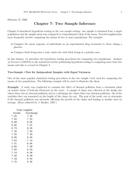
Judging from Figure 9.3.2, there was an apparent decrease in alpha-wave
frequency for persons in solitary confinement. There also appears to have been
an increase in the variability for that group. We will use the F test to determine
whether the observed difference in variability (s X2 = 0.21 versus sY2 = 0.36) is
statistically significant.
(Continued on next page)
9.3 Testing H0 : σX2 = σY2 —The F Test
473
Alpha-wave frequency (cps)
11
10
Nonconfined
Solitary
9
0
Figure 9.3.2 Alpha-wave frequencies (cps).
Let Пѓ X2 and ПѓY2 denote the true variances of alpha-wave frequencies for
nonconfined and solitary-confined prisoners, respectively. The hypotheses to be
tested are
H0 : Пѓ X2 = ПѓY2
versus
H1 : Пѓ X2 = ПѓY2
Let α = 0.05 be the level of significance. Given that
10
xi = 105.8
i=1
10
10
i=1
yi = 97.8
i=1
10
i=1
xi2 = 1121.26
yi2 = 959.70
the sample variances become
s X2 =
10(1121.26) в€’ (105.8)2
= 0.21
10(9)
and
sY2 =
10(959.70) в€’ (97.8)2
= 0.36
10(9)
Dividing the sample variances gives an observed F ratio of 1.71:
F=
sY2
0.36
= 1.71
=
2
s X 0.21
Both n and m are ten, so we would expect SY2 /S X2 to behave like an F random variable with nine and nine degrees of freedom (assuming H0 : Пѓ X2 = ПѓY2 is
true). From Table A.4 in the Appendix, we see that the values cutting off areas
of 0.025 in either tail of that distribution are 0.248 and 4.03 (see Figure 9.3.3).
Since the observed F ratio falls between the two critical values, our decision
is to fail to reject H0 —a ratio of sample variances equal to 1.71 does not rule out
(Continued on next page)
474 Chapter 9 Two-Sample Inferences
(Case Study 9.3.1 continued)
the possibility that the two true variances are equal. (In light of the Comment
preceding Theorem 9.3.1, it would now be appropriate to test H0 : Ој X = ОјY using
the two-sample t test described in Section 9.2.)
F distribution with
9 and 9 degrees
of freedom
Density
Area = 0.025
Area = 0.025
4.03
0.248
Reject H0
Reject H0
Figure 9.3.3 Distribution of SY2 /S X2 when H0 is true.
Questions
9.3.1. Case Study 9.2.3 was offered as an example of testing means when the variances are not assumed equal. Was
this a correct assumption about the variances? Test at the
0.05 level of significance.
9.3.2. Two popular forms of mortgage are the thirty-year
п¬Ѓxed-rate mortgage, where the borrower has thirty years
to repay the loan at a constant rate, and the adjustablerate mortgage (ARM), one version of which is for п¬Ѓve
years with the possibility of yearly changes in the interest rate. Since the ARM offers less certainty, its rates are
usually lower than those of п¬Ѓxed-rate mortgages. However, such vehicles should show more variability in rates.
Test this hypothesis at the 0.10 level of significance using
the following samples of mortgage offerings for a loan
of $160,000 (the borrower needs $200,000, but must pay
$40,000 up front).
$160,000 Mortgage Rates
30-Year Fixed
ARM
5.500
5.500
5.250
5.125
5.875
5.625
5.250
4.875
3.875
5.125
5.000
4.750
4.375
9.3.3. Among the standard personality inventories used
by psychologists is the thematic apperception test (TAT)
in which a subject is shown a series of pictures and is asked
to make up a story about each one. Interpreted properly,
the content of the stories can provide valuable insights
into the subject’s mental well-being. The following data
show the TAT results for 40 women, 20 of whom were
the mothers of normal children and 20 the mothers of
schizophrenic children. In each case the subject was shown
the same set of 10 pictures. The п¬Ѓgures recorded were
the numbers of stories (out of 10) that revealed a positive parent–child relationship, one where the mother was
clearly capable of interacting with her child in a flexible,
open-minded way (199).
TAT Scores
Mothers of Normal
Children
8
4
2
3
4
4
1
2
6
6
1
6
3
4
4
3
Mothers of Schizophrenic
Children
1
2
3
4
2
7
0
3
1
2
2
0
1
1
4
1
3
3
2
2
2
1
3
2
(a) Test H0 : Пѓ X2 = ПѓY2 versus H1 : Пѓ X2 = ПѓY2 , where Пѓ X2 and
ПѓY2 are the variances of the scores of mothers of normal children and scores of mothers of schizophrenic
children, respectively. Let О± = 0.05.
(b) If H0 : Пѓ X2 = ПѓY2 is accepted in part (a), test H0 : Ој X = ОјY
versus H1 : Ој X = ОјY . Set О± equal to 0.05.
9.3.4. In a study designed to investigate the effects of a
strong magnetic п¬Ѓeld on the early development of mice
9.3 Testing H0 : σX2 = σY2 —The F Test
(7), 10 cages, each containing three 30-day-old albino
female mice, were subjected for a period of 12 days to
a magnetic п¬Ѓeld having an average strength of 80 Oe/cm.
Thirty other mice, housed in 10 similar cages, were not put
in the magnetic п¬Ѓeld and served as controls. Listed in the
table are the weight gains, in grams, for each of the 20 sets
of mice.
In Magnetic Field
Not in Magnetic Field
Cage
Weight Gain (g)
Cage
Weight Gain (g)
1
2
3
4
5
6
7
8
9
10
22.8
10.2
20.8
27.0
19.2
9.0
14.2
19.8
14.5
14.8
11
12
13
14
15
16
17
18
19
20
23.5
31.0
19.5
26.2
26.5
25.2
24.5
23.8
27.8
22.0
Test whether the variances of the two sets of weight gains
are significantly different. Let α = 0.05. For the mice in the
magnetic п¬Ѓeld, s X = 5.67; for the other mice, sY = 3.18.
9.3.5. Raynaud’s syndrome is characterized by the sudden impairment of blood circulation in the fingers, a
condition that results in discoloration and heat loss. The
magnitude of the problem is evidenced in the following
data, where twenty subjects (ten “normals” and ten with
Raynaud’s syndrome) immersed their right forefingers in
water kept at 19в—¦ C. The heat output (in cal/cm2 /minute) of
the forefinger was then measured with a calorimeter (105).
Normal Subjects
Patient
W.K.
M.N.
S.A.
Z.K.
J.H.
J.G.
G.K.
A.S.
T.E.
L.F.
Heat Output
(cal/cm2 /min)
2.43
1.83
2.43
2.70
1.88
1.96
1.53
2.08
1.85
2.44
x = 2.11
s X = 0.37
Subjects with
Raynaud’s Syndrome
Patient
R.A.
R.M.
F.M.
K.A.
H.M.
S.M.
R.M.
G.E.
B.W.
N.E.
Heat Output
(cal/cm2 /min)
0.81
0.70
0.74
0.36
0.75
0.56
0.65
0.87
0.40
0.31
y = 0.62
sY = 0.20
475
Test that the heat-output variances for normal subjects and those with Raynaud’s syndrome are the
same. Use a two-sided alternative and the 0.05 level of
significance.
9.3.6. The bitter, eight-month baseball strike that ended
the 1994 season so abruptly was expected to have substantial repercussions at the box office when the 1995
season п¬Ѓnally got under way. It did. By the end of the
п¬Ѓrst week of play, American League teams were playing to 12.8% fewer fans than the year before; National
League teams fared even worse—their attendance was
down 15.1% (190). Based on the team-by-team attendance п¬Ѓgures given below, would it be appropriate to use
the pooled two-sample t test of Theorem 9.2.2 to assess
the statistical significance of the difference between those
two means?
American League
Team
Change
Baltimore
–2%
Boston
+16
California
+7
Chicago
–27
Cleveland
No home games
Detroit
–22
Kansas City
–20
Milwaukee
–30
Minnesota
–8
New York
–2
Oakland
No home games
Seattle
–3
Texas
–39
Toronto
–24
Average:
–12.8%
National League
Team
Change
Atlanta
–49%
Chicago
–4
Cincinnati
–18
Colorado
–27
Florida
–15
Houston
–16
Los Angeles
–10
Montreal
–1
New York
+34
Philadelphia
–9
Pittsburgh
–28
San Diego
–10
San Francisco
–45
St. Louis
–14
Average:
–15.1%
9.3.7. For the data in Question 9.2.8, the sample variances
for the methylmercury half-lives are 227.77 for the females
and 65.25 for the males. Does the magnitude of that difference invalidate using Theorem 9.2.2 to test H0 : Ој X = ОјY ?
Explain.
9.3.8. Crosstown busing to compensate for de facto segregation was begun on a fairly large scale in Nashville during
the 1960s. Progress was made, but critics argued that too
many racial imbalances were left unaddressed. Among
the data cited in the early 1970s are the following п¬Ѓgures,
showing the percentages of African-American students
enrolled in a random sample of eighteen public schools
(165). Nine of the schools were located in predominantly
African-American neighborhoods; the other nine, in predominantly white neighborhoods. Which version of the
two-sample t test, Theorem 9.2.2 or the Behrens–Fisher
approximation given in Theorem 9.2.3, would be more
476 Chapter 9 Two-Sample Inferences
appropriate for deciding whether the difference between
35.9% and 19.7% is statistically significant? Justify
your answer.
Schools in African-American
Neighborhoods
Schools in White
Neighborhoods
36%
28
41
32
46
39
24
32
45
Average: 35.9%
21%
14
11
30
29
6
18
25
23
Average: 19.7%
9.3.9. Show that the generalized likelihood ratio for
testing H0 : Пѓ X2 = ПѓY2 versus H1 : Пѓ X2 = ПѓY2 as described in
Theorem 9.3.1 is given by
n/2
n
О»=
L(П‰e ) (m + n)(n+m)/2
=
L( e )
n n/2 m m/2
(xi в€’ x)
ВЇ 2
i=1
n
m/2
m
(y j в€’ yВЇ )2
j=1
(xi в€’ x)
ВЇ +
m
2
i=1
(m+n)/2
(y j в€’ yВЇ )
2
j=1
9.3.10. Let X 1 , X 2 , . . . , X n and Y1 ,Y2 , . . . , Ym be independent random samples from normal distributions with
means Ој X and ОјY and standard deviations Пѓ X and ПѓY ,
respectively, where Ој X and ОјY are known. Derive the
GLRT for H0 : Пѓ X2 = ПѓY2 versus H1 : Пѓ X2 > ПѓY2 .
9.4 Binomial Data: Testing H0: pX = pY
Up to this point, the data considered in this chapter have been independent random
samples of sizes n and m drawn from two continuous distributions—in fact, from two
normal distributions. Other scenarios, of course, are quite possible. The X ’s and Y ’s
might represent continuous random variables but have density functions other than
the normal. Or they might be discrete. In this section we consider the most common
example of this latter type: situations where the two sets of data are binomial.
Applying the Generalized Likelihood Ratio Criterion
Suppose that n Bernoulli trials related to treatment X have resulted in x successes,
and that m (independent) Bernoulli trials related to treatment Y have yielded y
successes. We wish to test whether p X and pY , the true probabilities of success for
treatment X and treatment Y, are equal:
H0 : p X = pY (= p)
versus
H1 : p X = pY
Let α be the level of significance.
Following the notation used for GLRTs, the two parameter spaces here are
ω = {( p X , pY ): 0 ≤ p X = pY ≤ 1}
and
= {( p X , pY ): 0 ≤ p X ≤ 1, 0 ≤ pY ≤ 1}
Furthermore, the likelihood function can be written
y
L = p xX (1 в€’ p X )nв€’x В· pY (1 в€’ pY )mв€’y
9.4 Binomial Data: Testing H0 : pX = pY
477
Setting the derivative of ln L with respect to p(= p X = pY ) equal to 0 and solving for
p gives a not-too-surprising result—namely,
pe =
x+y
n+m
That is, the maximum likelihood estimate for p under H0 is the pooled success
proportion. Similarly, solving ∂lnL/∂ p X = 0 and ∂lnL/∂ pY = 0 gives the two original sample proportions as the unrestricted maximum likelihood estimates, for p X
and pY :
x
y
p X e = , p Ye =
n
m
Putting pe , p X e , and pYe back into L gives the generalized likelihood ratio:
x+y
О»=
n+mв€’xв€’y
(x + y)/(n + m)
1 в€’ (x + y)/(n + m)
L(П‰e )
=
nв€’x
L( e )
(x/n)x 1 в€’ (x/n)
(y/m) y 1 в€’ (y/m)
mв€’y
(9.4.1)
Equation 9.4.1 is such a difficult function to work with that it is necessary to
п¬Ѓnd an approximation to the usual generalized likelihood ratio test. There are several available. It can be shown, for example, that в€’2 ln О» for this problem has an
asymptotic П‡ 2 distribution with 1 degree of freedom (200). Thus, an approximate
two-sided, α = 0.05 test is to reject H0 if −2 ln λ ≥ 3.84.
Another approach, and the one most often used, is to appeal to the central limit
theorem and make the observation that
X
n
в€’ mY в€’ E
X
n
Var
X
n
в€’ mY
в€’ mY
has an approximate standard normal distribution. Under H0 , of course,
E
X Y
в€’
n
m
=0
and
Var
X Y
в€’
n
m
=
p(1 в€’ p) p(1 в€’ p)
+
n
m
=
(n + m) p(1 в€’ p)
nm
x+y
, its maximum likelihood estimate under П‰, we get the
If p is now replaced by n+m
statement of Theorem 9.4.1.
Theorem
9.4.1
Let x and y denote the numbers of successes observed in two independent sets of n
and m Bernoulli trials, respectively, where p X and pY are the true success probabilities
x+y
and define
associated with each set of trials. Let pe = n+m
z=
x
n
в€’ my
pe (1в€’ pe )
n
+
pe (1в€’ pe )
m
a. To test H0 : p X = pY versus H1 : p X > pY at the α level of significance, reject H0 if
z ≥ zα .
b. To test H0 : p X = pY versus H1 : p X < pY at the α level of significance, reject H0 if
z ≤ −z α .
478 Chapter 9 Two-Sample Inferences
c. To test H0 : p X = pY versus H1 : p X = pY at the α level of significance, reject H0 if z
is either (1) ≤ −z α/2 or (2) ≥ z α/2 .
Comment The utility of Theorem 9.4.1 actually extends beyond the scope we have
just described. Any continuous variable can always be dichotomized and “transformed” into a Bernoulli variable. For example, blood pressure can be recorded in
terms of “mm Hg,” a continuous variable, or simply as “normal” or “abnormal,” a
Bernoulli variable. The next two case studies illustrate these two sources of binomial
data. In the first, the measurements begin and end as Bernoulli variables; in the second, the initial measurement of “number of nightmares per month” is dichotomized
into “often” and “seldom.”
Case Study 9.4.1
Until almost the end of the nineteenth century, the mortality associated with
surgical operations—even minor ones—was extremely high. The major problem was infection. The germ theory as a model for disease transmission was still
unknown, so there was no concept of sterilization. As a result, many patients
died from postoperative complications.
The major breakthrough that was so desperately needed п¬Ѓnally came when
Joseph Lister, a British physician, began reading about some of the work done
by Louis Pasteur. In a series of classic experiments, Pasteur had succeeded
in demonstrating the role that yeasts and bacteria play in fermentation. Lister conjectured that human infections might have a similar organic origin. To
test his theory he began using carbolic acid as an operating-room disinfectant.
He performed forty amputations with the aid of carbolic acid, and thirty-four
patients survived. He also did thirty-п¬Ѓve amputations without carbolic acid, and
nineteen patients survived. While it seems clear that carbolic acid did improve
survival rates, a test of statistical significance helps to rule out a difference due
to chance (202).
Let p X be the true probability of survival with carbolic acid, and let pY
denote the true survival probability without the antiseptic. The hypotheses to
be tested are
H0 : p X = pY (= p)
versus
H1 : p X > pY
Take О± = 0.01.
If H0 is true, the pooled estimate of p would be the overall survival rate.
That is,
34 + 19 53
=
= 0.707
pe =
40 + 35 75
The sample proportions for survival with and without carbolic acid are 34/40 =
0.850 and 19/35 = 0.543, respectively. According to Theorem 9.4.1, then, the test
statistic is
0.850 в€’ 0.543
z=
= 2.92
(0.707)(0.293)
(0.707)(0.293)
+
40
35
Since z exceeds the О± = 0.01 critical value (z .01 = 2.33), we should reject the null
hypothesis and conclude that the use of carbolic acid saves lives.
9.4 Binomial Data: Testing H0 : pX = pY
479
About the Data In spite of this study and a growing body of similar evidence, the
theory of antiseptic surgery was not immediately accepted in Lister’s native England. Continental European surgeons, though, understood the value of Lister’s work
and in 1875 presented him with a humanitarian award.
Case Study 9.4.2
Over the years, numerous studies have sought to characterize the nightmare
sufferer. Out of these has emerged the stereotype of someone with high anxiety, low ego strength, feelings of inadequacy, and poorer-than-average physical
health. What is not so well known, though, is whether men fall into this pattern
with the same frequency as women. To this end, a clinical survey (77) looked at
nightmare frequencies for a sample of 160 men and 192 women. Each subject
was asked whether he (or she) experienced nightmares “often” (at least once
a month) or “seldom” (less than once a month). The percentages of men and
women saying “often” were 34.4% and 31.3%, respectively (see Table 9.4.1).
Is the difference between those two percentages statistically significant?
Table 9.4.1 Frequency of Nightmares
Nightmares often
Nightmares seldom
Totals
% often:
Men
Women
Total
55
105
160
34.4
60
132
192
31.3
115
237
Let p M and pW denote the true proportions of men having nightmares
often and women having nightmares often, respectively. The hypotheses to be
tested are
H0 : p M = pW
versus
H1 : p M = pW
Let О± = 0.05. Then В± z .025 = В± 1.96 become the two critical values. Moreover,
55 + 60
= 0.327, so
pe = 160
+ 192
0.344 в€’ 0.313
z=
(0.327)(0.673)
+ (0.327)(0.673)
160
192
= 0.62
The conclusion, then, is clear: We fail to reject the null hypothesis—these data
provide no convincing evidence that the frequency of nightmares is different for
men than for women.
About the Data The results of every statistical study are intended to be
generalized—from the subjects measured to a broader population that the sample
might reasonably be expected to represent. Obviously, then, knowing something
480 Chapter 9 Two-Sample Inferences
about the subjects is essential if a set of data is to be interpreted (and extrapolated)
properly. Table 9.4.1 is a cautionary case in point. The 352 individuals interviewed
were not the typical sort of subjects solicited for a university research project. They
were all institutionalized mental patients.
Questions
9.4.1. The phenomenon of handedness has been extensively studied in human populations. The percentages of
adults who are right-handed, left-handed, and ambidextrous are well documented. What is not so well known is
that a similar phenomenon is present in lower animals.
Dogs, for example, can be either right-pawed or leftpawed. Suppose that in a random sample of 200 beagles, it
is found that 55 are left-pawed and that in a random sample of 200 collies, 40 are left-pawed. Can we conclude that
the difference in the two sample proportions of left-pawed
dogs is statistically significant for α = 0.05?
9.4.2. In a study designed to see whether a controlled
diet could retard the process of arteriosclerosis, a total of
846 randomly chosen persons were followed over an eightyear period. Half were instructed to eat only certain foods;
the other half could eat whatever they wanted. At the end
of eight years, 66 persons in the diet group were found
to have died of either myocardial infarction or cerebral
infarction, as compared to 93 deaths of a similar nature in
the control group (203). Do the appropriate analysis. Let
О± = 0.05.
9.4.3. Water witching, the practice of using the movements of a forked twig to locate underground water (or
minerals), dates back over 400 years. Its п¬Ѓrst detailed
description appears in Agricola’s De re Metallica, published in 1556. That water witching works remains a belief
widely held among rural people in Europe and throughout the Americas. [In 1960 the number of “active” water
witches in the United States was estimated to be more
than 20,000 (193).] Reliable evidence supporting or refuting water witching is hard to п¬Ѓnd. Personal accounts of
isolated successes or failures tend to be strongly biased
by the attitude of the observer. Of all the wells dug in
Fence Lake, New Mexico, 29 “witched” wells and 32 “nonwitched” wells were sunk. Of the “witched” wells, 24
were successful. For the “nonwitched” wells, there were
27 successes. What would you conclude?
9.4.4. If flying saucers are a genuine phenomenon, it
would follow that the nature of sightings (that is, their
physical characteristics) would be similar in different parts
of the world. A prominent UFO investigator compiled a
listing of 91 sightings reported in Spain and 1117 reported
elsewhere. Among the information recorded was whether
the saucer was on the ground or hovering. His data are
summarized in the following table (87). Let p S and p N S
denote the true probabilities of “Saucer on ground” in
Spain and not in Spain, respectively. Test H0 : p S = p N S
against a two-sided H1 . Let О± = 0.01.
Saucer on ground
Saucer hovering
In Spain
Not in Spain
53
38
705
412
9.4.5. In some criminal cases, the judge and the defendant’s lawyer will enter into a plea bargain, where the
accused pleads guilty to a lesser charge. The proportion of
time this happens is called the mitigation rate. A Florida
Corrections Department study showed that Escambia
County had the state’s fourth highest rate, 61.7% (1033
out of 1675 cases). Concerned that the guilty were not getting appropriate sentences, the state attorney put in new
policies to limit the number of plea bargains. A followup study (133) showed that the mitigation rate dropped
to 52.1% (344 out of 660 cases). Is it fair to conclude that
the drop was due to the new policies, or can the decline be
written off to chance? Test at the О± = 0.01 level.
9.4.6. Suppose H0 : p X = pY is being tested against
H1 : p X = pY on the basis of two independent sets of one
hundred Bernoulli trials. If x, the number of successes
in the п¬Ѓrst set, is sixty and y, the number of successes
in the second set, is forty-eight, what P-value would be
associated with the data?
9.4.7. A total of 8605 students are enrolled full-time at
State University this semester, 4134 of whom are women.
Of the 6001 students who live on campus, 2915 are women.
Can it be argued that the difference in the proportion of
men and women living on campus is statistically significant? Carry out an appropriate analysis. Let α = 0.05.
9.4.8. The kittiwake is a seagull whose mating behavior
is basically monogamous. Normally, the birds separate for
several months after the completion of one breeding season and reunite at the beginning of the next. Whether or
not the birds actually do reunite, though, may be affected
by the success of their “relationship” the season before.
A total of 769 kittiwake pair-bonds were studied (30) over
the course of two breeding seasons; of those 769, some 609
successfully bred during the п¬Ѓrst season; the remaining 160
were unsuccessful. The following season, 175 of the previously successful pair-bonds “divorced,” as did 100 of the
160 whose prior relationship left something to be desired.
9.5 Confidence Intervals for the Two-Sample Problem
Can we conclude that the difference in the two divorce
rates (29% and 63%) is statistically significant?
Breeding in Previous Year
Number divorced
Number not divorced
Total
Percent divorced
Successful
Unsuccessful
175
434
609
29
100
60
160
63
481
9.4.9. A utility infielder for a National League club batted
.260 last season in three hundred trips to the plate. This
year he hit .250 in two hundred at-bats. The owners are
trying to cut his pay for next year on the grounds that his
output has deteriorated. The player argues, though, that
his performances the last two seasons have not been significantly different, so his salary should not be reduced.
Who is right?
9.4.10. Compute в€’2 ln О» (see Equation 9.4.1) for the
nightmare data of Case Study 9.4.2, and use it to test the
hypothesis that p X = pY . Let О± = 0.01.
9.5 Confidence Intervals for the Two-Sample Problem
Two-sample data lend themselves nicely to the hypothesis testing format because
a meaningful H0 can always be defined (which is not the case for every set of onesample data). The same inferences, though, can just as easily be phrased in terms of
confidence intervals. Simple inversions similar to the derivation of Equation 7.4.1
will yield confidence intervals for μ X − μY , σ X2 /σY2 , and p X − pY .
Theorem
9.5.1
Let x1 , x2 , . . . , xn and y1 , y2 , . . . , ym be independent random samples drawn from normal distributions with means Ој X and ОјY , respectively, and with the same standard
deviation, σ . Let s p denote the data’s pooled standard deviation. A 100(1 − α)%
confidence interval for μ X − μY is given by
xВЇ в€’ yВЇ в€’ tО±/2, n+mв€’2 В· s p
1
1
+ , xВЇ в€’ yВЇ + tО±/2, n+mв€’2 В· s p
n m
1
1
+
n m
Proof We know from Theorem 9.2.1 that
X в€’ Y в€’ (Ој X в€’ ОјY )
Sp
1
n
+ m1
has a Student t distribution with n + m в€’ 2 df. Therefore,
вЋЎ
вЋ¤
X
в€’
Y
в€’
(Ој
в€’
Ој
)
X
Y
P ⎣−tα/2, n+m−2 ≤
≤ tα/2, n+m−2 ⎦ = 1 − α
1
1
Sp n + m
(9.5.1)
Rewriting Equation 9.5.1 by isolating Ој X в€’ ОјY in the center of the inequalities gives
the endpoints stated in the theorem.
Case Study 9.5.1
Case Study 8.2.2 made the claim that X-rays penetrate the tooth enamel of men
and women differently, a fact that allows dental structure to help identify the
sex of badly decomposed bodies. In this case study, the statistical analysis for
(Continued on next page)
482 Chapter 9 Two-Sample Inferences
(Case Study 9.5.1 continued)
that assertion is provided. Moreover, the resulting confidence interval gives an
estimate of the difference in the mean enamel spectropenetration gradients for
the two sexes.
Listed in Table 9.5.1 (and Table 8.2.2) are the gradients for eight female
teeth and eight male teeth (57). These numbers are measures of the rate of
change in the amount of X-ray penetration through a 500-micron section of
tooth enamel at a wavelength of 600 nm as opposed to 400 nm.
Table 9.5.1 Enamel Spectropenetration Gradients
Male, xi
Female, yi
4.9
5.4
5.0
5.5
5.4
6.6
6.3
4.3
4.8
5.3
3.7
4.1
5.6
4.0
3.6
5.0
Let Ој X and ОјY be the population means of the spectropenetration gradients
associated with male teeth and with female teeth, respectively. Note that
8
8
xi = 43.4
xi2 = 239.32
and
i=1
i=1
from which
xВЇ =
and
s X2 =
43.4
= 5.4
8
8(239.32) в€’ (43.4)2
= 0.55
8(7)
Similarly,
8
8
yi = 36.1
i=1
yi2 = 166.95
and
i=1
so that
yВЇ =
and
sY2 =
36.1
= 4.5
8
8(166.95) в€’ (36.1)2
= 0.58
8(7)
Therefore, the pooled standard deviation is equal to 0.75:
7(0.55) + 7(0.58) в€љ
sP =
= 0.565 = 0.75
8+8в€’2
(Continued on next page)
9.5 Confidence Intervals for the Two-Sample Problem
483
We know that the ratio
X в€’ Y в€’ (Ој X в€’ ОјY )
Sp
1
8
+ 18
will be approximated by a Student t curve with 14 degrees of freedom. Since
t.025,14 = 2.1448, the 95% confidence interval for μ X − μY is given by
1 1
1 1
+ , xВЇ в€’ yВЇ + 2.1448 s p
+
8 8
8 8
в€љ
в€љ
= 5.4 в€’ 4.5 в€’ 2.1448(0.75) 0.25 , 5.4 в€’ 4.5 + 2.1448(0.75) 0.25
xВЇ в€’ yВЇ в€’ 2.1448 s p
= (0.1, 1.7)
Comment Here the 95% confidence interval does not include the value 0. This
means that had we tested
H0 : Ој X = ОјY
versus
H1 : Ој X = ОјY
at the α = 0.05 level of significance, H0 would have been rejected.
Comment For the scenario of Theorem of 9.5.1, if the variances are not equal, then
an approximate 100(1 − α)% confidence interval is given by
вЋћ
вЋ›
2
2
2
2
вЋќxВЇ в€’ yВЇ в€’ tО±/2,v s X + sY , xВЇ в€’ yВЇ + tО±/2,ОЅ s X + sY вЋ n
m
n
m
where ОЅ =
Л† n
Оё+
m
2
for ОёЛ† =
s 2X
sY2
.
( )
If the degrees or freedom exceed 100, then the form above is used, with z О±/2
replacing tО±/2,v .
Theorem
9.5.2
1 Л†2
1
(nв€’1) Оё + (mв€’1)
n 2
m
Let x1 , x2 , . . . , xn and y1 , y2 , . . . , ym be independent random samples drawn from normal distributions with standard deviations Пѓ X and ПѓY , respectively. A 100(1 в€’ О±)%
confidence interval for the variance ratio, σ X2 /σY2 , is given by
s X2
s2
F
, X2 F1в€’О±/2,mв€’1,nв€’1
2 О±/2,mв€’1,nв€’1
sY
sY
Proof Start with the fact that
SY2 /ПѓY2
S 2X /Пѓ X2
has an F distribution with m в€’ 1 and n в€’ 1 df,
and follow the strategy used in the proof of Theorem 9.5.1—that is, isolate σ X2 /σY2 in
the center of the analogous inequalities.
484 Chapter 9 Two-Sample Inferences
Case Study 9.5.2
The easiest way to measure the movement, or flow, of a glacier is with a camera. First a set of reference points is marked off at various sites near the
glacier’s edge. Then these points, along with the glacier, are photographed
from an airplane. The problem is this: How long should the time interval
be between photographs? If too short a period has elapsed, the glacier will
not have moved very far and the errors associated with the photographic
technique will be relatively large. If too long a period has elapsed, parts
of the glacier might be deformed by the surrounding terrain, an eventuality that could introduce substantial variability into the point-to-point velocity
estimates.
Two sets of flow rates for the Antarctic’s Hoseason Glacier have been calculated (115), one based on photographs taken three years apart, the other, five
years apart (see Table 9.5.2). On the basis of other considerations, it can be
assumed that the “true” flow rate was constant for the eight years in question.
Table 9.5.2 Flow Rates Estimated for the Hoseason
Glacier (Meters per Day)
Three-Year Span, xi
Five-Year Span, yi
0.73
0.76
0.75
0.77
0.73
0.75
0.74
0.72
0.74
0.74
0.72
0.72
The objective here is to assess the relative variabilities associated with the
three- and five-year time periods. One way to do this—assuming the data to be
normal—is to construct, say, a 95% confidence interval for the variance ratio.
If that interval does not contain the value 1, we infer that the two time periods
lead to flow rate estimates of significantly different precision.
From Table 9.5.2,
7
7
xi = 5.23
xi2 = 3.9089
and
i=1
i=1
so that
s X2 =
7(3.9089) в€’ (5.23)2
= 0.000224
7(6)
Similarly,
5
5
yi = 3.64
i=1
yi2 = 2.6504
and
i=1
(Continued on next page)
9.5 Confidence Intervals for the Two-Sample Problem
485
making
sY2 =
5(2.6504) в€’ (3.64)2
= 0.000120
5(4)
The two critical values come from Table A.4 in the Appendix:
F.025,4,6 = 0.109
and
F.975,4,6 = 6.23
Substituting, then, into the statement of Theorem 9.5.2 gives (0.203, 11.629) as
a 95% confidence interval for σ X2 /σY2 :
0.000224
0.000224
0.109,
6.23 = (0.203, 11.629)
0.000120
0.000120
Thus, although the three-year data have a larger sample variance than the п¬Ѓveyear data, no conclusions can be drawn about the true variances being different,
because the ratio σ X2 /σY2 = 1 is contained in the confidence interval.
Theorem
9.5.3
Let x and y denote the numbers of successes observed in two independent sets of n
and m Bernoulli trials, respectively. If p X and pY denote the true success probabilities,
an approximate 100(1 − α)% confidence interval for p X − pY is given by
вЋЎ
y
x
1 в€’ nx
1 в€’ my
n
вЋЈ x в€’ y в€’ z О±/2
+ m
,
n m
n
m
вЋ¤
y
x
в€’ + z О±/2
n m
x
n
1 в€’ nx
+
n
y
m
1 в€’ my
вЋ¦
m
Proof See Question 9.5.11.
Case Study 9.5.3
If a hospital patient’s heart stops, an emergency message, code blue, is called.
A team rushes to the bedside and attempts to revive the patient. A study (131)
suggests that patients are better off not suffering cardiac arrest after 11 p.m., the
so-called graveyard shift. The study lasted seven years and used non–emergency
room data from over п¬Ѓve hundred hospitals. During the day and early evening
hours, 58,593 cardiac arrests occurred and 11,604 patients survived to leave the
hospital. For the 11 p.m. shift, of the 28,155 heart stoppages, 4139 patients lived
to be discharged.
Let p X (estimated by 11,604/58,593 = 0.198) be the true probability of survival during the earlier hours. Let pY denote the true survival probability for the
graveyard shift (estimated by 4139/28,155 = 0.147). To construct a 95% confidence interval for p X − pY , take z α/2 = 1.96. Then Theorem 9.5.3 gives the lower
limit of the confidence interval as
0.198 в€’ 0.147 в€’ 1.96
(0.198)(0.802) (0.147)(0.853)
+
= 0.0458
58,593
28,155
(Continued on next page)
486 Chapter 9 Two-Sample Inferences
(Case Study 9.5.3 continued)
and the upper limit as
0.198 в€’ 0.147 + 1.96
(0.198)(0.802) (0.147)(0.853)
+
= 0.0562
58,593
28,155
so the 95% confidence interval is (0.0458, 0.0562).
Since p X в€’ pY = 0 is not included in the interval (which lies entirely to the
right of 0), we can conclude that survival rates are worse during the graveyard
shift.
Questions
9.5.1 In 1965 a silver shortage in the United States
prompted Congress to authorize the minting of silverless
dimes and quarters. They also recommended that the silver content of half-dollars be reduced from 90% to 40%.
Historically, fluctuations in the amount of rare metals
found in coins are not uncommon (76). The following data
may be a case in point. Listed are the silver percentages
found in samples of a Byzantine coin minted on two separate occasions during the reign of Manuel I (1143–1180).
Construct a 90% confidence interval for μ X − μY , the true
average difference in the coin’s silver content (= “early” −
“late”). What does the interval imply about the outcome
of testing H0 : Ој X = ОјY ? For these data s X = 0.54 and sY =
0.36.
Early Coinage, xi
(% Ag)
5.9
6.8
6.4
7.0
6.6
7.7
7.2
6.9
6.2
Average: 6.7
Late Coinage, yi
(% Ag)
5.3
5.6
5.5
5.1
6.2
5.8
5.8
Average: 5.6
9.5.2 Male п¬Ѓddler crabs solicit attention from the opposite sex by standing in front of their burrows and waving
their claws at the females who walk by. If a female likes
what she sees, she pays the male a brief visit in his burrow. If everything goes well and the crustacean chemistry
clicks, she will stay a little longer and mate. In what may
be a ploy to lessen the risk of spending the night alone,
some of the males build elaborate mud domes over their
burrows. Do the following data (215) suggest that a male’s
time spent waving to females is influenced by whether his
burrow has a dome? Answer the question by constructing
and interpreting a 95% confidence interval for μ X − μY .
Use the value s p = 11.2.
% of Time Spent Waving to Females
Males with Domes, xi
100.0
58.6
93.5
83.6
84.1
Males without Domes, yi
76.4
84.2
96.5
88.8
85.3
79.1
83.6
9.5.3 Construct two 99% confidence intervals for μ X − μY
using the data of Case Study 9.2.3, п¬Ѓrst assuming the
variances are equal, and then assuming they are not.
9.5.4 Carry out the details to complete the proof of
Theorem 9.5.1.
9.5.5 Suppose that X 1 , X 2 , . . . , X n and Y1 , Y2 , . . . , Ym are
independent random samples from normal distributions
with means Ој X and ОјY and known standard deviations
σ X and σY , respectively. Derive a 100(1 − α)% confidence
interval for Ој X в€’ ОјY .
9.5.6 Construct a 95% confidence interval for σ X2 /σY2
based on the data in Case Study 9.2.1. The hypothesis test
referred to tacitly assumed that the variances were equal.
Does that agree with your confidence interval? Explain.
9.5.7 One of the parameters used in evaluating myocardial function is the end diastolic volume (EDV). The following table shows EDVs recorded for eight persons considered to have normal cardiac function and for six with
constrictive pericarditis (192). Would it be correct to use
Theorem 9.2.2 to test H0 : Ој X = ОјY ? Answer the question
by constructing a 95% confidence interval for σ X2 /σY2 .
9.6 Taking a Second Look at Statistics (Choosing Samples)
Normal, xi
62
60
78
62
49
67
80
48
Constrictive Pericarditis, yi
24
56
42
74
44
28
487
9.5.10 Construct an 80% confidence interval for the
difference p M в€’ pW in the nightmare frequency data
summarized in Case Study 9.4.2.
9.5.11 If p X and pY denote the true success probabilities
associated with two sets of n and m independent Bernoulli
trials, respectively, the ratio
X
n
в€’ mY в€’ ( p X в€’ pY )
(X/n)(1в€’X/n)
n
+ (Y/m)(1в€’Y/m)
m
9.5.8 Complete the proof of Theorem 9.5.2.
9.5.9 Flonase is a nasal spray for diminishing nasal allergic
symptoms. In clinical trials for side effects, 782 sufferers
from allergic rhinitis were given a daily dose of 200 mcg of
Flonase. Of this group, 126 reported headaches. A group
of 758 subjects were given a placebo, and 111 of them
reported headaches. Find a 95% confidence interval for
the difference in proportion of headaches for the two
groups. Does the confidence interval suggest a statistically
significant difference in the frequency of headaches for
Flonase users?
Source: http://www.drugs.com/sfx/flonase-side-effects.html.
has approximately a standard normal distribution. Use
that fact to prove Theorem 9.5.3.
9.5.12 Suicide rates in the United States tend to be much
higher for men than for women, at all ages. That pattern may not extend to all professions, though. Death
certificates obtained for the 3637 members of the American Chemical Society who died over a twenty-year period
revealed that 106 of the 3522 male deaths were suicides, as
compared to 13 of the 115 female deaths (101). Construct
a 95% confidence interval for the difference in suicide
rates. What would you conclude?
9.6 Taking a Second Look at Statistics (Choosing
Samples)
Choosing sample sizes is a topic that invariably receives extensive coverage whenever applied statistics and experimental design are discussed. For good reason.
Whatever the context, the number of observations making up a data set п¬Ѓgures
prominently in the ability of those data to address any and all of the questions raised
by the experimenter. As sample sizes get larger, we know that estimators become
more precise and hypothesis tests get better at distinguishing between H0 and H1 .
Larger sample sizes, of course, are also more expensive. The trade-off between how
many observations researchers can afford to take and how many they would like to
take is a choice that has to be made early on in the design of any experiment. If the
sample sizes ultimately decided upon are too small, there is a risk that the objectives of the study will not be fully achieved—parameters may be estimated with
insufficient precision and hypothesis tests may reach incorrect conclusions.
That said, choosing sample sizes is often not as critical to the success of an experiment as choosing sample subjects. In a two-sample design, for example, how should
we decide which particular subjects to assign to treatment X and which to treatment
Y? If the subjects comprising a sample are somehow “biased” with respect to the
measurement being recorded, the integrity of the conclusions is irretrievably compromised. There are no statistical techniques for “correcting” inferences based on
measurements that were biased in some unknown way. It is also true that biases can
be very subtle, yet still have a pronounced effect on the п¬Ѓnal measurements. That
being the case, it is incumbent on researchers to take every possible precaution at
the outset to prevent inappropriate assignments of subjects to treatments.
For example, suppose for your Senior Project you plan to study whether a new
synthetic testosterone can affect the behavior of female rats. Your intention is to set
up a two-sample design where ten rats will be given weekly injections of the new
488 Chapter 9 Two-Sample Inferences
testosterone compound and another ten rats will serve as a control group, receiving
weekly injections of a placebo. At the end of eight weeks, all twenty rats will be put
in a large community cage, and the behavior of each one will be closely monitored
for signs of aggression.
Last week you placed an order for twenty female Rattus norvegicus from the
local Rats ’R Us franchise. They arrived today, all housed in one large cage. Your
plan is to remove ten of the twenty “at random,” and then put those ten in a similarly
large cage. The ten removed will be receiving the testosterone injections; the ten
remaining in the original cage will constitute the control group. The question is,
which ten should be removed?
The obvious answer—reach in and pull out ten—is very much the wrong answer!
Why? Because the samples formed in such a way might very well be biased if, for
example, you (understandably) tended to avoid grabbing the rats that looked like
they might bite. If that were the case, the ones you drew out would be biased, by
virtue of being more passive than the ones left behind. Since the measurements ultimately to be taken deal with aggression, biasing the samples in that particular way
would be a fatal flaw. Whether the total sample size was twenty or twenty thousand,
the results would be worthless.
In general, relying on our intuitive sense of the word “random” to allocate subjects to different treatments is risky, to say the least. The correct approach would
be to number the rats from 1 to 20 and then use a random number table or a computer’s random number generator to identify the ten to be removed. Figure 9.6.1
shows the Minitab syntax for choosing a random sample of ten numbers from the
integers 1 through 20. According to this particular run of the SAMPLE routine, the
ten rats to be removed for the testosterone injections are (in order) numbers 1, 5, 8,
9, 10, 14, 15, 18, 19 and 20.
Figure 9.6.1
MTB
DATA
DATA
MTB
MTB
>
>
>
>
>
set c1
1:20
end
sample 10 c1 c2
print c2
Data Display
C2
18
1
20
19
9
10
8
15
14
5
There is a moral here. Designing, carrying out, and analyzing an experiment is
an exercise that draws on a variety of scientific, computational, and statistical skills,
some of which may be quite sophisticated. No matter how well those complex issues
are attended to, though, the enterprise will fail if the simplest and most basic aspects
of the experiment—such as assigning subjects to treatments—are not carefully
scrutinized and properly done. The Devil, as the saying goes, is in the details.
Appendix 9.A.1 A Derivation of the Two-Sample t Test (A Proof of Theorem 9.2.2)
To begin, we note that both the restricted and unrestricted parameter spaces, П‰ and
, are three dimensional:
П‰ = {(Ој X , ОјY , Пѓ ): в€’в€ћ < Ој X = ОјY < в€ћ, 0 < Пѓ < в€ћ}
and
= {(Ој X , ОјY , Пѓ ): в€’в€ћ < Ој X < в€ћ, в€’в€ћ < ОјY < в€ћ, 0 < Пѓ < в€ћ}
Appendix 9.A.1 A Derivation of the Two-Sample t Test (A Proof of Theorem 9.2.2)
489
Since the X ’s and Y ’s are independent (and normal),
n
m
L(П‰) =
f X (xi )
i=1
f Y (y j )
j=1
= в€љ
n+m
1
2ПЂ Пѓ
вЋ§
вЋЁ
вЋЎ
n
1 вЋЈ
exp в€’ 2
(xi в€’ Ој)2 +
вЋ© 2Пѓ
i=1
m
j=1
вЋ¤вЋ«
вЋ¬
(yi в€’ Ој)2 вЋ¦
вЋ­
(9.A.1.1)
where μ = μ X = μY . If we take ln L(ω) and solve ∂ln L(ω)/∂μ = 0 and ∂ln
L(ω)/∂σ 2 = 0 simultaneously, the solutions will be the restricted maximum likelihood estimates:
n
ОјП‰e =
xi +
i=1
m
yj
j=1
(9.A.1.2)
n+m
and
n
ПѓП‰2e =
(xi в€’ Ојe )2 +
i=1
m
y j в€’ Ојe
2
j=1
(9.A.1.3)
n+m
Substituting Equations 9.A.1.2 and 9.A.1.3 into Equation 9.A.1.1 gives the numerator of the generalized likelihood ratio:
eв€’1
L(П‰e ) =
2ПЂ ПѓП‰2e
(n+m)/2
Similarly, the likelihood function unrestricted by the null hypothesis is
L( ) = в€љ
1
2ПЂ Пѓ
n+m
вЋ§
вЋЎ
вЋЁ 1
exp в€’ 2 вЋЈ
вЋ© 2Пѓ
n
m
(xi в€’ Ој X )2 +
i=1
j=1
вЋ¤вЋ«
вЋ¬
(y j в€’ ОјY )2 вЋ¦
вЋ­
Here, solving
∂ ln L( )
=0
∂μ X
∂ ln L( )
=0
∂μY
∂ ln L( )
=0
∂σ 2
(9.A.1.4)
490 Chapter 9 Two-Sample Inferences
gives
Ој X e = xВЇ
ОјYe = yВЇ
n
Пѓ 2e =
m
(xi в€’ x)
ВЇ 2+
i=1
(y j в€’ yВЇ )2
j=1
n+m
If these estimates are substituted into Equation 9.A.1.4, the maximum value for
L( ) simplifies to
eв€’1 /2ПЂ Пѓ 2 e
e) =
L(
(n+m)/2
It follows, then, that the generalized likelihood ratio, О», is equal to
(n+m)/2
Пѓ 2e
L(П‰e )
О»=
=
L( e )
ПѓП‰2e
or, equivalently,
n
О»2/(n+m) =
m
ВЇ 2+
(xi в€’ x)
i=1
n
2
n xВЇ + m yВЇ
n +m
xi в€’
i=1
+
j=1
m
y j в€’ yВЇ
2
yj в€’
n xВЇ + m yВЇ
n +m
j=1
2
Using the identity
n
i=1
n xВЇ + m yВЇ
xi в€’
n+m
n
2
=
m2n
(xВЇ в€’ yВЇ )2
(n + m)2
ВЇ 2+
(xi в€’ x)
i=1
we can write О»2/(n+m) as
n
О»2/(n+m) =
=
i=1
n
y j в€’ yВЇ
2
j=1
m
ВЇ 2+
(xi в€’ x)
y j в€’ yВЇ
i=1
j=1
1+
(xв€’
ВЇ yВЇ )2
2
nm
+ n+m
(xВЇ в€’ yВЇ )2
1
n
ВЇ 2+
(xi в€’x)
i=1
=
m
ВЇ 2+
(xi в€’ x)
m
j=1
( y j в€’ yВЇ )2
1
1
n+m
n+m в€’2
(xв€’
ВЇ yВЇ )
n + m в€’ 2 + s 2 [(1/n)
+ (1/m)]
2
p
where s 2p is the pooled variance:
вЋЎ
s 2p =
n
1
вЋЈ
(xi в€’ x)
ВЇ 2+
n + m в€’ 2 i=1
m
j=1
вЋ¤
2
y j в€’ yВЇ вЋ¦
Appendix 9.A.2 Minitab Applications
491
Therefore, in terms of the observed t ratio, λ2/(n+m) simplifies to
О»2/(n+m) =
n+m в€’2
n + m в€’ 2 + t2
(9.A.1.5)
At this point the proof is almost complete. The generalized likelihood ratio criterion, rejecting H0 : μ X = μY when 0 < λ ≤ λ∗ , is clearly equivalent to rejecting the
null hypothesis when 0 < λ2/(n+m) ≤ λ∗∗ . But both of these, from Equation 9.A.1.5,
are the same as rejecting H0 when t 2 is too large. Thus the decision rule in terms
of t 2 is
Reject H0 : μ X = μY in favor of H1 : μ X = μY if t 2 ≥ t ∗2
Or, phrasing this in still another way, we should reject H0 if either t ≥ t ∗ or t ≤ −t ∗ ,
where
P(в€’t в€— < T < t в€— | H0 : Ој X = ОјY is true) = 1 в€’ О±
By Theorem 9.2.1, though, T has a Student t distribution with n + m в€’ 2 df, which
makes В±t в€— = В±tО±/2,n+mв€’2 , and the theorem is proved.
Appendix 9.A.2 Minitab Applications
Minitab has a simple command—TWOSAMPLE C1 C2—for doing a two-sample
t test on a set of xi ’s and yi ’s stored in columns C1 and C2, respectively. The same
command automatically constructs a 95% confidence interval for μ X − μY .
Figure 9.A.2.1
MTB
DATA
DATA
MTB
DATA
DATA
DATA
MTB
MTB
SUBC
>
>
>
>
>
>
>
>
>
>
set c1
0.225 0.262 0.217 0.240 0.230 0.229 0.235 0.217
end
set c2
0.209 0.205 0.196 0.210 0.202 0.207 0.224 0.223
0.220 0.201
end
name c1 �X’ c2 �Y’
twosample c1 c2;
pooled.
Two-Sample T-Test and CI: X, Y
Two-sample T for X vs Y
X
Y
N
8
10
Mean
0.2319
0.20970
StDev
0.0146
0.00966
SE Mean
0.0051
0.0031
Difference = mu (X) - mu (Y)
Estimate for difference: 0.02217
95% CI for difference: (0.01005, 0.03430)
T-Test of difference = 0 (vs not =): T-Value = 3.88 P-Value = 0.001 DF = 16
Both use Pooled StDev = 0.0121
Figure 9.A.2.1 shows the syntax for analyzing the Quintus Curtius Snodgrass
data in Table 9.2.1. Notice that a subcommand is included. If we write
MTB > twosample c1 c2
492 Chapter 9 Two-Sample Inferences
Minitab will assume the two population variances are not equal, and it will perform
the approximate t test described in Theorem 9.2.3. If the intention is to assume that
Пѓ X2 = ПѓY2 (and do the t test as described in Theorem 9.2.1), the proper syntax is
MTB > twosample c1 c2;
SUBC > pooled.
As is typical, Minitab associates the test statistic with a P-value rather than
an “Accept H0 ” or “Reject H0 ” conclusion. Here, P = 0.001, which is consistent
with the decision reached in Case Study 9.2.1 to “reject H0 at the α = 0.01 level of
significance.” Figure 9.A.2.2 shows the “unpooled” analysis of these same data. The
conclusion is the same, although the P-value has almost tripled, because both the
test statistic and its degrees of freedom have decreased (recall Question 9.2.18).
Figure 9.A.2.2
MTB
DATA
DATA
MTB
DATA
DATA
MTB
MTB
>
>
>
>
>
>
>
>
set c1
0.225 0.262 0.217 0.240 0.230 0.229 0.235 0.217
end
set c2
0.209 0.205 0.196 0.210 0.202 0.207 0.224 0.223 0.220 0.201
end
name c1 �X’ c2 �Y’
twosample c1 c2
Two-Sample T-Test and CI: X, Y
Two-sample T for X vs Y
X
Y
N
8
10
Mean
0.2319
0.20970
StDev
0.0146
0.00966
SE Mean
0.0051
0.0031
Difference = mu (X) - mu (Y)
Estimate for difference: 0.02217
95% CI for difference: (0.00900, 0.03535)
T-Test of difference = 0 (vs not =): T-Value = 3.70 P-Value = 0.003 DF = 11
Testing H0 :ОјX = ОјY Using Minitab Windows
1. Enter the two samples in C1 and C2, respectively.
2. Click on STAT, then on BASIC STATISTICS, then on 2-SAMPLE t.
3. Click on SAMPLES IN DIFFERENT COLUMNS, and type C1 in
FIRST box and C2 in SECOND box.
4. Click on ASSUME EQUAL VARIANCES (if a pooled t test is
desired).
5. Click on OPTIONS.
6. Enter value for 100 (1 в€’ О±) in CONFIDENCE LEVEL box.
7. Click on NOT EQUAL; then click on whichever H1 is desired.
8. Click on OK; click on remaining OK.

Lesson 8.4: Distance Between Points

Sample Solutions of Assignment 4 for MAT3270B: 3.1,3.2,3.3

Technical Program Session Schedule – SAC 2015

Chapter 7: Two–Sample Inference - Wright State University

Housing 2015-2016 room sign up Newsletter

SAMPLE LYAPUNOV EXPONENT FOR A CLASS - Project Euclid

10. The theorem of Pythagoras - Haese Mathematics

8. The theorem of Pythagoras - Haese Mathematics

One- and Two-Sample Tests of Hypotheses

The Mathematical Expectation of Sample Variance: A General

Point Estimation: properties of estimators 1 FINITE-SAMPLE

Two-Sample Problems

link to the paper - Department of Mathematics