2001 Solutions Manual 6th Edition Feedback Control of Dynamic Systems . . Gene F. Franklin . J. David Powell . Abbas Emami-Naeini . . . . Assisted by: H.K. Aghajan H. Al-Rahmani P. Coulot P. Dankoski S. Everett R. Fuller T. Iwata V. Jones F. Safai L. Kobayashi H-T. Lee E. Thuriyasena M. Matsuoka 2002 Chapter 2 Dynamic Models Problems and Solutions for Section 2.1 1. Write the di¤erential equations for the mechanical systems shown in Fig. 2.39. For (a) and (b), state whether you think the system will eventually decay so that it has no motion at all, given that there are non-zero initial conditions for both masses, and give a reason for your answer. Figure 2.39: Mechanical systems Solution: 2003 2004 CHAPTER 2. DYNAMIC MODELS The key is to draw the Free Body Diagram (FBD) in order to keep the signs right. For (a), to identify the direction of the spring forces on the object, let x2 = 0 and …xed and increase x1 from 0. Then the k1 spring will be stretched producing its spring force to the left and the k2 spring will be compressed producing its spring force to the left also. You can use the same technique on the damper forces and the other mass. Free body diagram for Problem 2.1(a) (a) m1 x •1 m2 x •2 = = k1 x1 b1 x_ 1 k2 (x2 x1 ) k2 (x1 k3 (x2 x2 ) y) b2 x_ 2 There is friction a¤ecting the motion of both masses; therefore the system will decay to zero motion for both masses. Free body diagram for Problem 2.1(b) m1 x •1 m2 x •2 = = k1 x1 k2 (x1 x2 ) k2 (x2 x1 ) k3 x2 b1 x_ 1 Although friction only a¤ects the motion of the left mass directly, continuing motion of the right mass will excite the left mass, and that interaction will continue until all motion damps out. 2005 Figure 2.40: Mechanical system for Problem 2.2 x2 x1 . . b1(x1 - x2) k1x1 . . b1(x1 - x2) m2 m1 k2(x1 - x2) F k2(x1 - x2) Free body diagram for Problem 2.1(c) m1 x •1 m2 x •2 = k1 x1 k2 (x1 x2 ) b1 (x_ 1 x_ 2 ) = F k2 (x2 x1 ) b1 (x_ 2 x_ 1 ) 2. Write the di¤erential equations for the mechanical systems shown in Fig. 2.40. State whether you think the system will eventually decay so that it has no motion at all, given that there are non-zero initial conditions for both masses, and give a reason for your answer. Solution: The key is to draw the Free Body Diagram (FBD) in order to keep the signs right. To identify the direction of the spring forces on the left side object, let x2 = 0 and increase x1 from 0. Then the k1 spring on the left will be stretched producing its spring force to the left and the k2 spring will be compressed producing its spring force to the left also. You can use the same technique on the damper forces and the other mass. x1 . . b2(x1 - x2) k1x1 x2 . . b2(x1 - x2) m1 m2 k2(x1 - x2) Free body diagram for Problem 2.2 k1 x2 2006 CHAPTER 2. DYNAMIC MODELS Then the forces are summed on each mass, resulting in m1 x •1 m2 x •2 = k1 x1 k2 (x1 x2 ) b1 (x_ 1 x_ 2 ) = k2 (x1 x2 ) b1 (x_ 1 x_ 2 ) k1 x2 The relative motion between x1 and x2 will decay to zero due to the damper. However, the two masses will continue oscillating together without decay since there is no friction opposing that motion and no ‡exure of the end springs is all that is required to maintain the oscillation of the two masses. 3. Write the equations of motion for the double-pendulum system shown in Fig. 2.41. Assume the displacement angles of the pendulums are small enough to ensure that the spring is always horizontal. The pendulum rods are taken to be massless, of length l, and the springs are attached 3/4 of the way down. Figure 2.41: Double pendulum Solution: 2007 θ1 3 l 4 θ2 k m m 3 l sin θ1 4 3 l sin θ 2 4 De…ne coordinates If we write the moment equilibrium about the pivot point of the left pendulem from the free body diagram, M= mgl sin 1 ml2 •1 + mgl sin 3 k l (sin 4 1 + sin 1 9 2 kl cos 16 1 2 ) cos 1 (sin 3 l = ml2 •1 4 sin 1 2) =0 Similary we can write the equation of motion for the right pendulem mgl sin 2 3 + k l (sin 4 1 sin 2 ) cos 2 3 l = ml2 •2 4 As we assumed the angles are small, we can approximate using sin 1 1, and cos 2 1. Finally the linearized equations 1 ; sin 2 2 , cos 1 of motion becomes, 9 kl ( 16 9 ml•2 + mg 2 + kl ( 16 ml•1 + mg Or 1 + 1 2) = 0 2 1) = 0 2008 CHAPTER 2. DYNAMIC MODELS •1 + g l •2 + g l 9 k ( 16 m 9 k ( 2+ 16 m + 1 1 2) = 0 2 1) = 0 4. Write the equations of motion of a pendulum consisting of a thin, 4-kg stick of length l suspended from a pivot. How long should the rod be in order for the period to be exactly 2 secs? (The inertia I of a thin stick about an endpoint is 13 ml2 . Assume is small enough that sin = .) Solution: Let’s use Eq. (2.14) M =I ; l 2 O θ mg De…ne coordinates and forces Moment about point O. MO = mg = 1 2• ml 3 l sin = IO • 2 • + 3g sin = 0 2l 2009 As we assumed is small, • + 3g = 0 2l The frequency only depends on the length of the rod !2 = 3g 2l s T = 2 =2 ! 2l =2 3g l = 3g = 1:49 m 2 2 <Notes> q 2l (a) Compare the formula for the period, T = 2 3g with the well known formula for the period of a point mass hanging with a string with q l length l. T = 2 g. (b) Important! In general, Eq. (2.14) is valid only when the reference point for the moment and the moment of inertia is the mass center of the body. However, we also can use the formular with a reference point other than mass center when the point of reference is …xed or not accelerating, as was the case here for point O. 5. For the car suspension discussed in Example 2.2, plot the position of the car and the wheel after the car hits a “unit bump” (i.e., r is a unit step) using MATLAB. Assume that m1 = 10 kg, m2 = 350 kg, kw = 500; 000 N=m, ks = 10; 000 N=m. Find the value of b that you would prefer if you were a passenger in the car. Solution: The transfer function of the suspension was given in the example in Eq. (2.12) to be: (a) Y (s) = 4 R(s) s + ( mb1 + b 3 m2 )s + kw b m1 m2 (s ks ks (m +m 1 2 + + ks b ) kw 2 m1 )s + ( mk1wmb 2 )s + kw k s m1 m2 : This transfer function can be put directly into Matlab along with the numerical values as shown below. Note that b is not the damping 2010 CHAPTER 2. DYNAMIC MODELS ratio, but damping. We need to …nd the proper order of magnitude for b, which can be done by trial and error. What passengers feel is the position of the car. Some general requirements for the smooth ride will be, slow response with small overshoot and oscillation. From the …gures, b 3000 would be acceptable. There is too much overshoot for lower values, and the system gets too fast (and harsh) for larger values. % Problem 2.5 clear all, close all m1 = 10; m2 = 350; kw = 500000; ks = 10000; B = [ 1000 2000 3000 4000 ]; t = 0:0.01:2; for i = 1:4 b = B(i); num = kw*b/(m1*m2)*[1 ks/b]; den =[1 (b/m1+b/m2) (ks/m1+ks/m2+kw/m1) (kw*b/(m1*m2) kw*ks/(m1*m2)]; sys=tf(num,den); y = step( sys, t ); subplot(2,2,i); plot( t, y(:,1), ’:’, t, y(:,2), ’-’); legend(’Wheel’,’Car’); ttl = sprintf(’Response with b = %4.1f ’,b ); title(ttl); end 6. Write the equations of motion for a body of mass M suspended from a …xed point by a spring with a constant k. Carefully de…ne where the body’s displacement is zero. Solution: Some care needs to be taken when the spring is suspended vertically in the presence of the gravity. We de…ne x = 0 to be when the spring is unstretched with no mass attached as in (a). The static situation in (b) results from a balance between the gravity force and the spring. 2011 From the free body diagram in (b), the dynamic equation results m• x= kx mg: We can manipulate the equation m• x= so if we replace x using y = x + k x+ m g ; k m k g, m• y = ky m• y + ky = 0 The equilibrium value of x including the e¤ect of gravity is at x = m kg and y represents the motion of the mass about that equilibrium point. An alternate solution method, which is applicable for any problem involving vertical spring motion, is to de…ne the motion to be with respect to the static equilibrium point of the springs including the e¤ect of gravity, and then to proceed as if no gravity was present. In this problem, we would de…ne y to be the motion with respect to the equilibrium point, then the FBD in (c) would result directly in m• y= ky: 7. Automobile manufacturers are contemplating building active suspension systems. The simplest change is to make shock absorbers with a changeable damping, b(u1 ): It is also possible to make a device to be placed in parallel with the springs that has the ability to supply an equal force, u2; in opposite directions on the wheel axle and the car body. 2012 CHAPTER 2. DYNAMIC MODELS (a) Modify the equations of motion in Example 2.2 to include such control inputs. (b) Is the resulting system linear? (c) Is it possible to use the forcer, u2; to completely replace the springs and shock absorber? Is this a good idea? Solution: (a) The FBD shows the addition of the variable force, u2 ; and shows b as in the FBD of Fig. 2.5, however, here b is a function of the control variable, u1 : The forces below are drawn in the direction that would result from a positive displacement of x. Free body diagram m1 x • = b (u1 ) (y_ x) _ + ks (y x) kw (x m2 y• = ks (y x) b (u1 ) (y_ x) _ + u2 r) u2 (b) The system is linear with respect to u2 because it is additive. But b is not constant so the system is non-linear with respect to u1 because the control essentially multiplies a state element. So if we add controllable damping, the system becomes non-linear. (c) It is technically possible. However, it would take very high forces and thus a lot of power and is therefore not done. It is a much better solution to modulate the damping coe¢ cient by changing ori…ce sizes in the shock absorber and/or by changing the spring forces by increasing or decreasing the pressure in air springs. These features are now available on some cars... where the driver chooses between a soft or sti¤ ride. 8. Modify the equation of motion for the cruise control in Example 2.1, Eq(2.4), so that it has a control law; that is, let u = K(vr v); where vr K = = reference speed constant: 2013 This is a �proportional’control law where the di¤erence between vr and the actual speed is used as a signal to speed the engine up or slow it down. Put the equations in the standard state-variable form with vr as the input and v as the state. Assume that m = 1000 kg and b = 50 N s= m; and …nd the response for a unit step in vr using MATLAB. Using trial and error, …nd a value of K that you think would result in a control system in which the actual speed converges as quickly as possible to the reference speed with no objectional behavior. Solution: 1 b v= u m m v_ + substitute in u = K (vr v) v_ + b 1 K v= u= (vr m m m v) Rearranging, yields the closed-loop system equations, v_ + b K K v + v = vr m m m A block diagram of the scheme is shown below where the car dynamics are depicted by its transfer function from Eq. 2.7. vr + Σ − 1 m b s+ m u K Block diagram The transfer function of the closed-loop system is, V (s) Vr (s) = so that the inputs for Matlab are s+ K m b K m + m v 2014 CHAPTER 2. DYNAMIC MODELS num = den = K m [1 b K + ] m m For K = 100; 500; 1000; 5000 We have, Step Response From: U(1) 1 0.9 0.8 K=500 K=1000 0.6 To: Y(1) Amplitude 0.7 K=5000 0.5 K=100 0.4 0.3 0.2 0.1 0 0 5 10 15 20 25 30 35 40 Time (sec.) Time responses We can see that the larger the K is, the better the performance, with no objectionable behaviour for any of the cases. The fact that increasing K also results in the need for higher acceleration is less obvious from the plot but it will limit how fast K can be in the real situation because the engine has only so much poop. Note also that the error with this scheme gets quite large with the lower values of K. You will …nd out how to eliminate this error in chapter 4 using integral control, which is contained in all cruise control systems in use today. For this problem, a reasonable compromise between speed of response and steady state errors would be K = 1000; where it responds is 5 seconds and the steady state error is 5%. 2015 % Problem 2.8 clear all, close all % data m = 1000; b = 50; k = [ 100 500 1000 5000 ]; % Overlay the step response hold on for i=1:length(k) K=k(i); num =K/m; den = [1 b/m+K/m]; step( num, den); end 9. In many mechanical positioning systems there is ‡exibility between one part of the system and another. An example is shown in Figure 2.6 where there is ‡exibility of the solar panels. Figure 2.42 depicts such a situation, where a force u is applied to the mass M and another mass m is connected to it. The coupling between the objects is often modeled by a spring constant k with a damping coe¢ cient b, although the actual situation is usually much more complicated than this. (a) Write the equations of motion governing this system. (b) Find the transfer function between the control input, u; and the output, y: Figure 2.42: Schematic of a system with ‡exibility Solution: (a) The FBD for the system is 2016 CHAPTER 2. DYNAMIC MODELS Free body diagrams which results in the equations m• x = k (x y) b (x_ y) _ M y• = u + k (x y) + b (x_ y) _ or k b x + x_ m m k b x x_ + y• + M M x •+ k y m k y+ M b y_ m b y_ M = 0 = 1 u M (b) If we make Laplace Transform of the equations of motion s2 X + k X M k b X + sX m m b sX + s2 Y + M k Y m k Y + M b sY m b sY M = 0 = 1 U M = 0 U In matrix form, ms2 + bs + k (bs + k) (bs + k) M s2 + bs + k X Y From Cramer’s Rule, ms2 + bs + k 0 (bs + k) U 2 ms + bs + k (bs + k) (bs + k) M s2 + bs + k det Y = det = Finally, ms2 + bs + k (ms2 + bs + k) (M s2 + bs + k) 2U (bs + k) 2017 Y U = = ms2 + bs + k 2 (ms2 + bs + k) (M s2 + bs + k) (bs + k) ms2 + bs + k mM s4 + (m + M )bs3 + (M + m)ks2 2018 CHAPTER 2. DYNAMIC MODELS Problems and Solutions for Section 2.2 10. A …rst step toward a realistic model of an op amp is given by the equations below and shown in Fig. 2.43. 107 [V+ s+1 = i =0 Vout = i+ V ] Figure 2.43: Circuit for Problem 10. Find the transfer function of the simple ampli…cation circuit shown using this model. Solution: As i = 0, (a) Vin V Rin V = Vout = = = = V Vout Rf Rf Rin Vin + Vout Rin + Rf Rin + Rf 107 [V+ V ] s+1 107 Rf V+ Vin s+1 Rin + Rf 107 s+1 Rin Vout Rin + Rf Rf Rin Vin + Vout Rin + Rf Rin + Rf 2019 Figure 2.44: Circuit for Problem 11. R f 107 Rin +R Vout f = in Vin s + 1 + 107 RinR+R f 11. Show that the op amp connection shown in Fig. 2.44 results in Vo = Vin if the op amp is ideal. Give the transfer function if the op amp has the non-ideal transfer function of Problem 2.10. Solution: Ideal case: Vin V+ V = V+ = V = Vout Non-ideal case: Vin = V+ ; V = Vout but, V+ 6= V instead, Vout = = 107 [V+ s+1 107 [Vin s+1 V ] Vout ] 2020 CHAPTER 2. DYNAMIC MODELS so, 107 107 Vout 107 = s+1107 = = Vin s + 1 + 107 s + 107 1 + s+1 12. Show that, with the non-ideal transfer function of Problem 2.10, the op amp connection shown in Fig. 2.45 is unstabl e. Figure 2.45: Circuit for Problem 12. Solution: Vin = V ; V+ = Vout Vout 107 [V+ V ] s+1 107 [Vout Vin ] s+1 = = Vout = Vin 107 s+1 107 s+1 1 = 107 107 = s 1 + 107 s 107 The transfer function has a denominator with s 107 ; and the minus sign means the exponential time function is increasing, which means that it has an unstable root. 13. A common connection for a motor power ampli…er is shown in Fig. 2.46. The idea is to have the motor current follow the input voltage and the connection is called a current ampli…er. Assume that the sense resistor, Rs is very small compared with the feedback resistor, R and …nd the transfer function from Vin to Ia : Also show the transfer function when Rf = 1: 2021 Solution: At node A, Vin 0 Vout 0 VB 0 + + =0 Rin Rf R At node B, with Rs Ia + (93) R 0 VB 0 VB + R Rs = VB = VB 0 (94) RRs Ia R + Rs Rs Ia The dynamics of the motor is modeled with negligible inductance as Jm •m + b _ m Jm s + b = Kt Ia = Kt Ia (95) At the output, from Eq. 94. Eq. 95 and the motor equation Va = Ia Ra + Ke s Vo = Ia Rs + Va = Ia Rs + Ia Ra + Ke Kt Ia Jm s + b Substituting this into Eq.93 Vin Ia Rs 1 Kt Ia + =0 + Ia Rs + Ia Ra + Ke Rin Rf Jm s + b R This expression shows that, in the steady state when s ! 0; the current is proportional to the input voltage. If fact, the current ampli…er normally has no feedback from the output voltage, in which case Rf ! 1 and we have simply Ia = Vin R Rin Rs 14. An op amp connection with feedback to both the negative and the positive terminals is shown in Fig 2.47. If the op amp has the non-ideal transfer function given in Problem 10, give the maximum value possible for the r positive feedback ratio, P = in terms of the negative feedback r+R Rin ratio,N = for the circuit to remain stable. Rin + Rf Solution: 2022 CHAPTER 2. DYNAMIC MODELS Figure 2.46: Op Amp circuit for Problem 14. Vin V Vout V + Rin Rf Vout V+ 0 V+ + R r V 0 = 0 Rf Rin Vin + Vout Rin + Rf Rin + Rf = (1 N ) Vin + N Vout r Vout = P Vout = r+R = V+ Vout = = = Vout Vin 107 [V+ V ] s+1 107 [P Vout (1 s+1 = = = N ) Vin N Vout ] 107 (1 N ) s+1 107 107 P N 1 s+1 s+1 107 (1 N ) 107 P 107 N (s + 1) 107 (1 N ) s + 1 107 P + 107 N 2023 0 < 1 107 P + 107 N P < N + 10 7 15. Write the dynamic equations and …nd the transfer functions for the circuits shown in Fig. 2.48. (a) passive lead circuit (b) active lead circuit (c) active lag circuit. (d) passive notch circuit Solution: (a) Passive lead circuit With the node at y+, summing currents into that node, we get Vu Vy R1 +C d (Vu dt Vy ) Vy =0 R2 (96) rearranging a bit, C V_ y + 1 1 + R1 R2 1 Vy = C V_ u + Vu R1 and, taking the Laplace Transform, we get Cs + R11 Vy (s) = Vu (s) Cs + R11 + R12 (b) Active lead circuit Rf V R1 R2 Vin Vout C Active lead circuit with node marked Vin V 0 V d + + C (0 R2 R1 dt V)=0 (97) 2024 CHAPTER 2. DYNAMIC MODELS 0 Vout Vin V = R2 Rf (98) We need to eliminate V . From Eq. 98, V = Vin + R2 Vout Rf Substitute V ’s in Eq. 97. 1 R2 Vin R2 Vout Rf Vin 1 Vin + C V_ in = R1 1 R1 1 Rf Vin + 1+ R2 Vout Rf R2 R1 R2 _ C V_ in + Vout Rf Vout + R2 C V_ out Laplace Transform Vout Vin = Cs + 1 Rf 1 R1 R2 Cs + 1 + R2 R1 1 = s + R1 C Rf R2 s + R11C + R21C We can see that the pole is at the left side of the zero, which means a lead compensator. (c) active lag circuit V R2 R1 C Rin Vin Vout Active lag circuit with node marked Vin 0 0 V V Vout d = = + C (V Rin R2 R1 dt R2 V = Vin Rin Vout ) =0 2025 Vin Rin = 1 Rin R2 Rin Vin = 1 R1 1+ R2 R1 Vout R1 R2 Vin Rin Vin + +C d dt Vout R2 Vin Vout Rin R2 _ +C Vin V_ out Rin 1 R2 C V_ in = Rin 1 Vout R1 C V_ out R Vout Vin R1 R2 Cs + 1 + R21 Rin R1 Cs + 1 1 1 R2 s + R2 C + R1 C = = Rin s+ 1 R1 C We can see that the pole is at the right side of the zero, which means a lag compensator. (d) notch circuit V1 C C V2 + + R R R/2 Vin Vout 2C − − Passive notch …lter with nodes marked C d 0 V1 d (Vin V1 ) + + C (Vout V1 ) = 0 dt R=2 dt Vin V2 d Vout V2 + 2C (0 V2 ) + = 0 R dt R V2 Vout d = 0 C (V1 Vout ) + dt R We need to eliminat V1 ; V2 from three equations and …nd the relation between Vin and Vout V1 = V2 = Cs 2 Cs + 1 R 1 R 2 Cs + 1 R (Vin + Vout ) (Vin + Vout ) 2026 CHAPTER 2. DYNAMIC MODELS CsV1 = Cs = 1 Vout R 1 1 R (Vin + Vout ) + R 2 Cs + CsVout + Cs 2 Cs + 1 R 1 V2 R 1 R (Vin + Vout ) Cs + 0 C 2 s2 + R12 Vin 2 Cs + R1 = " C 2 s2 + R12 2 Cs + R1 1 Cs + R # Vout C 2 s2 + R12 Vout Vin 1 2(Cs+ R ) = Cs + = 2 Cs + = = C 2 s2 + R12 1 R 1 2(Cs+ R ) C 2 s2 + 1 R2 1 2 R C 2 s2 + 1 R2 1 R2 C 2 1 C 2 s2 + 4 Cs R + R2 s2 + R21C 2 4 s2 + RC s + R21C 2 C 2 s2 + 16. The very ‡exible circuit shown in Fig. 2.49 is called a biquad because its transfer function can be made to be the ratio of two second-order or quadratic polynomials. By selecting di¤erent values for Ra ; Rb ; Rc ; and Rd the circuit can realise a low-pass, band-pass, high-pass, or band-reject (notch) …lter. (a) Show that if Ra = R; and Rb = Rc = Rd = 1; the transfer function from Vin to Vout can be written as the low-pass …lter Vout A = 2 Vin s s +2 +1 ! 2n !n where A = !n = = R R1 1 RC R 2R2 (99) 1 R Vout 2027 Figure 2.47: Op-amp biquad (b) Using the MATLAB comand step compute and plot on the same graph the step responses for the biquad of Fig. 2.43 for A = 1; ! n = 1; and = 0:1; 0:5; and 1:0: Solution: Before going in to the speci…c problem, let’s …nd the general form of the transfer function for the circuit. Vin V3 + R1 R V1 R V3 V3 V2 V1 Vin + + + Ra Rb Rc Rd V1 + C V_ 1 R2 = = C V_ 2 = V2 Vout R = There are a couple of methods to …nd the transfer function from Vin to Vout with set of equations but for this problem, we will directly solve for the values we want along with the Laplace Transform. From the …rst three equations, slove for V1; V2 . V3 Vin + R1 R V1 R V3 1 + Cs V1 R2 = = CsV2 = V2 2028 CHAPTER 2. DYNAMIC MODELS 1 1 + Cs V1 V2 R2 R 1 V1 + CsV2 R 1 R2 V1 V2 1 R + Cs 1 R 1 = 1 R2 + Cs Cs + C 2 s2 + 0 1 R1 Vin = 0 Cs 1 = = V1 V2 Cs 1 Vin R1 = C R2 s + 1 R2 1 R 1 R2 1 R2 1 R 1 R1 Vin + Cs 0 C R1 sVin 1 RR1 Vin Plug in V1 , V2 and V3 to the fourth equation. = V3 V2 V1 Vin + + + Ra Rb Rc Rd 1 1 1 1 + V2 + V1 + Vin Ra Rb Rc Rd = C 1 1 1 RR1 R1 s V + Vin + Vin in 1 1 C C 2 2 2 2 Rc C s + R s + R 2 Rd C s + R2 s + R2 2 # C 1 1 1 1 RR1 R1 s + + Vin Rb C 2 s2 + RC s + R12 Rc C 2 s2 + RC s + R12 Rd 2 2 1 1 + Ra Rb = " 1 + Ra Vout R = Finally, Vout Vin = R " = R = R C2 1 1 + Ra Rb 1 Ra + 1 Rb 1 RR1 C 2 s2 + RC2 s 1 RR1 1 C Rc R1 s C 2 s2 + C2 2 Rd s + 1 C Rd R2 1 C Rc R1 s2 + + 1 R2 1 Rd + C R2 s + s+ 1 R2 C s + C 1 R1 s + Rc C 2 s2 + RC s + 2 C 2 s2 + C R2 s + 1 R2 1 RR1 + 1 1 Rd R2 1 R2 1 Rb 1 (RC)2 1 Ra 1 R2 1 + Rd # 2029 (a) If Ra = R; and Rb = Rc = Rd = 1; Vout Vin C2 2 Rd s = R C2 = R C 2 s2 + = + 1 C Rd R2 1 C Rc R1 s2 + 1 1 R RR1 1 1 R2 C s + (RC)2 = s+ 1 R2 C s s2 + 1 Rb 1 Ra 1 RR1 + 1 1 Rd R2 1 (RC)2 1 RR1 C 2 1 1 R2 C s + (RC)2 + R R1 2 (RC) s2 + R2 C R2 s +1 So, R R1 2 !n = = = A (RC) = 2 = !n 1 ! 2n R2 C R2 1 RC ! n R2 C 1 R2 C R = = 2 R2 2RC R2 2R2 (b) Step response using MatLab % Problem 2.16 A = 1; wn = 1; z = [ 0.1 0.5 1.0 ]; hold on for i = 1:3 num = [ A ]; den = [ 1/wn^2 2*z(i)/wn 1 ] step( num, den ) end hold o¤ 17. Find the equations and transfer function for the biquad circuit of Fig. 2.49 if Ra = R; Rd = R1 and Rb = Rc = 1: Solution: 2030 CHAPTER 2. DYNAMIC MODELS Vout Vin C2 2 Rd s + 1 C Rd R2 1 C Rc R1 = R C2 = R C2 = s2 + R21C s R 1 R1 s2 + R21C s + (RC) 2 s2 + C2 2 R1 s + 1 C R1 R2 s2 + 1 R2 C s 1 R s+ 1 R2 C s s+ + + 1 RR1 1 (RC)2 1 Rb 1 Ra 1 (RC)2 + 1 1 R1 R2 1 RR1 + 1 1 Rd R2 2031 Problems and Solutions for Section 2.3 18. The torque constant of a motor is the ratio of torque to current and is often given in ounce-inches per ampere. (ounce-inches have dimension force-distance where an ounce is 1=16 of a pound.) The electric constant of a motor is the ratio of back emf to speed and is often given in volts per 1000 rpm. In consistent units the two constants are the same for a given motor. (a) Show that the units ounce-inches per ampere are proportional to volts per 1000 rpm by reducing both to MKS (SI) units. (b) A certain motor has a back emf of 25 V at 1000 rpm. What is its torque constant in ounce-inches per ampere? (c) What is the torque constant of the motor of part (b) in newton-meters per ampere? Solution: Before going into the problem, let’s review the units. Some remarks on non SI units. – Ounce 1oz = 2:835 10 2 kg Originally ounce is a unit of mass, but like pounds, it is commonly used as a unit of force. If we translate it as force, 1oz(f) = 2:835 2 10 kgf = 2:835 10 2 2 m 9:81 N = 0:2778 N – Inch 1 in = 2:540 10 – RPM (Revolution per Minute) 1 RPM = 2 rad = rad/ s 60 s 30 Relation between SI units – Voltage and Current V olts Current(amps) V olts = P ower = Energy(joules)= sec Joules= sec N ewton meters= sec = = amps amps 2032 CHAPTER 2. DYNAMIC MODELS (a) Relation between torque constant and electric constant. Torque constant: 1 ounce 1 inch 0:2778 N = 1 Ampere 2:540 1A 10 2 m = 7:056 10 3 N m= A Electric constant: 1V 1 J=(A sec) = = 9:549 1000 RPM 1000 30 rad/ s 10 3 N m= A So, 1 oz in= A = = 7:056 10 3 V=1000 RPM 9:549 10 3 (0:739) V=1000 RPM (b) 25 V=1000 RPM = 25 1 oz in= A = 33:872 oz in= A 0:739 (c) 25 V=1000 RPM = 25 9:549 10 3 N m= A = 0:239 N m= A 19. The electromechanical system shown in Fig. 2.50 represents a simpli…ed model of a capacitor microphone. The system consists in part of a parallel plate capacitor connected into an electric circuit. Capacitor plate a is rigidly fastened to the microphone frame. Sound waves pass through the mouthpiece and exert a force fs (t) on plate b, which has mass M and is connected to the frame by a set of springs and dampers. The capacitance C is a function of the distance x between the plates, as follows: C(x) = "A ; x where " = dielectric constant of the material between the plates; A = surface area of the plates: The charge q and the voltage e across the plates are related by q = C(x)e: The electric …eld in turn produces the following force fe on the movable plate that opposes its motion: fe = q2 2"A 2033 (a) Write di¤erential equations that describe the operation of this system. (It is acceptable to leave in nonlinear form.) (b) Can one get a linear model? (c) What is the output of the system? Figure 2.48: Simpli…ed model for capacitor microphone Solution: (a) The free body diagram of the capacitor plate b − Kx − Bx& M − sgn(x& )f e f s (t ) x Free body diagram So the equation of motion for the plate is Mx • + B x_ + Kx + fe sgn (x) _ = fs (t) : The equation of motion for the circuit is d i+e dt where e is the voltage across the capacitor, Z 1 e= i(t)dt C v = iR + L 2034 CHAPTER 2. DYNAMIC MODELS and where C = "A=x; a variable. Because i = can rewrite the circuit equation as v = Rq_ + L• q+ d dt q and e = q=C; we qx "A In summary, we have these two, couptled, non-linear di¤erential equation. q2 2"A qx Rq_ + L• q+ "A Mx • + bx_ + kx + sgn (x) _ = fs (t) = v (b) The sgn function, q 2 , and qx; terms make it impossible to determine a useful linearized version. (c) The signal representing the voice input is the current, i, or q: _ 20. A very typical problem of electromechanical position control is an electric motor driving a load that has one dominant vibration mode. The problem arises in computer-disk-head control, reel-to-reel tape drives, and many other applications. A schematic diagram is sketched in Fig. 2.51. The motor has an electrical constant Ke , a torque constant Kt , an armature inductance La , and a resistance Ra . The rotor has an inertia J1 and a viscous friction B. The load has an inertia J2 . The two inertias are connected by a shaft with a spring constant k and an equivalent viscous damping b. Write the equations of motion. Figure 2.49: Motor with a ‡exible load (a) Solution: (a) Rotor: J1 •1 = B _1 b _1 _2 k( 1 2) + Tm 2035 Load: J2 •2 = b _2 _1 k( 2 1) Circuit: va Ke _ 1 = La d ia + Ra ia dt Relation between the output torque and the armature current: Tm = Kt ia 2036 CHAPTER 2. DYNAMIC MODELS Problems and Solutions for Section 2.4 21. A precision-table leveling scheme shown in Fig. 2.52 relies on thermal expansion of actuators under two corners to level the table by raising or lowering their respective corners. The parameters are: Tact = actuator temperature; Tamb = ambient air temperature; Rf = heat ow coe cient between the actuator and the air; C = thermal capacity of the actuator; R = resistance of the heater: Assume that (1) the actuator acts as a pure electric resistance, (2) the heat ‡ow into the actuator is proportional to the electric power input, and (3) the motion d is proportional to the di¤erence between Tact and Tamb due to thermal expansion. Find the di¤erential equations relating the height of the actuator d versus the applied voltage vi . Figure 2.50: (a) Precision table kept level by actuators; (b) side view of one actuator Solution: Electric power in is proportional to the heat ‡ow in 2 v Q_ in = Kq i R and the heat ‡ow out is from heat transfer to the ambient air 1 Q_ out = (Tact Tamb ) : Rf 2037 The temperature is governed by the di¤erence in heat ‡ows T_act = = 1 _ Qin Q_ out C 1 v2 1 Kq i (Tact C R Rf Tamb ) and the actuator displacement is d = K (Tact Tamb ) : where Tamb is a given function of time, most likely a constant for a table inside a room. The system input is vi and the system output is d: 22. An air conditioner supplies cold air at the same temperature to each room on the fourth ‡oor of the high-rise building shown in Fig. 2.53(a). The ‡oor plan is shown in Fig. 2.53(b). The cold air ‡ow produces an equal amount of heat ‡ow q out of each room. Write a set of di¤erential equations governing the temperature in each room, where To = temperature outside the building; Ro = resistance to heat ow through the outer walls; Ri = resistance to heat ow through the inner walls: Assume that (1) all rooms are perfect squares, (2) there is no heat ‡ow through the ‡oors or ceilings, and (3) the temperature in each room is uniform throughout the room. Take advantage of symmetry to reduce the number of di¤erential equations to three. Solution: We can classify 9 rooms to 3 types by the number of outer walls they have. Type 1 Type 2 Type 1 Type 2 Type 3 Type 2 Type 1 Type 2 Type 1 We can expect the hotest rooms on the outside and the corners hotest of all, but solving the equations would con…rm this intuitive result. That is, To > T1 > T2 > T3 and, with a same cold air ‡ow into every room, the ones with some sun load will be hotest. Let’s rede…nce the resistances Ro = resistance to heat ow through one unit of outer wall Ri = resistance to heat ow through one unit of inner wall 2038 CHAPTER 2. DYNAMIC MODELS Figure 2.51: Building air conditioning: (a) high-rise building, (b) ‡oor plan of the fourth ‡oor Room type 1: T_1 = = qout = qin = 2 (T1 Ri 2 (To Ro 1 (qin qout ) C 1 2 (To T1 ) C Ro T2 ) + q T1 ) 2 (T1 Ri T2 ) q Room type 2: 1 T_2 = C qin = qout = 1 (To Ro 1 (To Ro 1 (T2 Ri T2 ) + T2 ) + 2 (T1 Ri T2 ) T3 ) + q 2 (T1 Ri T2 ) 1 (T2 Ri T3 ) q 2039 Room type 3: qout 4 (T2 Ri = q 1 T_3 = C 4 (T2 Ri qin = T3 ) T3 ) q 23. For the two-tank ‡uid-‡ow system shown in Fig. 2.54, …nd the di¤erential equations relating the ‡ow into the …rst tank to the ‡ow out of the second tank. Figure 2.52: Two-tank ‡uid-‡ow system for Problem 23 Solution: This is a variation on the problem solved in Example 2.18 and the de…nitions of terms is taken from that. From the relation between the height of the water and mass ‡ow rate, the continuity equations are m _1 m _2 = = A1 h_ 1 = win w A2 h_ 2 = w wout Also from the relation between the pressure and outgoing mass ‡ow rate, w = wout = 1 1 ( gh1 ) 2 R1 1 1 ( gh2 ) 2 R2 2040 CHAPTER 2. DYNAMIC MODELS Finally, h_ 1 = h_ 2 = 1 1 1 ( gh1 ) 2 + win A1 R1 A1 1 1 1 1 ( gh1 ) 2 ( gh2 ) 2 : A2 R1 A2 R2 24. A laboratory experiment in the ‡ow of water through two tanks is sketched in Fig. 2.55. Assume that Eq. (2.74) describes ‡ow through the equal-sized holes at points A, B, or C. (a) With holes at A and C but none at B, write the equations of motion for this system in terms of h1 and h2 . Assume that h3 = 20 cm, h1 > 20 cm; and h2 < 20 cm. When h2 = 10 cm, the out‡ow is 200 g/min. (b) At h1 = 30 cm and h2 = 10 cm, compute a linearized model and the transfer function from pump ‡ow (in cubic centimeters per minute) to h2 . (c) Repeat parts (a) and (b) assuming hole A is closed and hole B is open. Figure 2.53: Two-tank ‡uid-‡ow system for Problem 24 Solution: 2041 (a) Following the solution of Example 2.18, and assuming the area of both tanks is A; the values given for the heights ensure that the water will ‡ow according to 1 1 WA = [ g (h1 h3 )] 2 R 1 1 WC = [ gh2 ] 2 R WA WC = Ah_ 2 Win WA = Ah_ 1 From the out‡ow information given, we can compute the ori…ce resistance, R; noting that for water, = 1 gram/cc and g = 981 cm/sec2 ' 1000 cm/sec2 : 1p 1p WC = 200 g= mn = gh2 = g 10 cm R p R p 1 g= cm3 1000 cm= s2 10 cm g 10 cm R = = 200 g= mn 200 g=60 s s 1 1 g cm2 s2 100 = 60 = 30 g 2 cm 2 3 2 2 200 cm s g (b) The nonlinear equations from above are h_ 1 = h_ 2 = 1 1 p g (h1 h3 ) + Win AR A 1 p 1 p g (h1 h3 ) gh2 AR AR The square root functions need to be linearized about the nominal heights. In general the square root function can be linearized as below p x0 + x = = s p x0 1 + x x0 x0 1 + 1 x 2 x0 So let’s assume that h1 = h10 + h1 and h2 = h20 + h2 where h10 = 30 cm, h20 = 10 cm, and h3 = 20 cm. And for round numbers, let’s assume the area of each tank A = 100 cm2 : The equations above then reduce to p 1 1 h_ 1 = (1)(1000) (30 + h1 20) + Win (1)(100)(30) (1)(100) p p 1 1 h_ 2 = (1)(1000) (30 + h1 20) (1)(1000)(10 + h2 ) (1)(100)(30) (1)(100)(30) 2042 CHAPTER 2. DYNAMIC MODELS which, with the square root approximations, is equivalent to, h_ 1 = h_ 2 = 1 1 1 (1 + h1 ) + Win (30) 20 (100) 1 1 1 1 (1 + h1 ) (1 + h2 ) (30) 20 (30) 20 The nominal in‡ow Wnom = 10 3 cc/sec is required in order for the system to be in equilibrium, as can be seen from the …rst equation. So we will de…ne the total in‡ow to be Win = Wnom + W; so the equations become h_ 1 = h_ 2 = 1 1 1 1 (1 + h1 ) + Wnom + W (30) 20 (100) (100) 1 1 1 1 (1 + h1 ) (1 + h2 ) (30) 20 (30) 20 or, with the nominal in‡ow included, the equations reduce to h_ 1 = h_ 2 = 1 1 h1 + W 600 100 1 1 h1 h2 600 600 Taking the Laplace transform of these two equations, and solving for the desired transfer function (in cc/sec) yields H2 (s) 1 0:01 = : W (s) 600 (s + 1=600)2 which becomes, with the in‡ow in grams/min, H2 (s) 1 (0:01)(60) 0:001 = =: W (s) 600 (s + 1=600)2 (s + 1=600)2 (c) With hole B open and hole A closed, the relevant relations are Win WB h_ 1 = h_ 2 = WB = WB = WC = WC = Ah_ 1 1p g(h1 R Ah_ 2 1p gh2 R h2 ) 1 p 1 g(h1 h2 ) + Win AR A 1 p 1 p g(h1 h2 ) gh2 AR AR 2043 With the same de…nitions for the perturbed quantities as for part (b), we obtain h_ 1 = h_ 2 = p 1 1 (1)(1000)(30 + h1 10 h2 ) + Win (1)(100)(30) (1)(100) p 1 (1)(1000)(30 + h1 10 h2 ) (1)(100)(30) p 1 (1)(1000)(10 + h2 ) (1)(100)(30) which, with the linearization carried out, reduces to p 1 1 1 2 _h1 = (1 + h1 h2 ) + Win 30 40 40 100 p 1 1 1 1 2 h_ 2 = (1 + h1 h2 ) (1 + h2 ) 30 40 40 30 20 and with the nominal ‡ow rate of Win = h_ 1 = h_ 2 = p 10 2 3 removed p 1 2 ( h1 h2 ) + W 1200 100 p p p 1 2 2 2 1 h1 + ( ) h2 + 1200 1200 600 30 However, unlike part (b), holding the nominal ‡ow rate maintains h1 at equilibrium, but h2 will not stay at equilibrium. Instead, there will be a constant term increasing h2 : Thus the standard transfer function will not result. 25. The equations for heating a house are given by Eqs. (2.62) and (2.63) and, in a particular case can be written with time in hours as C dTh = Ku dt Th To R where (a) C is the Thermal capacity of the house, BT U=o F (b) Th is the temperature in the house, o F (c) To is the temperature outside the house, o F (d) K is the heat rating of the furnace, = 90; 000 BT U=hour (e) R is the thermal resistance, o F per BT U=hour (f) u is the furnace switch, =1 if the furnace is on and =0 if the furnace is o¤. 2044 CHAPTER 2. DYNAMIC MODELS It is measured that, with the outside temperature at 32 o F and the house at 60 o F , the furnace raises the temperature 2 o F in 6 minutes (0.1 hour). With the furnace o¤, the house temperature falls 2 o F in 40 minutes. What are the values of C and R for the house? Solution: For the …rst case, the furnace is on which means u = 1. C dTh dt T_h = K = K C 1 (Th To ) R 1 (Th To ) RC and with the furnace o¤, 1 (Th To ) RC In both cases, it is a …rst order system and thus the solutions involve exponentials in time. The approximate answer can be obtained by simply looking at the slope of the exponential at the outset. This will be fairly accurate because the temperature is only changing by 2 degrees and this represents a small fraction of the 30 degree temperature di¤erence. Let’s solve the equation for the furnace o¤ …rst T_h = Th 1 = (Th To ) t RC plugging in the numbers available, the temperature falls 2 degrees in 2/3 hr, we have 2 1 = (60 32) 2=3 RC which means that RC = 28=3 For the second case, the furnace is turned on which means Th K 1 = (Th t C RC and plugging in the numbers yields 2 90; 000 = 0:1 C 1 (60 28=3 To ) 32) and we have C = R = 90; 000 = 3910 23 RC 28=3 = = 0:00240 C 3910
© Copyright 2026 Paperzz