Advances in Applied Mathematics and Mechanics
Adv. Appl. Math. Mech., Vol. 7, No. 1, pp. 74-88
DOI: 10.4208/aamm.2013.m163
February 2015
Convergence Analysis of Legendre-Collocation
Methods for Nonlinear Volterra Type Integro
Equations
Yin Yang1 , Yanping Chen2, в€— , Yunqing Huang1 and Wei Yang1
1
Hunan Key Laboratory for Computation and Simulation in Science and Engineering,
Xiangtan University, Xiangtan 411105, China
2 School of Mathematical Sciences, South China Normal University, Guangzhou 510631,
China
Received 20 March 2013; Accepted (in revised version) 22 May 2014
Available online 23 September 2014
Abstract. A Legendre-collocation method is proposed to solve the nonlinear Volterra
integral equations of the second kind. We provide a rigorous error analysis for the proposed method, which indicate that the numerical errors in L2 -norm and Lв€ћ -norm will
decay exponentially provided that the kernel function is sufficiently smooth. Numerical results are presented, which confirm the theoretical prediction of the exponential
rate of convergence.
AMS subject classifications: 65R20, 45J05, 65N12
Key words: Spectral method, nonlinear, Volterra integral equations.
1 Introduction
The integro-differential equations (IDEs) arise from the mathematical modeling of many
scientific phenomena. Nonlinear phenomena, that appear in many applications in scientific fields can be modeled by nonlinear integro-differential equations. This paper is
concerned with the nonlinear Volterra integral equations (VIEs) of the second kind
y( t) =
t
0
K (t,П„,y(П„ ))dП„ + g (t),
t в€€ [0,T ],
(1.1)
where kernel function K : S × R → R (where S := {(t,τ ) : 0 ≤ τ ≤ t ≤ T }) and g(t) : [0,T ] →
R are known, function y(t) is the unknown function to be determined. It will always
в€— Corresponding author.
Email: [email protected] (Y. Yang), [email protected] (Y. Chen), [email protected]
(Y. Huang), [email protected] (W. Yang)
http://www.global-sci.org/aamm
74
c 2015 Global Science Press
Y. Yang, Y. P. Chen, Y. Q. Huang and W. Yang / Adv. Appl. Math. Mech., 7 (2015), pp. 74-88
75
be assumed that problem (1.1) possesses a unique solution, K is continuous for all S
and Lipschitz continuous with its third argument. We will consider the case that the
solutions are sufficiently smooth. Consequently it is natural to implement very highorder numerical methods such as spectral methods for the solutions.
In recent years, numerous works have been focusing on the development of more
advanced and efficient methods for integral equations and integro-differential equations, such as the linearization method [1], differential transform method [2], RF-pair
method [4], product integration method [30], Hermite-type collocation method [5], semianalytical-numerical techniques, such as the Adomian decomposition method [36], Taylor expansion approach [3], collocation methods [9] and references therein. Nevertheless,
few works touched the spectral approximations to integral-differential equations. Then
Chebyshev spectral methods were investigated in [19] for the first kind Fredholm integral equations under multiple-precision arithmetic. However, no theoretical results were
provided to justify the high accuracy numerically obtained. Recently, Tang and Xu [32]
developed a novel spectral Legendre-collocation method to solve linear Volterra integral
equations of (1.1). Xie, Li and Tang [38] developed a spectral Petrov-Galerkin methods
for linear Volterra type integral equations. Chen, Li and Tang [16–18] proposed a spectral Jacobi-collocation approximation for linear Volterra integral equations with weakly
singular kernels. For nonlinear case, polynomial spline collocation methods for the nonlinear Basset equation is discussed in [12]. Legendre spectral Galerkin method has been
proposed to nonlinear Volterra integral equations in [35]. In this paper, the main purpose
of this work is to provide Legendre-collocation methods for nonlinear Volterra integral
equations and provide a rigorous error analysis which theoretically justifies the spectral
rate of convergence. The linear kind of (1.1) was provided in [32], but they pointed out
that the rate of convergence seems not optimal, in this paper, the optimal order of convergence O( N в€’m ) is obtained.
The paper is organized as follows. In Section 2, we outline the spectral approaches
for (1.1). Some lemmas useful for establishing the convergence results will be provided
in Section 3. The convergence analysis will be carried out in Section 4, and Section 5
contains numerical results, which will be used to verify the theoretical results obtained
in Section 4. Finally, in Section 6, we end with conclusions and future work.
2 Legendre-collocation method
For a given N ≥ 0, we denote by {θk }kN=0 the Legendre points, and by {ωk }kN=0 the corresponding Legendre weights. Then, the Legendre-Gauss integration formula is
1
в€’1
N
f ( x)dx ≈ ∑ f (θk )ωk .
(2.1)
k=0
For the sake of applying the theory of orthogonal polynomials, we use the change of
76
Y. Yang, Y. P. Chen, Y. Q. Huang and W. Yang / Adv. Appl. Math. Mech., 7 (2015), pp. 74-88
variable
1
t = T (1 + x ),
2
1
П„ = T (1 + s ),
2
2t
в€’ 1,
T
2П„
s = в€’ 1,
T
x=
and let
1
1
T (1 + x ) , g( x ) = g T (1 + x ) ,
2
2
T
1
1
1
K ( x,s,u) = K T (1 + x), T (1 + s),y T (1 + s)
2
2
2
2
u( x) = y
,
we obtain form (1.1) that
u( x) =
x
в€’1
K ( x,s,u(s))ds + g( x),
x в€€ I = [в€’1,1].
(2.2)
Set the collocation points as the set of ( N + 1) Legendre-Gauss points, { xi }iN=0 associated
with П‰k . Assume that (2.2) holds at xi :
u ( xi ) =
xi
в€’1
K ( xi ,s,u(s))ds + g( xi ).
(2.3)
The main difficulty in obtaining high order of accuracy is to compute the integral term in
(2.3). In particular, for small values of xi , there is little information available for u(s). To
overcome this difficulty, we will transfer the integral interval [в€’1,xi ] to a fixed interval
[в€’1,1] and then make use some appropriate quadrature rule. More precisely, we first
make a simple linear transformation:
s( x,Оё ) =
xв€’1
1+ x
Оё+
,
2
2
−1 ≤ θ ≤ 1.
(2.4)
Then (2.3) becomes
u ( xi ) =
1
в€’1
KЛњ xi ,s( xi ,Оё ),u(s( xi ,Оё )) dОё + g( xi ),
(2.5)
where
1 + xi
KЛњ ( xi ,s( xi ,Оё ),u(s( xi ,Оё ))) =
K ( xi ,s( xi ,Оё ),u(s( xi ,Оё ))).
2
Next, using Legendre-Gauss integration formula, the integration term in (2.5) can be approximated by
1
в€’1
N
K˜ ( xi ,s( xi ,θ ),u(s( xi ,θ )))dθ ≈ ∑ K˜ xi ,s( xi ,θk ),u(s( xi ,θk )) ωk ,
k=0
(2.6)
Y. Yang, Y. P. Chen, Y. Q. Huang and W. Yang / Adv. Appl. Math. Mech., 7 (2015), pp. 74-88
77
where the set {Оёi }iN=0 coincide with the Legendre-Gauss collocation points { xi }iN=0 .
We use ui to approximate the function value u( xi ), 0 ≤ i ≤ N, and use
N
U ( x) = ∑ u j Fj ( x)
(2.7)
j=0
to approximate the function u( x), namely, u( xi ) ≈ ui , u( x) ≈ U ( x), and
N
U (s( xi ,θk )) = ∑ u j Fj (s( xi ,θk )),
(2.8)
j=0
where Fj ( x) is the Lagrange interpolation basis function associated with { xi }iN=0 which is
the set of ( N + 1) Legendre-Gauss points
N
Fj ( x) =
x в€’ xi
.
x в€’ xi
i=0,i = j j
в€Џ
(2.9)
Then, the Legendre collocation method is to seek U ( x) such that {ui }iN=0 satisfies the
following collocation equations
N
N
k=0
j=0
ui = ∑ K˜ xi ,s( xi ,θk ), ∑ u j Fj (s( xi ,θk )) ωk + g( xi ).
(2.10)
The numerical scheme (2.10) leads to a nonlinear system for {ui }iN=0 , we can get the values of {ui }iN=0 by solving the system of nonlinear equations using a proper solver (e.g.,
Newton method).
There are some recent studies for using the collocation methods and the product integration methods for solving multi-dimensional Volterra integral equations. In two dimensions, we have
u( x,y) =
x
y
в€’1 в€’1
K ( x,y,s,ζ,u(s,ζ ))dsdζ + g( x,y),
( x,y) в€€ I = [в€’1,1],
(2.11)
we denote the collocation points by { xi }iN=0 , which is the set of N + 1 Legendre-Gauss, or
( 1)
Legendre-Gauss-Radau, or Legendre-Gauss-Lobatto points, and by {П‰i }iN=0 the corresponding weights. Similarly, we denote the collocation points by {y j } N
j=0 , which is the set
of N + 1 Legendre-Gauss, or Legendre-Gauss-Radau, or Legendre-Gauss-Lobatto points,
( 2)
and by {П‰ j } N
j=0 the corresponding weights. Assume that (2.11) holds at the Legendrecollocation point-pairs ( xi ,y j ), we have
u( xi ,y j ) =
xi
yj
в€’1 в€’1
K ( xi ,y j ,s,ζ,u(s,ζ ))dsdζ + g( xi ,y j ).
(2.12)
78
Y. Yang, Y. P. Chen, Y. Q. Huang and W. Yang / Adv. Appl. Math. Mech., 7 (2015), pp. 74-88
We use u( xi ,y j )≈ ui,j ,u( x,y)≈ U ( x,y)= ∑iN=0 ∑ N
j=0 u i,j Fi ( x ) Fj ( y), then using the linear transformation, the Legendre-collocation method is to seek U ( x,y) such that ui,j satisfies the
following collocation equations:
ui,j =
N N
1 + xi 1 + y j N N
( 1) ( 2)
K xi ,y j ,s( xi ,θ p ),ζ (y j ,θl ), ∑ ∑ ui,j Fi (s( xi ,θ p )) Fj (ζ (y j ,θl )) ωi ω j
∑
∑
2
2 p =0 l =0
i=0 j=0
+ g( xi ,y j ).
(2.13)
3 Some useful lemmas
In this section, we will provide some elementary lemmas, which are important for the
derivation of the main results in the subsequent section.
Lemma 3.1 (see [15], Integration Error from Gauss Quadrature). Assume that a ( N + 1)point Gauss, or Gauss-Radau, or Gauss-Lobatto quadrature formula relative to the Legendre
weight ω j is used to integrate the product uϕ, where u ∈ H m ( I ) for some m ≥ 1. Let P N denote the space of all polynomials of degree not exceeding N, ϕ ∈ P N . Then there exists a constant
C independent of N such that
1
в€’1
u( x) ϕ( x)dx −(u, ϕ) N ≤ CN −m |u| H m,N ( I ) ϕ
where
m
u ( j)
∑
|u| H m,N ( I ) =
2
L2 ( I )
1/2
L2 ( I ) ,
(3.1)
N
(u, ϕ) N = ∑ u( x j ) ϕ( x j )ω j .
,
(3.2)
j=0
j=min( m,N +1)
Lemma 3.2 (see [34], Lemma 3.2). Assume that u в€€ H m ( I ) and denote IN u its interpolation polynomial associated with the ( N + 1) Legendre-Gauss, or Gauss-Radau, or Gauss-Lobatto
points { x j } N
j=0 , namely,
N
I N u = ∑ u ( xi ) F ( xi ).
i=0
Then the following estimates hold
u в€’ IN u
u в€’ IN u
L2 ( I ) ≤ CN
в€’m
L ∞ ( I ) ≤ CN
|u| H m,N ( I ) ,
3
4 в€’m
|u| H m,N ( I ) .
(3.3a)
(3.3b)
Using Theorem 1 in [24], we have the following estimate for the Lagrange interpolation associated with the Jacobi Gaussian collocation points.
Lemma 3.3. For every bounded function v, there exists a constant C, independent of v such that
N
sup
N
∑ v( xj ) Fj ( x)
j=0
L2 ( I )
≤ C max |v( x)|,
x в€€[в€’1,1]
Y. Yang, Y. P. Chen, Y. Q. Huang and W. Yang / Adv. Appl. Math. Mech., 7 (2015), pp. 74-88
79
where Fj ( x) is the Lagrange interpolation basis function associated with the Legendre collocation
points { x j } N
j=0 .
From [23], we have the following result on the Lebesgue constant for the Lagrange
interpolation polynomials associated with the zeros of the Jacobi polynomials.
Lemma 3.4. Assume that { Fj ( x)} N
j=0 is the N-th Lagrange polynomials associated with the
Gauss, or Gauss-Radau, or Gauss-Lobatto points of the Legendre polynomials, then
N
∑ |Fj ( x)| = O
x в€€[в€’1,1]
max
1
N2 .
(3.4)
j=0
Lemma 3.5 (see [21], Gronwall Inequality). Suppose L ≥ 0 and G ( x) is a non-negative, locally
integrable function defined on [в€’1,1] satisfying
E( x) ≤ G ( x)+ L
x
в€’1
E(П„ )dП„.
Then there exists a constant C such that
E
L p ( I) ≤ L
G
L p ( I) ,
p ≥ 1.
4 Convergence analysis
This section is devoted to provide a convergence analysis for the numerical scheme. The
goal is to show that the rate of convergence is exponential, i.e., the spectral accuracy
can be obtained for the proposed approximations. Firstly, we will carry our convergence
analysis in L2 space.
Theorem 4.1. Let u( x) be the exact solution of the nonlinear Volterra integro equation (2.2),
which is assumed to be sufficiently smooth, K ( x,t,u) is satisfies m times Lipschitz continuous
with its third argument. U ( x) is obtained by using the spectral collocation scheme (2.10). If
u ∈ H m ( I ), then for m ≥ 1,
U ( x)в€’ u( x)
L2 ( I ) ≤ CN
в€’m
max |K ( x,s,u(s))| H m,N ( I ) +|u| H m,N ( I )
x в€€[в€’1,1]
(4.1)
provided that N is sufficiently large, where C is a constant independent of N.
Proof. First, form (2.10), we have as
ui =
1
в€’1
KЛњ ( xi ,s( xi ,Оё ),U (s( xi ,Оё )))dОё + g( xi )+ Ii,1 ,
(4.2)
80
Y. Yang, Y. P. Chen, Y. Q. Huang and W. Yang / Adv. Appl. Math. Mech., 7 (2015), pp. 74-88
where
N
1
k=0
в€’1
Ii,1 = ∑ K˜ xi ,s( xi ,θk ),U (s( xi ,θk )) ωk −
KЛњ ( xi ,s( xi ,Оё ),U (s( xi ,Оё )))dОё.
(4.3)
Using the integration error estimates from Legendre-Gauss polynomials quadrature in
Lemma 3.1, we have
| Ii,1 ( x)| ≤ CN −m |K ( x,s( x,θ ),U (s( x,θ )))| H m,N ( I ) ,
note that
|K ( x,s( x,θ ),U (s( x,θ )))| ≤ |K ( x,s,u(s))|+|K ( x,s,U (s))− K ( x,s,u(s))|.
Then we get
| Ii,1 ( x)| ≤ CN −m |K ( x,s,u(s))| H m,N ( I ) +|K ( x,s,U (s))− K ( x,s,u(s))| H m,N ( I ) .
(4.4)
We assume that K ( x,t,u) is m times Lipschitz continuous with its third argument,
|K ( x,s,u1 )− K ( x,s,u2 )| ≤ L0 |u1 − u2 |,
∂K ( x,s,u1 ) ∂K ( x,s,u2 )
в€’
≤ L1 |u1 − u2 |, ··· ,
∂u
∂u
∂m K ( x,s,u1 ) ∂m K ( x,s,u2 )
в€’
≤ L m | u 1 − u 2 |,
∂um
∂um
(4.5a)
(4.5b)
(4.5c)
and using the definition of |В·| H m,N ( I ) in (3.2), we have
|K ( x,s,U (s))в€’ K ( x,s,u(s))| H m,N ( I )
m
=
∂ j K ( x,s,U ) ∂ j K ( x,s,u)
в€’
∂U j
∂u j
∑
j=min( m,N +1)
m
≤
∑
j=min( m,N +1)
∂ j K ( x,s,U ) ∂ j K ( x,s,u)
в€’
∂U j
∂u j
1
2
2
L2 ( I )
L2 ( I )
m
≤
∑
Li U в€’ u
L2 ( I )
j=min( m,N +1)
≤C U − u
L2 ( I ) .
(4.6)
Then (4.4) can be rewritten as
| Ii,1 ( x)| ≤ CN −m |K ( x,s( x,θ ),U (s( x,θ )))| H m,N ( I )
≤CN −m |K ( x,s,u(s))| H m,N ( I ) + U − u
L2 ( I )
.
(4.7)
Y. Yang, Y. P. Chen, Y. Q. Huang and W. Yang / Adv. Appl. Math. Mech., 7 (2015), pp. 74-88
81
Multiplying Fi ( x) on both sides of (4.2) and summing up from 0 to N yield
x
U ( x ) = IN
в€’1
K ( x,s,U (s))ds + IN g( x)+ J1 ( x),
where
(4.8)
N
J1 ( x) = ∑ Ii,1 Fi ( x).
(4.9)
i=0
It follows from (2.2) that
U ( x ) = IN
x
в€’1
K ( x,s,U (s))ds + IN u( x)в€’
= IN u( x)+ IN
x
x
в€’1
K ( x,s,u(s))ds + J1 ( x)
K ( x,s,U (s))в€’ K ( x,s,u(s)) ds + J1 ( x).
в€’1
(4.10)
Let e( x) denote the error function,
e( x) = U ( x)в€’ u( x).
Then, (4.10) can be written as
e( x ) = IN
x
в€’1
K ( x,s,U (s))в€’ K ( x,s,u(s)) ds + J1 ( x)+ J2 ( x),
(4.11)
where
J2 ( x) = IN u( x)в€’ u( x).
(4.12)
Consequently,
|e( x)| ≤ IN
x
в€’1
K ( x,s,U (s))в€’ K ( x,s,u(s)) ds +| J1 ( x)|+| J2 ( x)|.
(4.13)
It follows the Lipschitz conditions (4.5) that
x
|e( x)| ≤ L0 IN
≤ L0
в€’1
x
в€’1
|U (s)в€’ u(s)|ds +| J1 ( x)|+| J2 ( x)|
|e(s)|ds +| J1 ( x)|+| J2 ( x)|+ J3 ( x),
where
J3 ( x) = L0 IN
x
в€’1
x
|e(s)|ds в€’ L0
в€’1
(4.14)
|e(s)|ds.
(4.15)
It follows from the Gronwall inequality of Lemma 3.5
e( x )
L2 ( I ) ≤ C
J1 ( x)
L2 ( I ) +
J2 ( x)
L2 ( I ) +
J3 ( x)
L2 ( I )
.
(4.16)
82
Y. Yang, Y. P. Chen, Y. Q. Huang and W. Yang / Adv. Appl. Math. Mech., 7 (2015), pp. 74-88
Using Lemma 3.3 and the estimates (4.7), we have
J1
L2 ( I ) ≤ C
max | Ii,1 | ≤ CN −m
0≤ i ≤ N
max |K ( x,s,u(s))| H m,N ( I ) + e( x)
x в€€[в€’1,1]
L2 ( I )
.
(4.17)
Due to Lemma 3.2,
J2
L2 ( I ) =
IN u( x)в€’ u( x)
L2 ( I ) ≤ CN
в€’m
|u| H m,N ( I ) .
(4.18)
By virtue of Lemma 3.2 with m = 1,
J3
L2 ( I ) =
x
L0 IN
в€’1
x
≤CN −1
≤CN
в€’1
в€’1
e
x
|e(s)|ds в€’ L0
|e(s)|ds
в€’1
|e(s)|ds
L2 ( I )
H1 ( I )
L2 ( I ) .
(4.19)
Combining (4.17), (4.18), (4.19), gives
e
L2 ( I ) ≤ CN
в€’m
max |K ( x,s,u(s))| H m,N ( I ) + e( x)
x в€€[в€’1,1]
+ CN в€’m |u| H m,N ( I ) + CN в€’1 e
L2 ( I )
L2 ( I ) .
(4.20)
Provided that N is sufficiently large, we have the desired estimate (4.1).
Theorem 1 in [32] have convergence analysis with the order of convergence
O( N 1/2в€’m ) which seems not optimal, in our result, the optimal order of convergence
O( N в€’m ) is obtained.
Next, we will give the error estimates in Lв€ћ space.
Theorem 4.2. If the hypotheses given in Theorem 4.1 hold, then
U ( x)в€’ u( x)
L ∞ ( I ) ≤ CN
3
1
2 в€’m
max |K ( x,s,u(s))| H m,N ( I ) + CN 4 в€’m |u| H m,N ( I ) ,
x в€€[в€’1,1]
(4.21)
provided that N is sufficiently large and C is a constant independent of N.
Proof. Following the same procedure as in the proof of Theorem 4.1, we have
|e( x)| ≤ L
x
в€’1
|e(s)|ds +| J1 ( x)|+| J2 ( x)|+ J3 ( x),
(4.22)
where J1 , J2 and J3 are defined by (4.9), (4.12) and (4.15), respectively. It follows from the
Gronwall inequality (see Lemma 3.5) that
e( x )
L∞ ( I ) ≤ C
J1 ( x)
Lв€ћ ( I ) +
J2 ( x)
Lв€ћ ( I ) +
J3 ( x)
Lв€ћ ( I )
.
(4.23)
Y. Yang, Y. P. Chen, Y. Q. Huang and W. Yang / Adv. Appl. Math. Mech., 7 (2015), pp. 74-88
83
Using Lemma 3.4 and the estimates (4.7), we have
J1
L ∞ ( I ) ≤ CN
1
2
1
max | Ii,1 | ≤ CN 2 −m
max |K ( x,s,u(s))| H m,N ( I ) + e( x)
0≤ i ≤ N
x в€€[в€’1,1]
L2 ( I )
.
(4.24)
From Lemma 3.2, we have
J2
Lв€ћ ( I ) =
IN u( x)в€’ u( x)
L ∞ ( I ) ≤ CN
3
4 в€’m
|u| H m,N ( I ) .
(4.25)
It follows again from Lemma 3.2 with m = 1 that
J3
Lв€ћ ( I ) =
x
L0 IN
≤CN
в€’ 41
в€’1
e
x
|e(s)|ds в€’ L0
L2 ( I ) ≤ CN
в€’1
в€’ 14
e
1
|e(s)|ds
Lв€ћ ( I )
≤ CN − 4
x
в€’1
|e(s)|ds
H1 ( I )
Lв€ћ ( I ) .
(4.26)
The desired estimate (4.21) is obtained by combining (4.23), (4.24), (4.25) and (4.26).
5 Numerical experiments
We will provide some numerical examples below using the spectral technique proposed
in this work.
All the experiments are implemented on Matlab 7.1, the resulting nonlinear algebraic
system (2.10) and (2.13) is solved by the Matlab build-in function fsolve with the initial
value 0 and tolerance 1.0e в€’ 15. The computing environment is: Thinkpad Laptop (Intel
i5-3230M CPU 2.50GHz, Memory 4.0GB), and the operator system is Windows XP.
Example 5.1. Consider the following nonlinear Volterra equation (2.2) with
1
,
2 + 2u2 (s)
g( x) = tan((1 + x)/2)в€’ 0.25sin (1 + x)в€’ 0.25(1 + x),
K ( x,s,u(s)) =
(5.1a)
(5.1b)
so that the exact solution is u( x) = tan((1 + x)/2).
Table 1 shows the errors U − u L∞ (−1,1) and U − u L2 (−1,1) for 2 ≤ N ≤ 20 obtained by
using the spectral collocation methods described above. Fig. 1 presents the approximate
Table 1: The errors U в€’ u
N
4
8
12
16
20
Lв€ћ (в€’1,1) ,
Lв€ћ -error
0.0023
1.2486e-005
5.7446e-008
2.2265e-010
1.4155e-012
Uв€’u
L2 (в€’1,1)
and CPU time used for Example 5.1.
L2 -error
2.0988e-005
1.0368e-007
4.6983e-010
2.0085e-012
9.4950e-015
CPU time (s)
0.0156
0.0469
0.1250
0.3750
1.0625
84
Y. Yang, Y. P. Chen, Y. Q. Huang and W. Yang / Adv. Appl. Math. Mech., 7 (2015), pp. 74-88
0
1.6
10
1.4
1.2
в€’5
10
1
0.8
0.6
в€’10
10
0.4
||uв€’U||
в€ћ
u
U
0.2
||uв€’U||
2
L
П‰
0
в€’1
в€’15
в€’0.5
0
0.5
10
1
2
4
6
8
10
12
14
16
18
20
N
(a)
(b)
Figure 1: Example 5.1: Comparison between approximate solution U ( x ) and exact solution u ( x ) (a). The errors
U в€’ u versus the number of collocation points in L2 and L в€ћ norms (b).
and exact solution on left side, which are found in excellent agreement, on right side, the
numerical errors U − u is plotted for 2 ≤ N ≤ 24 in both L2 and L∞ norms. As expected, the
exponential rate of convergence is observed for the nonlinear problem, which confirmed
our theoretical predictions.
Example 5.2. Consider the following nonlinear Volterra equation (2.2) with
K ( x,s,u(s)) = ex в€’3s u2 (s),
1
eв€’ x + 36ПЂ 2 eв€’ x в€’ eв€’ x cos6ПЂx
g( x ) =
2(1 + 36ПЂ 2 )
+ 6ПЂeв€’ x sin6ПЂx в€’ 36eПЂ 2 ex + ex sin3ПЂx.
The exact solution is u( x) = ex sin3ПЂx.
Table 2: The errors U в€’ u
N
12
14
16
18
20
22
24
26
28
30
Lв€ћ (в€’1,1) ,
Lв€ћ -error
0.0478
0.0160
5.4537e-004
8.4306e-005
2.5527e-006
3.7190e-007
1.0254e-008
6.3190e-010
1.8130e-011
4.0181e-012
Uв€’u
L2 (в€’1,1)
and CPU time used for Example 5.2.
L2 -error
1.7039e-004
4.6958e-005
7.2824e-006
7.5959e-007
5.7623e-008
3.3416e-009
1.5301e-010
5.6591e-012
1.7091e-013
3.6829e-015
CPU time (s)
0.2031
0.4063
0.6250
0.9219
1.4063
2.0938
3.3438
4.6250
6.3125
8.3594
(5.2a)
(5.2b)
Y. Yang, Y. P. Chen, Y. Q. Huang and W. Yang / Adv. Appl. Math. Mech., 7 (2015), pp. 74-88
85
0
2.5
10
||uв€’U||
в€ћ
2
||uв€’U||
2
L
П‰
1.5
в€’5
1
10
0.5
0
в€’10
в€’0.5
10
в€’1
в€’1.5
в€’2
в€’1
u
U
в€’15
в€’0.5
0
0.5
10
1
12
14
16
18
20
22
24
26
28
30
N
(a)
(b)
Figure 2: Example 5.2: Comparison between approximate solution U ( x ) and exact solution u ( x ) (a). The errors
U в€’ u versus the number of collocation points in L2 and L в€ћ norms (b).
Numerical errors with several values of N are displayed in Table 2 and Fig. 2. Again
the exponential rate of convergence is observed for the nonlinear problem.
Example 5.3. The third example is concerned with a 2D nonlinear Volterra equation with
second kind. Consider the Eq. (2.11) with
K ( x,y,s,О¶,u(s,О¶ )) = ex +y cot(2s + О¶ )u2 (s,О¶ ),
1
g( x) = ex +y sin(4x + 2y)в€’ sin (2y в€’ 4)в€’ sin (4x в€’ 2)в€’ sin6 + sin(2x + y).
16
(5.3a)
(5.3b)
This problem has a unique solution u( x,y) = sin(2x + y).
Numerical errors with several values of N are displayed in Table 3 and Fig. 3. Although our convergence theory does not cover multi-dimensional case, the exponential
rate of convergence is observed for the 2D nonlinear problem. It is expected that the analysis techniques proposed in this work can be used to extend Theorem 4.1 and Theorem
4.2 to obtain a spectral convergence rate for (2.13).
Table 3: The errors U в€’ u
N
2
4
6
8
10
12
14
16
Lв€ћ (в€’1,1) ,
Lв€ћ -error
0.4253
0.0292
7.5784e-04
1.4431e-05
1.2489e-07
9.4263e-10
4.8134e-012
2.0539e-014
Uв€’u
L2 (в€’1,1)
and CPU time used for Example 5.3.
L2 -error
0.0151
0.2835
4.2484e-04
5.6910e-06
5.1461e-08
3.1804e-10
1.5284e-012
5.7171e-015
CPU time (s)
0.1563
2.2969
18.7969
81.2031
259.4688
1.3286e+003
8.2548e+003
1.6597e+004
86
Y. Yang, Y. P. Chen, Y. Q. Huang and W. Yang / Adv. Appl. Math. Mech., 7 (2015), pp. 74-88
0
10
||uв€’U||в€ћ
||uв€’U||
2
L
П‰
в€’5
10
в€’10
10
в€’15
10
4
6
8
10
N
12
14
16
Figure 3: Example 5.3: The errors U в€’ u versus the number of collocation points in L2 and L в€ћ norms.
6 Conclusions and future work
This paper proposes a numerical method for the nonlinear Volterra integral equations
based on Legendre spectral approach. The most important contribution of this work is
that we are able to demonstrate rigorously that the errors of approximate solutions decay
exponentially in L2 -norm and Lв€ћ -norm, which is a desired feature for a spectral method.
In our future work, the spectral collocation methods will be studied for the nonlinear
Volterra integral-differential equations with smooth kernels and weakly singular kernels,
and extend this method to high dimension.
Acknowledgments
This work is supported by National Science Foundation of China (11301446, 11271145),
Foundation for Talent Introduction of Guangdong Provincial University, Specialized Research Fund for the Doctoral Program of Higher Education (20114407110009), the Project
of Department of Education of Guangdong Province (2012KJCX0036), China Postdoctoral Science Foundation Grant (2013M531789), Project of Scientific Research Fund of Hunan
Provincial Science and Technology Department (2013RS4057) and the Research Foundation of Hunan Provincial Education Department (13B116).
References
[1] P. D ARANIA , E. A BADIAN AND A.V. O SKOI, Linearization method for solving nonlinear integral
equations, Math. Probl. Eng., 2006 (2006), pp. 1–10, Article ID 73714.
[2] P. D ARANIA AND E. A BADIAN, A method for the numerical solution of the integro-differential
equations, Appl. Math. Comput., 188 (2007), pp. 657–668.
[3] P. D ARANIA AND K. I VAZ, Numerical solution of nonlinear Volterra-Fredholm integro-differential
equations, Comput. Math. Appl., 56 (2008), pp. 2197–2209.
Y. Yang, Y. P. Chen, Y. Q. Huang and W. Yang / Adv. Appl. Math. Mech., 7 (2015), pp. 74-88
87
[4] P. D ARANIA AND M. H ADIZADEH, On the RF-pair operations for the exact solution of some
classes of nonlinear Volterra integral equations, Math. Probl. Eng., 2006 (2006), pp. 1–11, Article
ID 97020.
[5] A. T. D IOGO , S. M C K EE AND T. TANG, A Hermite-type collocation method for the solution of
an integral equation with a certain weakly singular kernel, IMA J. Numer. Anal., 11 (1991), pp.
595–605.
[6] I. A LI, Convergence analysis of spectral methods for integro-differential equations with vanishing
proportional delays, J. Comput. Math., 28 (2010), pp. 962–973.
[7] I. A LI , H. B RUNNER AND T. TANG, A spectral method for pantograph-type delay differential
equations and its convergence analysis, J. Comput. Math., 27 (2009), pp. 254–265.
[8] I. A LI , H. B RUNNER AND T. TANG, Spectral methods for pantograph-type differential and integral
equations with multiple delays, Front. Math. China, 4 (2009), pp. 49–61.
[9] H. B RUNNER, Collocation Methods for Volterra Integral and Related Functional Equations,
Cambridge University Press, 2004.
[10] H. B RUNNER, Recent advances in the numerical analysis of Volterra functional differential equations with variable delays, J. Comput. Appl. Math., 228 (2009), pp. 524–537.
[11] H. B RUNNER . A. P EDAS AND G. VAINIKKO, Piecewise polynomial collocation methods for linear
Volterra integro-differential equations with weakly singular kernels, SIAM J. Numer. Anal., 39
(2001), pp. 957–982.
[12] H. B RUNNER AND T. TANG, Polynomial spline collocation methods for the nonlinear Basset equation, Comput. Math. Appl., 18 (1989), pp. 449–457.
[13] H. B RUNNER , H. X IE AND R. Z HANG, Analysis of collocation solutions for a class of functional
equations with vanishing delays, IMA J. Numer. Anal., 31 (2011), pp. 698–718.
[14] P. B ARATELLA AND A. O RSI, A new approach to the numerical solution of weakly singular Volterra
integral equations, J. Comput. Appl. Math., 163 (2004), pp. 401–418.
[15] C. C ANUTO , M. Y. H USSAINI , A. Q UARTERONI , AND T. A. Z ANG , Spectral Methods Fundamentals in Single Domains, Springer-Verlag, 2006.
[16] Y. C HEN , X. L I AND T. TANG, Convergence analysis of the Jacobi spectral-collocation methods
for weakly singular Volterra integral equation with smooth solution, J. Comput. Appl. Math., 233
(2009), pp. 938–950.
[17] Y. C HEN , X. L I AND T. TANG, A note on Jacobi spectral-collocation methods for weakly singular
Volterra integral equations with smooth solutions, J. Comput. Math., 31 (2013), pp. 47–56.
[18] Y. C HEN AND T. TANG, Convergence analysis of the Jacobi spectral-collocation methods for Volterra
integral equation with a weakly singular kernel, Math. Comput., 79 (2010), pp. 147–167.
[19] H. F UJIWARA, High-Accurate Numerical Method for Integral Equations of the First Kind
under Multipleprecision Arithmetic, Preprint, RIMS, Kyoto University, 2006.
[20] B. G UO AND L. WANG, Jacobi interpolation approximations and their applications to singular
differential equations, Adv. Comput. Math., 14 (2001), pp. 227–276.
[21] D. H ENRY, Geometric Theory of Semilinear Parabolic Equations, Springer-Verlag, 1989.
[22] X. L I AND T. TANG, Convergence analysis of Jacobi spectral collocation methods for Abel-Volterra
integral equations of second kind, Front. Math. China, 7 (2012), pp. 69–84.
[23] G. M ASTROIANNI AND D. O CCORSIO, Optimal systems of nodes for Lagrange interpolation on
bounded intervals, A survey, J. Comput. Appl. Math., 134 (2001), pp. 325–341.
[24] P. N EVAI, Mean convergence of Lagrange interpolation. III, Trans. Amer. Math. Soc., 282 (1984),
pp. 669–698.
[25] D. L. R AGOZIN, Polynomial approximation on compact manifolds and homogeneous spaces, Trans.
Amer. Math. Soc., 150 (1970), pp. 41–53.
88
Y. Yang, Y. P. Chen, Y. Q. Huang and W. Yang / Adv. Appl. Math. Mech., 7 (2015), pp. 74-88
[26] D. L. R AGOZIN, Constructive polynomial approximation on spheres and projective spaces, Trans.
Amer. Math. Soc., 162 (1971), pp. 157–170.
[27] S. G. S AMKO AND R. P. C ARDOSO, Sonine integral equations of the first kind in L p (0,b), Fract.
Calc. Appl. Anal., 6 (2003), pp. 235–258.
[28] J. S HEN AND T. TANG, Spectral and High-Order Methods with Applications, Science Press,
Beijing, 2006.
[29] T. TANG, Superconvergence of numerical solutions to weakly singular Volterra integrodifferential
equations, Numer. Math., 61 (1992), pp. 373–382.
[30] T. TANG , S. M C K EE AND T. D IOGO, Product integration method for an integral equation with
logarithmic singular kernel, Appl. Numer. Math., 9 (1992), pp. 259–266.
[31] T. TANG AND X. X U, Accuracy enhancement using spectral postprocessing for differential equations
and integral equations, Commun. Comput. Phys., 5 (2009), pp. 779–792.
[32] T. TANG , X. X U AND J. C HENG, On Spectral methods for Volterra integral equation and the
convergence analysis, J. Comput. Math., 26 (2008), pp. 825–837.
[33] M. TARANG, Stability of the spline collocation method for second order Volterra integrodifferential
equations, Math. Model. Anal., 9 (2004), pp. 79–90.
[34] X. TAO , Z. X IE AND X. Z HOU, Spectral Petrov-Galerkin methods for the second kind Volterra type
integro-differential equations, Numer. Math. Theor. Meth. Appl., 4 (2011), pp. 216–236.
[35] Z. WAN , Y. C HEN AND Y. H UANG, Legendre spectral Galerkin method for second-kind Volterra
integral equations, Front. Math. China, 4 (2009), pp. 181–193.
[36] A. M. WAZWAZ AND S. M. E L -S AYED, A new modification of the Adomian decomposition method
for linear and nonlinear operators, Appl. Math. Comput., 122 (2001), pp. 393–404.
[37] Y. W EI AND Y. C HEN, Convergence analysis of the spectral methods for weakly singular Volterra
integro-differential equations with smooth solutions, Adv. Appl. Math. Mech., 4 (2012), pp. 1–20.
[38] Z. X IE , X. L I AND T. TANG, Convergence analysis of spectral Galerkin Methods for Volterra type
integral equations, J. Sci. Comput., 53 (2012), pp. 414–434.
© Copyright 2026 Paperzz