bestglm: Best Subset GLM
A. I. McLeod
C. Xu
University of Western Ontario
University of Western Ontario
Abstract
The function bestglm selects the best subset of inputs for the glm family. The selection methods available include a variety of information criteria as well as cross-validation.
Several examples are provided to show that this approach is sometimes more accurate than
using the built-in R function step. In the Gaussian case the leaps-and-bounds algorithm
in leaps is used provided that there are no factor variables with more than two levels. In
the non-Gaussian glm case or when there are factor variables present with three or more
levels, a simple exhaustive enumeration approach is used. This vignette also explains how
the applications given in our article Xu and McLeod (2010) may easily be reproduced. A
separate vignette is available to provide more details about the simulation results reported
in Xu and McLeod (2010, Table 2) and to explain how the results may be reproduced.
Keywords: best subset GLM, AIC, BIC, extended BIC, cross-validation.
1. Introduction
We consider the glm of рќ‘Њ on рќ‘ќ inputs, рќ‘‹1 , . . . , рќ‘‹рќ‘ќ . In many cases, рќ‘Њ can be more parsimoniously modelled and predicted using just a subset of рќ‘љ < рќ‘ќ inputs, рќ‘‹рќ‘–1 , . . . , рќ‘‹рќ‘–рќ‘љ . The
best subset problem is to п¬Ѓnd out of all the 2рќ‘ќ subsets, the best subset according to some
goodness-of-п¬Ѓt criterion. The built-in R function step may be used to п¬Ѓnd a best subset
using a stepwise search. This method is expedient and often works well. When рќ‘ќ is not too
large, step, may be used for a backward search and this typically yields a better result than
a forward search. But if рќ‘ќ is large, then it may be that only a forward search is feasible due to
singularity or multicollinearity. In many everyday regression problems we have 𝑝 ≤ 50 and in
this case an optimization method known as leaps-and-bounds may be utilized to п¬Ѓnd the best
subset. More generally when 𝑝 ≤ 15 a simple direct lexicographic algorithm (Knuth 2005,
Algorithm L) may be used to enumerate all possible models. Some authors have criticized
the all subsets approach on the grounds that it is too computationally intensive. The term
data dredging has been used. This criticism is not without merit since it must be recognized
that the signficance level for the 𝑝-values of the coefficients in the model will be overstated –
perhaps even extremely so. Furthermore for prediction purposes, the LASSO or regularization method may outperform the subset model’s prediction. Nevertheless there are several
important applications for subset selection methods. In many problems, it is of interest to
determine which are the most influential variables. For many data mining methods such as
neural nets or support vector machines, feature selection plays an important role and here
too subset selection can help. The idea of data-dredging is somewhat similar to the concern
about over-training with artifical neural nets. In both cases, there does not seem to be any
2
bestglm: Best Subset GLM
rigorous justification of choosing a suboptimal solution. In the case of glm and linear models
our package provides a variety of criterion for choosing a parsimonious subset or collection of
possible subsets.
In the case of linear regression, Miller (2002) provides a monograph length treatment of this
problem while Hastie, Tibshirani, and Friedman (2009, Ch. 3) discuss the subset approach
along with other recently developed methods such as lars and lasso. Consider the case
of linear regression with 𝑛 observations, (𝑥𝑖,1 , . . . , 𝑥𝑖,𝑝 , 𝑦𝑖 ), 𝑖 = 1, . . . , 𝑛 we may write the
regression,
𝑦𝑖 = 𝛽0 + 𝛽1 𝑥𝑖,1 + . . . + 𝛽𝑝 𝑥𝑖,𝑝 + 𝑒𝑖 .
(1)
When рќ‘› > рќ‘ќ all possible 2рќ‘ќ regressions could be п¬Ѓt and the best п¬Ѓt according to some criterion
could be found. When 𝑝 ≤ 25 or thereabouts, an efficient combinatorial algorithm, known
as branch-and-bound can be applied to determine the model with the lowest residual sum of
squares of size 𝑚 for 𝑚 = 1, . . . , 𝑝 and more generally the � lowest subsets for each 𝑚 may
also be found.
The leaps package (Lumley and Miller 2004) implements the branch-and-bound algorithm
as well as other subset selection algorithms. Using the leaps function, regsubsets, the best
model of size �, � = 1, . . . , 𝑝 may be determined in a few seconds when 𝑝 ≤ 25 on a modern
personal computer. Even larger models are feasible but since, in the general case, the computer
time grows exponentially with рќ‘ќ, problems with large enough рќ‘ќ such as рќ‘ќ > 100, can not be
solved by this method. An improved branch-and-bound algorithm is given by Gatu (2006)
but the problem with exponential time remains.
One well-known and widely used alternative to the best subset approach is the family of
stepwise and stagewise algorithms Hastie et al. (2009, Section 3.3). This is often feasible
for larger рќ‘ќ although it may select a sub-optimal model as noted by Miller (2002). For very
large рќ‘ќ Chen and Chen (2008) suggest a tournament algorithm while subselect (Cadima,
Cerdeira, Orestes, and Minhoto 2004; Cerdeira, Silva, Cadima, and Minhoto 2009) uses high
dimensional optimization algorithms such as genetic search and simulated annealing for such
problems.
Using subset selection algorithm necessarily involves a high degree of selection bias in the
fitted regression. This means that the 𝑝-values for the regression coefficients are overstated,
that is, coefficients may appear to be statistically signficant when they are not. (Wilkinson
and Gerard 1981) and the 𝑅2 are also inflated Rencher and Fu (1980).
More generally for the family of glm models similar considerations about selection bias and
computational complexity apply. Hosmer, Jovanovic, and Lemeshow (1989) discuss an approximate method for best subsets in logistic regression. No doubt there is scope for the
development of more efficient branch-and-bound algorithms for the problem of subset selection in glm models. See Brusco and Stahl (2009) for a recent monograph of the statistical
applications of the branch-and-bound algorithm. We use the lexicographical method suggested by Morgan and Tatar (1972) for the all subsets regression problem to enumerate the
loglikelihoods for all possible glm model. Assuming there are рќ‘ќ inputs, there are then 2рќ‘ќ
possible subsets which may be enumerated by taking рќ‘– = 0, . . . , 2рќ‘ќ в€’ 1 and using the base-2
representation of рќ‘– to determine the subset. This method is quite feasible on present PC
workstations for рќ‘ќ not too large.
1.1. Prostate Cancer Example
A. I. McLeod, C. Xu
3
As an illustrative example of the subset regression problem we consider the prostate data
discussed by Hastie et al. (2009). In this dataset there are 97 observations on men with
prostate cancer. The object is to predict and to п¬Ѓnd the inputs most closely related with the
outcome variable Prostate-Specific Antigen (psa). In the general male population, the higher
the psa, the greater the chance that prostate cancer is present.
To facilitate comparison with the results given in the textbook as well as with other techniques
such as LARS, we have standardized all inputs. The standardized prostate data is available
in zprostate in our bestglm package and is summarized below,
R> library(bestglm)
R> data(zprostate)
R> str(zprostate)
'data.frame':
$ lcavol : num
$ lweight: num
$ age
: num
$ lbph
: num
$ svi
: num
$ lcp
: num
$ gleason: num
$ pgg45 : num
$ lpsa
: num
$ train : logi
97 obs. of 10 variables:
-1.637 -1.989 -1.579 -2.167 -0.508 ...
-2.006 -0.722 -2.189 -0.808 -0.459 ...
-1.862 -0.788 1.361 -0.788 -0.251 ...
-1.02 -1.02 -1.02 -1.02 -1.02 ...
-0.523 -0.523 -0.523 -0.523 -0.523 ...
-0.863 -0.863 -0.863 -0.863 -0.863 ...
-1.042 -1.042 0.343 -1.042 -1.042 ...
-0.864 -0.864 -0.155 -0.864 -0.864 ...
-0.431 -0.163 -0.163 -0.163 0.372 ...
TRUE TRUE TRUE TRUE TRUE TRUE ...
The outcome is lpsa which is the logarithm of the psa. In Hastie et al. (2009, Table 3.3) only
the training set portion is used. In the training portion there are рќ‘› = 67 observations.
Using regsubsets in leaps we п¬Ѓnd subsets of size рќ‘љ = 1, . . . , 8 which have the smallest
residual sum-of-squares.
R>
R>
R>
R>
R>
R>
train <- (zprostate[zprostate[, 10], ])[, -10]
X <- train[, 1:8]
y <- train[, 9]
out <- summary(regsubsets(x = X, y = y, nvmax = ncol(X)))
Subsets <- out$which
RSS <- out$rss
R> cbind(as.data.frame(Subsets), RSS = RSS)
1
2
3
4
5
(Intercept) lcavol lweight
age lbph
svi
lcp gleason pgg45
RSS
TRUE
TRUE
FALSE FALSE FALSE FALSE FALSE
FALSE FALSE 44.52858
TRUE
TRUE
TRUE FALSE FALSE FALSE FALSE
FALSE FALSE 37.09185
TRUE
TRUE
TRUE FALSE FALSE TRUE FALSE
FALSE FALSE 34.90775
TRUE
TRUE
TRUE FALSE TRUE TRUE FALSE
FALSE FALSE 32.81499
TRUE
TRUE
TRUE FALSE TRUE TRUE FALSE
FALSE TRUE 32.06945
4
6
7
8
bestglm: Best Subset GLM
TRUE
TRUE
TRUE
TRUE
TRUE
TRUE
TRUE FALSE
TRUE TRUE
TRUE TRUE
TRUE
TRUE
TRUE
TRUE
TRUE
TRUE
TRUE
TRUE
TRUE
FALSE
FALSE
TRUE
TRUE 30.53978
TRUE 29.43730
TRUE 29.42638
The residual sum-of-squares decreases monotonically as the number of inputs increases.
1.2. Overview of bestglm Package
bestglm uses the simple exhaustive search algorithm (Morgan and Tatar 1972) for glm and
the regsubsets function in the leaps package to п¬Ѓnd the glm models with smallest sum
of squares or deviances for size � = 0, 1, . . . , 𝑝. Size � = 0 corresponds to intercept only.
The exhaustive search requires more computer time but this is usually not an issue when
рќ‘ќ <= 10. For example, we found that a logistic regression with рќ‘ќ = 10 requires about 12.47
seconds as compared with only 0.04 seconds for a comparably size linear regression. The
timing difference would not be important in typical data analysis applications but could be
a concern in simulation studies. In this case, if a multi-core PC or even better a computer
cluster is available, we may use the Rmpi package. Our vignette Xu and McLeod (2009)
provides an example of using Rmpi with bestglm.
1.3. Package Options
The arguments and their default values are:
R> args(bestglm)
function (Xy, family = gaussian, IC = "BIC", t = "default", CVArgs = "default",
qLevel = 0.99, TopModels = 5, method = "exhaustive", intercept = TRUE,
weights = NULL, nvmax = "default", RequireFullEnumerationQ = FALSE,
...)
NULL
The argument Xy is usually a data-frame containing in the п¬Ѓrst рќ‘ќ columns the design matrix
and in the last column the response. For binomial GLM, the last two columns may represent
counts 𝑆 and 𝐹 as in the usual glm function when the family=binomial option is used.
When family is set to gaussian, the function regsubsets in leaps is used provided that all
inputs are quantitative or that there are no factor inputs with more than two levels. When
factor inputs at more than two levels are present, the exhaustive enumeration method is used
and in this case the R function lm is used in the gaussian case. For all non-Gaussian models,
the R function glm is used with the exhaustive enumeration method.
The arguments IC, t, CVArgs, qLevel and TopModels are used with various model selection
methods. The model selection methods available are based on either an information criterion
or cross-validation. The information criteria and cross-validation methods are are discussed
in the Sections 2 and 3.
The argument method is simply passed on to the function regsubsets when this function
from the leaps package is used. The arguments intercept and nvmax are also passed on to
regsubsets or may be used in the exhaustive search with a non-Gaussian GLM model is п¬Ѓt.
These two arguments are discussed briefly in Sections 1.4 and 1.5.
A. I. McLeod, C. Xu
5
The argument RequireFullEnumerationQ is provided to force the use of the slower exhaustive
search algorithm when the faster algorithm in the leaps package would normally be used. This
is provided only for checking.
The output from bestglm is a list with named components
R> Xy <- cbind(as.data.frame(X), lpsa = y)
R> out <- bestglm(Xy)
R> names(out)
[1] "BestModel"
[6] "Title"
"BestModels" "Bestq"
"ModelReport"
"qTable"
"Subsets"
The components BestModel, BestModels, Subsets, qTable and Bestq are of interest and are
described in the following table.
name
description
BestModel
BestModels
Bestq
Subsets
qTable
lm or glm object giving the best model
a 𝑇 × 𝑝 logical matrix showing which variables are included in the top 𝑇 models
matrix with 2 rows indicating the upper and lower ranges
a (рќ‘ќ + 1) Г— рќ‘ќ logical matrix showing which variables are included for
subset sizes � = 0, . . . , 𝑝 have the smallest deviance
a table showing all possible model choices for different intervals of 𝑞.
1.4. Intercept Term
Sometimes it may be desired not to include an intercept term in the model. Usually this
occurs when the response to the inputs is thought to be proportional. If the relationship is
multiplicative of the form рќ‘Њ = рќ‘’рќ›Ѕ1 рќ‘‹1 +...+рќ›Ѕрќ‘ќ рќ‘‹рќ‘ќ then a linear regression through the origin of
log рќ‘Њ on рќ‘‹1 , . . . , рќ‘‹рќ‘ќ may be appropriate.
Another, but not recommended use, of this option is to set intercept to FALSE and then
include a column of 1’s in the design matrix to represent the intercept term. This will enable
one to exclude the intercept term if it is not statistically significant. Usually the intercept
term is always included even if it is not statistically significant unless there are prior reasons
to suspect that the regression may pass through the origin.
Cross-validation methods are not available in the regression through the origin case.
1.5. Limiting the Number of Variables
The argument nvmax may be used to limit the number of possible explanatory variables that
are allowed to be included. This may be useful when рќ‘ќ is quite large. Normally the information
criterion will eliminate unnecessary variables automatically and so when the default setting
is used for nvmax all models up to an including the full model with рќ‘ќ inputs are considered.
Cross-validation methods are not available when nvmax is set to a value less than рќ‘ќ.
1.6. Forcing Variables to be Included
6
bestglm: Best Subset GLM
In some applications, the model builder may wish to require that some variables be included
in all models. This could be done by using the residuals from a regression with the required
variables as inputs with a design matrix formed from the optional variables. For this reason,
the optional argument force.in used in leaps is not implemented in bestglm.
2. Information criteria
Information criteria or cross-validation is used to select the best model out of these рќ‘ќ + 1
model cases, � = 0, 1, . . . , 𝑝. The information criteria include the usual aic and bic as well as
two types of extended bic (Chen and Chen 2008; Xu and McLeod 2010). These information
criteria are discussed in the Section 2.
When the information criterion approach is used, it is possible to select the best 𝑇 models
out of all possible models by setting the optional argument TopModels = T.
All the information criteria we consider are based on a penalized form of the deviance or
minus twice the log-likelihood. In the multiple linear regression the deviance рќ’џ = в€’2 log в„’,
where в„’ is the maximized log-likelihood, log в„’ = в€’(рќ‘›/2) log рќ’®/рќ‘›, where рќ’® is the residual sum
of squares.
2.1. AIC
Akaike (1974) showed that aic = 𝒟 + 2�, where � is the number of parameters, provides an
estimate of the entropy. The model with the smallest aic is preferred. Many other criteria
which are essentially equivalent to the aic have also been suggested. Several other asymptotically equivalent but more specialized criteria were suggested In the context of autoregressive
models, Akaike (1970) suggested the п¬Ѓnal prediction error criterion, fpe = рќњЋ
ˆ�2 (1 + 2�/𝑛),
where рќњЋ
ˆ�2 is the estimated residual variance in a model with � parameters. and in the subset
regression problem, Mallows (1973) suggesed using 𝐶� = 𝑆� /ˆ
𝜎2 + 2� − 𝑛, where 𝑆� is the
residual sum-of-squares for a model with � inputs and 𝜎
Л†2 is the residual variance using all
𝑝 inputs. Nishii (1984) showed that minimizing 𝐶� or fpe is equivalent to minimizing the
AIC. In practice, with small рќ‘›, these criteria often select the same model. From the results
of (Shibata 1981), the aic is asympotically efficient but not consistent.
Best AIC Model for Prostate Data
R> bestglm(Xy, IC = "AIC")
AIC
BICq equivalent for q in (0.708764213288624, 0.889919748490004)
Best Model:
Estimate Std. Error
t value
Pr(>|t|)
(Intercept) 2.4668675 0.08760022 28.160516 6.632457e-36
lcavol
0.6764486 0.12383666 5.462426 9.883880e-07
lweight
0.2652760 0.09363348 2.833132 6.298761e-03
age
-0.1450300 0.09756540 -1.486490 1.424742e-01
lbph
0.2095349 0.10128348 2.068796 4.295574e-02
svi
0.3070936 0.12190105 2.519204 1.449125e-02
A. I. McLeod, C. Xu
lcp
pgg45
7
-0.2872242 0.15300241 -1.877253 6.543004e-02
0.2522850 0.11562030 2.182013 3.310324e-02
The best subset model using aic has 7 variables and two of them are not even significant at
5%.
2.2. BIC
The bic criterion (Schwarz 1978) can be derived using Bayesian methods as discussed by
Chen and Chen (2008). If a uniform prior is assumed of all possible models, the usual bic
criterion may be written, bic = 𝒟 + � log(𝑛). The model with the smallest bic corresponds to
the model with maximum posterior probability. The difference between these criterion is in
the penalty. When рќ‘› > 7, the bic penalty is always larger than for the aic and consequently
the bic will never select models with more parameters than the aic. In practice, the BIC
often selects more parsimonious models than the aic. In time series forecasting experiments,
time series models selected using the bic often outperform aic selected models (Noakes,
McLeod, and Hipel 1985; Koehler and Murphree 1988; Granger and Jeon 2004). On the
other hand, sometimes the bic underfits and so in some applications, such as autoregressivespectral density estimation and for generating synthetic riverflows and simulations of other
types of time series data, it may be preferable to use the aic (Percival and Walden 1993).
Best BIC Model for Prostate Data
R> bestglm(Xy, IC = "BIC")
BIC
BICq equivalent for q
Best Model:
Estimate
(Intercept) 2.4773573
lcavol
0.7397137
lweight
0.3163282
in (0.0176493852011195, 0.512566675362627)
Std. Error
t value
Pr(>|t|)
0.09304738 26.624687 2.475214e-36
0.09318316 7.938277 4.141615e-11
0.08830716 3.582135 6.576173e-04
Note that IC="BIC" is the default.
2.3. BICg
The notation bicg and bicрќ›ѕ will be used interchangeably. In mathematical writing bicрќ›ѕ
is preferred but in our R code the parameter is denoted by bicg. Chen and Chen (2008)
observed that in large рќ‘ќ problems, the bic tends to select models with too many parameters
and suggested that instead of a prior uniform of all possible models, a prior uniform of models
of п¬Ѓxed size. The general form of the bicрќ›ѕ criterion can be written,
( )
рќ‘ќ
bic𝛾 = 𝒟 + � log(𝑛) + 2𝛾 log
(2)
�
where рќ›ѕ is an adjustable parameter, рќ‘ќ in the number of possible input variables not counting
the bias or intercept term and � is the number of parameters in the model. Taking 𝛾 = 0
8
bestglm: Best Subset GLM
reduces to the BIC. Notice that mid-sized models have the largest models, while � = 0,
corresponding to only an intercept term and � = 𝑝 corresponding to using all parameters are
equally likely a priori. As pointed out in Xu and McLeod (2010) this prior is not reasonable
because it is symmetric, giving large models and small models equal prior probability.
Best BICg Model for Prostate Data
R> bestglm(Xy, IC = "BICg")
BICg(g = 1)
BICq equivalent for q
Best Model:
Estimate
(Intercept) 2.4773573
lcavol
0.7397137
lweight
0.3163282
in (0.0176493852011195, 0.512566675362627)
Std. Error
t value
Pr(>|t|)
0.09304738 26.624687 2.475214e-36
0.09318316 7.938277 4.141615e-11
0.08830716 3.582135 6.576173e-04
2.4. BICq
As with the bicрќ›ѕ the notation bicq and bicрќ‘ћ will be used interchangably.
The bicрќ‘ћ criterion (Xu and McLeod 2010) is derived by assuming a Bernouilli prior for the
parameters. Each parameter has a priori probability of рќ‘ћ of being included, where рќ‘ћ в€€ [0, 1].
With this prior, the resulting information criterion can be written,
𝐵𝐼𝐶𝑞 = 𝒟 + � log(𝑛) − 2� log 𝑞/(1 − 𝑞).
(3)
When рќ‘ћ = 1/2, the BICq is equivalent to the BIC while рќ‘ћ = 0 and рќ‘ћ = 1 correspond to selecting
the models with � = 𝑝 and � = 0 respectively. Moreover, 𝑞 can be chosen to give results
equivalent to the BICg for any рќ›ѕ or the aic Xu and McLeod (2010). When other information
criteria are used with bestglm, the range of the рќ‘ћ parameter that will produce the same result
is shown. For example in 2.3.1, we see that рќ‘ћ в€€ (0.0176493852011195, 0.512566675362627)
produces an equivalent result.
For рќ‘ћ = 0, the penalty is taken to be в€’в€ћ and so no parameters are selected and similarly for
рќ‘ћ = 1, the full model with all covariates is selected.
Xu and McLeod (2010) derive an interval estimate for 𝑞 that is based on a confidence probability 𝛼, 0 < 𝛼 < 1. This parameter may be set by the optional argument qLevel = 𝛼. The
default setting is with рќ›ј = 0.99.
Numerical Illustration рќ‘ћ-Interval Computation
In Xu and McLeod (2010, Table 1) we provided a brief illustrations of the computation of the
intervals for рќ‘ћ given by our Theorem.
R> set.seed(1233211235)
R> p <- 5
R> n <- 100
A. I. McLeod, C. Xu
R>
R>
R>
R>
R>
R>
R>
X <- matrix(rnorm(n * p), ncol = p)
err <- rnorm(n)
y <- 0.1 * (X[, 1] + X[, 2] + X[, 3]) + err
Xy <- as.data.frame(cbind(X, y))
names(Xy) <- c(paste("X", 1:p, sep = ""), "y")
ans <- bestglm(Xy)
ans$Subsets
0
1*
2
3
4
5
(Intercept)
X1
X2
X3
X4
X5 logLikelihood
BIC
TRUE FALSE FALSE FALSE FALSE FALSE
-16.617205 33.23441
TRUE FALSE FALSE FALSE FALSE TRUE
-12.933572 30.47231
TRUE FALSE FALSE TRUE FALSE TRUE
-11.149821 31.50998
TRUE TRUE FALSE TRUE FALSE TRUE
-9.667975 33.15146
TRUE TRUE FALSE TRUE TRUE TRUE
-9.608972 37.63862
TRUE TRUE TRUE TRUE TRUE TRUE
-9.589967 42.20578
9
R> ans$qTable
LogL
q1
q2 k
[1,] -16.617205 0.0000000 0.2008406 0
[2,] -12.933572 0.2008406 0.6268752 1
[3,] -11.149821 0.6268752 0.6943933 2
[4,] -9.667975 0.6943933 0.9040955 3
[5,] -9.608972 0.9040955 0.9075080 4
[6,] -9.589967 0.9075080 1.0000000 5
In Xu and McLeod (2010, Table 1) we added 20 to the value of the log-likelihood.
Best BICq Model for Prostate Data
Using the bicрќ‘ћ with its default choice for the tuning parameter рќ‘ћ = рќ‘Ў,
R>
R>
R>
R>
R>
R>
data(zprostate)
train <- (zprostate[zprostate[, 10], ])[, -10]
X <- train[, 1:8]
y <- train[, 9]
Xy <- cbind(as.data.frame(X), lpsa = y)
out <- bestglm(Xy, IC = "BICq")
3. Cross-Validation
Cross-validation approaches to model selection are widely used and are also available in the
bestglm function The old standard, leave-one-out cross-validation (loocv) is implemented
along with the more modern methods: K-fold and delete-d cross-valiation (CV).
10
bestglm: Best Subset GLM
All CV methods work by first narrowing the field to the best models of size � for � = 0, 1, . . . , 𝑝
and then comparing each of these models рќ‘ќ + 1 possible models using cross-validation to select
the best one. The best model of size � is chosen as the one with the smallest deviance.
3.1. Delete-d Cross-Validation
The delete-d method was suggested by Shao (1993). In the random sampling version of this
algorithm, random samples of size рќ‘‘ are used as the validation set. Many validation sets
are generated in this way and the complementary part of the data is used each time as the
training set. Typically 1000 validation sets are used.
When рќ‘‘ = 1, the delete-d is similar to LOOCV (3.4) and should give the same result if enough
validation sets are used.
Shao (1997) shows that when рќ‘‘ increases with рќ‘›, this method will be consistent. Note that
𝐾-fold cross-validation is approximately equivalent taking 𝑑 ≈ 𝑛/𝐾. But Shao (1997) recommends a much larger cross-validation sample than is customarily used in 𝐾-fold CV. Letting
рќњ†рќ‘› = log рќ‘› as suggested Shao (1997, page 236, 4th line of last paragraph) and using Shao
(1997, eqn. 4.5), we obtain
рќ‘‘в�… = рќ‘›(1 в€’ (log рќ‘› в€’ 1)в€’1 ),
(4)
where рќ‘› is the number of observations.
Comparison of size of validation samples for various sample sizes рќ‘› using
delete-рќ‘‘ and рќђѕ-fold cross-validation.
рќ‘›
50
100
200
500
1000
рќ‘‘в�…
33
73
154
405
831
рќђѕ = 10
5
10
20
50
100
рќђѕ=5
10
20
40
100
200
Best Delete-d Model for Prostate Data
The default cross-validation method is delete-d with 1000 replications, as with bestglm(Xy,
IC="CV". This takes about one minute to run, so in this vignette we set the optional tuning
parameter t=10 so only 10 replications are done.
The default for IC="CV" is delete-d with рќ‘‘ as in eqn. (4) but in the example below, we set
the optional tuning parameter t=10
R> set.seed(123321123)
R> bestglm(Xy, IC = "CV", t = 10)
CVd(d = 47, REP = 10)
No BICq equivalent
Best Model:
Estimate Std. Error
t value
Pr(>|t|)
(Intercept) 2.4627121 0.08901202 27.667185 3.167240e-36
A. I. McLeod, C. Xu
lcavol
lweight
lbph
svi
pgg45
0.5566392
0.2415963
0.1989292
0.2393565
0.1221447
0.11360017
0.09467037
0.10187183
0.11734589
0.10256941
4.899985
2.551974
1.952740
2.039752
1.190849
11
7.408246e-06
1.323253e-02
5.544293e-02
4.571228e-02
2.383261e-01
In practice though at least 1000 replications are usually needed to obtain convergence.
3.2. K-fold
Hastie et al. (2009) discuss рќђѕ-fold CV. With this method, the data are divided, randomly,
into рќђѕ folds of approximately equal size.
For the prostate training data with рќ‘› = 67 and using рќђѕ = 10 folds,
R> set.seed(2377723)
R> ind <- sample(rep(1:10, length = 67))
R> ind
[1] 10
[26] 2
[51] 4
1
7
1
5 10
7 1
8 4
2 8
9 10
4 2
9 4 5
7 10 5
2 3 10
6
9
7
8
9
8
4
5
3
1
7
7
1
8
5
2
9
2
6
4
6
6
3
5
4
1
6
3
5
1
6
8
6
9
7
2
3 3
3 10
We see that the observations in О 1 are,
R> (1:67)[1 == ind]
[1]
2 13 14 29 43 45 52
and the values of 𝑁� , � = 1, . . . , 10 are:
R> tabulate(ind)
[1] 7 7 7 7 7 7 7 6 6 6
These folds form a partition of the the observations 1, . . . , рќ‘›. We will denote the set of elements
in the �th partition by Π� .
One fold is selected as the validation sample and the reamining to into the training sample.
The performance is calibrated on the validation sample. This is repeated for each fold. The
average performance over the рќђѕ folds is determined.
Hastie et al. (2009) suggest using the one-standard-deviation rule with K-fold cross-validation.
This makes the model selection more stable than simply selecting the model model with the
best overall average performance. This rule was original defined in (Breiman, Freidman,
Olshen, and Stone 1984, p. 79, Definition 3.19)) and used for selecting the best prunned
CART.
12
bestglm: Best Subset GLM
For subset selection, this approach is implemented as follows. The validation sum-of-squares
is computed for each of the рќђѕ validation samples,
∑
𝑆� =
lim (Л†
𝑒(−�)𝑖 )2 ,
(5)
𝑖∈Π�
where 𝑒(−�)𝑖 denotes the prediction error when the �th validation sample is removed, the
model fit to the remainder of the data and then used to predict the observations 𝑖 ∈ Π� in
the validation sample. The п¬Ѓnal cross-validation score is
рќђѕ
cv =
1∑
𝑆�
рќ‘›
(6)
�=1
where рќ‘› is the number of observations. In each validation sample we may obtain the estimate
of the cross-validation mean-square error, cv� = 𝑆� /𝑁� , where 𝑁� is the number of observations in the �th validation sample. Let 𝑠2 be the sample variance of cv1 , . . . , cv𝐾 . So an
2
estimate of the sample variance of cv, the mean of cv1 , . . . , cvрќђѕ
в€љ is рќ‘ /рќђѕ. Then an interval
estimate for CV, using the one-standard-devation rule, is cvВ±рќ‘ / рќђѕ. When applied to model
selection, this suggests that instead of selecting the model with the smallest CV, the most
parsimonious adequate model will correspond to the model with the best CV score which is
still inside this interval. Using this rule greatly improves the stability of k-fold CV.
This rule is implemented when the HTF CV method is used in our bestglm function.
R> set.seed(2377723)
R> out <- bestglm(Xy, IC = "CV", CVArgs = list(Method = "HTF", K = 10,
+
REP = 1))
R> out
CV(K = 10, REP = 1)
BICq equivalent for q
Best Model:
Estimate
(Intercept) 2.4773573
lcavol
0.7397137
lweight
0.3163282
in (0.0176493852011195, 0.512566675362627)
Std. Error
t value
Pr(>|t|)
0.09304738 26.624687 2.475214e-36
0.09318316 7.938277 4.141615e-11
0.08830716 3.582135 6.576173e-04
In Figure 1 below we reproduce one of the graphs shown in (Hastie et al. 2009, page 62, Figure
3.3) that illustrates how the one-standard deviation rule works for model selection.
R>
R>
R>
R>
R>
R>
R>
R>
cverrs <- out$Subsets[, "CV"]
sdCV <- out$Subsets[, "sdCV"]
CVLo <- cverrs - sdCV
CVHi <- cverrs + sdCV
ymax <- max(CVHi)
ymin <- min(CVLo)
k <- 0:(length(cverrs) - 1)
plot(k, cverrs, xlab = "Subset Size", ylab = "CV Error", ylim = c(ymin,
A. I. McLeod, C. Xu
+
R>
R>
R>
R>
R>
R>
R>
R>
R>
R>
R>
R>
R>
R>
R>
R>
R>
13
ymax), type = "n", yaxt = "n")
points(k, cverrs, cex = 2, col = "red", pch = 16)
lines(k, cverrs, col = "red", lwd = 2)
axis(2, yaxp = c(0.6, 1.8, 6))
segments(k, CVLo, k, CVHi, col = "blue", lwd = 2)
eps <- 0.15
segments(k - eps, CVLo, k + eps, CVLo, col = "blue", lwd = 2)
segments(k - eps, CVHi, k + eps, CVHi, col = "blue", lwd = 2)
indBest <- oneSdRule(out$Subsets[, c("CV", "sdCV")])
abline(v = indBest - 1, lty = 2)
indMin <- which.min(cverrs)
fmin <- sdCV[indMin]
cutOff <- fmin + cverrs[indMin]
abline(h = cutOff, lty = 2)
indMin <- which.min(cverrs)
fmin <- sdCV[indMin]
cutOff <- fmin + cverrs[indMin]
min(which(cverrs < cutOff))
1.0
в—Џ
в—Џ
0.6
CV Error
1.4
[1] 3
0
в—Џ
2
в—Џ
в—Џ
4
в—Џ
в—Џ
6
в—Џ
в—Џ
8
Subset Size
Figure 1: Model selection with 10-fold cross-validation and 1-sd rule
3.3. Bias Correction
Davison and Hinkley (1997, Algorithm 6.5, p.295) suggested an adjusted CV statistic which
corrects for bias but this method has quite variable in small samples.
14
bestglm: Best Subset GLM
Running the program 3 times produces 3 different results.
R> set.seed(2377723)
R> bestglm(Xy, IC = "CV", CVArgs = list(Method = "DH", K = 10, REP = 1))
CVAdj(K = 10, REP = 1)
No BICq equivalent
Best Model:
Estimate Std. Error
t value
Pr(>|t|)
(Intercept) 2.4627121 0.08901202 27.667185 3.167240e-36
lcavol
0.5566392 0.11360017 4.899985 7.408246e-06
lweight
0.2415963 0.09467037 2.551974 1.323253e-02
lbph
0.1989292 0.10187183 1.952740 5.544293e-02
svi
0.2393565 0.11734589 2.039752 4.571228e-02
pgg45
0.1221447 0.10256941 1.190849 2.383261e-01
R> bestglm(Xy, IC = "CV", CVArgs = list(Method = "DH", K = 10, REP = 1))
CVAdj(K = 10, REP = 1)
No BICq equivalent
Best Model:
Estimate
(Intercept) 2.4511950
lcavol
0.6479821
lweight
0.2412408
lbph
0.1827709
svi
0.3131270
lcp
-0.2668206
pgg45
0.2126933
Std. Error
t value
Pr(>|t|)
0.08783569 27.906596 4.589425e-36
0.12357416 5.243670 2.153436e-06
0.09315188 2.589758 1.203646e-02
0.10067001 1.815545 7.443814e-02
0.12305547 2.544601 1.353129e-02
0.15391392 -1.733570 8.813073e-02
0.11363923 1.871654 6.613158e-02
R> bestglm(Xy, IC = "CV", CVArgs = list(Method = "DH", K = 10, REP = 1))
CVAdj(K = 10, REP = 1)
BICq equivalent for q in (0.708764213288624, 0.889919748490004)
Best Model:
Estimate Std. Error
t value
Pr(>|t|)
(Intercept) 2.4668675 0.08760022 28.160516 6.632457e-36
lcavol
0.6764486 0.12383666 5.462426 9.883880e-07
lweight
0.2652760 0.09363348 2.833132 6.298761e-03
age
-0.1450300 0.09756540 -1.486490 1.424742e-01
lbph
0.2095349 0.10128348 2.068796 4.295574e-02
svi
0.3070936 0.12190105 2.519204 1.449125e-02
lcp
-0.2872242 0.15300241 -1.877253 6.543004e-02
pgg45
0.2522850 0.11562030 2.182013 3.310324e-02
The results obtained after 1000 simulations are summarized in the table below.
A. I. McLeod, C. Xu
15
Number of inputs selected
1 2 3
4
5
6
7
8
Frequency in 1000 simulations 0 0 23 61 64 289 448 115
When REP is increased to 100, the result converges the model with 7 inputs. It takes about
66 seconds. Using REP=100 many times, it was found that models with 7 inputs were selected
95
We conclude that if either this method (Davison and Hinkley 1997, Algorithm 6.5, p.295)
or the method of Hastie et al. (2009) is used, many replications are need to obtain a stable
result. In view of this, the delete-d of cross-validation is recommended.
3.4. Leave-one-out Cross-Validation
For completeness we include leave-one-out CV (loocv) but this method is not recommended
because the model selection is not usually as accurate as either of the other CV methods
discussed above. This is due to the high variance of this method (Hastie et al. 2009, Section
7.10).
In leave-one-out CV (loocv), one observation, say the 𝑖, is removed, the regression is refit
and the prediction error, рќ‘’Л†(рќ‘–) for the missing observation is obtained. This process is repeated
for all observations рќ‘– = 1, . . . , рќ‘› and the prediction error sum of squares is obtained,
press =
рќ‘›
∑
рќ‘’Л†2(рќ‘–) .
(7)
рќ‘–=1
In the case of linear regression, leave-out-CV can be computed very efficiently using the
PRESS method (Allen 1971), рќ‘’Л†(рќ‘–) = рќ‘’Л†рќ‘– where рќ‘’Л†рќ‘– is the usual regression residual and в„Ћрќ‘–,рќ‘– is the
𝑖-th element on the diagonal of the hat matrix 𝐻 = 𝑋𝑋 ′ 𝑋)−1 𝑋 ′ . Stone (1977) showed that
asymptotically LOOCV is equivalent to the AIC. The computation is very efficient.
Best LOOCV Model for Prostate Data
R> bestglm(Xy, IC = "LOOCV")
LOOCV
BICq equivalent for q in (0.708764213288624, 0.889919748490004)
Best Model:
Estimate Std. Error
t value
Pr(>|t|)
(Intercept) 2.4668675 0.08760022 28.160516 6.632457e-36
lcavol
0.6764486 0.12383666 5.462426 9.883880e-07
lweight
0.2652760 0.09363348 2.833132 6.298761e-03
age
-0.1450300 0.09756540 -1.486490 1.424742e-01
lbph
0.2095349 0.10128348 2.068796 4.295574e-02
svi
0.3070936 0.12190105 2.519204 1.449125e-02
lcp
-0.2872242 0.15300241 -1.877253 6.543004e-02
pgg45
0.2522850 0.11562030 2.182013 3.310324e-02
4. Examples from our BICq Paper
16
bestglm: Best Subset GLM
The following examples were briefly discussed in our paper “Improved Extended Bayesian
Information Criterion” (Xu and McLeod 2010).
4.1. Hospital Manpower Data
This dataset was used as an example in our paper (Xu and McLeod 2010, Example 1). We
commented on the fact that both the AIC and BIC select the same model with 3 variables
even though one of the variables is not even signficant at the 5% level and has the incorrect
sign.
R> data(manpower)
R> bestglm(manpower, IC = "AIC")
AIC
BICq equivalent for q in (0.258049145974038, 0.680450993834175)
Best Model:
Estimate
Std. Error
t value
Pr(>|t|)
(Intercept) 1523.38923568 786.89772473 1.935943 7.492387e-02
Xray
0.05298733
0.02009194 2.637243 2.050318e-02
BedDays
0.97848162
0.10515362 9.305258 4.121293e-07
Stay
-320.95082518 153.19222065 -2.095086 5.631250e-02
R> bestglm(manpower, IC = "BIC")
BIC
BICq equivalent for q in (0.258049145974038, 0.680450993834175)
Best Model:
Estimate
Std. Error
t value
Pr(>|t|)
(Intercept) 1523.38923568 786.89772473 1.935943 7.492387e-02
Xray
0.05298733
0.02009194 2.637243 2.050318e-02
BedDays
0.97848162
0.10515362 9.305258 4.121293e-07
Stay
-320.95082518 153.19222065 -2.095086 5.631250e-02
In this case the BICрќ›ѕ is completely useless selecting the full model when рќ›ѕ = 1 or рќ›ѕ = 0.5.
R> bestglm(manpower, IC = "BICg")
BICg(g = 1)
BICq equivalent for q in (0.801591282573779, 1)
Best Model:
Estimate
Std. Error
t value
(Intercept) 1962.94815647 1.071362e+03 1.8321993
Load
-15.85167473 9.765299e+01 -0.1623266
Xray
0.05593038 2.125828e-02 2.6309923
BedDays
1.58962370 3.092083e+00 0.5140947
AreaPop
-4.21866799 7.176557e+00 -0.5878401
Stay
-394.31411702 2.096395e+02 -1.8809148
Pr(>|t|)
0.09410839
0.87399215
0.02336582
0.61735574
0.56851117
0.08670281
A. I. McLeod, C. Xu
R> bestglm(manpower, IC = "BICg", t = 0.5)
BICg(g = 0.5)
BICq equivalent for q in (0.258049145974038, 0.680450993834175)
Best Model:
Estimate
Std. Error
t value
Pr(>|t|)
(Intercept) 1523.38923568 786.89772473 1.935943 7.492387e-02
Xray
0.05298733
0.02009194 2.637243 2.050318e-02
BedDays
0.97848162
0.10515362 9.305258 4.121293e-07
Stay
-320.95082518 153.19222065 -2.095086 5.631250e-02
Finally, with the BICрќ‘ћ with its default choice, рќ‘ћ = 0.25,
R> out <- bestglm(manpower, IC = "BICq")
R> out
BICq(q = 0.25)
BICq equivalent for q in (0.00764992882308291, 0.258049145974038)
Best Model:
Estimate
Std. Error
t value
Pr(>|t|)
(Intercept) -68.31395896 228.44597086 -0.2990377 7.693043e-01
Xray
0.07486591
0.01913019 3.9134953 1.559779e-03
BedDays
0.82287456
0.08295986 9.9189488 1.033117e-07
The optimal range of рќ‘ћ includes рќ‘ћ = 0.25,
R> out$Bestq
q1
q2 selected k
BICq1 0.007649929 0.2580491
2
BICq2 0.007649929 0.2580491
2
The calculations for the best рќ‘ћ may be checked using
R> out$Subsets
(Intercept)
0
TRUE
1
TRUE
2*
TRUE
3
TRUE
4
TRUE
5
TRUE
and
R> out$qTable
Load Xray BedDays AreaPop Stay logLikelihood
BICq
FALSE FALSE
FALSE
FALSE FALSE
-146.0833 292.1667
FALSE FALSE
TRUE
FALSE FALSE
-115.6360 236.3024
FALSE TRUE
TRUE
FALSE FALSE
-109.3540 228.7688
FALSE TRUE
TRUE
FALSE TRUE
-106.8812 228.8538
FALSE TRUE
TRUE
TRUE TRUE
-106.2205 232.5627
TRUE TRUE
TRUE
TRUE TRUE
-106.2001 237.5525
17
18
[1,]
[2,]
[3,]
[4,]
[5,]
[6,]
bestglm: Best Subset GLM
LogL
-146.0833
-115.6360
-109.3540
-106.8812
-106.2205
-106.2001
q1
0.000000e+00
2.466916e-13
7.649929e-03
2.580491e-01
6.804510e-01
8.015913e-01
q2
2.466916e-13
7.649929e-03
2.580491e-01
6.804510e-01
8.015913e-01
1.000000e+00
k
0
1
2
3
4
5
4.2. South African Heart Disease
The response variable, chd, indicates the presence or absence of coronary heart disease and
there are nine inputs. The sample size is 462. Logistic regression is used. The full model is,
R> data(SAheart)
R> out <- bestglm(SAheart, IC = "BICq", t = 1, family = binomial)
Note: in this special case with BICq with t = 1 only fitted model is returned.
With t=1, full model is fitted.
R> out
BICq(q = 1)
Best Model:
Estimate
(Intercept)
-6.1507208650
sbp
0.0065040171
tobacco
0.0793764457
ldl
0.1739238981
adiposity
0.0185865682
famhistPresent 0.9253704194
typea
0.0395950250
obesity
-0.0629098693
alcohol
0.0001216624
age
0.0452253496
Std. Error
z value
Pr(>|z|)
1.308260018 -4.70145138 2.583188e-06
0.005730398 1.13500273 2.563742e-01
0.026602843 2.98375801 2.847319e-03
0.059661738 2.91516648 3.554989e-03
0.029289409 0.63458325 5.257003e-01
0.227894010 4.06052980 4.896149e-05
0.012320227 3.21382267 1.309805e-03
0.044247743 -1.42176449 1.550946e-01
0.004483218 0.02713729 9.783502e-01
0.012129752 3.72846442 1.926501e-04
We find that the bounding interval for 𝑞 is 0.191 ≤ 𝑞 ≤ 0.901. For values of 𝑞 in this interval
a model with 5 inputs: tobacco, ldl, famhist, typea and age and as expected all variables
have very low рќ‘ќ-values. Using рќ‘ћ in the interval 0.094 < рќ‘ћ < 0.190 results in a subset of
the above model which excludes ldl. Using cross-validation Hastie et al. (2009, В§4.4.2) also
selected a model for this data with only four inputs but their subset excluded typea instead
of ldl.
It is interesting that the subset chosen in Hastie et al. (2009, Section 4.4.2) may be found
using two other suboptimal procedures. First using the bicрќ‘ћ with рќ‘ћ = 0.25 and the R function
step,
A. I. McLeod, C. Xu
R>
R>
R>
R>
R>
ans <- glm(chd Лњ ., data = SAheart)
q <- 0.25
n <- nrow(SAheart)
k <- log(n) - 2 * log(q/(1 - q))
step(ans, k = k)
Start: AIC=585.74
chd Лњ sbp + tobacco + ldl + adiposity + famhist + typea + obesity +
alcohol + age
Df Deviance
AIC
- alcohol
1
79.919 577.49
- adiposity 1
79.945 577.64
- sbp
1
80.187 579.04
- obesity
1
80.350 579.98
<none>
79.904 585.74
- typea
1
81.480 586.43
- ldl
1
81.612 587.18
- tobacco
1
81.962 589.15
- age
1
82.002 589.38
- famhist
1
83.025 595.11
Step: AIC=577.49
chd Лњ sbp + tobacco + ldl + adiposity + famhist + typea + obesity +
age
- adiposity
- sbp
- obesity
<none>
- typea
- ldl
- tobacco
- age
- famhist
Df Deviance
AIC
1
79.957 569.38
1
80.192 570.73
1
80.362 571.71
79.919 577.49
1
81.483 578.11
1
81.677 579.21
1
81.979 580.92
1
82.035 581.23
1
83.025 586.78
Step: AIC=569.38
chd Лњ sbp + tobacco + ldl + famhist + typea + obesity + age
- sbp
- obesity
<none>
- typea
- ldl
- tobacco
Df Deviance
AIC
1
80.248 562.73
1
80.490 564.12
79.957 569.38
1
81.491 569.83
1
81.921 572.26
1
82.025 572.84
19
20
bestglm: Best Subset GLM
- famhist
- age
1
1
83.063 578.65
83.232 579.59
Step: AIC=562.73
chd Лњ tobacco + ldl + famhist + typea + obesity + age
- obesity
<none>
- typea
- ldl
- tobacco
- famhist
- age
Df Deviance
AIC
1
80.686 556.91
80.248 562.73
1
81.736 562.88
1
82.223 565.62
1
82.396 566.59
1
83.331 571.81
1
84.416 577.78
Step: AIC=556.91
chd Лњ tobacco + ldl + famhist + typea + age
Df Deviance
AIC
- typea
1
82.043 556.28
<none>
80.686 556.91
- ldl
1
82.322 557.84
- tobacco 1
82.867 560.90
- famhist 1
83.725 565.66
- age
1
84.483 569.82
Step: AIC=556.28
chd Лњ tobacco + ldl + famhist + age
<none>
- ldl
- tobacco
- age
- famhist
Call:
Df Deviance
82.043
1
83.914
1
84.351
1
85.309
1
85.368
AIC
556.28
558.36
560.76
565.98
566.30
glm(formula = chd Лњ tobacco + ldl + famhist + age, data = SAheart)
Coefficients:
(Intercept)
-0.237407
tobacco
0.017263
ldl
0.032533
famhistPresent
0.178173
age
0.006836
Degrees of Freedom: 461 Total (i.e. Null); 457 Residual
Null Deviance:
104.6
Residual Deviance: 82.04
AIC: 524.6
Even with рќ‘ћ = 0.1 in the above script only tobacco, famhist and age are selected. And using
A. I. McLeod, C. Xu
21
рќ‘ћ = 0.5 in the above script with step selects the same model the bicselects when exhaustive
enumeration is done using bestglm. This example points out that using step for subset
selection may produce a suboptimal answer.
Yet another way that the four inputs selected by Hastie et al. (2009, Section 4.4.2) could be
obtained is to use least squares with bestglm to п¬Ѓnd the model with the best four inputs.
R> out <- bestglm(SAheart, IC = "BICq", t = 0.25)
Note: binary categorical variables converted to 0-1 so 'leaps' could be used.
R> out$Subsets
(Intercept)
sbp tobacco
ldl adiposity famhist typea obesity alcohol
0
TRUE FALSE
FALSE FALSE
FALSE
FALSE FALSE
FALSE
FALSE
1
TRUE FALSE
FALSE FALSE
FALSE
FALSE FALSE
FALSE
FALSE
2
TRUE FALSE
FALSE FALSE
FALSE
TRUE FALSE
FALSE
FALSE
3
TRUE FALSE
TRUE FALSE
FALSE
TRUE FALSE
FALSE
FALSE
4*
TRUE FALSE
TRUE TRUE
FALSE
TRUE FALSE
FALSE
FALSE
5
TRUE FALSE
TRUE TRUE
FALSE
TRUE TRUE
FALSE
FALSE
6
TRUE FALSE
TRUE TRUE
FALSE
TRUE TRUE
TRUE
FALSE
7
TRUE TRUE
TRUE TRUE
FALSE
TRUE TRUE
TRUE
FALSE
8
TRUE TRUE
TRUE TRUE
TRUE
TRUE TRUE
TRUE
FALSE
9
TRUE TRUE
TRUE TRUE
TRUE
TRUE TRUE
TRUE
TRUE
age logLikelihood
BICq
0 FALSE
343.1572 -686.3144
1
TRUE
377.7581 -747.1834
2
TRUE
387.4922 -758.3188
3
TRUE
394.0337 -763.0691
4* TRUE
399.2435 -765.1559
5
TRUE
403.0944 -764.5248
6
TRUE
404.3510 -758.7053
7
TRUE
405.1909 -752.0524
8
TRUE
405.3023 -743.9423
9
TRUE
405.3439 -735.6928
5. Other Illustrative Examples
5.1. Nuclear Power Plant Data
R> data(znuclear)
R> bestglm(znuclear, IC = "AIC")
AIC
BICq equivalent for q in (0.349204366418954, 0.716418902103358)
22
bestglm: Best Subset GLM
Best Model:
Estimate Std. Error
t value
Pr(>|t|)
(Intercept) -38.7480703 7.91826983 -4.893502 4.910313e-05
date
0.5620284 0.11445901 4.910303 4.701224e-05
capacity
0.4759804 0.07818015 6.088252 2.310934e-06
NE
0.6588957 0.19616044 3.358963 2.510375e-03
CT
0.3714664 0.15987847 2.323430 2.858187e-02
N
-0.2277672 0.10786682 -2.111560 4.489115e-02
PT
-0.5982476 0.30044058 -1.991235 5.748951e-02
5.2. Detroit Homicide Data
Our analysis will use the six inputs which generate the lowest residual sum of squares. These
inputs are 1, 2, 4, 6, 7 and 11 as given in Miller (2002, Table 3.14). We have scaled the inputs,
although this is not necessary in this example. Using backward step-wise regression in R, no
variables are removed. But note that variables 1, 6 and 7 are all only significant at about 5%.
Bearing in mind the selection effect, the true significance is much less.
R>
R>
R>
R>
R>
R>
data(Detroit)
X <- as.data.frame(scale(Detroit[, c(1, 2, 4, 6, 7, 11)]))
y <- Detroit[, ncol(Detroit)]
Xy <- cbind(X, HOM = y)
out <- lm(HOM Лњ ., data = Xy)
step(out, k = log(nrow(Xy)))
Start: AIC=-11.34
HOM Лњ FTP.1 + UEMP.2 + LIC.4 + CLEAR.6 + WM.7 + WE.11
Df Sum of Sq
<none>
- WM.7
- CLEAR.6
- FTP.1
- WE.11
- UEMP.2
- LIC.4
1
1
1
1
1
1
1.2724
1.3876
1.4376
8.1170
16.3112
20.6368
RSS
AIC
1.3659 -11.3357
2.6383 -5.3427
2.7535 -4.7871
2.8035 -4.5533
9.4830 11.2888
17.6771 19.3849
22.0027 22.2305
Call:
lm(formula = HOM Лњ FTP.1 + UEMP.2 + LIC.4 + CLEAR.6 + WM.7 +
Coefficients:
(Intercept)
25.127
WE.11
6.084
FTP.1
1.724
UEMP.2
2.570
Same story with exhaustive search algorithm.
LIC.4
5.757
CLEAR.6
-2.329
WE.11, data = Xy)
WM.7
-2.452
A. I. McLeod, C. Xu
23
R> out <- bestglm(Xy, IC = "BIC")
R> out
BIC
BICq equivalent for q in (0.115398370069662, 1)
Best Model:
Estimate Std. Error
t value
Pr(>|t|)
(Intercept) 25.126923 0.1323333 189.875990 1.439772e-12
FTP.1
1.724110 0.6861084
2.512883 4.572467e-02
UEMP.2
2.569527 0.3035648
8.464511 1.485656e-04
LIC.4
5.757015 0.6046682
9.520948 7.657697e-05
CLEAR.6
-2.329338 0.9435019 -2.468822 4.853518e-02
WM.7
-2.452200 1.0372544 -2.364126 5.596776e-02
WE.11
6.083694 1.0188489
5.971144 9.892298e-04
We can use BICq to reduce the number of variables. The qTable let’s choose q for other
possible models.
R> out$qTable
[1,]
[2,]
[3,]
[4,]
[5,]
[6,]
LogL
-35.832829
-17.767652
-6.215995
4.237691
8.006726
14.645170
q1
0.000000e+00
5.144759e-08
3.468452e-05
1.039797e-04
7.680569e-02
1.153984e-01
q2
5.144759e-08
3.468452e-05
1.039797e-04
7.680569e-02
1.153984e-01
1.000000e+00
k
0
1
2
3
4
6
This suggest we try q=0.05
R> bestglm(Xy, IC = "BICq", t = 0.05)
BICq(q = 0.05)
BICq equivalent for q in (0.000103979673982901, 0.0768056921650389)
Best Model:
Estimate Std. Error
t value
Pr(>|t|)
(Intercept) 25.12692 0.2406075 104.43119 3.435051e-15
UEMP.2
3.38307 0.2601848 13.00257 3.876404e-07
LIC.4
8.20378 0.2802445 29.27365 3.090409e-10
WE.11
10.90084 0.2787164 39.11089 2.321501e-11
Or q=0.0005.
R> bestglm(Xy, IC = "BICq", t = 5e-05)
24
bestglm: Best Subset GLM
BICq(q = 5e-05)
BICq equivalent for q in (3.46845195655643e-05, 0.000103979673982901)
Best Model:
Estimate Std. Error
t value
Pr(>|t|)
(Intercept) 25.126923 0.5101048 49.258354 2.871539e-13
LIC.4
4.473245 0.6381795
7.009384 3.673796e-05
CLEAR.6
-13.386666 0.6381795 -20.976334 1.346067e-09
The above results agree with Miller (2002, Table 3.14). It is interesting that the subset model
of size 2 is not a subset itself of the size 3 model. It is clear that simply adding and/or
dropping one variable at a time as in the stepwise and stagewise algorithms will not work in
moving either from model 2 to model 3 or vice-versa.
Using delete-d CV with d=4 suggests variables 2,4,6,11
R> set.seed(1233211)
R> bestglm(Xy, IC = "CV", CVArgs = list(Method = "d", K = 4, REP = 50))
CVd(d = 4, REP = 50)
BICq equivalent for q in (0.0768056921650389, 0.115398370069661)
Best Model:
Estimate Std. Error
t value
Pr(>|t|)
(Intercept) 25.126923 0.1909731 131.573114 1.244969e-14
UEMP.2
2.571151 0.3840754
6.694391 1.535921e-04
LIC.4
7.270181 0.4337409 16.761574 1.624771e-07
CLEAR.6
-3.250371 1.2964006 -2.507227 3.652839e-02
WE.11
8.329213 1.0492726
7.938083 4.617821e-05
5.3. Air Quality Data
Here is an example of a dataset with categorical variables at more than 2 levels. First we look
at the full model,
R> data(AirQuality)
R> bestglm(AirQuality, IC = "BICq", t = 1)
Note: in this special case with BICq with t = 1 only fitted model is returned.
With t=1, full model is fitted.
BICq(q = 1)
Best Model:
Df Sum Sq Mean Sq F value
Pr(>F)
Solar.R
1 14780
14780 31.9857 1.815e-07 ***
Wind
1 39969
39969 86.5007 8.147e-15 ***
Temp
1 19050
19050 41.2273 6.239e-09 ***
month
11
3713
338 0.7305
0.7066
weekday
6
2703
451 0.9750
0.4469
Residuals
90 41586
462
--Signif. codes: 0 '***' 0.001 '**' 0.01 '*' 0.05 '.' 0.1 ' ' 1
A. I. McLeod, C. Xu
25
Next we п¬Ѓnd the best AIC model,
R> bestglm(AirQuality, IC = "AIC")
Morgan-Tatar search since factors present with more than 2 levels.
AIC
Best Model:
Df Sum Sq Mean Sq F value
Pr(>F)
Solar.R
1 14780
14780 32.944 8.946e-08 ***
Wind
1 39969
39969 89.094 9.509e-16 ***
Temp
1 19050
19050 42.463 2.424e-09 ***
Residuals
107 48003
449
--Signif. codes: 0 '***' 0.001 '**' 0.01 '*' 0.05 '.' 0.1 ' ' 1
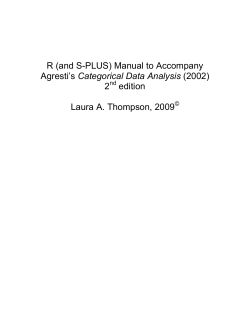
5.4. Forest Fires
The forest п¬Ѓre data were collected during January 2000 to December 2003 for п¬Ѓres in the
Montesinho natural park located in the Northeast region of Portugal. The response variable
of interest was area burned in ha. When the area burned as less than one-tenth of a hectare,
the response variable as set to zero. In all there were 517 п¬Ѓres and 247 of them recorded as
zero.
stered, such
the time,and
date,Morais
'V atiallocation
9 X9 п¬Ѓt
gn d
(" and
yams
The datasetwere
wasregtprovided
byasCortez
(2007)within
who aalso
this
data
using neural
of Figure 2), the type of vegetation involved, the SiX components of the FWI system
nets and support
machines.
total burned
,.-ea. The second database wa; collected by the Brag,."a Polyand the vector
technic Institute, containing several weather observations (eg wind speed) that were
The region recorded
was divided
a 10-by-10
coordinates
X loc<ted
and Ymrunning
from 1 to 9
with ainto
30 mmute
penod grid
by a with
meteorologtcal
station
the center
of the Montesmho park. The two databases were stored m tens ofmdividual 'Vreadas shown insheets,
the diagram
below. Theand
categorical
variable
region in this
under distinct
a substantial
manual xyarea
effort wa;indicates
perfonnedthe
to intemto a smgle datasetWlth a total of 517 entries. This d<tais availille at
grid for thegrate
п¬Ѓre.them
There
are 36 different regions so xyarea has 35 df.
fonn<t~
http.llwww.dsi.uminho.pt/~pcortez/forestfires/
F~2.
The map oftheMonte>inho n.tural pork
Figure 2: Montesinho Park
Table I shows a descnption ofthe selected data features. The first four rows denote
the spatial and temporal attributes. Only two geogr~hic features were mc1uded, the
X ,.,d Y axlS values where the fire occurred, Slnce the type of vegetation presented a
low quality (i. e. more than 80% 0f the values were mlSsmg). After consulting the M ontesmho fire mspector, we selected the month,.,d day of the week temporal vanables
Average monthly weather conditions are quite di stinc~ vJ1ile the day 0f the week coul d
also mfluence forest fires (e.g. work days vs weekend) smce most fires have a human
cause. Next come the four FWI components thit are affected directly by the weather
conditions (Figure I, m bold). The BUI and FWI were discarded smce they,.-e dependent of the previous values. From the meteorological station d<tabase, we selected the
four weather attributes used by the FWI system. In contrast with the time lags used by
FWI, m this case the values denote mst,.,trecords, as given by the station sensors when
the fire was detected. The exception lS the rain vanable, which denotes the occumulated
preapilati on within the prevIOus 30 mmutes
Fitting the best-AIC regression,
R> data(Fires)
R> bestglm(Fires, IC = "AIC")
26
bestglm: Best Subset GLM
Morgan-Tatar search since factors present with more than 2 levels.
AIC
Best Model:
Df Sum Sq Mean Sq F value Pr(>F)
month
11 37.37 3.3970 1.7958 0.05195 .
DMC
1
6.31 6.3145 3.3381 0.06829 .
DC
1
4.85 4.8468 2.5622 0.11008
temp
1
8.92 8.9165 4.7136 0.03039 *
wind
1
3.94 3.9384 2.0820 0.14967
Residuals
501 947.72 1.8917
--Signif. codes: 0 '***' 0.001 '**' 0.01 '*' 0.05 '.' 0.1 ' ' 1
6. Simulated Data
6.1. Null Regression Example
Here we check that our function handles the null regression case where there are no inputs to
include in the model. We assume an intercept term only.
R>
R>
R>
R>
R>
set.seed(123312123)
X <- as.data.frame(matrix(rnorm(50), ncol = 2, nrow = 25))
y <- rnorm(25)
Xy <- cbind(X, y = y)
bestglm(Xy)
BIC
BICq equivalent for q in (0, 0.540989544689166)
Best Model:
Estimate Std. Error
t value Pr(>|t|)
(Intercept) -0.3074955 0.2323344 -1.323504 0.1981378
6.2. Logistic Regression
As a check we simulate a logistic regression with рќђѕ = 10 inputs. The inputs are all Gaussian
white noise with unit variance. So the model equation may be written, рќ‘Њ is IID Bernouilli
distribution with parameter рќ‘ќ, рќ‘ќ = в„°(рќ‘Њ ) = в„Ћ(рќ›Ѕ0 + рќ›Ѕ1 рќ‘‹1 + . . . + рќ›Ѕрќђѕ рќ‘‹рќђѕ ) where в„Ћ(рќ‘Ґ) =
(1 + рќ‘’в€’рќ‘Ґ )в€’1 . Note that в„Ћ is the inverse of the logit transformation and it may coveniently
obtained in R using plogist. In the code below we set рќ›Ѕ0 = рќ‘Ћ = в€’1 and рќ›Ѕ1 = 3, рќ›Ѕ2 = 2,
рќ›Ѕ3 = 4/3, рќ›Ѕ4 = 2 32 and рќ›Ѕрќ‘– = 0, рќ‘– = 5, . . . , 10. Taking рќ‘› = 500 as the sample size we п¬Ѓnd after
п¬Ѓt with glm.
R> set.seed(231231)
R> n <- 500
A. I. McLeod, C. Xu
R>
R>
R>
R>
R>
R>
R>
R>
R>
R>
27
K <- 10
a <- -1
b <- c(c(9, 6, 4, 8)/3, rep(0, K - 4))
X <- matrix(rnorm(n * K), ncol = K)
L <- a + X %*% b
p <- plogis(L)
Y <- rbinom(n = n, size = 1, prob = p)
X <- as.data.frame(X)
out <- glm(Y Лњ ., data = X, family = binomial)
summary(out)
Call:
glm(formula = Y Лњ ., family = binomial, data = X)
Deviance Residuals:
Min
1Q
Median
-2.80409 -0.28120 -0.02809
3Q
0.25338
Max
2.53513
Coefficients:
Estimate Std. Error z value Pr(>|z|)
(Intercept) -0.882814
0.182554 -4.836 1.33e-06 ***
V1
3.186252
0.325376
9.793 < 2e-16 ***
V2
1.874106
0.242864
7.717 1.19e-14 ***
V3
1.500606
0.215321
6.969 3.19e-12 ***
V4
2.491092
0.281585
8.847 < 2e-16 ***
V5
0.029539
0.165162
0.179
0.858
V6
-0.179920
0.176994 -1.017
0.309
V7
-0.047183
0.172862 -0.273
0.785
V8
-0.121629
0.168903 -0.720
0.471
V9
-0.229848
0.161735 -1.421
0.155
V10
-0.002419
0.177972 -0.014
0.989
--Signif. codes: 0 '***' 0.001 '**' 0.01 '*' 0.05 '.' 0.1 ' ' 1
(Dispersion parameter for binomial family taken to be 1)
Null deviance: 685.93
Residual deviance: 243.86
AIC: 265.86
on 499
on 489
degrees of freedom
degrees of freedom
Number of Fisher Scoring iterations: 7
6.3. Binomial Regression
As a further check we п¬Ѓt a binomial regression taking рќ‘› = 500 with рќђѕ = 10 inputs and
with Bernouilli number of trials рќ‘љ = 100. So in this case the model equation may be
28
bestglm: Best Subset GLM
written, рќ‘Њ is IID binomially distributed with number of trials рќ‘љ = 10 and parameter рќ‘ќ,
𝑝 = ℰ(𝑌 ) = ℎ(𝛽0 + 𝛽1 𝑋1 + . . . + 𝛽𝐾 𝑋𝐾 ) where ℎ(𝑥) = (1 + 𝑒−𝑥 )−1 . We used the same 𝛽’s as
in Section 6.2.
R>
R>
R>
R>
R>
R>
R>
R>
R>
R>
R>
R>
R>
R>
R>
set.seed(231231)
n <- 500
K <- 8
m <- 100
a <- 2
b <- c(c(9, 6, 4, 8)/10, rep(0, K - 4))
X <- matrix(rnorm(n * K), ncol = K)
L <- a + X %*% b
p <- plogis(L)
Y <- rbinom(n = n, size = m, prob = p)
Y <- cbind(Y, m - Y)
dimnames(Y)[[2]] <- c("S", "F")
X <- as.data.frame(X)
out <- glm(Y Лњ ., data = X, family = binomial)
summary(out)
Call:
glm(formula = Y Лњ ., family = binomial, data = X)
Deviance Residuals:
Min
1Q
-2.77988 -0.70691
Median
0.07858
3Q
0.75158
Max
2.70323
Coefficients:
Estimate Std. Error z value Pr(>|z|)
(Intercept) 2.025629
0.016967 119.383
<2e-16 ***
V1
0.898334
0.015175 59.197
<2e-16 ***
V2
0.607897
0.012987 46.809
<2e-16 ***
V3
0.429355
0.013609 31.551
<2e-16 ***
V4
0.835002
0.014962 55.807
<2e-16 ***
V5
-0.006607
0.013867 -0.476
0.634
V6
-0.011497
0.013596 -0.846
0.398
V7
0.022112
0.013660
1.619
0.105
V8
0.000238
0.013480
0.018
0.986
--Signif. codes: 0 '***' 0.001 '**' 0.01 '*' 0.05 '.' 0.1 ' ' 1
(Dispersion parameter for binomial family taken to be 1)
Null deviance: 10752.23
Residual deviance:
507.19
AIC: 2451.8
on 499
on 491
degrees of freedom
degrees of freedom
A. I. McLeod, C. Xu
29
Number of Fisher Scoring iterations: 4
In this example, one input V6 is signficant at level 0.03 even though its correct coefficient is
zero.
R> Xy <- cbind(X, Y)
R> bestglm(Xy, family = binomial)
Morgan-Tatar search since family is non-gaussian.
BIC
BICq equivalent for q in (0, 0.870630550022155)
Best Model:
Estimate Std. Error
z value
Pr(>|z|)
(Intercept) 2.0247237 0.01689493 119.84211 0.000000e+00
V1
0.8995804 0.01513694 59.42948 0.000000e+00
V2
0.6063199 0.01287612 47.08872 0.000000e+00
V3
0.4290062 0.01360140 31.54132 2.358219e-218
V4
0.8349437 0.01485556 56.20412 0.000000e+00
Using the default selection method, BIC, the correct model is selected.
6.4. Binomial Regression With Factor Variable
An additional check was done to incorporate a factor variable. We include a factor input
representing the day-of-week effect. The usual corner-point method was used to parameterize
this variable and large coefficients chosen, so that this factor would have a strong effect. Using
the corner-point method, means that the model matrix will have six additional columns of
indicator variables. We used four more columns of numeric variables and then added the six
columns for the indicators to simulate the model.
R>
R>
R>
R>
R>
R>
+
R>
R>
R>
R>
R>
R>
R>
R>
R>
set.seed(33344111)
n <- 500
K <- 4
m <- 100
a <- 2
dayNames <- c("Sunday", "Monday", "Tuesday", "Wednesday", "Friday",
"Saturday")
Days <- data.frame(d = factor(rep(dayNames, n))[1:n])
Xdays <- model.matrix(Лњd, data = Days)
bdays <- c(7, 2, -7, 0, 2, 7)/10
Ldays <- Xdays %*% bdays
b <- c(c(9, 6)/10, rep(0, K - 2))
X <- matrix(rnorm(n * K), ncol = K)
L <- a + X %*% b
L <- L + Ldays
p <- plogis(L)
30
R>
R>
R>
R>
R>
R>
R>
bestglm: Best Subset GLM
Y <- rbinom(n = n, size = m, prob = p)
Y <- cbind(Y, m - Y)
dimnames(Y)[[2]] <- c("S", "F")
X <- as.data.frame(X)
X <- data.frame(X, days = Days)
out <- glm(Y Лњ ., data = X, family = binomial)
anova(out, test = "Chisq")
Analysis of Deviance Table
Model: binomial, link: logit
Response: Y
Terms added sequentially (first to last)
Df Deviance Resid. Df Resid. Dev P(>|Chi|)
NULL
499
5609.2
V1
1 2992.36
498
2616.9
<2e-16 ***
V2
1 1253.89
497
1363.0
<2e-16 ***
V3
1
2.49
496
1360.5
0.1145
V4
1
1.91
495
1358.6
0.1668
d
5
797.44
490
561.1
<2e-16 ***
--Signif. codes: 0 '***' 0.001 '**' 0.01 '*' 0.05 '.' 0.1 ' ' 1
After fitting with glm we find the results as expected. The factor variable is highly signficant
as well as the п¬Ѓrst two quantiative variables.
Using bestglm, we п¬Ѓnd it selects the correct model.
R> Xy <- cbind(X, Y)
R> out <- bestglm(Xy, IC = "BICq", family = binomial)
Morgan-Tatar search since family is non-gaussian.
Note: factors present with more than 2 levels.
R> out
BICq(q = 0.25)
Best Model:
Response S :
Df Sum Sq Mean Sq F value
Pr(>F)
V1
1 24841.5 24841.5 792.61 < 2.2e-16 ***
V2
1 9110.0 9110.0 290.67 < 2.2e-16 ***
d
5 7473.4 1494.7
47.69 < 2.2e-16 ***
A. I. McLeod, C. Xu
Residuals
492 15419.9
31.3
--Signif. codes: 0 '***' 0.001 '**' 0.01 '*' 0.05 '.' 0.1 ' ' 1
Response F :
Df Sum Sq Mean Sq F value
V1
1 24841.5 24841.5 792.61
V2
1 9110.0 9110.0 290.67
d
5 7473.4 1494.7
47.69
Residuals
492 15419.9
31.3
--Signif. codes: 0 '***' 0.001 '**' 0.01
Pr(>F)
< 2.2e-16 ***
< 2.2e-16 ***
< 2.2e-16 ***
'*' 0.05 '.' 0.1 ' ' 1
6.5. Poisson Regression
R>
R>
R>
R>
R>
R>
R>
R>
R>
R>
R>
R>
set.seed(231231)
n <- 500
K <- 4
a <- -1
b <- c(c(1, 0.5), rep(0, K - 2))
X <- matrix(rnorm(n * K), ncol = K)
L <- a + X %*% b
lambda <- exp(L)
Y <- rpois(n = n, lambda = lambda)
X <- as.data.frame(X)
out <- glm(Y Лњ ., data = X, family = poisson)
summary(out)
Call:
glm(formula = Y Лњ ., family = poisson, data = X)
Deviance Residuals:
Min
1Q
Median
-2.1330 -0.8084 -0.4853
3Q
0.4236
Max
2.6320
Coefficients:
Estimate Std. Error z value Pr(>|z|)
(Intercept) -0.92423
0.07933 -11.650
<2e-16 ***
V1
0.97841
0.05400 18.119
<2e-16 ***
V2
0.51967
0.05707
9.107
<2e-16 ***
V3
0.03773
0.05525
0.683
0.495
V4
0.03085
0.04646
0.664
0.507
--Signif. codes: 0 '***' 0.001 '**' 0.01 '*' 0.05 '.' 0.1 ' ' 1
31
32
bestglm: Best Subset GLM
(Dispersion parameter for poisson family taken to be 1)
Null deviance: 880.73
Residual deviance: 427.49
AIC: 913.41
on 499
on 495
degrees of freedom
degrees of freedom
Number of Fisher Scoring iterations: 5
As expected the first two variables are highly signficant and the next two are not.
R> Xy <- data.frame(X, y = Y)
R> bestglm(Xy, family = poisson)
Morgan-Tatar search since family is non-gaussian.
BIC
BICq equivalent for q in (0, 0.947443940310683)
Best Model:
Estimate Std. Error
z value
Pr(>|z|)
(Intercept) -0.9292265 0.07955966 -11.679619 1.620199e-31
V1
0.9897770 0.05284046 18.731421 2.744893e-78
V2
0.5302822 0.05588287
9.489171 2.328782e-21
Our function bestglm selects the correct model.
6.6. Gamma Regression
To simulate a Gamma regression we п¬Ѓrst write a function GetGammaParameters that translates
mean and standard deviation into the shape and scale parameters for the function rgamma.
R> GetGammaParameters <- function(muz, sdz) {
+
phi <- (sdz/muz)Л†2
+
nu <- 1/phi
+
lambda <- muz/nu
+
list(shape = nu, scale = lambda)
+ }
R> set.seed(321123)
R> test <- rnorm(20)
R> n <- 500
R> b <- c(0.25, 0.5, 0, 0)
R> b0 <- 0.3
R> K <- length(b)
R> sdz <- 1
R> X <- matrix(rnorm(n * K), ncol = K)
R> L <- b0 + X %*% b
R> muHat <- exp(L)
R> gp <- GetGammaParameters(muHat, sdz)
R> zsim <- rgamma(n, shape = gp$shape, scale = gp$scale)
A. I. McLeod, C. Xu
33
R> Xy <- data.frame(as.data.frame.matrix(X), y = zsim)
R> out <- glm(y Лњ ., data = Xy, family = Gamma(link = log))
R> summary(out)
Call:
glm(formula = y Лњ ., family = Gamma(link = log), data = Xy)
Deviance Residuals:
Min
1Q
Median
-5.6371 -0.7417 -0.1968
3Q
0.2237
Max
3.2105
Coefficients:
Estimate Std. Error t value
(Intercept) 0.313964
0.044124
7.115
V1
0.191957
0.040983
4.684
V2
0.558321
0.042485 13.142
V3
0.018709
0.044939
0.416
V4
0.004252
0.043367
0.098
--Signif. codes: 0 '***' 0.001 '**' 0.01
Pr(>|t|)
3.93e-12 ***
3.64e-06 ***
< 2e-16 ***
0.677
0.922
'*' 0.05 '.' 0.1 ' ' 1
(Dispersion parameter for Gamma family taken to be 0.944972)
Null deviance: 792.56
Residual deviance: 621.67
AIC: 1315.9
on 499
on 495
degrees of freedom
degrees of freedom
Number of Fisher Scoring iterations: 9
R> bestglm(Xy, family = Gamma(link = log))
Morgan-Tatar search since family is non-gaussian.
BIC
BICq equivalent for q in (0.000599916119599198, 0.953871171759292)
Best Model:
Estimate Std. Error
t value
Pr(>|t|)
(Intercept) 0.3110431 0.04353445 7.144757 3.229210e-12
V1
0.1931868 0.04098936 4.713096 3.172312e-06
V2
0.5560244 0.04226866 13.154531 4.011556e-34
As expected, bestglm selects the correct model.
7. Simulation Experiment
Please see the separate vignette Xu and McLeod (2009) for a discussion of how the simulation
experiment reported in Xu and McLeod (2010, Table 2) was carried out as well for more
34
bestglm: Best Subset GLM
detailed results of the simulation results themselves. The purpose of the simulation experiment reported on in Xu and McLeod (2010, Table 2) and described in more detail in the
accompanying vignette Xu and McLeod (2009) was to compare different information criteria
used in model selection.
Similar simulation experiments were used by Shao (1993) to compare cross-valiation criteria
for linear model selection. In the simulation experiment reported by Shao (1993), the performance of various CV methods for linear model selection were investigated for the linear
regression,
𝑦 = 2 + 𝛽2 𝑥2 + 𝛽3 𝑥3 + 𝛽4 𝑥4 + 𝛽5 𝑥5 + 𝑒,
(8)
where рќ‘’ nid(0, 1). A п¬Ѓxed sample size of рќ‘› = 40 was used and the design matrix used is given
in (Shao 1993, Table 1) and the four different values of the 𝛽’s are shown in the table below,
Experiment рќ›Ѕ2 рќ›Ѕ3 рќ›Ѕ4 рќ›Ѕ5
1
0
0
4
0
2
0
0
4
8
3
9
0
4
8
4
9
6
4
8
The table below summarizes the probability of correct model selection in the experiment
reported by Shao (1993, Table 2). Three model selection methods are compared: LOOCV
(leave-one-out CV), CV(d=25) or the delete-d method with d=25 and APCV which is a very
efficient computation CV method but specialized to the case of linear regression.
Experiment LOOCV CV(d=25) APCV
1 0.484
0.934
0.501
2 0.641
0.947
0.651
3 0.801
0.965
0.818
4 0.985
0.948
0.999
The CV(d=25) outperforms LOOCV in all cases and it also outforms APCV by a large margin
in Experiments 1, 2 and 3 but in case 4 APCV is slightly better.
In the code below we show how to do our own experiments to compare model selection using
the bic, bicрќ›ѕ and bicрќ‘ћ criteria.
R> testCorrect <- function(ans, NB) {
+
NBfit <- names(coef(ans))[-1]
+
ans <- ifelse(length(NBfit) == length(NB) & (!any(is.na(match(NBfit,
+
NB)))), 1, 0)
+
ans
+ }
R> NSIM <- 5
R> data(Shao)
R> set.seed(123321123)
R> X <- as.matrix.data.frame(Shao)
R> BETA <- list(b1 = c(0, 0, 4, 0), b2 = c(0, 0, 4, 8), b3 = c(9,
+
0, 4, 8), b4 = c(9, 6, 4, 8))
R> NamesBeta <- list(b1 = c("x4"), b2 = c("x4", "x5"), b3 = c("x2",
+
"x4", "x5"), b4 = c("x2", "x3", "x4", "x5"))
R> hitsBIC <- hitsEBIC <- hitsQBIC <- numeric(4)
A. I. McLeod, C. Xu
35
R> startTime <- proc.time()[1]
R> for (iB in 1:4) {
+
b <- BETA[[iB]]
+
NB <- NamesBeta[[iB]]
+
for (iSIM in 1:NSIM) {
+
y <- 2 + X %*% b + rnorm(40)
+
Xy <- cbind(Shao, y)
+
hitsBIC[iB] <- hitsBIC[iB] + testCorrect(bestglm(Xy,
+
IC = "BIC")$BestModel, NB)
+
hitsEBIC[iB] <- hitsEBIC[iB] + testCorrect(bestglm(Xy,
+
IC = "BICg")$BestModel, NB)
+
hitsQBIC[iB] <- hitsQBIC[iB] + testCorrect(bestglm(Xy,
+
IC = "BICq")$BestModel, NB)
+
}
+ }
R> endTime <- proc.time()[1]
R> totalTime <- endTime - startTime
R> ans <- matrix(c(hitsBIC, hitsEBIC, hitsQBIC), byrow = TRUE, ncol = 4)
R> dimnames(ans) <- list(c("BIC", "BICg", "BICq"), 1:4)
R> ans <- t(ans)/NSIM
R> ans
1
2
3
4
BIC BICg BICq
0.6 0.8 0.8
1.0 0.8 1.0
1.0 0.8 1.0
1.0 1.0 1.0
R> totalTime
user.self
1.01
Increasing the number of simulations so NSIM=10000, the following result was obtained,
1
2
3
4
BIC
0.8168
0.8699
0.9314
0.9995
BICg
0.8666
0.7741
0.6312
0.9998
BICq
0.9384
0.9566
0.9761
0.9974
8. Controlling Type 1 Error Rate
Consider the case where there are рќ‘ќ input variables and it we wish to test the null hypothesis
в„‹0 : the output is not related to any inputs. By adjusting рќ‘ћ in the bicрќ‘ћ criterion, we can
control the Type 1 error rate. Using simulation, we can determine for any particular рќ‘› and
36
bestglm: Best Subset GLM
рќ‘ќ, what value of рќ‘ћ is needed to achieve a Type 1 error rate for a particular level, such as
рќ›ј = 0.05.
We compare the performance of information selection criteria in the case of a null model with
рќ‘ќ = 25 inputs and рќ‘› = 30 observations. Using 50 simulations takes about 30 seconds. Since
there is no relation between the inputs and the output, the correct choice is the null model
with no parameters. Using the BICq criterion with рќ‘ћ = 0.05 works better than AIC, BIC or
BICg. We may consider the number of parameters selected as the frequency of Type 1 errors
in an hypothesis testing framework. By adjusting рќ‘ћ we may adjust the Type 1 error rate to
any desired level. This suggests a possible bootstrapping approach to the problem of variable
selection.
R> set.seed(123321123)
R> startTime <- proc.time()[1]
R> NSIM <- 5
R> p <- 25
R> n <- 30
R> ans <- numeric(4)
R> names(ans) <- c("AIC", "BIC", "BICg", "BICq")
R> for (iSim in 1:NSIM) {
+
X <- matrix(rnorm(n * p), ncol = p)
+
y <- rnorm(n)
+
Xy <- as.data.frame(cbind(X, y))
+
names(Xy) <- c(paste("X", 1:p, sep = ""), "y")
+
bestAIC <- bestglm(Xy, IC = "AIC")
+
bestBIC <- bestglm(Xy, IC = "BIC")
+
bestEBIC <- bestglm(Xy, IC = "BICg")
+
bestQBIC <- bestglm(Xy, IC = "BICq", t = 0.05)
+
ans[1] <- ans[1] + length(coef(bestAIC$BestModel)) - 1
+
ans[2] <- ans[2] + length(coef(bestBIC$BestModel)) - 1
+
ans[3] <- ans[3] + length(coef(bestEBIC$BestModel)) - 1
+
ans[4] <- ans[4] + length(coef(bestQBIC$BestModel)) - 1
+ }
R> endTime <- proc.time()[1]
R> totalTime <- endTime - startTime
R> totalTime
user.self
4.52
R> ans
AIC
58
BIC BICg BICq
13
0
0
9. Concluding Remarks
A. I. McLeod, C. Xu
37
The subset regression problem is related to the subset autoregression problem that as been
discussed by McLeod and Zhang (2006, 2008) and implemented in the FitAR R package
available on CRAN. The FitAR has been updated to include the new bicрќ‘ћ criterion.
References
Akaike H (1970). “Statistical Predictor Identification.” Annals of the Institute of Statistical
Mathematics, 22, 203–217.
Akaike H (1974). “A new look at the statistical model identification.” IEEE Trans. Automatic
Control, 19(6), 716–723.
Allen DM (1971). “Mean square error of prediction as a criterion for selecting variables.”
Technometrics, 13, 459–475.
Breiman L, Freidman JH, Olshen RA, Stone CJ (1984). Classification and Regression Trees.
Wadsworth.
Brusco MJ, Stahl S (2009). Branch-and-Bound Applications in Combinatorial Data Analysis.
Springer-Verlag, New York.
Cadima J, Cerdeira J, Orestes J, Minhoto M (2004). “Computational aspects of algorithms
for variable selection in the context of principal components.” Computational Statistics and
Data Analysis, 47, 225–236.
Cerdeira JO, Silva PD, Cadima J, Minhoto M (2009). subselect: Selecting Variable Subsets.
R package version 0.9-9993, URL http://CRAN.R-project.org/package=subselect.
Chen J, Chen Z (2008). “Extended Bayesian Information Criteria for Model Selection with
Large Model Space.” Biometrika, 95, 759–771.
Cortez P, Morais A (2007). “A Data Mining Approach to Predict Forest Fires using Meteorological Data.” In MFS J Neves, J Machado (eds.), “New Trends in Artificial Intelligence,” volume Proceedings of the 13th EPIA 2007, pp. 512–523. Portuguese Conference
on Artificial Intelligence, Guimar˜
aes, Portugal. ISBN 13 978-989-95618-0-9. The paper is
available from: http://www3.dsi.uminho.pt/pcortez/fires.pdf and the dataset from:
http://archive.ics.uci.edu/ml/datasets/Forest+Fires.
Davison AC, Hinkley DV (1997). Bootstrap Methods and Their Applications. Cambridge
University Press, Cambridge.
Gatu C (2006). “Branch-and-Bound Algorithms for Computing the Best-Subset Regression
Models.” Journal of Computational and Graphical Statistics, 15, 139–156.
Granger C, Jeon Y (2004). “Forecasting Performance of Information Criteria with Many
Macro Series.” Journal of Applied Statistics, 31, 1227–1240.
Hastie T, Tibshirani R, Friedman J (2009). The Elements of Statistical Learning: Data
Mining, Inference and Prediction. Springer-Verlag, New York, 2nd edition.
38
bestglm: Best Subset GLM
Hosmer DW, Jovanovic B, Lemeshow S (1989). “Best Subsets Logistic Regression.” Biometrics, 45(4), 1265–1270.
Knuth DE (2005). The Art of Computer Programming, volume 4. Addison-Wesley, Upper
Saddle River.
Koehler AB, Murphree ES (1988). “A Comparison of the Akaike and Schwarz Criteria for
Selecting Model Order.” Applied Statistics, 37(2), 187–195. ISSN 00359254.
Lumley T, Miller A (2004). leaps: Regression Subset Selection. R package version 2.7, URL
http://CRAN.R-project.org/package=leaps.
Mallows CL (1973). “Some Comments on C𝑝 .” Technometrics, 15, 661–675.
McLeod AI, Zhang Y (2006). “Partial Autocorrelation Parameterization for Subset Autoregression.” Journal of Time Series Analysis, 27, 599–612.
McLeod AI, Zhang Y (2008). “Improved Subset Autoregression: With R Package.” Journal
of Statistical Software, 28(2), 1–28. URL http://www.jstatsoft.org/v28/i02.
Miller AJ (2002). Subset Selection in Regression. Chapman & HallCRC, Boca Raton, 2nd
edition.
Morgan JA, Tatar JF (1972). “Calculation of the Residual Sum of Squares for all Possible
Regressions.” Technometrics, 14, 317–325.
Nishii R (1984). “Asymptotic Properties of Criteria for Selection of Variables in Multiple
Regression.” The Annals of Statistics, 12, 758–765.
Noakes DJ, McLeod AI, Hipel KW (1985). “Forecasting seasonal hydrological time series.”
The International Journal of Forecasting, 1, 179–190.
Percival DB, Walden AT (1993). Spectral Analysis For Physical Applications. Cambridge
University Press, Cambridge.
Rencher AC, Fu CP (1980). “Inflation of 𝑅2 in Best Subset Regression.” Technometrics, 22,
49–53.
Schwarz G (1978). “Estimation the Dimension of a Model.” Annals of Statistics, 6, 461–464.
Shao J (1993). “Linear Model Selection by Cross-Validation Linear Model Selection by CrossValidation.” Journal of the American Statistical Association, 88, 486–494.
Shao J (1997). “An asymptotic theory for linear model selection.” Statistica Sinica, 7, 221–262.
Shibata R (1981). “An optimal selection of regression variables.” Biometrika, 68, 45–54. Corr:
V69 p492.
Stone M (1977). “An asymptotic equivalence of choice of model by cross-validation and
Akaike’s criterion.” Journal of the Royal Statistical Society, Series B, 39, 44–47.
Wilkinson L, Gerard ED (1981). “Tests of Significance in Forward Selection Regression with
an F-to-Enter Stopping Rule.” Technometrics, 23, 377–380.
A. I. McLeod, C. Xu
39
Xu C, McLeod AI (2009). “Linear Model Selection Using the BIC𝑞 Criterion.” Vignette
included in bestglm package, The University of Western Ontario.
Xu C, McLeod AI (2010). “Bayesian Information Criterion with Bernoulli prior.” Submitted
for publication.
Affiliation:
A.I. McLeod
University of Western Ontario
E-mail: [email protected]
Changjiang Xu
University of Western Ontario
E-mail: [email protected]
© Copyright 2026 Paperzz