Optimisation and Inverse Problems in Imaging
Simon R. Arridge
March 4, 2015
† Department of Computer Science, University College London, Gower Street London, WC1E 6BT
GV08
2007-2014
1
1
Introduction
The topic of Optimisation covers many areas. In this course we are going to consider the role of
Optimisation in imaging. In particular (but not exclusively) we are going to consider the role of
optimisation in the topic of Inverse Problems, and within this subject we are going to consider in
particular (but not exclusively) the topic of Inverse Problems in Imaging.
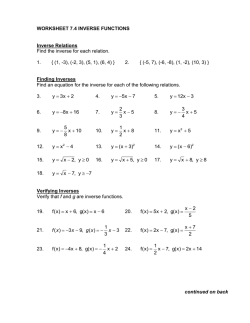
Broadly speaking Optimisation requires us to consider four things
• A metric. This addresses the question “Optimisation of what?”. A metric is a single real
positive number that acts as a “figure of merit” of our success at optimisation.
• A model . This addresses the question “what is the metric applied to?”. A model is a
mathematical or computational process that predicts a result which maybe a function, vector,
list or some other quantity.
• Parameters. This addresses the question “Optimisation over what ?”. These are the variable
controls of the model. The aim of optimisation is to adjust the parameters until the figure
of metric is in some way “as good as we can get”
• An algorithm. This addresses the question “How do we optimise?”
−1
yobserved
y noise−free
A
X
A(x)
xrecon
xtrue
Y
Figure 1.1:
2
There are many generalisations. We may sometimes consider not one but multiple metrics. An
important type of optimisation is model-fitting. In this case we need a 5th concept: Data. In
this case the metric is not just applied to the model, but to the model and the data together to
evaluate how well the model predicts the data.
2
2.1
2.1.1
Basic Concepts
Some examples
Minimum norm solutions to Underdetermined Problems
Consider the following problem : Solve
x1 + 2x2 = 5
(2.1)
There is no unique solution. The set of possible solutions forms a line on the x1 , x2 plane. However
the following can be solved :
Φ = x21 + x22
x1 + 2x2 = 5
minimise
subject to
(2.2)
which has solution (x1 , x2 ) = (1, 2). It is illustrated graphically in figure 2.1. This is an example
x2
x1 + 2 x2= 5
(1,2)
x1
x21 + x22 = constant
Figure 2.1:
of constrained optimisation. The unique solution is the one where the surface Φ = constant is
tangent to the constraint x1 + 2x2 = 5. The expression Φ = x21 + x22 is a norm (i.e. a metric, or
ˆ 1 = (1, 0), x
ˆ 2 = (0, 1). In this
distance measure) on the Euclidean space R2 with basis vectors x
3
case, because the norm is quadratic, the solution is found by taking the Moore-Penrose generalised
inverse of the underdetermined linear equation Eq. 2.1 :
−1
x1
1
1
1
=
(12)
(5) =
(2.3)
x2
2
2
2
and the solution is the minimum norm solution, where the norm is the normal Euclidean L2 norm.
Now consider that we take a different norm and ask for the solution to
Φ = xp1 + xp2
x1 + 2x2 = 5 .
minimise
subject to
(2.4)
When 1 < p < ∞ the surfaces Φ = constant are convex and solutions can be found relatively
easily. We see that we can obtain any solution between (0, 2.5) at p = 1 and (1 32 , 1 32 ) for p = ∞.
x2
8
8
x1 + 2 x2= 5
x1 + x2 = constant
(0,2.5)
(1,2)
(1.67,1.67)
x1
x21 + x22 = constant
|x1|+ |x2 |= constant
Figure 2.2:
However, actually calculating the solution is not as simple as solving a linear problem like Eq. 2.3.
The case p = 1 is known as the sparse solution.
The case 0 < p < 1 leads to concave surfaces and to the more complex problem of non-convex
optimisation.
4
270
260
250
240
230
220
210
200
190
180
170
80
85
90
95
100
105
110
Figure 2.3: Fitting polynomials of increasing order to a set of points
2.1.2
Model Fitting
Suppose we have a set of data {xi , yi ; i = 1 . . . N} and a hypothetical model
y = A(x; ξ)
parameterised by values {ξ0 , ξ1, ...ξM }. We can provide a fit of the model by optimising a data
fitting function such as
N
1X
|yi − A(xi , ξ)|2
(2.5)
Φ=
2 i=1
see figure 2.3. More generally, we may define a data-fitting functional
Φ = D(y, A(x, ξ)) .
(2.6)
This framework admits, for example, the p-norms we introduced in Eq.(2.4), or they may be
more general norms such as Kullback-Liebeck divergence, or Cross-entropy. In general the choice
of norm in the space of the data is dicated by the expected statistics of the errors in the data.
A choice of the L2 norm corresponds to assuming identically distributed, independent Gaussian
random variable for the errors (iid Normal distributions).
If the model is linear, and the data-fitting functional is sum of squares the problem is linear
least-squares and can be solved using linear algebra. For example, fitting a cubic polynomial
y = ξ0 + ξ1 x + ξ2 x2 + ξ3 x3 to N > 4 data is an over-determined problem defined by
  
 
y1
1 x1 x21 x31
ξ0
 y2  1 x2 x2 x3   
2
2  ξ1 
  
(2.7)
 ..  =  .. ..
..
..  ξ 
 .  . .
.
.  2
ξ3
yN
1 xN x2N x3N
5
If A is non-linear with respect to the parameters ξ then the process is one of non-linear, unconstrained optimisation. This could be non-linear least-squares, or a more general problem.
2.1.3
Inequality constraints
Consider the same problem as in section 2.1.1, but introduce bound on the solution
Φ = x21 + x22
x1 + 2x2 = 5
2 ≤ x1 ≤ 4
1 ≤ x2 ≤ 5
minimise
subject to
(2.8)
(2.9)
which has solution (x1 , x2 ) = (2, 1.5), see figure 2.4. Unlike Eq. 2.2 this cannot be solved by a
x2
x1 + 2 x2= 5
(2,1.5)
x1
x21 + x22 = constant
Figure 2.4:
simple linear method like Eq. 2.3.
References for this section
[1, 2, 3, 4]
2.2
2.2.1
Inverse Problems
Problem 1 : Non Uniqueness
Solve
x1 + x2 = 2
6
(2.10)
This problem has an infinite number of solutions. The set of equations are underdetermined. To
find a single solution we need to add constraints and use a constrained optimisation method.
2.2.2
Problem 2 : Non Existence
Solve
x1 = 1
x1 = 3
(2.11)
This problem has no solution. The set of equations are overdetermined. We can find a possible
solution using unconstrained optimisation. Consider the following problem :
Φ = (x1 − 1)2 + (x1 − 3)2 → min
(2.12)
It is easy to see we cannot get a solution with Φ = 0 because we can solve a quadratic equation
exactly
(x1 − 1)2 + (x2 − 3)2 = 0
⇒ 2x21 − 8x1 + 10 = 0
√
4 ± 16 − 20
⇒ x1 =
2
= 2 ± 2i
i.e. the solution has no real roots. Instead we can find the minimum :x1 = 2, Φ = 2. This is the
least squares solution.
2.2.3
Problem 3 : Discontinuous dependence on data
Solve
Ax =
1
1+ǫ
1−ǫ
1
1
x1
=
2
x2
(2.13)
This problem has a solution that tends towards instability. There are a number of ways to see
this. The matrix A has determinant ǫ2 so its inverse is
1
1
−(1 + ǫ)
−1
(2.14)
A = 2
1
ǫ −(1 − ǫ)
Thus the inverse grows as an inverse square in the parameter ǫ.
To see the effect of the inverse with respect to noise, consider the following example :
Results are shown in figure 2.2.3. We see that the data has an isotropic distribution around
the specified noise free point whereas the solution has a highly non-isotropic distribution. This
7
Algorithm 1 Statistical trial of ill-posed matrix inversion
for all trials i = 1 . . . N do
0
1 0
draw a random vector of length 2 with Gaussian probability ηi ∼ N
,
0
0 1
generate data bi = (10, 20) + ηi
solve Axi = bi
end for
24
450
23
400
22
350
21
20
300
19
250
18
200
17
16
6
8
10
12
150
−500
14
−400
−300
−200
−100
Figure 2.5: Results of ill-posed matrix inversion trial for ǫ ≃ 0.2.Left : The distribution of data
points. Right : the distribution of solutions. The singular values of the matrix are 2.02, 0.0202,
and the standard deviation of the covariance of the solution points are 1.9984, 0.020502
highly anisotropic amplification of noise preferentially in some directions is an example of the third
kind of ill-posedness of inverse problems. To understand the nature of this ill-posedness we can
investigate the structure of the linear forward problem using the Singular Value Decomposition
(SVD).
References for this section
[5]
2.3
Singular Value Decomposition (SVD)
The eigenvalues of A can be found by solving
λ2 − 2λ + ǫ2 = 0
⇒
λ=1±
√
1 − ǫ2 .
with corresponding eigenvectors (unnormalised)
√
√
1 − ǫ2
− 1 − ǫ2
e1 =
, e2 =
1−ǫ
1−ǫ
8
[NOTE : Since the matrix is not symmetric, the eigenvectors are not orthogonal]
Taking the limit of these solutions as ǫ → 0 we find the limiting values for the eigenvalues :
1
λ1 → 2 − ǫ ,
2
1
λ2 → ǫ
2
with corresponding eigenvectors
1
e1 →
,
1
−1
e2 →
1
[NOTE : In the limit the matrix is symmetric, so the limiting eigenvectors are orthogonal]
We may also take the Singular Value Decomposition (SVD); In Matlab :
eps = 0.01;
A = [1 1+eps; 1 - eps 1];
[U,W,V] = svd(A);
[Note that Matlab requires numerics. The symbolic part of Matlab is not very comprehensive]
We can write the SVD explicitly
√
√
1 ǫ − 1 + ǫ2
1 ǫ + 1 + ǫ2
, u2 =
u1 =
1
1
L+
L−
1/2
1/2
√
√
2
2
2
2
w1 = 2 + ǫ + 2 1 + ǫ
, w2 = 2 + ǫ − 2 1 + ǫ
√
√
1 − 1 + ǫ2 − ǫ
1
1 + ǫ2 − ǫ
, v2 =
v1 =
1
1
L−
L+
√
√
1/2
1/2
, and L− = 1 + (ǫ − 1 + ǫ2 )2
are normalisations ; [Note
where L+ = 1 + (ǫ + 1 + ǫ2 )2
that normalisation must be carried out for SVD to provide the correct mappings between left and
right spaces].
Exercise 1 Verify the above SVD. I.e. show
Av i = wi ui ,
AT ui = wi v i
i = 1, 2
The SVD provides an alternative way to express the matrix inverse, and works also for non square
matrices.
9
2.3.1
Properties of SVD for matrices
The SVD can be defined for any linear operator. To begin with we will consider matrices. The
SVD of any N × M matrix A can be written as a product
VT
W |{z}
U |{z}
A = |{z}
|{z}
N ×M
(2.15)
N ×N N ×M M ×M
The columns of U are orthonormal, as are the columns of V. I.e. if we consider





u1,1
u2,1
uN,1
 u1,2   u2,2 
 uN,2  





U = [u1 u1 . . . uN ] =  ..   ..  . . .  ..  
 .   . 
 . 
u1,N
u2,N
uN,N
and


v1,1
 v1,2 


V = [v 1 v 1 . . . v M ] =  .. 
 . 
v1,M
Then we have
ui · uj = δij
i, j ∈ [1 . . . N] ,


v2,1
 v2,2 


 ..  . . .
 . 
v2,M
v i · v j = δij


vM,1
 vM,2  


 ..  
 . 
vM,M
i, j ∈ [1 . . . M] .
The matrix W has a structure depending on whether N is greater than, equal to, or less than M.
If N = M, W is square, with diagonal elements Wi,i = wi , i = 1 . . . N
If N > M, W has a M × M diagonal matrix above N − M rows of zero :


w1 0 0 . . . 0
 0 w2 0 . . . 0 


 0 0 w3 . . . 0 

..
.. . .
.. 
 ..

.
.
.
. 
diag(w)
 .
W=
=

0
 0 0 0 . . . wM 


 0 0 0 ... 0 
 .
..
.. . .
.. 
 ..
.
.
.
. 
0 0 0 ... 0
10
If N < M, W has a N × N diagonal matrix to the left of M − N columns

w1 0 0 . . . 0 0 . . .
 0 w2 0 . . . 0 0 . . .


W = diag(w) 0 =  0 0 w3 . . . 0 0 . . .
 ..
.
.. . .
..
 .
. ..
.
.
0 0 0 . . . wN 0 . . .
of zero :

0
0

0



0
The number of non-zeros in the diagonal part of W is equal to the rank of the matrix A i.e. the
number of linearly independent columns (or rows) of the matrix
R = rank(A) ≤ min(N, M)
For convenience, assume that the linearly independent columns of U, V are arranged as the first
R components, and further that the indexing of columns is such that |wi | > |wi+1 |. The elements
of the diagonal part of W are termed the spectrum of A.
The R column-vectors of V corresponding to the non-zero elements of the diagonal of W form an
orthonormal basis spanning a R-dimensional vector space called the row-space, and the R columnvectors of U corresponding to these elements form an orthonormal basis spanning a R-dimensional
vector space called the range range(A) or column-space. These basis functions are related through
Av i = wi ui ,
AT ui = wi v i
i = 1...R
(2.16)
The remaining M − R column vectors of V (if greater than zero) form an orthonormal basis
spanning a M − R-dimensional vector space called the null-space Null(A), or kernel kern(A). For
any vector x⊥ ∈ Null(A) we have
Ax⊥ = 0
(2.17)
Similarly, the N −R column vectors of U (if greater than zero) form an orthonormal basis spanning
a N − R-dimensional vector space called the range complement range⊥ (A) or co-kernel. For any
vector b⊥ ∈ range⊥ (A) we have that the linear equation
Ax = b⊥
(2.18)
has no solutions.
For the simple case N = M = R the matrix A is square and full-rank and its inverse can be
expressed straightforwardly
A−1 = VW−1 UT
(2.19)
where W−1 is diagonal with components 1/wi , i = 1 . . . R. This representation allows to express
the solution of a particular problem
Ax = b → x =
11
R
X
ui · b
i=1
wi
vi
(2.20)
Now we can see a problem that is related to the third definition of an ill-posed problem given above
: even if A is full rank, if the relative magnitudes of the wi decrease rapidly, then the correponding
components of the inverse increase at the same rate. In particular, if the decay of the spectrum is
bounded by a geometric ratio then the inverse problem is termed exponentially ill-posed.
2.3.2
Pseudo-Inverse
The inverse matrix built from the row-space of A is called the Moore-Penrose pseudo-inverse of A.
A† = VW† UT =
R
X
v i uT
i
i=1
(2.21)
wi
Here W† is a M × N matrix with the complementary structure to W. To be specific :
†
If N = M = R, W† is square, with diagonal elements Wi,i
= 1/wi, i = 1 . . . N
If N > M, W† has a M × M diagonal matrix to the left of N − M columns of

1/w1
0
0
...
0
0...
 0
1/w2
0
...
0
0...

 0
†
0
1/w
.
.
.
0
0...
3
W = diag(w) 0 = 
 ..
..
..
.
.
..
..
 .
.
.
0
0
0
. . . 1/wM 0 . . .
If N < M, W† has a N × N diagonal matrix above M − N rows

1/w1
0
0
 0
1/w
0
2

 0
0
1/w3

..
..
 ..
.
.
diag(w)
 .
W† =
=
0
0
0
 0

0
0
 0
 .
.
..
..
 ..
.
0
0
0
zero :

0
0

0



0
of zero :
...
...
...
..
.
...
...
..
.
...
0
0
0
..
.








1/wN 

0 
.. 
. 
0
Exercise 2 Write down the stuctures of the matrices WW† and W† W for the cases N > M and
M < N and M = N. Assume for the sake of illustration that the rank R < min(M, N), i.e. that
there is a non-trivial null space and range complement space even in the case where M = N.
The pseudo-inverse can always be constructed regardless if A is non-square and/or rank-deficient.
Thus any linear matrix problem has a pseudo-solution
A x = b → x† = A† b
12
(2.22)
This solution has the property that it is the least-squares, minimum norm solution in the sense
that
|b − A x† | → min , |x† | → min
To see this, first we note :
I − AA† b
= U I − WW† UT b
= P⊥ b
b − Ax† =
where
P⊥ =
N
X
ui uT
i
(2.23)
i=R+1
is a matrix that projects data space vectors into the orthogonal complement of the range. Now
˜ = x† + x′ , with b′ = Ax′ the corresponding data space
consider another solution space vector x
vector, which by definition lies in the range of A. We have
|b − A˜
x| = |b − Ax† − Ax′ |
= |P⊥ b − UUT b′ |
N
R
X
X
2
2
=
(ui · b) +
(ui · b′ )
i=1
i=R+1
where the second sum on the right holds due to the fact that b′ ∈ Range(A). Thus any vector
x′ with a non-zero component in the Null-space of A will increase the data space norm. We now
need to see if any vector x′ ∈ Null(A) could give a smaller norm |˜
x|. We write
|˜
x| = |x† + x′ |
= |VW† UT b + VVT x′ |
= |V W† UT b + VT x′ |
= | W† UT b + VT x′ |
2
M
R X
X
ui · b
2
+
(v i · x′ )
=
wi
i=1
i=R+1
where the second sum on the right holds due to the fact that x′ ∈ Null(A). Thus any vector x′
with a non-zero component in the null-space of A will increase the solution space norm.
To complete our exposition, let us solve the three problems in section 2.2 using the pseudo-inverse.
13
2.3.3
Problem 1
A= 1 1
1
A =
2
†
⇒
SVD:
(1)
√
1
1
2 0
√1
2
− √12
√1
2
√1
2
!
1
x1
†
= A (2) =
⇒
1
x2
1
1
The row-space is spanned by vector √2
, and the null space is spanned by vector
1
2.3.4
√1
2
−1
.
1
Problem 2
1
A=
1
1
1 1
2
! √ − √12
2
(1)
1
√
0
2
A† =
⇒
√1
2
√1
2
SVD:
1
=
2
⇒ x1 = A
3
1
, and the complement of the range is spanned by vector
The range is spanned by vector √12
1
−1
√1
.
2
1
†
2.3.5
Problem 3
The matrix inverse was given in Eq. 2.14 so we do not need to write it again. However, by
considering it as
A† (b0 + η) = A† b0 +
η · u1
η · u2
v1 +
v2
w1
w2
We see that the solution can be considered as a random vector with mean the noise free vector
A† b0 and covariance given by
C=
v2vT
v1vT
2
1
+
= VW−2 VT
w12
w22
14
2.4
SVD for Operators
Most of what we have discussed for matrices applies also to Linear Operators.
Let us restrict the discussion to linear integral operators A : X 7→ Y
Z ∞
b = A f ≡ b(y) =
K(y, x)f (x)dx
(2.24)
−∞
We define the adjoint operator A∗ : Y 7→ X (the equivalent of matrix transpose) by integration
of the (complex conjugate of the) kernel function K(x, y) with the other variable :
Z ∞
∗
h = A g ≡ h(x) =
K(y, x)g(y)dy
(2.25)
−∞
and we also need to attach a meaning to the inner product :
Z
Z ∞
h(x)f (x)dx , hg, biY :=
hh, f iX :=
∞
g(y)b(y)dy
(2.26)
−∞
−∞
Note that the inner product is technically different for the functions in the data space and the
solution space, because they might in general have different variables (in this case they are the
same : x and y).
The SVD of operator A is then defined as the set of singular functions {vk (x), uk (y)} and singular
values {wk } such that
Avk = wk uk ; A∗ uk = wk vk
and with
huj , uk iY = δjk ,
hvj , vk iX = δjk .
One major difference is that the set of such functions is (usually) infinite. There is often no
equivalence to the kernel (Null space) of the operator, although sometimes there is. Note also the
mappings
A∗ A : X 7→ X
∗
h = A Af
AA∗ : Y 7→ Y
∗
b = A Ag
given by
≡
h(x) =
given by
≡
Z
b(y) =
Z
15
∞
−∞
∞
−∞
Z
∞
K(y, x)K(y, x′)f (x′ )dx′ dy
−∞
Z
∞
−∞
K(y ′, x)K(y, x)g(y ′)dxdy ′
Example: convolution as a linear operator with stationary kernel. By stationary we
mean that the kernel depends only on the difference (x − y), in other words K(x, y) is a function
of only one variable K(y − x) ≡ K(t)
b = A f := K ∗ f
≡
Z
b(y) =
∞
−∞
K(y − x)f (x)dx
(2.27)
An important property of convolution is the Convolution Theorem which relates the functions
under convolution, and the result, to their Fourier Transforms. Assuming that
ˆb(k) = Fx→k b(x),
ˆ
K(k)
= Fx→k K(x),
fˆ(k) = Fx→k f (x)
this convolution theorm states that
b=K ∗f
ˆb = K
ˆ fˆ
⇒
(2.28)
K(x)
eipx
x
x
x
Convolution
δ(k−p)
K(k)
k
p
k
k
Fourier Multiplication
Figure 2.6: Convolution of a trigonometric function of frequency p with any function K results in
ˆ
the same frequency trigonometric function, scaled by amplitude K(p)
It follows from the convolution theorm in Fourier theory that the singular vectors of A are the
ˆ
ˆ is the Fourier Transform of K
functions {cos px, sin px} with singular values K(p)
where K
cos px
cos py
ˆ
A
= K(p)
(2.29)
sin px
sin py
cos
px
∗ cos py
ˆ
= K(p)
(2.30)
A
sin py
sin px
Exercise 3 Verify that sin px and cos px are eigenvectors (and hthereforei also singular vectors) of
2
(for any non zero value
the linear convolution operator with a Gaussian K(y − x) = exp − (y−x)
2σ2
1 2 2
of σ) and that singular values are λp = exp − 2 σ p .
16
We also see exactly how to do the inversion - applying the Moore-Penrose inverse in the continuous
case is given by
f
recon
(x) =
∞
X
i=1
hb(x), ui (x)i
vi (x)
wi
≡
−1
Fk→x
Fx→k b(x)
Fx→k K(x)
This also makes clear how the noise is propagated - the covariance of noise in the reconstruction
is diagonalised by its Fourier components, and the higher spatial frequencies are amplified by the
reciprocal of the square of the corresponding frequency of the convolution kernel. An example
is show in figure 2.4; the convolution kernel is a Gaussian so the noise is propogated with the
exponential of the square of the frequency number.
true image
blurring kernel
blurred image + noise
deblurred from noiseless data
deblurred from noisy data
50
50
50
50
50
100
100
100
100
100
150
150
150
150
150
200
200
200
200
200
250
250
50 100 150 200 250
250
50 100 150 200 250
250
50 100 150 200 250
250
50 100 150 200 250
50 100 150 200 250
50
50
50
50
50
100
100
100
100
100
150
150
150
150
150
200
200
200
200
200
250
250
50 100 150 200 250
250
50 100 150 200 250
250
50 100 150 200 250
250
50 100 150 200 250
50 100 150 200 250
Figure 2.7: Convolution and Deconvolution in the Fourier Domain. Top row is spatial domain and
bottom row is the Fourier Transform of the top row, on a logarithmic scale.
2.5
The Continuous-Discrete Case
Lastly, we may consider the case where the data are a finite set of samples, but the reconstruction
space consists of functions. The forward mapping is
Z ∞
b = Af ≡ b =
K(x)f (x)dx
−∞
17
where K(x) is a vector valued function. The Adjoint becomes a sum of functions
∗
≡
h=A g
T
h(x) = g K(x) =
N
X
gi Ki (x)
i=1
We also see that A∗ A : X 7→ X is an operator
∗
≡
h = A Af
h(x) =
Z
∞
T
K (x)K(x)f (x)dx
−∞
b = AA g
≡
b=g
T
Z
∞
−∞
∞
f (x)
−∞
and that AA∗ : Y 7→ Y is a N × N matrix
∗
=
Z
K(x)K (x)dx
T
=
N Z
X
j=1
∞
−∞
N
X
Ki2 (x)dx
i=1
Ki (x)KjT (x)dx
gj
In this case the number of left singular vectors {ui ; i = 1 . . . N} is finite, and the number of
right singular functions {vi (x)} is (usually) infinite, but those greater than i = N will be in the
null-space of the forward operator. This is the usual case for real measurements : there exists an
infinite dimensional space Null-Space, “invisible” to the measurements!
References for this section
Chapter 2 of [6], Chapter 4 of [7], Chapter 9 of [8].
18
3
3.1
Introduction to Regularisation
Illustrative Example
Consider the Fredholm integral equation of the first kind representing stationary (space-invariant)
convolution in one space dimension
Z 1
g(x) = Af :=
k(x − x′ )f (x′ )dx′ x ∈ [0, 1]
(3.1)
0
The kernel k(x) is a blurring function, which is a function of only one parameter because we
defined the problem to be space-invariant. In imaging systems it is called a Point Spread Function
(PSF) [note the connection with the Impulse Response Function mentioned in section section B.1.3,
Eq. B.3].
For an illustrative example take the kernel to be a Gaussian
x2
1
exp − 2
k(x) = √
2σ
2πσ
(3.2)
2
1.5
1
0.5
0
−0.5
−1
0
10
20
30
40
50
60
70
Figure 3.1: Example of blurring by Eq. 3.1 with kernel Eq. 3.2. Red curve : the original function;
Blue curve the output Af ; green curve the data with added random noise.
The effect of the bluring is shown in figure 3.1. The data is corrupted with some random “measurement” noise to give data
g˜(x) = Af + η
(3.3)
We want to solve the inverse problem to find f given g˜. To introduce the ideas, we will use a
19
discrete setting. We construct a discrete matrix approximation A to A as
((i − j)h)2
h
exp −
Aij = √
i, j ∈ [1 . . . n]
2σ 2
2πσ
(3.4)
where h = 1/n is the discretisation size.
The matrix A is rank-complete so is invertible.
f † = A† g˜ = A−1 g˜
(3.5)
5
4
3
2
1
0
−1
−2
0
10
20
30
40
50
60
70
Figure 3.2: Naive reconstruction of f from g˜ without regularisation.
Figure 3.2 shows what happens if we apply the Moore-Penrose inverse directly to the noisy data.
The reason is seen from the SVD of A. The singular spectrum decays exponentially (in fact as
exp(−i2 ), so the inverse adds components of the noise whose projections on the singular vectors
with higher index increase exponentially.
3.2
Regularisation by Filtering
Our first idea for regularisation comes from the idea of filtering the contribution of the singular
vectors in the inverse. Rather than the pseudo inverse Eq. 2.21 we construct a regularised inverse
A†α
=
VWᆠUT
=
R
X
i=1
vi
qα (wi2 ) T
ui
wi
(3.6)
where the function qα (wi2) is a filter on the SVD spectum. There are two commonly used filters :
20
0.8
0
0.2
0.6
−0.05
0.1
0.4
−0.1
0
0.2
−0.15
−0.1
0
0
50
100
−0.2
0
50
100
−0.2
0.2
0.2
0.2
0.1
0.1
0.1
0
0
0
−0.1
−0.1
−0.1
−0.2
0
50
100
−0.2
0
50
100
−0.2
0
50
100
0
50
100
Figure 3.3: SVD of the matrix A. Shown are the singular spectrum {wi } and the singular vectors
1,2,4,8,16. The matrix is symmetric so the left and right singular vectors are identical.
Truncated SVD : here the filter is
qα (wi2) =
(
1,
0,
if i < α
if i ≥ α
(3.7)
The parameter α acts as a threshold, cutting off the contribution of higher order singular vectors.
This is exactly analogous to the idea of a low-pass filter in signal processing, and the analysis
of SVD filtering sometimes goes by the name of Generalised Fourier Analysis. The regularised
inverse in this case is
α
X
v i uT
i
†
(3.8)
Aα =
w
i
i=1
Rather than supply α as an index on the singular values (which requires them to be ordered in
monotonically decreasing sequence), we could specify the threshold on the value of the singular
component
(
1,
if wi2 > α
(3.9)
qα (wi2 ) =
0,
if wi2 ≤ α
Tikhonov filtering : here the filter is
qα (wi2 ) =
21
wi2
wi2 + α
(3.10)
The regularised inverse in this case is
A†α = AT A + αI
−1
AT
(3.11)
2.5
2
1.5
1
0.5
0
−0.5
−1
0
10
20
30
40
50
60
70
Figure 3.4: Reconstruction of f from g˜ with Tikhonov regularistion. Curves show the effect of
decreasing α from 1 in steps of 12
Figure 3.4 shows the effect of Tikhonov regularisation with decreasing parameter α. The higher
values give a strong smoothing effect; the smaller values recover more of the function, at the
expense of increasing noise.
Exercise 4 The deblurring problem of section 3.1 is very similar but not identical to smoothing
with a low-pass filter. Why is it different ? Repeat the results of this section using a low-pass filter
implemented in the Fourier domain, and comment on the differences.
3.3
Variational Regularisation Methods
When the system under consideration is large it is usually impractical to construct the SVD
explicitly. However we can specify the solution by minimisation of a variational form. The solution
−1 T
˜ = AT A + αI
f †α = A†α g
A g˜
(3.12)
is also given by the following unconstrained optimisation problem
g − Af ||2 + α||f||2
f †α = arg minf∈Rn Φ = ||˜
(3.13)
More generally we could consider an optimisation problem
g , Af ) + αΨ(f )]
f †α = arg minf∈Rn [Φ = D(˜
22
(3.14)
where D is a data fitting functions (c.f.Eq. 2.6) and Ψ is a regularisation functional.
3.3.1
Generalised Tikhonov Regularisation
The particular case
1
(3.15)
Ψ(f ) = ||f ||2
2
is known as zero-order Tikhonov regularisation (the factor 21 .is for convenience and can be absorbed
into α. The “zero-order” refers to the highest order of derivative in the functional, i.e. zero.
Tikhonov refers in general to any quadratic functional
1
1
Ψ(f ) = ||f ||2Γ = f T Γf
2
2
(3.16)
where Γ is a matrix. There are two ways that this is commonly used. The first is to induce
correlation in the elements of the solution. This is clear from the Bayesian interpretation of the
regularisation functional as the negative log of a prior probability density on the solution:
1 T
(3.17)
Ψ(f ) = − log π(f ) ⇔ π(f ) = exp − f Γf
2
where the expression on the right is a multivariate Gaussian distribution with covariance C = Γ−1 .
Secondly, consider that the functional is specified on the derivative of f .
1
Ψ(f ) = ||f ′ ||2
2
(3.18)
In the discrete setting, the derivative can be implemented as a finite difference matrix giving
1
1
Ψ(f ) = ||Df ||2 = f T DT Df
2
2
(3.19)
From the regularisation point of view we can argue that Eq. 3.18, is preferable to Eq. 3.15 because
it imposes a penalty on the oscillations in the solution directly, rather than just a penalty on
the magnitude of the solution. It is also clear that Eq. 3.19 is of the same form as Eq. 3.16
with Γ = DT D. However, it is not conceptually straightforward to associate a covariance matrix
−1
C = DT D . This is because operator D is rank-deficient : it has as a null space any constant
function. From the Bayesian point of view this means that the prior is such that any solutions
differing by a constant are equally probable. In fact this is desirable feature. It means that we are
not biasing the solution to have a proscribed mean. Remember that we are not optimising Ψ(f )
on its own, but in conjunction with data. It is the data that will dictate the mean of the solution.
23
25
300
24
250
23
22
200
21
150
20
19
100
18
50
17
16
5
6
7
8
9
10
11
12
13
14
0
−350
15
25
−300
−250
−200
−150
−100
−50
0
50
−300
−250
−200
−150
−100
−50
0
50
300
24
250
23
22
200
21
150
20
19
100
18
50
17
16
5
6
7
8
9
10
11
12
13
0
−350
14
Figure 3.5: Regularised
inversion
of the case in figure 2.2.3; top row with prior covariance C = I,
1 −1
bottom row with C =
. Regularisation parameter α = [5, 0.5, 0.05, 0.005, 0.0005]
−1 1
24
3.3.2
Total Variation
One of the disadvantages of using a Tikhonov regularisation functional is that the quadratic growth
of the penalty term can be too fast, and lead to over damping of solutions that are actually
desirable. For example if the true function f has a step edge
(
1
0.4 ≤ x ≤ 0.6
(3.20)
f=
0
otherwise
its derivative consists of a δ-function at x = 0.4 and a negative δ-functions at x = 0.6. Taking the
square norm of a δ-function leads to infinity in the penalty term, making such a solution impossible
to acheive. In fact one can see that the form Eq. 3.18 will force the edges to be less and less steep;
a desirable property to eliminate noise, but undesirable if real edges are present. If instead we use
a 1-norm
Ψ(f ) = |f ′ |
(3.21)
Then the value will be Ψ = 2 for the case considered in Eq. 3.20.
The so-called Total Variation (TV) functional is just
Ψ(f ) = |Df | =
n−1
X
i=1
|fi+1 − fi |
(3.22)
and will be considered in more detail for images in section 5. The use of TV as a regulariser can
lead to reconstructions with sharp edges that still supress noise. However, there is no longer a
direct matrix inversion like Eq. 3.12.
3.4
Choice of Regularisation parameter
Choice of regularisation parameter is usually considered a tradeoff between the accuracy of recovery
of the correct solution, and the accuracy of fitting to the data.
A measure of reconstruction accuracy can only be determined if a true solution is actually known.
Then we may define the estimation error
eα := f true − f †α .
(3.23)
Usually we only know the measured data, and the approximation to it given by the model acting
on our estimated solution. We define the data residual as
r α := g˜ − Af †α .
(3.24)
Note that the true solution f true should not give a zero residual, because the data contains noise.
If the true solution were available we could define the predictive error
pα := Aeα = Af true − Af †α .
25
(3.25)
Regularisation parameters selection methods can be divided between those where the noise statistics are known, and those where it is not. In the following we assume that the noise is identical
and independent on each component of the data, i.e that it is drawn from a zero-mean Gaussian
probability distribution with a multiple of identity as covariance
η ∼ N(0, σ 2 I)
This is known as white noise. The case where the noise is correlated can be handled equally well
by rotation of the data-space coordinates. The case where the the noise is non-Gaussian is more
complex and will be considered later.
Y
g
rα
gα
X
g0
f
pα
fα+
+
f true
Figure 3.6: Under forward mapping the true solution ftrue gives rise to noise free data g0 . In
the presence of noise the measured data is g˜ = g0 + η. Reconstruction of g˜ with regularisation
gives a solution fα whose forward map gives modelled data gα . The residual errror is the data-fit
discrepency rα , whereas the predictive error pα is the difference of the modelled data to the true,
noise-free data.
3.4.1
Discrepancy Principle (DP)
In this method we assume that the norm of the residual should be equal to the expectation of the
norm of the noise
||r α ||2 = E(||η||2) = nσ 2
(3.26)
where n is the length of the data vector. We therefore need to solve the nonlinear optimisation
problem
1
DP (α) := ||rα ||2 − σ 2 = 0 .
(3.27)
n
26
In some cases we can get an expression for DP (α) in terms of the SVD. For example using Eq. 3.6
we can put
˜
rα = UWWα† UT − I g
n
2
1X
⇒ DP (α) =
qα (wi2 ) − 1 (ui · g˜ )2 − σ 2
(3.28)
n i=1
If 0 ≤ qα (wi2 ) < 1 is montononically decreasing (for example Tikhonov regularisation Eq. 3.10)
then DP (α) is monotonically increasing. This means that the solution to Eq. 3.27 can be found
straightforwardly, e.g. by binary search.
Suppose that the noise is correlated
η ∼ N(0, C)
we may write a different expression for the discrepancy principle by taking the norm of the residual
with the metric Γ = C−1 and similarly for the noise metric, a technique known as pre-whitening
||rα ||2Γ = E(||η||2Γ) = 1
3.4.2
(3.29)
Miller Criterion
The Discrepancy Principle only takes account of the statistical properties of the data. Is there a
similar procedure for consideration of the solution error ? If we knew f true we could in principle
require
||eα ||2 − mσf2 = 0 .
(3.30)
In practice we do not know f true but when using a regularisation functional we are implicitly
assuming that the solution is statistically distributed with probablity
π(f ) = exp(−Ψ(f )) .
We may therefore choose a parameter α so that the contributions to the total functional from the
data and prior terms is about equal
α=
1
||rα ||2Γ
2
σ 2 Ψ(f )
⇔
1
||rα ||2Γ
2
σ2
− αΨ(f ) = 0
(3.31)
Note that α still has to be found by some optimisation process since the terms on both sides of
the equation in the left in Eq. 3.31 depend on α.
3.4.3
Unbiased Predictive Risk Estimation (UPRE)
The UPRE is based on a statistical estimator of the mean squared norm of the predictive error
1
1
||pα ||2 = ||Af †α − Af true ||2 ,
n
n
27
(3.32)
which is called the predictive risk. We define the n × n influence matrix as
Pα = AA†α
(3.33)
[ Note that in terms of the SVD Pα = UWWα† UT ]. Using Eq. 3.3 we write
pα = (Pα − I) Af true + Pα η
(3.34)
Since the first term on the right is deterministic it has the same value under expectation and the
second term has expectation
X T
2
E ||Pα η||2 = E η T PT
P
η
=
Pα Pα E [ηi ηj ] = Tr[PT
(3.35)
α α
α Pα ]σ
i,j
We write
1
σ2
1
2
E ||pα || = || (Pα − I) Af true ||2 + Tr[PT
α Pα ]
n
n
n
(3.36)
r α = g˜ − Af †α = (Pα − I) Af true + (Pα − I) η ,
(3.37)
1
1
σ2
2σ 2
2
E
||rα || = || (Pα − I) Af true ||2 + Tr[PT
P
]
−
Tr[Pα ] + σ 2 ,
α
α
n
n
n
n
(3.38)
2σ 2
1
1
2
2
Tr[Pα ] − σ 2 .
E ||pα || = E ||r α || +
n
n
n
(3.39)
Comparing this with the Discrepancy Principle, we can write
so that
and we write
The UPRE is the random function whos expectation is given by Eq. 3.39 :
UP RE(α) =
2σ 2
1
||r α ||2 +
Tr[Pα ] − σ 2 .
n
n
(3.40)
The quantity required is the value of α that minimises Eq. 3.40.
3.4.4
Generalised Cross Validation (GCV)
The method of Generalised Cross Validation (GCV) is an alternative to UPRE that does not
require prior knowledge of the variance σ 2 of the noise. It is given by minimising
GCV (α) =
1
||r α ||2
n
1
Tr[I
n
28
2
− Pα ]
(3.41)
3.4.5
L-curve
The L-curve is a graphical interpretation
of the Miller method. To implement it, we plot a graph
of the points ||r α ||2 , Ψ(f †α ) for different values of α on a log-log plot. The graph usually has
a sharply defined “corner” like that of the letter “L” (hence the name). It is the value of α
corresponding to this corner that is
chosen as the regularisation parameter value. Sometimes we
fit a spline curve through a set of ||rα ||2 , Ψ(f †α ) points, and derive the required α as the point
of maximum curvature of this fitted curve.
References for this section : [8, 5, 9].
29
4
Iterative Methods
When the dimension of the problem becomes large the SVD is an impractical tool, and direct
inversion of A is often impossible. Even storage of a matrix representation of A becomes difficult
if the dimensions is very large. This leads to the requirement for iterative methods. We first
consider linear problems.
4.1
Gradient Descent and Landweber Method
Consider the minimisation of a quadratic form
1
||Af − g||2 → min
2
≡
Φ(f , g) =
The gradient is
1
T
A Af , f − AT g, f → min
2
∇f Φ(f , g) = AT Af − AT g
(4.1)
(4.2)
which coincides with the negative residual associated with the least-squares criterion
r = AT (g − Af )
(4.3)
Given an approximation f k for the solutions, in a neighbourhood of the point the functional Φ
decreases most rapidly in the direction of the negative gradient, i.e. in the direction of the residual
r. Thus for small values τ , we can guarantee that a new solution
f k+1 = f k + τ r k
(4.4)
will give a smaller value of Φ. How do we choose τ ? It makes sense to minimise the one dimensional
function
τ2
φ(τ ) = Φ(f k + τ r k , g) = Φ(f k , g) + ||Ar k ||2 − τ ||rk ||2 .
(4.5)
2
Since this is a quadratic function of τ we have immediately that
||rk ||2
,
τk =
||Ar k ||2
which gives rise to the steepest descent update rule.
have the properties
1
(4.6)
We can see immediately that the residuals
• They can be obtained iteratively
r k+1 = r k − τk AT Ar k ,
1
(4.7)
More generally the minimisation of the one-dimensional functional φ(τ ) would be non-quadratic and would require a
line-search method.
30
• They satisfy an orthogonality condition
hr k+1 , r k i = 0 .
(4.8)
Since AT A is positive-definite the method has a simple geometric interpretation. Starting at f0
f+
f1
f2
f0
Figure 4.1: The steepest descent method.
one moves perpendicular to the level set of Φ(f0 , g) for a distance so that at the next point f1 the
line f0 − f1 is tangent to Φ(f1 , g). Then one moves perpendicular to the level set of Φ(f1 , g) for a
distance so that at the next point f2 the line f1 − f2 is tangent to Φ(f2 , g).
The steepest-descent method is a nonlinear method for solving least-squares problems. It works
equally well for any optimisation problem sufficiently close to a local minimum. Stopping the
iterations before minimisation has a regularising effect. However it can be unreasonably slow. This
is clear from figure 4.1, where in the case of an anisotropic optimisation surface, the iterations
can only descend very gradually to the minimum. Therefore it is almost always better to use a
conjugate gradient method.
f+
t
q
r
Figure 4.2: For a level surface Φ = constant, t is a tangent vector, r is the normal vector, and q
is the conjugate direction.
31
4.2
Conjugate Gradients
Two vectors p and q are said to be conjugate with respect to a matrix B if
hp, Bqi = 0
Then, given any level surface (ellipsoid) of the discrepency functional and a point on this surface,
the direction of the conjugate gradient at this point is the direction orthogonal to the tangent
plane w.r.t the matrix AT A.
We observe that a descent method such as described in section 4.1 builds the solution at the j th
iteration, from a vector space spanned by the set of vectors
n
(j) T o
(j)
T
T
T
T
K (A, g) = A g, A AA g, . . . A A
A g
(4.9)
where it is assumed that all of the vectors in the set are mutually independent. This space is
called the Krylov subspace of A. An optimal solution may be found by choosing at each iteration
a direction q that is the least-squares solution in this Krylov subspace. At the first iteration
the subspace is of dimension one, and our only choice is the same as steepest descents. At
subsequent directions we choose a direction that points towards the centre of an ellipsoid given by
the intersection of the functional level surface with the Krylov subspace.
If Pk is the projection operator onto K(j) (A, g) then we need to solve
||APk f − g||2 → min
subject to
Pk f = f
(4.10)
Pk AT APk f = Pk AT g
(4.11)
which is given by
f+
r1
p1
r0 = p0
Figure 4.3: Two dimensional representation of the conjugate gradient method.
The CG method is based on the construction of two bases {r k } and {pk } as follows
32
•
r 0 = p0 = AT g
• compute
αk =
• compute
• compute
• compute
(4.12)
||rk ||2
hr k , AT Apk i
(4.13)
r k+1 = r k − αk AT Apk
(4.14)
rk+1 , AT Apk
βk =
hpk , AT Apk i
(4.15)
pk+1 = r k+1 + βk pk
(4.16)
Then the iterative scheme for the solutions is
f0 = 0
f k+1 = f k + αk pk
(4.17)
The coefficients αk , βk are chosen so that the following orthogonality conditions hold
hr k+1 , rk i = 0 ,
pk+1 , AT Apk = 0 ,
i.e. the sequence of {rk } are such that r 1 ⊥ r 0 , r 2 ⊥ r1 , etc. and p1 is conjugate to p0 , p2 is
conjugate to p1 etc. Furthermore we can show that
• the set {r k } form an orthogonal basis of K(j) (A, g),
• the set {pk } form an AT A-orthogonal basis of K(j) (A, g),
• the set {r k } are the residuals
r k = AT g − AT Af k
• the following alternative expression for αk , βk hold :
αk =
||r k ||2
hpk , AT Apk i
βk =
||rk+1 ||2
||rk ||2
which implies that αk , βk are positive.
Starting at f0 one moves perpendicular to the level set of Φ(f0 , g) for a distance so that at the
next point f1 the line f0 − f1 is tangent to Φ(f1 , g). Then one moves to the centre of the ellipse
given by the intersection of the level surface Φ(f1 , g) = constant with the plane spanned by r 0
and r 1 . The direction of movement is p1 . Then we move to centre of the ellipse given by the
33
intersection of the level surface Φ(f2 , g) = constant with the three-dimensional space spanned by
r 0 , r 1 , r 2 . The direction of movement is p2 . And so on. If the problem is n−dimensional we reach
the minimum in n steps.
References for this section : [8, 5, 7].
34
5
Image Regularisation functionals
We here introduce a functional used frequently in image reconstruction and image processing.
Z
Ψ(f ) =
ψ (|∇f |) dx
(5.1)
Ω
We want to derive the Gateaux derivative for Eq. 5.1 in direction h, defined to be
Ψ(f + ǫh) − Ψ(f )
L(f )h := lim
ǫ→0
ǫ
for arbitrary function h satisfying the same boundary conditions as f .
Expanding Eq. 5.1 we have
Ψ(f + ǫh) =
Z
Ω
Taking the Taylor series we have
ψ
p
∇f · ∇f + 2ǫ∇f · ∇h + ǫ2 ∇h · ∇h dx
Ψ(f + ǫh) = Ψ(f ) +
Z
1
2ǫψ ′ (|∇f |) |∇f |−1∇f · ∇hdx + O(ǫ2 )
2
Ω
Making the definition
κ :=
we have
L(f )h =
ψ ′ (|∇f |)
|∇f |
Z
Ω
κ∇f · ∇hdx
and applying the divergence theorem results in
Z
L(f )h = − h∇ · κ∇f dx
Ω
Since L(f ) does not depend on h we obtain
L(f ) = −∇ · κ∇
Examples
1. First order Tikhonov. If ψ(f ) = ∇f · ∇f , then κ = 1
L(f ) = −∇2
which is the stationary Laplacian
35
(5.2)
2. Total Variation. If ψ(f ) = |∇f |, then κ =
1
|∇f |
L(f ) = −∇ ·
3. Perona-Malik If ψ(f ) = T log 1 +
|∇f |
T
1
∇
|∇f |
T
T +|∇f |
, then κ =
L(f ) = −∇ ·
1
1+
|∇f |
T
∇
where T is a threshold
Because of the division by zero of κ =
p
such as ψ(f ) = |∇f |2 + β 2 .
1
|∇f |
total variation is implemented by some approximation
Repeated application of the functional gradient generates the so-called scale-space of an image
f n+1 = f n + Ψ′ (f n )
36
(5.3)
Figure 5.1: Isotropic scale resulting from the choice of a first order tikhonov prior. Iterations 1,
3,10 corresponding to ∆t = 12, 15, 40. Top row : original image; second row : image scale space;
third row : gradient of prior Ψ′ .
37
Figure 5.2: Anisotropic scale resulting from the choice of a Perona-Malik prior with threshold parameter T = 1.5% of the image maximum. Iterations 10, 25,35 corresponding to
∆t = 40, 329, 1332. Top row : original image;
38 second row : image scale space; third row :
diffusivity; fourth row : gradient of prior Ψ′ .
6
Nonlinear Optimisation
We first consider a classical example of a function that is well-posed, but strongly non-linear. The
Rosenbrock function
Φ(f ) = 100(f2 − f12 )2 + (1 − f1 )2
(6.1)
2
337.69524
16
6.
2
04
76
04
76
2
76
04
6.
16
48
24
90
95
0.9
7.6
3
68 381
33 34286
6
.
857 933
762
.
850224.21195.
.04
509
1
62
166
0.87238
24
048
286 117818124.59
.695
0.39891 7 33 81 539.2
68.6
4.157.8.11616473
1
5 367.5
337 4 2 8 6
2052223529679.4
850224.218195.9
13
509.3
2
1
1.5
.
66
2
1
1
0.5
0
−0.5
−1.5
−1
4
52
33
95
−0.5
50
9.
24
34
7.6
28
7.
69
1
33
−1.5
−2
−2
762
04
66.
6
−1
0
16
6.0
85
47
2
62
33
1 .6 680
119024.3281 .990 509. 7.69
136 5.9 85
48
342 524
7.5 3337
8
6
1 81
166
.047
205 157319.22
852
4.1 0.8786
62
.6 68
3
2526232927751.8
11109243.281 0.9904 509.337.695
4 1862
9.11
.46169 82.523
5.93857
428 24
8
43 7
6
33
8
for which the contours are shown:
0.5
1
1.5
2
3000
2500
2000
1500
1000
500
0
Figure 6.1: Rosenbrock function
6.1
Descent Methods
Both Steepest descents and Conjugate gradient have a non-linear equivalent. The key difference
in each case is that i) the step length needs to be determined by a line-search step, and ii) a
termination of stopping criterion needs to be determined.
We write the problem to be minimised simply as
Φ(f ) → min
6.1.1
(6.2)
Non-linear Steepest Descents
As an example, consider non-linear least squares
1
Φ(f ) := ||g − A(f )||2
2
where A(f ) is a non-linear operator.
The algorithm is
39
(6.3)
Algorithm 2 Non-linear Steepest Descent
k = 0, f 0 = initial guess
while stopping criterion unfulfilled do
pk = −Φ′ (f k )
τk = arg minτ >0 Φ(f k + τ pk )
f k+1 = f k + τk pk
k =k+1
end while
For non-linear least squares as in Eq. 6.3 the descent direction is given by
′
−Φ′ (f ) = A ∗ (f )[g − A(f )]
(6.4)
′
where A ∗ is the adjoint Fr´echet derivative of operator A.
Some example stopping criteria are
• The error functional reduces by a sufficient amount in total
Φ(f k ) ≤ ǫΦ(f 0 )
• The relative change in the functional at the last iteration is smaller than some threshold
Φ(f k−1 ) − Φ(f k )
≤ǫ
Φ(f k−1 )
• The gradient of the functional falls below some threshold
||Φ′ (f k )|| ≤ ǫ
The linesearch problem
τk = arg minτ >0 Φ(f k + τ pk )
(6.5)
is a one-dimensional optimistion problem; the direction pk is called the search direction and the
parameter τ is called the step length. The search direction is a descent direction if
hΦ′ (f k ), pk i < 0 .
(6.6)
Obviously, the negative gradient direction is a descent direction because
hΦ′ (f k ), −Φ′ (f k )i = −||Φ′ (f k )||2 < 0 .
(6.7)
An important result of which we will make use later is that any symmetric positive definite operator
B applied to the negative gradient direction is also a descent direction. This follows directly from
the definition of a symmetric positive definite operator :
˜ k = −BΦ′ (f k )
p
˜ k i = hΦ′ (f k ), −BΦ′ (f k )i = −||Φ′ (f k )||2B < 0 .
⇒ hΦ′ (f k ), p
40
(6.8)
If the problem were quadratic Φ(f ) = ||Af − g||2 , then the linesearch would also be quadratic
and would be minimised by Eq. 4.6. Instead we have to estimate the minimum. In practice it is
not necessary to find the exact minimum, because the expense of doing so might not be as much
as the recomputation of the gradient. If pk is a descent direction it might seem OK to take any
positive step length, but there are some conditions under which either too small or too large a
step could converge to a limit that was not a local minimum. Therefore the step is required to
satisfythe Wolfe conditions :
Wolfe condition 1 (sufficient decrease):
φ(τ ) ≤ φ(0) + c1 τ φ′ (0) ,
Wolfe condition 2 (curvature condition): φ′ (τ ) ≥ c2 τ φ′ (0) ,
First Wolfe Condition
τ >0
τ >0
0 < c1 < c2 < 1
Second Wolfe Condition
2
4
3
1
2
0
1
−1
0
−2
−1
−3
−2
−4
−5
−3
0
0.5
1
1.5
−4
2
0
0.5
1
1.5
2
Figure 6.2: Illustration of Wolfe Conditions for simple quadratic problem.
A well-used and convenient technique for finding an approximate solution is a bracketing and
quadratic interpolation technique. The aim of the bracketing part is to find three possible steps,
with the middle one lower than the other two. i.e.
find {τa < τb < τc |φ(τa ) > φ(τb )&φ(τc ) > φ(τb )}
(6.9)
A plausible set can be found by a number of methods. For example if we begin with three
search steps that are monotonically decreasing {τ1 < τ2 < τ3 |φ(τ1 ) > φ(τ2 ) > φ(τ3 )}, we can simply
“reflect” the first point in the last : τn = 2τn−1 − τn−3 , until Eq. 6.9 is satisfied.
The interpolation part simply consists of fitting a quadratic φ = ατ 2 + βτ + γ through three points
and finding it’s minimum. I.e. we need to find coeffients α, β, γ so that

  2
 
φ(τa )
τa τa 1
α
 φ(τb )  = τb2 τb 1 β 
(6.10)
φ(τc )
τc2 τc 1
γ
whence the required line-search minimum is given by τmin =
41
−β
2α
6.1.2
Non-Linear Conjugate Gradients
The non-linear CG method is derived from the CG method, again using lineseach. It can be
written
Algorithm 3 Non-linear Conjugate Gradients (Fletcher-Reeves)
k = 0, f 0 = initial guess
p0 = r 0 = −Φ′ (f 0 )
while stopping criterion unfulfilled do
τk = arg min Φ(f k + τ pk )
τ >0
f k+1 = f k + τ pk
r k+1 = −Φ′ (f k+1 )
||2
βk = ||r||rk+1
2
k ||
pk+1 = r k+1 + βk pk
k =k+1
end while
An alternative (more commonly used) is the Polak-Ribiere algorithm which is identical except for
the step
hr k+1 − r k , r k+1 i
(6.11)
βk =
hrk+1 − r k , pk i
6.2
Newton Methods
From a quadratic approximation of the objective function
Φ(f + h) ≃ Φ(f ) + hΦ′ (f ), hi +
1
hh, Φ′′ (f )hi
2
(6.12)
if Φ′′ (f ) is positive definite then Eq. 6.12 has a unique minimiser found by solving
Φ′′ (f )h = −Φ′ (f ) ,
(6.13)
and the iterative Newton scheme is
f k+1 = f k − (Φ′′ (f k ))
−1
Φ′ (f k )
(6.14)
Operator Φ′′ (f ) is the Hessian of Φ. Note that for a linear least squares problem Φ(f ) = ||Af −g||2
we would have :
−Φ′ (f ) → AT (g − Af ) , Φ′′ (f ) = AT A
(6.15)
and Eq. 6.14 with f 0 = 0 is just the same as solving the Moore-Penrose inverse
AT Af 1 = AT g
42
(6.16)
For a non-linear least-squares problem we have
′
−Φ′ (f ) → A ∗ (f )[g − A(f )] ,
′
′
′′
Φ′′ (f ) → A ∗ (f )A (f ) − A (f )[g − A(f )] .
(6.17)
The presence of the second term on the right in Eq. 6.17 involves the second Fr´echet derivative
of the forward mapping A which can be difficult to compute. It further can lead to the Hessian
becoming no-longer positive definite. Finally, as the model fits the data better, this term tends to
zero since it operates on the discrepency g − A(f ). For these reasons, the Newton step Eq. 6.14
is replaced by the so-called Gauss-Newton iteration
′
−1 ′
′
∗
f k+1 = f k − A (f k )A (f k )
A ∗ (f k )[g − A(f k )]
(6.18)
−1
′
′
Note that in the Gauss-Newton, the operator A ∗ (f k )A (f k )
is symmetric positive definite,
and thus the update direction is guaranteed to be a descent direction. However, the step length
given in Eq. 6.18 is not necessarily a minimiser along the direction of step, so linesearch should
still be used. Thus the Newton method will be
Algorithm 4 Non-linear Newton
k = 0, f 0 = initial guess
while stopping criterion unfulfilled do
pk = − (Φ′′ (f k ))−1 Φ′ (f k )
τk = arg min Φ(f k + τ pk )
τ >0
f k+1 = f k + τ pk
k =k+1
end while
The Gauss-Newton version is got by replacing Φ′′ (f k ) with its Gauss-Newton approximation
Φ′′GN (f k ).
6.2.1
Levenberg-Marquardt
An alternative to the Gauss-Newton method (which is after all, only available for problems involving an explicit mapping A : X 7→ Y ), are methods which regularise the inversion step eq.(6.14).
Specifically, if we consider
(Φ′′ (f ) + λI) h = Φ′ (f )
(6.19)
then the operator on the left will be symmetric positive definite if λ > −min{σ(Φ′′ (f ))}, i.e. if we
add a diagonal term with weighting greater than the minimum of the eigenvalues of the Hessian.
Then this modified Hessian will be invertible and the product with the gradient will give a descent
direction. Note that this is not regularisation in the sense we have used it before. We are still
only optimising the function Φ(f ) not an additional regularisation term, even though they have
the same form.
43
In the Levenberg-Marquardt approach the weighting λ is variable.
The direction p =
−1 ′
′′
(Φ (f ) + λI) Φ (f ) tends towards the descent direction, whereas as λ → 0 the search direction becomes closer to the Newton direction.
Starting with an initially large value, the value of λ is ( decreased) if it proves to be a descent
direction, and increase if not. Here is an outline of the method
Algorithm 5 Levenberg-Marquardt
k = 0, f 0 = initial guess, λ = initial value (high)
while stopping criterion unfulfilled do
Find Step: pk = − (Φ′′ (f k ) + λI)−1 Φ′ (f k )
if Φ(f k + pk ) < Φ(f k ) % (pk is a descent direction)
λ = λ/C %(scale down λ)
else
λ = λ ∗ C %(scale up λ)
go to Find Step
endif
f k+1 = f k + pk %(add the successful step. Do not use additional line search).
k =k+1
end while
44
6.3
Generic methods in MatLab
Matlab offers three generic functions for optimisation :
• fminsearch - a method for functions when no derivatives are present
• fminunc - a method for unconstrained optimisation
• fmincon - a method for constrained optimisation
Here are some Examples
%--------------------------Nedler-Mead------------------------NMopts = optimset(’LargeScale’,’off’,’Display’,’iter’,’TolX’,1e-4, ’TolFun’,1e-7,
’GradObj’,’off’,’PlotFcns’,{@optimplotx,@optimplotfval});
[xOptNM,funcValNM,exitFlagNM,outputStructuresNM] = fminsearch(@(x) rosenbrock(x),
xini,NMopts);
%--------------------------Trust-Region------------------------TRopts = optimset(’LargeScale’,’off’,’Display’,’iter’,’TolX’,1e-4, TolFun’,1e-7,
’GradObj’,’off’,’PlotFcns’,{@optimplotstepsize,@optimplotfval});
[xOptTR,funcValTR,exitFlagTR,outputStructuresTR] = fminunc(@(x) rosenbrock(x),
xini,TRopts);
%-------------------------- Gradient Information ------------------------TRGopts = optimset(’LargeScale’,’on’,’Display’,’iter’,’TolX’,1e-4, ’TolFun’,1e-7,
’GradObj’,’on’,’Hessian’,’off’,’PlotFcns’,{@optimplotstepsize,@optimplotfval});
[xOptTRG,funcValTRG,exitFlagTRG,outputStructuresTRG] = fminunc(@(x) rosenbrock(x),
xini,TRGopts);
%-------------- Gradient Information steepest descent -------------------SDopts = optimset(’LargeScale’,’off’,’Display’,’iter’,’TolX’,1e-4, ’TolFun’,1e-7,
’GradObj’,’on’,’HessUpdate’,’steepdesc’,’PlotFcns’,
{@optimplotstepsize,@optimplotfval});
[xOptSD,funcValSD,exitFlagSD,outputStructuresSD] = fminunc(@(x) rosenbrock(x),
xini,SDopts);
%-------------------------- Hessian Information ------------------------FNopts = optimset(’LargeScale’,’on’,’Display’,’iter’,’TolX’,1e-4, ’TolFun’,1e-7,
’GradObj’,’on’,’Hessian’,’on’,’PlotFcns’,
{@optimplotstepsize,@optimplotfval});
[xOptFN,funcValFN,exitFlagFN,outputStructuresFN] = fminunc(@(x) rosenbrockFN(x),
xini,FNopts);
45
46
7
Statistical Methods
So far we considered linear and non-linear least-squares problems. The key point was that the
data-fitting metric was a squared error. From the Bayesian point of view this corresponds to saying
that the measurement error is Gaussian distributed with zero mean; the case of a non-diagonal
data covariance matrix is also included in this model. However, there are other models for the
measurement noise.
7.1
Maximum Likelihood
The Maximum likelihood method is the probabilistic interpretation of data fitting. Suppose a
random vector X has a joint probability density function PX (x; θ), where θ is an unknown
parameter vector, and a data vector g is a given realisation of X, i.e. a draw from the probabilty
space with distribution PX .
ˆ which maximises the likelihood
A maximum likelihood estimator (MLE) for θ given g is the vector θ
function
L(θ) := PX (g; θ)
(7.1)
More conveniently it is the minimiser of the negative log likelihood
ℓ(θ) := − log PX (g; θ)
(7.2)
Now we suppose that the forward model gives rise to observables
y = A(f ) + η
(7.3)
that are random variables by virtue of the η being a random variable. We assume that we can
find the parameters θ of the PDF of the data by taking moments of the forward model :
θ = E[q(y)]
for some function q. E.g.
θ = E[y]
cov(θ) = E[(y − θ)(y − θ)T ]
7.1.1
Gaussian Probability Model
A continuous random vector X has a Gaussian, or Normal distribution if its multivariate PDF is
1
1
T −1
exp − (x − µ) C (x − µ)
P (x; µ, C) = p
(7.4)
2
(2π)n det C
47
The Normal distribution has E(X) = µ and cov(X) = C and is denoted
X ∼ N(µ, C)
If the noise is modelled by a Normal distribution, using Eq. 7.4 we can find the maximum likelihood estimate for µ given data g by maximising P (g; µ), equivalent to minimising the negative
loglikelihood
1
1
ℓ(µ) = − log P (g; µ, C) = (g − µ)T C−1 (g − µ) + k = ||g − µ||2C + k
2
2
(7.5)
where k is a constant independent of µ. We say that
µ = E[y] = E[A(f )] = A(f ) ,
(7.6)
since E[η] = 0. We thus find the minimiser of ℓ(µ) is given by minimising
1
Φ(f , g) = (g − A(f ))T C−1 (g − A(f ))
2
(7.7)
A Newton iteration would give
′∗
−1
′
f k+1 = f k + τk A (f k )C A (f k )
7.1.2
−1
′
A ∗ (f k )C−1 [g − A(f k )]
(7.8)
Poisson Probability Model
A discrete random vector X has a Poisson distribution with independent components if its multivariate PDF is
(
x
e−λi λ i
xi ≥ 0
Πni=1 xi ! i ,
(7.9)
P (x; λ) =
0
otherwise
The Poisson distribution has E(X) = λ and cov(X) = diag(λ) and is denoted
X ∼ Poisson(λ)
If the noise is modelled by a Poisson distribution, using Eq. 7.9 we can find the maximum likelihood estimate for λ given data g by maximising P (g; λ), equivalent to minimising the negative
loglikelihood
N
X
ℓ(λ) =
(λi − gi log λi ) + k
(7.10)
i=1
where k is a constant independent of λ. Now we suppose that the data is obtained through a
forward operator, so that the actual Poisson variables are represented as
λ = A(f )
48
First take A to be linear. Eq. 7.10 becomes
ℓ(g, Af ) =
N
M
X
X
i=1
from which we have
j=1
Aij fj − gi log
"
M
X
Aij fj
j=1
#!
+k
∂ℓ(g, Af )
g
T
T
=A 1−A
∂f
Af
(7.11)
(7.12)
where 1 is a vector of all ones, the same length as the data. To ensure positivity, make a change
of variables f = eζ , whence
∂ℓ
∂ℓ ∂f
∂ℓ
=
=
f
∂ζ
∂f ∂ζ
∂f
which leads to
T
T
f ⊙A 1=f ⊙A
g
Af
where ⊙ implies point wise multiplication. Now consider the operator
1
g
T
M(f ) = T f ⊙ A
A 1
Af
(7.13)
(7.14)
Then the maximum likelihood solution is a fixed point of this operator, i.e.
f ML = M(f ML )
(7.15)
The iterative Expectation Maximisation algorithm (called Richardson-Lucy in image processing)
finds this fixed-point by iteration:
fk
g
T
f k+1 = T ⊙ A
(7.16)
A 1
Af k
The above derivation is a little unrigorous. We can derive the same algorithm using rigorous EM
theory, and using constrained optimisation theory, as we will see later.
In the non-linear case, the minimum of Eq. 7.10 requires
′
′
A ∗ (f )1 = A ∗ (f )
g
A(f )
(7.17)
and we obtain the iteration
f k+1 =
g
fk
′
⊙ A ∗ (f k )
A (f k )1
A(f k )
′∗
49
(7.18)
7.1.3
Gaussian Approximation to a Poisson Noise Process
The Central Limit Theorem tells us that in the limit of “large enough” number of observations all
probability distributions tend to the Normal distribution.
In the case of a Poisson process with rate λ the limiting Normal distribution is one with mean
λ and variance λ. Thus a possible alternative to minimising the negative Poisson log likelihood
Eq. 7.10 is to minimise
2
1 (g − Af ) 1
−1
T
Φ(f , g) = (g − Af ) (diag[Af ]) (g − Af ) ≡ √
(7.19)
2
2
Af This is highly non-linear. We get another approximation if we use the data as an estimator of the
variance and thus use
2
1 (g − Af ) 1
−1
T
(7.20)
Φ(f , g) = (g − Af ) (diag[g]) (g − Af ) ≡ √
2
2
g which is solved (for a linear operator ) by
−1
1
∗
f ∗ = A diag
A
A∗ 1
g
(7.21)
We can also use a gradient method,
f (n+1) = f (n) + τ
7.2
#
−1 "
(n)
1
Af
A∗ diag
A
A∗ 1 −
g
g
(7.22)
Kullback-Liebler and other divergences
In information theory, metrics are sometimes defined without a specific interpretation in terms of
measurement noise
The Kullback-Liebler information divergence is an information-theoretic measure of the relative
entropy between two functions u, v
Z u(x)
− u(x) + v(x) dx .
(7.23)
KL(u, v) =
u(x) log
v(x)
If the functions are probability distributions the expression simplifies to the relative entropy
Z
P1 (x)
KL(P1 , P2 ) = P1 (x) log
dx
(7.24)
P2 (x)
R
R
since P1 = P2 = 1. The KL-divergence is always positive unless u = v when KL(u, u) = 0.
Note that the measure is not symmetric i.e. KL(u, v) 6= KL(v, u).
50
The discrete version of KL-divergence measures the difference between vectors
X
ui
KL(u, v) =
ui log
− ui + vi .
vi
i
Now consider
Φ(f , g) = KL(g, A(f ))
Φ (f ) = A (f ) 1 −
′∗
′
⇒
g
A(f )
(7.25)
(7.26)
This is the same as the gradient of the negative Poisson log likelihood (NPLL) given inEq. 7.17.
Note that both the KL-divergence and its derivative are zero for g = A(f ), whereas the NPLL is
not necessarily zero (but its derivative is); i.e. the NPLL and KL divergence differ by a constant.
The Hessian of the KL-divergence is
g
′
Φ (f ) = A (f )diag
A (f )
2
(A(f ))
′∗
′′
(7.27)
which is symmetric positive definite.
7.3
The Bayesian MAP estimate
ML methods suffer from ill-posedness in just the same way that least-squares problems do. Rather
than maximising the likelihood we maximise the Bayesian posterior
P (θ|X) =
P (X|θ)π(θ)
P (X)
(7.28)
here P (X|θ) ≡ L(X; θ). The maximiser of Eq. 7.28 is the minimiser of
Φ(f , g) = ℓ(g; A(f )) + Ψ(f )
where Ψ(f ) = − log π(f ). We find the gradient
′∗
′
Φ (f , g) = A (f ) 1 −
g
+ Ψ′ (f )
A(f )
(7.29)
(7.30)
and we can apply the same derivation as in section 7.1.2 to obtain the One Step Late EM algorithm
as
fk
g
′
f k+1 = ′ ∗
(7.31)
⊙ A ∗ (f k )
′
A (f k )1 + Ψ (f )
A(f k )
This algorithm adds the regularisation term in the normalisation term, and now, obviously, it is
impossible for the solution to exactly solve the original problem g = A(f ) because this does not
cancel the ratio
′
A ∗ (f k )1
;
A′ ∗ (f k )1 + Ψ′ (f )
51
however, this is not a contradiction : in the presence of regularisation we do not want the model
to fit the data exactly, because doing so would propagate noise into the solution. This is the whole
rationale for regularisation.
There is a danger with Eq. 7.31 : The gradient of the regulariser is often a derivative operator and
may cause the denominator to become negative. Thus positivity might be lost.
7.4
Entropy as a prior
We can use Information measures as a prior. For example, the entropic prior is
Ψ(f ) = Ent(f ) =
n
X
i=1
fi log fi − fi
(7.32)
with derivative
Ψ′ (f ) = Ent′ (f ) = log f
(7.33)
Alternative, the KL-divergence can be used to provide the cross-entropy of Mutual Information
to a reference vector v
Ψ(f , v) = KL(f , v) =
n
X
i=1
with derivative
(fi log fi − fi ) − (fi log vi − vi )
f
Ψ (f ) = KL (f ) = log
v
′
′
52
(7.34)
(7.35)
8
Constrained Optimisation
A general constrained optimisation problem is stated
minimise
Φ(f )
subject to ci (f ) ≤ 0 , i = 1 . . . L
and ce (f ) = 0 , e = 1 . . . M
(8.1)
(8.2)
(8.3)
where ci represent L inequality constraints and ce represent M equality constraints.
8.1
Parameter Transformation
Before looking at a general solution, we can consider a commonly occuring constraint and a simple
work round. If f 0 (i.e. fi ≥ 0 ∀ i) we say that f requires a positivity constraint. We can make
a simple change of variables
ζ = log f ⇔ f = eζ
(8.4)
and then solve an unconstrained problem for ζ followed by exponentiation. For a non-linear
problem we would have
⇒
A(f ) → A(ζ) = A(eζ )
∂f
= A′ (f ) ◦ f
A′ (ζ) = A′ (f ) ◦
∂ζ
Finding an update hζ we could then write the update in f as a multiplicative update
ζ n+1 = ζ n + hζ
f n+1 = f n ⊙ ehζ
⇔
We could have used other transformations in place of Eq. 8.4. Another useful choice is the logit
Transform
f −a
beζ − a
ζ = log
⇔ f= ζ
(8.5)
f −b
e −1
which contrains f to lie between bounds a f b.
8.2
Lagrange Multipliers and Dual Variables
Lagrangian is
L(f , λ, µ) = Φ(f ) +
L
X
λi ci (f ) +
i=1
The primary variables are f and the dual variables are λ,µ
53
M
X
e=1
µe ce (f )
(8.6)
8.3
Karush-Kuhn-Tucker (KKT) conditions
KKT conditions are a generalisation of Lagrange variables to inequalities.
The KKT conditions have to be satisfied at the optimal solution {f ∗ , λ∗ , µ∗ }
ci (f ∗ )
ce (f ∗ )
λ∗i
λ∗i ci (f ∗ )
L
≤
=
≥
=
0,
0,
0,
0,
8.4.1
(8.7)
(8.8)
(8.9)
(8.10)
M
X ∂ci (f )
X ∂ce (f )
∂Φ(f )
λi
µi
|f ∗ +
|f ∗ +
|f ∗ = 0
∂f
∂f
∂f
i=1
i=1
8.4
i = 1...L
e = 1...M
i = 1...L
i = 1...L
(8.11)
Quadratic Programming
Equality Constraints
Consider the constrained optimisation problem
minimise
subject to
1 T
f Pf
2
+ qTf + r
Af = b
(8.12)
(8.13)
where P is a symmetric positive definite N × N matrix, q, f are vectors of length N, A is a M × N
constraint matrix (with M < N) and b is a vector of length M.
It is equality only problem. The Lagrangian is written
1
L(f , µ) = f T Pf + q T f + r + µT [Af − b]
2
(8.14)
We see that
∂L(f , µ)
= Pf ∗ + q + AT µ∗
∂f
∂L(f , µ)
= Af ∗ − b
∂µ
(8.15)
(8.16)
Only the 2nd and 5th KKT conditions are relevent. These are exactly what we see in eqs.(8.15)
and eqs.(8.16)
Af ∗ = b , Pf ∗ + q + AT µ∗ = 0
which can be written as
∗ −q
f
P AT
=
b
µ∗
A 0
Since P was spd, so is the augmented matrix
54
8.4.2
Inequality Constraints and the Active Set Method
Now consider the more general quadratic programming problem, with linear constraints
1 T
minimise
f Pf + q T f + r
2
subject to
aT
i = 1...L
i f ≥ bi ,
T
and
ae f = be , e = 1 . . . M
(8.17)
(8.18)
(8.19)
In the primal active set method certain constraints, indexed by the active set A, are regarded as
equalities whilst the rest are temporarily disregarded. On each iteration the constraints that are
th
active are reevaluated. If f is feasible and aT
inequality constraint
i f = bi we say that the i
T
is active at f . If ai f ≥ bi then this constraint is inactive. The equality constraints are always
active. Note the connection to the KKT condition eq(8.10) : when the ith inequality constraint is
satisfied, the corresponding Lagrangian variable λi must be zero and it is removed from the active
set. When the inequality is not satisfied the λi has a positive value and the system seeks to find
a point on the feasible region boundary for this constraint.
Now consider that f is a feasible point (i.e. satisfying the constraints) and notice that
1
Φ(f + h) = Φ(f ) + hT q + hT Ph
2
Also since for each active constraint aT
i f = bi then
T
aT
i (f + h) = bi ⇒ ai h = 0
This means that an update step h must be tangent to the hyperplane of each constraint i. Therefore, given a feasible point f and a set of active constraints, we can solve the equality constrained
quadratic equation
minimise
subject to
and
1 T
h Ph + q T h
2
aT
i∈A
i h = 0,
T
ae h = 0 , e = 1 . . . M
which results to solve a linear problem
   

˜ T AT
h
−q
P A
I
E




A
˜I 0
λ
0 
=
0
µ
0
AE 0
0
(8.20)
(8.21)
(8.22)
(8.23)
˜ I is the matrix of the inequality constraints that are active. The vector h is an update
where A
for f that satisfies the currently active constraints. It needs to be tested also against the other,
currently inactive constraints. If it satisfies these then
f →f +h
55
otherwise, a linesearch is taken in direction h
"
bj − aT
jf
τ = min 1,
min
aT
j∈A&(aT
jh
j h>0)
#
(8.24)
and
f → f + τh
Note that eq(8.24) gives the projection onto the hyperplanes of all the inactive constraints. The
minimum of the projection lengths is the closet hyperplane. Since only the inactive constraints
are projected, the projection distances are always positive. If τ < 1 then a new index is added to
the active set list corresponding to the index p which gave the minimum in eq(8.24). If any of the
λi are negative then the corresponding indices are removed from the active set list.
The algorithm is
1. given f (1) feasible and A set k = 1
2. if h = 0 does not solve eq(8.20) go to 8.
3. Compute Lagrange multipliers λ.
4. if all λi ≥ 0 terminate
5. else find index l for which λl is minimum,
6.
remove l from index set
7. endif
8. Solve eq(8.23) for h
9. Find τ from eq(8.24)
10. f (k+1) = f (k) + τ h
11. if τ < 1 add p to A
12. k = k + 1, go to 2.
56
9
Stochastic Optimisation
Consider an ill-posed inverse problem where a physical quantity needs to be recovered from an
indirect measurement g modelled by
g = Af + ǫ,
(9.1)
where g ∈ Rk is the measurement data vector, f ∈ Rn is a discrete representation of the physical
quantity of interest, A is a linear operator modelling the measurement and ǫ is random noise
taking values in Rk .
In Bayesian inversion the quantities g and f and ǫ are considered as random variables. The
complete solution to the inverse problem is the posterior distribution defined using the Bayes
formula:
π(f ) π(g | f )
,
(9.2)
πpost (f | g) =
π(g)
where π(f ) is the prior model representing a priori information about the unknown and π(g) is
a normalizing constant. The conditional probability π(g|f ) is the likelihood model describing the
measurement. In the case of independent white noise ǫ ∼ N (0, σ 2 I) we have
π(g | f ) = πǫ (g − Af ) = C exp −
where C is a normalization constant.
1
kAf − gk22 ,
2
2σ
(9.3)
b ∈ Rk of the random variable (9.1), which is substiPractical measurement gives us a realization g
tuted into (9.2):
π(f ) π(b
g | f)
πpost (f | b
g) =
.
(9.4)
π(b
g)
b as the conditional mean (cm) estimate
We recover f from g
Z
CM
f :=
f πpost (f | b
g) dµ(f ).
(9.5)
Tn (X)
We also compute confidence intervals for uncertainty quantification.
For general references on Bayesian inversion, see [9].
9.1
Posterior Sampling and MCMC
Numerical evaluation of the estimate f CM using (9.5) involves integration over n-dimensional space
with large n. The curse of dimensionality prevents us from using integration quadratures. Instead,
we approximate f CM by generating a set of random samples {f (ℓ) , ℓ = 1, 2, . . . , N} from the
b) in such a way that
posterior density πpost (f | g
Z
N
1 X (ℓ)
f ≈
f πpost (f | b
g) df = f CM .
N
Rn
ℓ=1
57
(9.6)
Confidence intervals can be approximately calculated from the variances of the sequence {f (ℓ) , ℓ =
1, 2, . . . , N}.
As a typical example Markov chain Monte Carlo (mcmc) method for creating the sequence
{f (ℓ) , ℓ = 1, 2, . . . , N} we describe the Metropolis-Hastings algorithm. The initial state f (1) is
arbitrary. Assume that we know f (ℓ−1) and need to costruct f (ℓ) . We create a candidate c ∈ Rn
by drawing it randomly from a so-called proposal distribution, for example from the Gaussian
distribution N (f (ℓ−1) , β 2) with a suitable standard deviation β > 0. Now we compare the posteb). If the candidate is more probable
rior probability πpost (c | b
g) of the candidate to πpost (f (ℓ−1) | g
(ℓ−1)
(ℓ)
than f
, we set f := c. Otherwise we choose on of the following two options with certain
probabilities: f (ℓ) := f (ℓ−1) or f (ℓ) := c.
Other popular mcmc methods include the Gibbs sampler and various adaptive methods, such as
DRAM and SCAM.
References for this section : [9].
58
10
10.1
Example Problems
Denoising
Consider an image corrupted by noise
g =f +n
(10.1)
This takes the same general form as our linear inverse problems, with the forward mapping being
the identity, if we look for a solution
1
α
2
2
f ∗ = arg min ||g − f || + ||f ||Γ
(10.2)
2
2
f
The direct solution is found by solving
(I − αΓ) f ∗ = g
10.1.1
(10.3)
Comment on Fourier Denoising
Suppose that the regulariser is a linear convolution operator, i.e.
Z
Z
2
2
ˆ fˆ(k)dk
Ψ(f ) = ||K ∗ f || =
|K(x) ∗ f (x)| dx =
K(k)
Ω
(10.4)
Ω
Then eq.(10.3) is directly solved by
fˆ∗ =
gˆ(k)
ˆ 2 (k)
1 + αK
(10.5)
E.g. for Tikhonov 1st order regularisation
fˆ∗ =
gˆ(k)
1 + αk 2
which is the classical Weiner filter.
10.1.2
Series Solutions
Provided that the matrix norm α||Γ|| < 1 we can develop a Neumann series for eq.(10.3) :
f ∗ = g + αΓg + (αΓ)2 g + . . .
Compare this to the Krylov subspace series
Kα = g, (I − αΓ) g, (I − αΓ)2 g, . . .
59
(10.6)
(10.7)
Clearly the space spanned by Kα is the same as the space spanned by
KNeum = g, Γg, Γ2 g, . . .
10.1.3
(10.8)
Iterative Solutions
The gradient of Ψ(f ) in eq.(10.3) is given by
Ψ′ (f ) = (I + αΓ) f − g .
We can therefore form an iterative gradient descent solution by
f (1) = g
f (n+1) = f (n) − τ (I + αΓ) f (n) + τ g
The step length τ can be chosen optimally, but we can also consider this iteration to be an evolution
in time:
∂f
= (g − f ) − αΓf
(10.9)
∂t
We note the comparison to a simple image scale space evolution scheme:
∂f
= −Γf
∂t
(10.10)
thus the gradient descent scheme can be considered as an image eveolution scheme, followed by
adding back of the residual error (g − f ).
f (n+1/2) = f (n) − ∆tΓf (n)
f (n+1) = f (n+1/2) + (g − f (n) )
This is an example of a Split Operator method. Note that the fictious time step ∆t takes the place
of a regularisation parameter α. The time evolutiuon concept may be particularly useful if we are
considering non-linear regularisation. For example Total Variation will take the form
∂f
= ∇ · κ(f )∇f
∂t
(10.11)
and we make take arbitrarily small steps in time to capture the non-linearity.
Finally we should note that image evolution schemes using an explicit scheme need to take account
of the Courant-Freidrich-Levy (CFL) stability conditions which control stability. This sets an
upper bound on the time step that can be taken. This limit is superceded if an explicit or semiimplicit evolution scheme is used.
60
10.2
The Radon Transform
The forward projection operator of the Radon transform in 2D as an integral operator mapping a
function f (x, y) to a function g(s, θ), by integrating along the parallel lines r · n
ˆ = s.
g(s, θ) =
Z
∞
−∞
Z
∞
−∞
f (x, y)δ(s − (y cos θ − x sin θ))dxdy
=
Z
f (x, y)dℓ
(10.12)
r·ˆ
n=s
The adjoint of the Radon Transform maps a function in (s, θ) to one in (x, y); it is known as
Back-projection
Z ∞Z π
h(x, y) =
b(s, θ)δ(s − (y cos θ − x sin θ))dθds
(10.13)
−∞
0
The 1D Fourier Transform Fs→k of the Radon Transform of a 2D function f (x, y) is the same as
the 2D Fourier Transform Fx→kx ,y→ky of f (x, y) sampled along the line kx = k cos θ, ky = k sin θ.
Z
∞
−iks
e
−∞
Z
Z
Z
∞
Z
∞
Z
∞
f (x, y)δ(s − (y cos θ − x sin θ))dxdyds
−∞ −∞
∞ Z ∞
−iks
e
=
(10.14)
f (x, y)δ(s − (y cos θ − x sin θ))dsdxdy =
(10.15)
−∞ −∞ −∞
∞ Z ∞
−ik(x sin θ−y cos θ)
e
−∞
= Fˆ (k sin θ, k cos θ) (10.16)
f (x, y)dxdy
−∞
2
As an example, consider the Radon Transform of a 2D Gaussian function f (x, y) =
2
which is a Gaussian function g(s, θ) =
2 2
− k 2σ
ˆ θ) =
case G(k,
Fˆ (kx , ky ) =
√σ e
2π
s
√ 1 e− 2σ 2
2
2πσ
x +y
1
e− 2σ2
2πσ2
2
that does not depend on θ. In this particular
which obviously is also the radial form of the 2D Fourier Transform
(k2 +k2 )σ 2
− x 2y
σ2
e
2π
If we back project we get
Z
π
√
1
e−
(y cos θ−x sin θ)2
2σ 2
dθ
(10.17)
2πσ 2
and we clearly see that the back projection operator is not itself the inverse of the forward projection.
h(x, y) =
0
An exact reconstruction formula can be found by either i) back projection followed by convolution
with a 2D filter or ii) convolution with a 1D filter of the Radon transform, followed by backprojection. To see this, we notice that integration of the back projection over all angles gives a
1
in the Fourier domain. We may therefore filter by the inverse Fourier transform
weighting of |k|
q
of |k| in either 2D or 1D i) h(x, y) = F −1 [1/ (kx2 + ky2 )] or ii) h(s) = F −1 [1/|k|]. These are
approximately Laplacian functions (differentiating). The 2D case is hard to implement, since it is
61
circularly symmetric and requires interpolation. The 1D case is easier. In both cases they need to
be adopised by smoothing otherwise the high frequencies will explode.
62
A
A.1
Further Notes on Differentiation
Simple derivatives
Simple derivatives are examples of the general definition when X and Y are both R and therefore
the mapping A is a simple function f . Notice that the most general linear operator from R to R
can be described by a simple scalar (the slope of the linear function), and the operation of A′ (x)h
is just scalar multiplication. Thus, the derivative should be the scalar f ′ (x) where
f (x + h) = f (x) + f ′ (x)h + O(h) .
From this definition, we can find this scalar f ′ (x) for each value of x using limits:
f (x + h) − f (x)
.
h→0
h
f ′ (x) = lim
This is probably a more familiar definition but you should see now how it can be thought of as a
computational device for the more general definition. Notice that the key to getting a handle on
the Fr´echet derivative is to first understand what a general linear operator looks like when going
from X to Y and then trying to figure out how to describe the derivative linear operator.
A.2
Derivatives of vector-valued functions
Suppose now that X = R and Y = Rn . We usually write f : R 7→ Rn . A general linear mapping
from R to Rn could be denoted with cx where c is a vector in Rn and cx denotes scalar-vector
multiplication. Therefore, from the general definition we ought to be able to write
f (x + h) = f (x) + f ′ (x)h + O(h) .
Using limits we can as before come up with
f (x + h) − f (x)
.
h→0
h
f ′ (x) = lim
which is a straightforward extension of the simple case. In practice we usually recognize that
f ′ (x) = [f1′ (x), f2′ (x), . . . fn′ (x)]T
where fk′ (x) are simple derivatives so we can compute them using the familiar rules.
63
A.3
Derivatives with respect to vectors (matrices)
Now, suppose the mapping is f : Rn 7→ R (a multivariable function). The most general linear
mapping from Rn to R is described by a constant length-n vector, c, so that
cx = cT x = hx, ci
is the value of the linear mapping. Thus, we ought to be able to define a derivative f ′ (x) using a
length n vector. It is common in this case to use alternative notations to describe this vector.
f ′ (x) ≡
∂f
≡ ∇f
∂x
and we sometimes call this linear operator the gradient of the vector. Thus, we can write
f (x + h) = f (x) + ∇T f (x)h + O(||h||) .
In practice how can we express this gradient vector? We can find it projected against any direction
of interest by choosing h to be a scaled vector: h = hq where q is a unit-vector in the direction
of interest:
f (x + hv) = f (x) + h hv, ∇f i + O(hi )
and using limits we can see that
f (x + hv) − f (x)
.
h→0
h
(∇f, v) = lim
If v is chosen to be one of the standard Cartesian basis vectors, ei for Rn (i.e. a one in one
component and zeros in the rest) then we obtain the standard definition of partial derivative
(∇f, ei ) = (∇f )i =
∂f
f (x + hei ) − f (x)
= lim
.
∂xi h→0
h
Here, the computation of the partial derivative is obtained from a more general perspective which
∂f
shows that ∇f is the more general object and ∂x
is just a projection of this vector against a
i
standard basis. Under-standing the generality will help you make sense of the derivative when we
get to mappings on uncountably infinite-dimensional spaces.
Einstein notation Suppose we are given a formula involving a vector or a matrix and we are
trying to find the derivative with respect to the vector or matrix. This is usually best handled by
using summation notation (Einstein notation) and using the rules for simple differentiation. Some
texts define a collection of special rules for vector (matrix) differentiation. These can be difficult
to remember and keep straight. Fortunately, they are superfluous and unnecessary if you get a
little comfortable with Einstein notation.
For example, consider the following formula
f (x) = (y − Ax)T B(y − Ax) + xT Cx + y T Dy .
64
∂f
we could try to remember the various rules associated with differentiation with respect
To find ∂x
to vectors or, alternatively, we just write the expression using summation notation
!
!
X
X
X
X
X
f (x) =
yi −
Aij xj Bik yk −
Akl xl +
xi Cij xj +
yi Dij yj .
j
i,k
l
i,j
i,j
Now, we can use the rules of simple differentiation to find (δij = 0 unless i = j when it is 1).
!
!
X
X
X
X
∂f
=
yi −
Aij xj Bik − (Akl δln ) +
−
Aij δjn Bik (yk − Akl xl )
∂xn
j
j
i,k
i,k
X
+
(xi Cij δjn + δin Cij xj ) .
(A.1)
i,j
P
After you do this several times, you start to notice that the
sign is getting in the way. A
simplified notation can be obtained by eliminating the sum and just remembering that repeated
indices in the formula imply a sum over that index variable. Thus, the formula becomes
f (x) = (yi − Aij xj )Bik (yk − Akl xl ) + xi Cij xj + yi Dij yj
and
∂f
=
∂xn
=
=
=
(yi − Aij xj )Bik (−Akl δln ) + (−Aij δjn )Bik (yk − Akl xl ) + xi Cij δjn + δin Cij xj
−(yi − Aij xj )Bik Akn − Ain Bik (yk − Akl xl ) + xi Cin + Cnj xj
−yi Bik Akn − Ain Bik yk + Aij Bik Akn xj + Ain Bik Akl xl + xi Cin + Cnj xj
−Akn (Bik + Bki )yi + (Akn (Bik + Bki )Aij + Cnj + Cjn )xj .
Notice that in the last line we freely changed the indexes of summation to get the form into
something we could more easily map back into matrix-vector notation. Now, if desired we can
translate this back into matrix-vector notation.
∇f (x) ≡
∂f
= −AT (BT + B)y + AT (BT + B)A + C + CT x .
∂x
To effectively use Einstein notation you have to get quite comfortable with the following table.
Matrix Notation Index Notation
F
Fij
G
Gjk
FG
Fij Gjk
FT G
FjiGjk
T
FG
Fij Gkj
FT GT
FjiGkj
65
The first column gives a result in matrix-notation and the second column provides the equivalent
in index notation. The important thing to look at is the location of the repeated index for help in
understanding whether a particular sum translates to a matrix or its transpose.
A.4
Derivatives with respect to mappings from Rm to Rn
Using our general definition we can make clear sense of what is meant by the derivative of a
mapping from Rm to Rn . Generally, we denote this mapping by f : Rm 7→ Rn with y = f (x)
where y is an n-dimensionalvector and x is an m-dimensional vector. The most general linear
mapping between these spaces can be written as Lx where L can be described by an n × m matrix
L. For example, if x is projected against an orthonormal basis {v j ; j = 1 . . . m} of Rm
x=
m
X
xj v j
j=1
and if Lx is projected against an orthonormal basis {ui ; i = 1 . . . n} of Rn then
Lx =
n
X
y i ui =
m
X
xj Lv j
j=1
i=1
If we take the inner product of this result with {ui } then we get for each i = 1 . . . n
yi := (Lx, ui ) =
m
X
xj (Lv j , ui ) =
j=1
m
X
Lij xj
j=1
This is a matrix-vector equation y = Lx where Lij = (Lv)j, ui ) . Very often we choose vj and ui
to be the standard Euclidean bases and simply describe L using its standard matrix representation.
Thus, according to the general definition we should be able to find a derivative operator Dx ≡ f ′ (x)
such that
f (x + h) = f (x) + Dxh + O(||h||) .
We can describe this linear operator Dx using n × m scalars. Most commonly, the standard
Euclidean bases are chosen to represent both x and y and so the matrix entries can be expressed
in terms of specific partial derivatives. Deriving a specific form for these matrix components using
limits is left as an exercise for the reader.
There are two commonly used multivariable derivatives that are related to the general Fr´echet
derivative. These are explained in the next two sections. These two derivatives are quite useful
to help explain Newtonian physics but from an optimization standpoint they are not particularly
useful and so we dont deal with them. They are included here only to show you how they fit in
to the overall structure we are building.
Divergence
66
For the special case of a mapping from Rn to Rn it is sometimes convenient (particularly for
Physics applications) to define the divergence of the mapping
∇ · f = Tr(Dx) ,
where
Tr(A) =
X
(uj , Auj )
j
where uj is any orthonormal basis. For a standard Cartesian bases this is
∇ ·f =
n
X
∂fi
=
∂xi
i=1
fi,i =
Dii (x) ,
∂fi
is another part of Einstein notation along with the implied sum over i. Notice
where fi,j = ∂x
j
also that we have used the Fr´echet derivative matrix: {Dx}ij = Dij (x).
Curl
Another commonly used derivative that is applicable only for mappings from R3 to R3 is the curl.
In Einstein notation in Cartesian coordinates the curl of f is a vector g defined as
g = ∇×f
∂fk
= ǫijk fk,j
gi = ǫijk
∂xj
g = ǫ : Dx
k
where there is an implied sum over both j and k, fk,j = ∂f
= Dkj (x) and ǫijk is the 3 × 3 × 3
∂xj
Levi-Civita tensor which is defined to be 0 if any of the i,j, or k are repeated indices, 1 if (i, j, k)
is an even permutation of (1, 2, 3) and -1 if (i, j, k) is an odd permutation of (1, 2, 3). For
example, ǫ113 = 0 and ǫ231 = 1 but ǫ132 = −1. In particular, ǫ123 = ǫ231 = ǫ312 = 1 while
ǫ321 = ǫ213 = ǫ132 = −1 and the rest of the components of ǫijk are 0.
The notation A : B to denote a tensor-matrix multiplication that involves two sums. This kind of
notation gets bulky (thus the use of ∇ × f in vector notation).
67
B
B.1
Variational Methods
Generalised Differentiation
The reason derivatives arise in practice is that all derivatives try to capture the idea of an “instantaneous” rate-of-change of a mapping with respect to its input. In other words, the derivative
of a mapping is another mapping that shows how the original mapping changes when the input
change. The word “instantaneous” is precisely defined using the concept of limits. If we have some
mapping and we are trying to find some optimum value for that mapping then at the optimum
value, the instantaneous rate of change of the mapping will be zero. Thus, finding the zeros of
the derivative of the mapping will be a method of finding optima. This procedure is the basic
principle of calculus for mappings from real-numbers to real-numbers (regular functions), but also
extends to all kinds of mappings such as those based on vectors, functions (variational calculus),
complex-valued variables, and even operators.
B.1.1
Definitions
Here we give the general definition of a (Fr´echet) derivative of an arbitrary mapping from a normed
vector space X to a normed vector space Y. The next sections will try to make better sense of this
definition for the more common mappings we encounter. Suppose we have the mapping A : X 7→ Y.
The derivative of this operator at x is denoted A′ (x) and is defined as the linear (and continuous,
thus bounded) operator from X to Y such that
A(x + h) = A(x) + A′ (x)h + O(||h||)
(B.1)
where by definition of little-o notation:2
O(||h||)
=0
||h||→0
||h||
lim
(B.2)
(note that this limiting value of 0 is the 0-vector of the space Y). The notation A′ (x)h means
operate on h with the (linear) derivative operator A′ (x). Exactly what this operation is depends
on the specifics of A and the spaces X and Y. For this general definition x and h are elements
of X and could be for example scalars, vectors (matrices), or functions. In other words, x and h
could be one-dimensional, countably-dimensional, or uncountably-dimensional. Also, the addition
on the left-hand side of the definition occurs in X while the addition in the right-hand side of the
definition occurs in Y.
Technically this definition defines the right-derivative and we should also define the left-derivative
using a backward difference and then say that the derivative exists only if these two values are the
same. Normally we will deal with smooth mappings and thereby avoid this technicality.
2
Little-o notation is useful as a container for arbitrarily complex expressions which vanish at a limit. For our purposes,
O(g) is such that O(g)/g → 0 when g → 0.
68
Notice what happens if A is a linear operator. Then, we already know that
A(x + h) = Ax + Ah
and thus we see that A′ (x) = A for all x.
B.1.2
Mappings from X to R
Suppose X is an infinite-dimensional space (like the space of square-integrable functions) and the
mapping is from X to the real numbers. This is what we have called a functional, but it lives
happily in our general notion of a mapping from one normed vector space to another. Finding a
derivative of a functional is sometimes called variational calculus, but again you can see that it is
just an example of a single definition of derivative.
The general derivative definition says we should be able to define the (Fr´echet) derivative of this
functional with
Ψ(f + h) = Ψ(f ) + Ψ′ (f )h + O(||h||) ,
where Ψ′ (f ) is some linear operator. How can we describe all the linear operators that map from
X to R. The simplest way is to choose a basis of X and tabulate what happens to the basis vectors
through the linear operator. So, for example, write
Z
f (x) = δ(x − y)f (y)dy
and we can see that the linear operator P will map f to the number
Z
q = P f = P δ(x − y)f (y)dy
Z
=
p(y)f (y)dy = hp, f i ,
where p(y) = P δ(x − y) is the number that P maps δ(x − y) to, for a given y. Thus, any linear
operator, P from X to R can be described using a function p(y). As a result we could represent
the derivative operator Ψ′ (f ) using a function δΨf (y) with
Z
′
Ψ (f )h ≡ δΨf (y)h(y)dy .
Therefore,
Ψ(f + h) = Ψ(f ) +
Z
δΨf (y)h(y)dy + O(||h||) .
To find δΨf (y) we choose h(y) = ǫδ(x − y) and by taking limits note that
δΨf (y) = lim
ǫ→0
≡
Ψ(f (x) + ǫδ(x − y)) − Ψ(f (x))
ǫ
∂Ψ
.
∂f
69
Notice that Ψ′ (f ) represents the operator while δΨf (y) or simply δΨ represents the function that
implements the operator so that
Ψ′ (f )h = hδΨ, hi .
In calculations it is especially important to distinguish these notations.
B.1.3
General Mappings
We have now shown how the definition of the (Fr´echet) derivative of a mapping A : X 7→ Y can
be defined as the linear operator satisfying the equation:
A(f + h) = A(f ) + A′ (f )h + O(||h||)
as ||h|| → 0 .
We have seen how this general definition specializes for the more familiar mappings we are accustomed to and how the Fr´echet derivative corresponds to our more familiar notions of derivative.
We are now ready to get our minds around A′ (f ) in the most general sense.
The first question we ask is how do we describe a general linear operator mapping X to Y. We
already have a couple of representations. The first representation uses the kernel K(x; x′ ) so that
the linear operator P is described as
Z
(P f )(x) = K(x; x′ )f (x′ )dx′
(B.3)
where K(x; x′ ) is the response of the operator to an impulse δ(x − x0 ). We also have the spectral
representation where we note that
X
K(x, x′ ) =
wi ui (x)v i (x′ )
i
so that
(P f )(x) =
X
i
wi hf, v i i ui (x) .
(B.4)
Thus, describing a general linear operator amounts to finding the kernel K(x; x′ ) and/or its
spectral representation. Consequently, we could write the defining equation for the (Fr´echet)
derivative as
Z
[A(f + h)](y) = [A(f )](y) + δA(y; x′ )h(x′ )dx′ + O(||h||) ,
where δA is the kernel of the linear operator A′ (f ). By choosing h(x) = ǫδ(x − z) and taking
limits we could find
[A(f (x) + ǫδ(x − z))](y) − [A(f (x))](y)
.
ǫ→0
ǫ
δA(y; z) = lim
The Fr´echet derivative is important largely for its role in optimization theory, but it also plays a
role in inverse problems in general as it shows us the local linear behavior of an arbitrary non-linear
70
map. Consequently, the local SVD of the Fr´echet derivative gives us a clear picture of the amount
of information loss occurring for a particular input.
B.1.4
Higher Order Derivatives
Higher order (Fr´echet) derivatives are defined recursively so that A′′ (x) is the linear operator
mapping from X to Z (where Z is the space of all linear operators from X to Y ) such that
A′ (x + k) = A′ (x) + A′′ (x)k + O(||h||) .
You can also think about A′′ (x) as defining a bilinear map from X × X to Y so that (h, k) 7→
(A′′ (x)k)h. It can be shown that this mapping is symmetric:
(A′′ (x)k)h = (A′′ (x)h)k .
We can continue this game and define a countably infinite number of higher-order Fr´echet derivatives. For fun, try to come up with a general Taylor-series expansion of an arbitrary mapping in
terms of these higher-order Fr´echet derivatives. To be specific, try to show that we could represent
an arbitrary mapping as
A(x + h) = A(x) + A′ (x)h + c2 (A′′ (x)h)h + c3 ((A′′′ (x)h)h)h + . . . ,
where ck =
B.1.5
1
.
k!
Calculus of Fr´
echetDerivatives
Example Rules This definition as a limit is quite similar to the simple limit definition for the
derivative. This means that all the familiar rules of calculus apply. A maximum or minimum (or
in ection point) occurs when δΨf (y) = 0 and we can check between these by looking at Ψ′′ .
Other rules that are useful:
• Chain Rule: Suppose a new functional is Ψ1 = g(Ψ(f )) then
δΨ1 = δg(Ψ(f )) = g ′ (Ψ(f ))δΨ
• Quotient rule
• Product rule
• Sum rule
Ψ2 δΨ1 − Ψ1 δΨ2
Ψ1
=
δ
Ψ2
Ψ22
δ[Ψ1 Ψ2 ] = δΨ1 Ψ2 + Ψ1 δΨ2
δ[aΨ1 + bΨ2 ] = aδΨ1 + bδΨ2
71
Specific Derivatives The derivative of a constant is zero
δa = 0 .
In addition when Ψ(f ) = f (y) for a particular value of y then
δΨ = δ(y) .
When Ψ(f ) =
R
f (x)g(x)dx = hf, gi we get
Z
Z
1
δΨ = lim
(f (x)g(x) + ǫδ(x − y)g(x)) dx − f (x)g(x)dx
ǫ→0 ǫ
Z
1
ǫδ(x − y)g(x)dx
= lim
ǫ→0 ǫ
= g(y) .
Similarly, when
Ψ(f ) =
we get
Z
A(f (x))B(f (x))dx = hA(f ), B(f )i
1
[hA(f + ǫδ), B(f + ǫδ)i − hA(f ), B(f )i]
ǫ→0 ǫ
1
lim [hA(f ) + ǫA′ (f )δ, B(f ) + ǫB ′ (f )δi − hA(f ), B(f )i]
ǫ→0 ǫ
hA′ (f )δ, B(f )i + hA(f ), B ′ (f )δi
hδ, [A′ (f )]∗ B(f )i + h[B ′ (f )]∗ A(f ), δi
[A′ (f )]∗ B(f ) + [B ′ (f )]∗ A(f ) .
(B.5)
δΨ = lim
=
=
=
=
Finally, when
Ψ(f ) =
then
Z
g[f (x)]dx
Z Z
1
δΨ(y) = lim
g(f (x) + ǫδ(x − y))dx − g(f (x))dx
ǫ→0 ǫ
Z
1
′
= lim
[g(f (x)) + ǫδ(x − y)g (f (x)) + O(ǫ) − g(f (x))] dx
ǫ→0 ǫ
Z
=
δ(x − y)g ′(f (x))dx
= g ′[f (y)] .
Using just these rules quite a few calculations can be done.
72
(B.6)
Example : Entropy The Shannon entropy of a function is defined
Z
ΨEnt (f ) = (f log f − f )dx
using the above rules, e.g. Eq. B.6 we get
δΨEnt,f = log f
So that the Fr´echet derivative operator is given by
Z
′
Ψ (f )h = h log f dx
B.2
= hh, log f i
Variational Forms and Euler-lagrange Equations
Whereas optimisation of functions (e.g. norms) over finite vector spaces may be quite familiar, it is
also possible to consider infinite dimensional spaces of functions, and to look for the minimisation
(or maximisation) of functionals.
~
y(x)
ds
dy
y(x)
dx
b
a
a
b
Let us look for the stationary values (minimum, maximum, points of inlection) of the following
functional
Z b
Ψ=
ψ(y, y ′, x)dx
(B.7)
a
Consider a perturbation from a given function y(x) in an arbitary “direction” h(x) having the
same boundary conditions
y˜(x) := y(x) + ǫh(x)
where h(a) = h(b) = 0. If Ψ is stationary, we define
Ψ(ǫ) =
Z
b
ψ(˜
y , y˜′, x)dx
a
73
(B.8)
and we require
dΨ = 0 ∀h(x) .
dǫ ǫ=0
(B.9)
If we write Ψ(ǫ) as a Taylor series we have
Z b
Ψ(ǫ) =
ψ(y + ǫh, y ′(x) + ǫh′ , x)dx
a
Z b
∂ψ ′
∂ψ
h + ′ h dx + O(ǫ2 )
= Ψ(0) + ǫ
∂y
∂y
a
The requirement for stationarity is therefore
Z b
∂ψ
∂ψ ′
′
Ψ (y)h =
h + ′ h dx = 0 .
∂y
∂y
a
By integration by parts and using h(a) = h(b) = 0 we find
b Z b ∂ψ
∂ψ
d ∂ψ
Ψ (y)h =
hdx = hδΨ, hi = 0
h +
−
∂y ′ a
∂y
dx ∂y ′
a
{z
}
|
| {z }
′
=δΨ
=0
and since this must be true for any h we derive the Euler-Lagrange equation :
δΨ :=
d ∂ψ
∂ψ
−
=0
∂y
dx ∂y ′
(B.10)
An expression such as Eq. B.7 is known as a Variational Form, or sometimes as an Energy term
because of its relation to principles such as Free Energy in classical thermodynamics. The EulerLagrange equation establishes an important principal in that optimisation of a variational form
is always equivalent to solving a partial differential equation (PDE). A useful concept that we
will see later, is that the solution to some (not all) PDEs can be made equivalent to optimising a
variational form.
An alternative expression is sometimes useful :
∂ψ
d
′ ∂ψ
ψ −y ′ = 0.
−
∂x dx
∂y
(B.11)
To see this, expand all the derivatives in Eq. B.11 explicitly,
d
∂ψ
∂ψ
∂ψ
′ ∂ψ
′ ∂ψ
′′ ∂ψ
′ d ∂ψ
′′ ∂ψ
ψ−y ′
−
=
−
+y
+y
+y
+ y
∂x dx
∂y
∂x
∂x
∂y
∂y ′
∂y ′
dx ∂y ′
{z
} |
{z
}
|
= −y ′
dψ
dx
∂ψ
d ∂ψ
−
∂y
dx ∂y ′
74
d ′ ∂ψ
y ∂y ′
dx
=0
Example 1 : Shortest path. What is the shortest path between two points? I.e. if we consider the
path as a function y(x) how do we find the one with minimum length ?
L=
Z
b
ds =
a
Z
b
(dx2 + dy 2 )1/2 =
a
Z
b
1+
a
dy
dx
2 !1/2
dx
(B.12)
Obviously it is a straight line, but how do we actually prove that ? This leads us to the topic of
calculus of variations.
For the example above, we have
ψ(y, y ′, x) =
⇒
1/2
′
1+y2
y′
∂ψ
=
∂y ′
(1 + y ′ 2 )1/2
From the Euler-Lagrange equation we have
d ∂ψ
= 0
dx ∂y ′
∂ψ
y′
⇒
=
= constant = A
1/2
∂y ′
(1 + y ′ 2 )
Rearranging,
y′ =
A
=m⇒
(1 − A2 )1/2
y = mx + c
and the values of the slope m and offset c are found from the boundary conditions. [Note also
that m = (1−AA2 )1/2 ⇒ A = cos θ].
Example 2 : Light path in variable refractive index medium. Fermat’s principle says that light
follows the path that minimises the time spent in the medium
Z
1 b
′
n(x, y)(1 + y 2 )1/2 dx
(B.13)
T =
c0 a
where c0 is the speed of light in a vacuum. In this case we make use of the second Euler-Lagrange
75
form, Eq. B.11 to get
′ ∂ψ
ψ−y ′
∂y
′ ∂ψ
⇒
ψ−y ′
∂y
′
n(x, y)y 2
′ 2 1/2
n(x, y)(1 + y ) −
(1 + y ′2 )1/2
n(x, y)
⇒
(1 + y ′2 )1/2
d
dx
⇒
= 0
= constant = K
= K
= K
For example if n = ey and a = −1, b = 1, then we can find the explicit solution
y(x) =
1
log 1 + tan(x)2 + constant
2
(B.14)
where the constant is chosen to satisfy the boundary conditions
B.3
Generalisations
We may generalise the basic variational method in several ways
Higher order derivatives . Suppose that
Z b
Ψ(y) =
ψ(x, y, y ′, y ′′ , . . . y (n) )dx .
(B.15)
a
We obtain
n
δψ
∂ψ
d ∂ψ
d2 ∂ψ
∂ψ
n d
=
−
+
.
.
.
+
(−1)
=0
′
2
′′
n
δy
∂y
dx ∂y
d x ∂y
d x ∂y (n)
(B.16)
More than one dependent variable. Suppose that the function sought is a vector function of
one variable (e.g. a curve in space)
Ψ(y1, y2 , . . . yn ) =
Z
a
b
ψ(x, y1 , y1′ , y2 , y2′ , . . . yn , yn′ )dx
=
Z
b
ψ(x, y, y ′ )dx
(B.17)
a
with specified boundary conditions y(a) = α, y(b) = β, then the above procedure leads to the
Euler-Lagrange equations
∂ψ
d ∂ψ
δψ
=0
(B.18)
=
−
δyi
∂yi dx ∂yi′
More than one independent variable. Now consider a scalar function of several variables (e.g.
a surface S)
76
∂y
dm x
ψ x, y,
ψ(x1 , x2 , . . . xm , y, yx1 , yx2 , . . . yxm )dx1 dx2 . . . dxm =
Ψ(y) =
...
∂x
S
am
a1
a2
(B.19)
with specified boundary conditions y(x)|S = h. The Euler-Lagrange equations are
Z
b1
Z
b2
Z
Z
bm
m
δψ
∂ψ X d ∂ψ
=0
=
−
δy
∂y
dx
∂y
j
x
j
j=1
(B.20)
Multivariate functions of multiple variables. Finally, consider a vector function of a vector
of variables
Z
∂y
dm x
(B.21)
Ψ(y1, y2 , . . . yn ) =
ψ x, y,
∂x
S
with specified boundary conditions y(x)|S = h. The Euler-Lagrange equations are
m
δψ
∂ψ X d ∂ψ
=
−
=0
δyi
∂yi j=1 dxj ∂yi,xj
77
(B.22)
References
[1] J. E. Dennis and R. B. Schnabel. Numerical Methods for Unconstrained Optimization and
Nonlinear Equations. Prentice-Hall, Englewood Cliffs, New Jersey, 1983.
[2] R. Fletcher. Practical Methods of Optimization. Wiley, Chichester, second edition, 1987.
[3] J. Nocedal and S. J. Wright. Numerical Optimization. Springer Verlag, New York, 1999.
[4] S. Boyd and L. Vandenberghe. Convex Optimisation. Cambridge University Press, 2004.
[5] C. R. Vogel. Computational Methods for Inverse Problems. SIAM, 2002.
[6] W. H. Press, S. A. Teukolsky, W. T. Vetterling, and B. P. Flannery. Numerical Recipes in C.
Cambridge University, Cambridge, England, 2nd edition, 1992.
[7] L. N. Trefethen and D. Bau III. Numerical Linear Algebra. SIAM, Philadelphia, 1997.
[8] M. Bertero and M. Boccacci. Introduction to Inverse Problems in Imaging. IOP Publishing
Ltd, 1998.
[9] J. Kaipio and E. Somersalo. Statistical and Computational Inverse Problems. Springer, New
York, 2005.
78

WORKSHEET 7_4 Inverse Functions.pdf

Document

Jeremie Mattout`s slides from SPM course

register

13.4 THE CROSS PRODUCT The Area of a Parallelogram Definition

102M Lab Manual - Department of Physics - The University of Texas

The Dantzig selector - Department of Statistics

Vector Webinar: AUTOSAR Configuration Process - How to handle

pneumatic - Toyota Material Handling, U.S.A., Inc.

NEURAL NETWORKS and PATTERN RECOGNITION

Download - Toyota Material Handling, U.S.A., Inc.

How to set up your business in Poland - Contact International

intox ec/ir ii breath test operator instructional manual - Virginia

EEG/MEG - Wellcome Trust Centre for Neuroimaging