Politica economica: Lezione 4
II canale: M - Z
Crediti: 9
Corsi di laurea:
•Nuovo Ordinamento (DM. 270)
•Vecchio ordinamento (DM. 590)
Politica Economica - Luca Salvatici
1
Esercitazioni
Ricevimento: giovedì 14:00-15:30
data
aula ora
13/03/2014
8
17:30-19:30
27/03/2014
8
17:30-19:30
03/04/2014
8
17:30-19:30
17/04/2014
8
17:30-19:30
08/05/2014
8
17:30-19:30
15/05/2014
8
17:30-19:30
22/05/2014
8
17:30-19:30
Politica Economica - Luca Salvatici
2
La curva di domanda
The upper plot represents, in black, the combination of goods that
a consumer can purchase with the budget constraint and, in grey,
the consumer's indifference map. You can choose three possible
utility functions: Cobb–Douglas, perfect complements, and perfect
substitutes. The consumption choice is highlighted in red; it
represents the combination of goods that the consumer decides to
buy.
The graph below shows, for each price, the amount purchased of
good one, while holding the consumer's preferences, budget, and
the other good price constant.
ConsumerDemand.cdf
3
Politica Economica - Luca Salvatici
Curva dei contratti di Edgeworth – sentiero degli
equilibri paretiani
y1
.
x2
C
.
2
In B e C
SMS1x,y=SMS2x,y
B
X1= x
1
y2= y
- y1
- x2
La scatola di Edgeworth in azione
• The Edgeworth box is a traditional visualization of the benefits
potentially available from trade.
• The idea is to take some starting allocation of goods between two
individuals (A and B) and determine the set of reallocations that could
benefit both of them. Shown in this Demonstration as a blue region, this
set is known as "the core".
• The locus of allocations that are "Pareto optimal" is known as the
"contract curve", shown here in green. Pareto optimal allocations are
those for which no changes would benefit both individuals.
• You can set the preferences of both individuals and relocate the starting
allocation by dragging it. For each Edgeworth box, this Demonstration
also shows (in the bottom graph) the utility of A and B along the
contract curve ("the Pareto frontier"), the utility they possess at the
starting allocation, and a mapping of the core into the "utility space".
TheEdgeworthBox.cdf
Politica Economica - Luca Salvatici
5
Pareto Efficiency in the
Edgeworth Box
The equations of the utility function with indifference curves are:
• Cobb–Douglas:
.
This utility represents standard textbook preferences that are strictly monotone and strictly convex,
which formalize the idea of unlimited wants; for example, shoes and purses or cars and watches.
• Perfect Complements:
The preferences are monotone and convex for commodities that are consumed in fixed ratios; for
example, sugar and coffee.
• Perfect Substitutes:
The preferences are strictly monotone and strictly convex for commodities that can be perfectly
substituted in consumption; for example, coffee and tea, if you like both.
• Bliss Point
The preferences have a satiation (or bliss) point; for example, sandwiches and
sodas for lunch.
You can change the size of the Edgeworth box and the slopes of the indifference curves. Red
indifference curves are for the agent in the bottom-left corner, while blue indifference curves are for the
agent in the top-left corner. The gray area indicates the contract curve.
ParetoEfficiencyInTheEdgeworthBox.cdf
Politica Economica - Luca Salvatici
6
Ripasso
• Individui
• Comprano beni e
‘producono’ utilita…
• …dipende dalle
preferenze…
• …che si puo rappresentare
con curve di indifferenza..
• …nello spazio (q1,q2)
• Imprese
• Comprano input e
producano output…
• …dipende dalle
tecnologia…
• …che si puo
rappresentare con
isoquanti ..
• …nello spazio (q1,q2)
Politica Economica - Luca Salvatici
7
Short-Run Cost Curves
•
•
•
•
•
The cubic cost function showcases the features of short-run cost curves
that are commonly illustrated in most microeconomics texts.
The marginal cost function is quadratic, which implies that there is a
range where marginal costs are briefly falling before turning upward.
Average costs are U-shaped, and the marginal cost curve intersects the
average cost curves at their respective minimum points.
In the competitive model of the firm, the minimum average variable cost
is termed the "shutdown point" because a firm will not produce in the
short run if price is below average variable cost.
The minimum average total cost is the "breakeven point" because if price
equals average total cost the firm earns zero economic profit.
ShortRunCostCurves.cdf
Politica Economica - Luca Salvatici
8
Rendimenti di scala
• un isoquanto: q1a q2b = costante
• Funzioni di produzione
• y = A q1a q2b
• a+b<1 rendimenti di scala decrescenti
• a+b=1 rendimenti di scala costanti
• a+b>1 rendimenti di scala crescenti
Politica Economica - Luca Salvatici
9
Economia con produzione
• Il paniere di merci prodotte dal sistema economico
rispondono, per varietà (o composizione relativa), alle
esigenze di consumo della collettività?
Il paniere dei beni prodotti e consumati deve essere tale
che non sia possibile modificarne la composizione in
modo da migliorare il benessere di entrambi i
consumatori.
• Ciascuna merce viene prodotta utilizzando la
combinazione di input produttivi più efficiente, date le
tecnologie a disposizione (efficienza produttiva)?
Efficienza tecnica (isoquanti) ed efficienza economica
(tangenza isocosto e isoquanto)
Politica Economica - Luca Salvatici
10
© Copyright 2026 Paperzz