2/7/2014 平成26年2月8日 内容 第2回大阪大学放射線治療セミナー(医学物理編) トモセラピーの概要・システム構成 トモセラピーの装置仕様 トモセラピーのビームデータ・モデル TomoTherapy 治療機・線量計算の仕組み トモセラピーでの線量計算・最適化問題 日本アキュレイ(株)中林 匡 IB事業部 Physics/Application/Training 1 2 TomoTherapy,プロトタイプ CT一体化型の治療システム、Mackie 教授により発案(1993年) T. R. Mackie, “History of tomotherapy” Phys. Med. Biol. 51 (2006) R427–R453 TomoTherapy Unit Temporary Modulated Multileaf Collimator (MLC) In-Line Linac Slit Defining Secondary Collimator Ring Target Patient CT X-ray Source 1. TomoTherapyの概要 CT Image Detectors Table Megavoltage Image Detectors トモセラピーの概念設計、 トモセラピーの実際の動き、治療・照射の様子 トモセラピーによる代表的な治療部位 Beam Stop Image Reconstruction Treatment Planning Treatment Verification Computer Accelerator Control Temporary Modulated Multileaf Collimator Computer Figure 9. The author, Rock Mackie, beside the first clinical helical tomotherapy prototype. The unit was largely hand built and assembled by Dave Pearson and Eric Schloesser. The photograph was taken in May 2000 at UW PSL, during assembly. The unit is built around a GEMS HiSpeed AdvantageTM CT gantry. Figure 1. Conceptual drawing of a helical tomotherapy unit in the first tomotherapy paper (Mackie et al 1993). 3 4 1 2/7/2014 TomoTherapy® 2つの照射技法 TomoTherapy® のシステム構成 治療計画装置 データサーバー 治療計画の計算 治療装置 画像再構成の計算 患者データの管理 機械情報の管理 照射実行装置 5 6 TomoTherapy® 数、約40台/400台 Australia, 4 Belguim, 9 Vietnam, 0 El Salvador China, 10 Czech Republic Canada, 11 Finland Columbia France, 14 Venezela Germany, 15 Greece Hong Kong, 4 Indea, 3 Italy, 20 USA Japan, 44 Malaysia, 2 Mexico, 1 Myanmar Netherlands, 2 Pakistan, 0 Poland South Korea, 16 United Kingdom, 10 United Arab Emirates, 1 Ukraine, 0 Turkey Taiwan ROC, 13 Philippines, 1 Russia, 0 Saudi Arabia, 1 Spain, 5 Sweden, 2 Thailand, 1 Singapore, 2 Switzerland, 6 Australia Belguim Canada China Columbia Czech Republic El Salvador Finland France Germany Greece Hong Kong Indea Italy Japan Malaysia Mexico Myanmar Netherlands Pakistan Philippines Poland Russia Saudi Arabia Singapore South Korea Spain Sweden Switzerland Taiwan ROC Thailand Turkey Ukraine United Arab Emirates United Kingdom USA Venezela Vietnam 2. TomoTherapy の装置仕様 Gantry, Beamline Component = Linac, Jaw, Binary-MLC MVCT Detector 7 8 2 2/7/2014 TomoTherapy® 座標系 TomoTherapy® Overview IEC-Z (+) ガントリ回転周期(治療時): 700 mm 700 mm Virtual I.C. IEC-X (+) IEC-Y (-) 12~60 sec SAD 85 cm, ボア径 85 cm IEC-Y 回転方向:CW IEC-X 1回転あたり“照射回数”: 51 projection カウチ・ジョー・MLC 全て Y方向の動き 9 10 TomoTherapy® Fan Beam MVCT 51門ビームの理由 ガントリ回転周期(MVCT撮影): 10 sec Field Width : 4 mm at iso. の扇形ビーム 1 Projection 5 Projections 11 Projections 17 Projections 25 Projections 51 Projections カウチ移動量(3種): Fine/ Normal/ Coarse (各々1回転あたり 4, 8, 12 mm) Imaging Dose ≒ 2-3 cGy 11 12 3 2/7/2014 TomoTherapy® System Components X線のエネルギースペクトル Photon Energy Spectrum Onboard Injector Accelerator Magnetron Controller Board Accelerator Fixed Target Linac Primary Collimator Jaws Multi-Leaf Collimator Gantry Drive Controller Data Receiver Server (DRS) Gantry Front SSM Controler Detector Energy(Nominal) 1.0 Fluence (Normalized to Peak Fluence) Stationary Controller Temperature Control System (TCS) TomoTherapy® Linac (Fixed Target) Solid State Modulator (SSM) 6 MV Treatment Beam 3.5 MV Peak Energy = 1.13 MeV Accelerator Mean Energy = 1.63 MeV for treatment for imaging Fixed Target Linac 0.5 Primary Collimator Jaws Multi-Leaf Collimator 0.0 0 1 2 3 4 Energy (MeV) Gantry Back 5 6 13 TomoTherapy® Jaws 14 TomoTherapy® Jaws Relative Output from Linac Tungsten, 15 cm thick Relative Intensity Y= 1.0, 2.5, 5.0 cm (nominal) Accelerator Fixed Target Linac Relative Output 100% X=40.0 cm 60% 40% 0% 20cm Primary Collimator Cone-Beam Jaws Distance from Isocenter 0cm Distance from Isocenter +20cm Fan-Beam Multi-Leaf Collimator 15 16 4 2/7/2014 Flattening Filter Free のメリット TomoTherapy® Binary MLC Pneumatic “binary” MLC X線のエネルギースペクトル (中心軸~軸外20 cmの成分) Accelerator # Leaves 64 Material Tungsten Width @IC 6.25 mm Thickness 10 cm Leaf transit time ~20 ms Leakage 0.2~0.5% Fixed Target Linac Primary Collimator Jaws Multi-Leaf Collimator 『ビーム・モデリングが容易』 『実測の再現性』 17 TomoTherapy® Binary MLC のQA Binary MLCによる強度変調レベル 1 projection の時間 1 projection 最中の 強度変調のレベル(階調) t projection tgantry period # mod. t projection 51 6.6 msec 18 0.24 1.18 sec, 35 178 19 20 5 2/7/2014 MVCT 用 検出器 (Xeガス入電離箱) TomoTherapy® Couch (HP Couch) Cobra motion No couch kicks Constant couch velocity Transverse (IEC-X) Beam Profile Focus Point Premium carbon fiber table top Backlit Couch Control Keypad (each side) Integrated indexing system Push button free float Y control Motorized X, Y, Z translation Rugged roller screw vertical Z lift Z:Max.=IC-30mm Min. Height =600mm above floor Y 1,725 mm (≒1350 mm Gas Cavities Xe 5 atm. for treatment) 129.2 cm 103.6 cm X ±25 mm 1. 2. 3. 4. 5. 6. Measured Output (Normalized) Photon Source Black:seen on Detector Grey :seen in Water Tank Chamber Number Septal Plates 21 (昔の)Target (Rotational Target) 22 (今の) Target (Fixed Target) 今の Target (Fixed Target) 23 24 6 2/7/2014 TomoTherapy® の”改善” 1時間以上のダウンタイムが 日数 発生した日数 16 14 12 10 8 6 4 2 0 80 70 60 50 40 30 20 10 0 故障に伴って治療停止 数 となった患者数 16 14 10 9 3. TomoTherapy System の ビームデータとモデル 1 2009 2010 76 2011 81 2012 2013 トモセラピーのコミショニングに必要なビームデータ トモセラピーのビームモデル 49 11 1 2009 2010 2011 2012 2013 25 TomoTherapy® ビームデータ Jaw Machine Settings Nominal Field at I.C. (cm) J42 5.0 J20 2.5 J07 1.0 26 TomoTherapy® ビームモデル Cone Filter Cone Filter (X)(X) OCR (X) データサーバー Energy Energy Spectrum Spectrum Cone Filter Cone Filter (Y)(Y) PDD Fluence FluenceAttenuation Attenuation Kernel Kernel OCR (Y) 27 28 7 2/7/2014 TomoTherapy® 専用治療計画装置 Planning Station Contouring 4. TomoTherapy 治療計画の線量計算・最適化 Plan Setting Optimization Prescription Table TomoTherapy 専用の治療計画装置…Planning Station TomoTherapy 計画における計算アルゴリズム 29 Planning Station, 計画パラメータ 線量計算 IVDT (Image Value Density Table) kV-CT の場合 - Convolution/Superposition 照射モード選択 MV-CT の場合 (Helical or Direct) Jaw の設定 (Jaw Settings) 強度変調度合を設定 カウチ速度設定 30 (Modulation Factor) (Helical Pitch) 線量処方テーブルの各臓器毎の各種の重み Max. leaf open time Avg. leaf open time beamlet MF t max .leaf open time t ave.leaf open time pitch テーブル外の値…最後の2点で外挿 d couch / rot. field width 密度の最大値は… 22.6 g/cc 31 32 8 2/7/2014 線量分布の「ねじ山」効果 線量分布「ねじ山」効果 実例 p 0.86 n 33 PAT_TTE0001 — Company Confidential 線量計算アルゴリズム, C/S 34 最適化に必要な「beamletの数」 #leaf Planned Sinogram 線量 = TERMA × 散乱 Kernel 𝐷 𝑟 = 𝑉 線量分布 𝜇 Ψ 𝑟′ 𝐴 𝑟 − 𝑟′ 𝑑𝑉 𝜌 TERMA Ray Tracing Binary MLC による 強度変調 Kernel (Look-up) #rotation 1-projection = 97,920 #leaf 64 #projection 51 #rotation 30 ≒100,000 (beamlet) 35 36 9 2/7/2014 IMRT 最適化問題の定義 最適化アルゴリズムの概要 最適化計算する beamlet の数, 計算する voxel の数, M O( D) k Dk N 処方 Dk p V 計算 2 O 0, ( w beamlet vector) w importance k ROI k DVH Penalty pk 1. Preprocessing:マトリクス B の計算 2. 各beamlet の重み w を指定 Objective Function O(D) 線量分布計算 3. 線量を計算: d = B w d B w d i Bi , j w j 4. 最適化関数 O(d) を計算 5. 最適化関数の変化 ∂O(d)/∂w を計算 最適化関数の定義、 min 最適化関数の解 O(d) O(d ) w 6. 各 beamlet の重み w をアップデート Parameter Parameter 7. Clinical ゴール or プロセス3.へ戻る 37 最適化問題の利点 最適化問題の抱える問題 (Tomo) 最適化計算する beamlet の数, 計算する voxel の数, M M d B w d i Bi , j w j 線量分布計算 B11 B B 21 B N1 計算が linear でシンプル 計算機に実装しやすい 39 B12 B22 BN 2 M 最適化計算する beamlet beamlet の数, の数, (≒ 100,1000) 最適化計算する N N 計算する voxel の数, 計算する voxel の数, (≒ 10,000,1000) N 線量分布計算 38 B1M B2 M BNM d B w d i Bi , j w j 行列 B の成分の数= 10,000,000×100,1000(1 テスラ) B の計算時間=数10分~数時間 40 10 2/7/2014 典型的な計算時間、頭頚部 計算する voxel の数, VoLOTM ,Non-Voxel-based Broad Beam 最適化計算する beamlet の数, N M(≒ 100,1000) (≒ 10,000,1000) GPU 並列計算向けにアルゴリズム改良 離散化方式を廃止、BEV座標系への変換 Fluence-map のモデリング、DTPO 適用 Fine Resolution DC3 反復線量計算の高速化(近似計算導入) FCBB (Fluence Convolution Broad Beam) Normal Resolution CPUの数を増やす! DC3 0:00 Beamlets Optimization 0:30 1:00 1:30 2:00 2:30 CCCS で精密計算チェック 3:00 NVBB framework で最適化問題を解く Time (hours:minutes) 41 VoLOTM ,GPU (node) の仕様 42 NVBB , Voxel-Less, BEVの意義 Voxel-base の場合 Voxel-less の場合 GPU Card 1 The 1U GPU node Beam B GPU Card 2 consists of the following components: 4 CPU cores 6GB of main system memory 500GB Hard Drive Slimline DVD ROM Drive Beam A Secondary System Memory (Empty) Beam A Secondary Processor (Empty) Primary Processor Dual Tesla GPU Cards, Primary System Memory each containing: 448 Processor cores 6GB of memory Beam B 1 2 3 4 5 6 7 8 9 10 11 12 13 14 15 16 17 18 19 20 21 22 23 24 25 + Power Supply Hard Drive 座標系: 固定 DVD Drive 43 座標系: BEV 44 11 2/7/2014 線量計算の高速化 BEV 座標系のTERMAと FCBB 最適化計算の反復過程で、 TERMA 近似計算と精密計算(Convolution/Superposition法)を併用 線量 “反復”線量 Df ~ D f D f D f 0 D f ~ Df (真面目な計算、C/S) 10回毎 (近似計算、FCBB) d d T dm dV (r ) T * f (u ) a(r ) A(rˆ) e (r ) f (u ) a(r ) A(rˆ) s : SAD(85cm) BEV 面 r0 r FCBB(近似計算) D f 0 D * ( x) f (u ) B( x, u )du c(rˆ) a(r ) f (u ' ) k (u u ' )du ' c(rˆ) a(r ) g (u ) → 反復回数 dV r 2s dudvdr 3 r0 1 dudvdr a(r ) 45 DTPO…Jaw, MLC のモデリング BEV 座標系のTERMAと FCBB d d dm dV (r ) T * f (u ) a(r ) A(rˆ) e (r ) f (u ) a(r ) A(rˆ) T Jaw, MLC はY方向の動きのみ:モデリングが容易 5MV IPB =BB f jaw (v) O(l , r ) C (v) ( L(l , v) R(r , v) 1) 8MV IPB ≒BB f leaf (u ) Tb t j ( j (u ) b (u )) min( t j 1 , t j ) j (u ) FCBB(近似計算) D * ( x) f (u ) B( x, u )du c(rˆ) a(r ) f (u ' ) k (u u ' )du ' c(rˆ) a(r ) g (u ) f jaw f jaw , l r 18MV f leaf t j 1.2 1 Relative Value TERMA 46 0.8 0.6 0.4 0.2 0 -0.25 47 -0.24 -0.23 -0.22 -0.21 48 12 2/7/2014 最適化関数の”処理” VoLOTM による計画計算時間の例 Direct-Treatment Parameter Optimization による近似・高速化 最適化関数と問題の定義 O( D) FD ( x ) dx O( D) ? pm FD ( x ) A( x ) ( D( x ) Dp ( x )) 2 O( D) F ( x ) D( x ) D dx pm D pm F ( x ) D( x ) f D dudv dx D f pm FCBB(近似計算) D * ( x) c(rˆ) a(r ) f (u ' ) k (u u ' )du ' D * f c(rˆ) a(r ) k (u u ' )du pm pm 治療計画 計算時間 O( D) O( D*) pm pm F f pm k (u u ' ) DD** c(rˆ)dr du Total planning times shown here are approximate and based on internal Accuray test data. Times may vary with various clinical situations. Prostate Timings based on 100 iterations plus full dose and final dose calculations. Fine grid resolution used for final dose. Head & Neck CranioSpinal 0 1 2 3 4 5 6 (minutes) 7 8 49 50 体輪郭外の線量 皮膚無し の場合 皮膚有りの場合 ご清聴ありがとうございました 51 52 13
© Copyright 2026 Paperzz