Nonnegative matrix factorization and applications in
audio signal processing
Cédric Févotte
Laboratoire Lagrange, Nice
Machine Learning Crash Course
Genova, June 2015
1
Outline
Generalities
Matrix factorisation models
Nonnegative matrix factorisation
Majorisation-minimisation algorithms
Audio examples
Piano toy example
Audio restoration
Audio bandwidth extension
Multichannel IS-NMF
2
Matrix factorisation models
Data often available in matrix form.
features
coefficient
samples
3
Matrix factorisation models
Data often available in matrix form.
movies
movie
rating
4
users
4
Matrix factorisation models
Data often available in matrix form.
words
word
count
57
text documents
5
Matrix factorisation models
Data often available in matrix form.
frequencies
Fourier
coefficient
0.3
time
6
Matrix factorisation models
≈
dictionary learning
low-rank approximation
factor analysis
latent semantic analysis
data X
dictionary W
activations H
≈
7
Matrix factorisation models
≈
dictionary learning
low-rank approximation
factor analysis
latent semantic analysis
data X
dictionary W
activations H
≈
8
Matrix factorisation models
for dimensionality reduction (coding, low-dimensional embedding)
≈
9
Matrix factorisation models
for unmixing (source separation, latent topic discovery)
≈
10
Matrix factorisation models
for interpolation (collaborative filtering, image inpainting)
≈
11
pa
tte
rn
s
Nonnegative matrix factorisation
F features
V
H
K
N samples
≈
W
I
data V and factors W, H have nonnegative entries.
I
nonnegativity of W ensures interpretability of the dictionary, because
patterns wk and samples vn belong to the same space.
I
nonnegativity of H tends to produce part-based representations, because
subtractive combinations are forbidden.
Early work by Paatero and Tapper (1994), landmark Nature paper by Lee and Seung (1999)
12
49 images among 2429 from MIT’s CBCL face dataset
13
PCA dictionary with K = 25
red pixels indicate negative values
14
NMF dictionary with K = 25
experiment reproduced from (Lee and Seung, 1999)
15
the word count matrix V is extremely sparse, which speeds up the algorithm.
ve model of Fig. 3, visible variables are few articles,
19 implemented through plasticit
nections.
NMF
is then
in
emission
tomography
and
deconvolution
of blurred
shown
are
after learning
the
update rules
of ,Fig.
2 were
iterated 50 times starting
from
bles by a network containing excitatory The results
the
synaptic
connections.
random initial
conditions
for W20,21
and. H. A full discussion of such a networ
nomical
images
work that infers the hidden from the
beyond
the scope
of generative
this letter.model
Here ofweFig.
only
point variab
out
According
to the
3, visible
addition
of Seung,
inhibitory
feedback
con- 1999)
Received 24 May; accepted 6 August 1999.
(Lee and
1999;
Hofmann,
generated
from
hidden
variables
by
a
network
containing
exc
hen implemented through plasticity in 1. Palmer, S. E. Hierarchical structure in perceptual representation. Cogn. Psychol. 9, 441–474 (1977).
connections.
A neural network that infers the hidden fro
full discussion of such a network is 2. Wachsmuth,
E., Oram, M. W. & Perrett, D. I. Recognition of objects and their component parts:
variables
requires
the
ofCortex
inhibitory
responsesvisible
of single units
in the temporal
cortex of
the addition
macaque. Cereb.
4, 509–522 feedbac
(1994).
letter. Here we only point out the
3. Logothetis,
N. K. & Sheinberg,
D.learning
L. Visual object
recognition.
Annu. Rev. Neurosci.
19, 577–621
nections.
NMF
is
then
implemented
through
plast
president
court
(1996). the synaptic connections. A full discussion of such a netw
government served
Encyclopedia
ent
4. Biederman, I. Recognition-by-components: a theory of human image understanding.
Psychol. Rev. 94,
beyond thegovernor
scope of this letter. Here we 'Constitution
only pointof ot
council
115–147 (1987).
×
NMF for latent semantic analysis
Encyclopedia entry:
'Constitution of the
United States'
≈
president (148)
congress (124)
power (120)
united (104)
constitution (81)
amendment (71)
government (57)
law (49)
.. glass copper lead steel
secretary
culture
States'
5. Ullman,
S. High-Level Vision:
Object Recognition and Visual Cognition (MIT Press,United
Cambridge,
MA,
senate
1996).supreme
constitutional
president
(148)
congress
6. Turk, M. & Pentland, A. Eigenfaces for recognition. J. Cogn. Neurosci. 3, 71–86 (1991).
congress (124)
presidential
7. Field,rights
D. J. What is the goal
of sensory coding? Neural Comput. 6, 559–601 (1994).
justice
power
(120)
elected
8. Foldiak,
P. & Young, M. Sparse
coding in the primate cortex. The Handbook of Brain
Theory
and
president
court
Neural Networks 895–898 (MIT Press, Cambridge, MA, 1995).
united (104)
government served
9. Olshausen, B. A. & Field, D. J. Emergence of simple-cell receptive field properties constitution
by Encyclopedia
learning a sparse
(81
disease
flowers
governor
council
'Constitution
code for natural images. Nature 381, 607–609 (1996).
amendment
(71
behaviour
leaves
secretary
culture
United
Sta
10. Lee, D. D. & Seung, H. S. Unsupervised learning by convex and conic coding. Adv.
Neural
Info. Proc.
government
(57
glands
plant
senate
supreme
Syst. 9, 515–521 (1997).
law (49)
contact
perennial
constitutional
president
congress
11. Paatero, P. Least squares formulation of robust non-negative factor analysis. Chemometr. Intell. Lab.(1
symptoms
flower
rights
congress (1
presidential
37, 23–35
(1997).
plants
justice
(120)
elected and perceiving visual surfaces. Science 257,power
12. Nakayama,
K. & Shimojo,skin
S. Experiencing
1357–1363
pain
(1992).growing
united (104)
infection
annual
13. Hinton,
G. E., Dayan, P., Frey,
B. J. & Neal, R. M. The ‘‘wake-sleep’’ algorithm for unsupervised
neural
constitution
disease
flowers
networks. Science 268, 1158–1161 (1995).
amendment
behaviour
leaves
14. Salton, G. & McGill, M. J. Introduction to Modern Information Retrieval (McGraw-Hill,
New York,
government
glands
plant
1983).
n
law (49)
metal
paper
... glass
copper
lead
steel Psychol. Rev. 104,
15. Landauer,
T.perennial
K.process
& Dumais,method
S. T.contact
The latent
semantic
analysis
theory of
knowledge.
symptoms
flower
211–240 (1997).
example
... rules
leads algorithm
law
skin people
16. Jutten,person
C. &plants
Herault,
J. Blind time
separation
of sources,
part I:lead
An adaptive
based on
pain
growing
neuromimetic
architecture. Signal
Proc. 24, 1–10 (1991).
17. Bell, A. J. &annual
T. J. Aninfection
information maximization approach to blind separation and blind
Figure Sejnowski,
4 Non-negative
matrix
factorization (NMF) discovers semantic features of
deconvolution. Neural Comput. 7, 1129–1159 (1995).
16
m ¼M.30;991
articles
the Grolier
encyclopedia.
For each
word in a vocabulary
18. Bartlett,
S., Lades,
H. M. from
& Sejnowski,
T. J. Independent
component
representations
for face o
×
×
≈
vn
≈
≈
×
W
h
reproduced from (Lee and Seung, 1999)
NMF for hyperspectral unmixing
(Berry, Browne, Langville, Pauca, and Plemmons, 2007)
Fig. 1.
Hyperspectral imaging concept.
reproduced from (Bioucas-Dias et al., 2012)
I. I NTRODUCTION
17
All factors are positive-valued: X ≈ W ⋅ H
NMF for audio spectral unmixing
(Smaragdis
and Brown,reconstruction
2003)
! Resulting
is additive
Non-negative
Input music passage
20000
16000
Component
Frequency (Hz)
6000
3500
2000
1000
500
100
3
2
Frequency
1
0.5
1
1.5
Time (sec)
2
2.5
3
4
Component
4
3
2
1
ABOUT
THIS
N O N - N E G A T I V Ereproduced
BUSINESS
from (Smaragdis, 2013)
18
Outline
Generalities
Matrix factorisation models
Nonnegative matrix factorisation
Majorisation-minimisation algorithms
Audio examples
Piano toy example
Audio restoration
Audio bandwidth extension
Multichannel IS-NMF
19
NMF as a constrained minimisation problem
Minimise a measure of fit between V and WH, subject to nonnegativity:
X
min D(V|WH) =
d([V]fn |[WH]fn ),
W,H≥0
fn
where d(x|y ) is a scalar cost function, e.g.,
I
I
I
I
I
I
I
squared Euclidean distance (Paatero and Tapper, 1994; Lee and Seung, 2001)
Kullback-Leibler divergence (Lee and Seung, 1999; Finesso and Spreij, 2006)
Itakura-Saito divergence (Févotte, Bertin, and Durrieu, 2009)
α-divergence (Cichocki et al., 2008)
β-divergence (Cichocki et al., 2006; Févotte and Idier, 2011)
Bregman divergences (Dhillon and Sra, 2005)
and more in (Yang and Oja, 2011)
Regularisation terms often added to D(V|WH) for sparsity, smoothness,
dynamics, etc.
20
Common NMF algorithm design
I
Block-coordinate update of H given W(i−1) and W given H(i) .
I
Updates of W and H equivalent by transposition:
V ≈ WH ⇔ VT ≈ HT WT
I
Objective function separable in the columns of H or the rows of W:
X
D(V|WH) =
D(vn |Whn )
n
I
Essentially left with nonnegative linear regression:
def
min C (h) = D(v|Wh)
h≥0
Numerous references in the image restoration literature. e.g., (Richardson, 1972;
Lucy, 1974; Daube-Witherspoon and Muehllehner, 1986; De Pierro, 1993)
21
Majorisation-minimisation (MM)
Build G (h|h̃) such that G (h|h̃) ≥ C (h) and G (h̃|h̃) = C (h̃).
Optimise (iteratively) G (h|h̃) instead of C (h).
0.5
Objective function C(h)
0.45
0.4
0.35
0.3
0.25
0.2
0.15
0.1
0.05
0
0
3
22
Majorisation-minimisation (MM)
Build G (h|h̃) such that G (h|h̃) ≥ C (h) and G (h̃|h̃) = C (h̃).
Optimise (iteratively) G (h|h̃) instead of C (h).
0.5
Objective function C(h)
Auxiliary function G(h|h(0))
0.45
0.4
0.35
0.3
0.25
0.2
0.15
0.1
0.05
0
0
(1)
h
(0)
h
3
22
Majorisation-minimisation (MM)
Build G (h|h̃) such that G (h|h̃) ≥ C (h) and G (h̃|h̃) = C (h̃).
Optimise (iteratively) G (h|h̃) instead of C (h).
0.5
Objective function C(h)
Auxiliary function G(h|h(1))
0.45
0.4
0.35
0.3
0.25
0.2
0.15
0.1
0.05
0
0
(2)
h
(1)
h
(0)
h
3
22
Majorisation-minimisation (MM)
Build G (h|h̃) such that G (h|h̃) ≥ C (h) and G (h̃|h̃) = C (h̃).
Optimise (iteratively) G (h|h̃) instead of C (h).
0.5
Objective function C(h)
Auxiliary function G(h|h(2))
0.45
0.4
0.35
0.3
0.25
0.2
0.15
0.1
0.05
0
0
(3)
h
(2)
h
(1)
h
(0)
h
3
22
Majorisation-minimisation (MM)
Build G (h|h̃) such that G (h|h̃) ≥ C (h) and G (h̃|h̃) = C (h̃).
Optimise (iteratively) G (h|h̃) instead of C (h).
0.5
Objective function C(h)
Auxiliary function G(h|h*)
0.45
0.4
0.35
0.3
0.25
0.2
0.15
0.1
0.05
0
0
*
h
(3)
h
(2)
h
(1)
h
(0)
h
3
22
Majorisation-minimisation (MM)
I
Finding a good & workable local majorisation is the crucial point.
I
For most the divergences mentioned, Jensen and tangent inequalities are
usually enough.
I
In many cases, leads to multiplicative algorithms such that
!γ
∇−
hk C (h̃)
hk = h̃k
∇+
hk C (h̃)
where
I
I
I
+
∇hk C (h) = ∇−
hk C (h) − ∇hk C (h) and the two summands are nonnegative
γ is a divergence-specific scalar exponent.
More details about MM in (Lee and Seung, 2001; Févotte and Idier, 2011;
Yang and Oja, 2011).
23
How to choose a right measure of fit ?
I
Squared Euclidean distance is a common default choice.
I
Underlies a Gaussian additive noise model such that
vfn = [WH]fn + fn .
Can generate negative values – not very natural for nonnegative data.
I
Many other options.
Select a right divergence (for a specific problem) by
I
comparing performances, given ground-truth data.
I
assessing the ability to predict missing/unseen data (interpolation,
cross-validation).
I
probabilistic modelling:
D(V|WH) = − log p(V|WH) + cst
24
How to choose a right measure of fit ?
I
Let V ∼ p(V|WH) such that E[V|WH] = WH
I
then the following correspondences apply with
D(V|WH) = − log p(V|WH) + cst
data support
real-valued
integer
integer
nonnegative
generally
nonnegative
distribution/noise
additive Gaussian
multinomial
Poisson
multiplicative
Gamma
divergence
squared Euclidean
Kullback-Leibler
generalised KL
examples
many
word counts
photon counts
Itakura-Saito
spectral data
Tweedie
β-divergence
generalises
above models
25
Outline
Generalities
Matrix factorisation models
Nonnegative matrix factorisation
Majorisation-minimisation algorithms
Audio examples
Piano toy example
Audio restoration
Audio bandwidth extension
Multichannel IS-NMF
26
Piano toy example
#
" # # ## $ !!!!
!!
!
!
!
!
!!
(MIDI numbers : 61, 65, 68, 72)
!!
!!
Figure: Three representations of data.
27
Piano toy example
IS-NMF on power spectrogram with K = 8
Dictionary W
Coefficients H
Reconstructed components
K=2
K=1
15000
−2
−4
−6
−8
−10
0.2
10000
0
5000
−0.2
0
10000
−2
−4
−6
−8
−10
0.2
0
5000
−0.2
0
K=6
K=5
K=4
K=3
6000
−2
−4
−6
−8
−10
0.2
4000
0
2000
−0.2
0
−2
−4
−6
−8
−10
8000
6000
4000
2000
0
−2
−4
−6
−8
−10
2000
−2
−4
−6
−8
−10
200
0.2
0
−0.2
0.2
0
1000
−0.2
0
0.2
0
100
−0.2
0
K=8
K=7
4
−2
−4
−6
−8
−10
−2
−4
−6
−8
−10
0.2
0
2
−0.2
0
2
0.2
0
1
−0.2
50
100
150
200
250
300
350
400
450
500
0
0
100
200
300
400
500
600
0.5
1
1.5
2
2.5
3
5
x 10
Pitch estimates:
65.0 68.0 61.0 72.0
(True values: 61, 65, 68, 72)
0
0
0
0
28
Piano toy example
KL-NMF on magnitude spectrogram with K = 8
Dictionary W
Coefficients H
Reconstructed components
K=1
100
0.2
−2
−0.2
−6
K=2
0
50
−4
0
60
−2
−4
−6
0.2
40
0
20
−0.2
0
K=3
40
−0.2
K=4
0
30
−2
K=5
0.2
20
−4
0
10
−6
−0.2
0
−2
0.2
40
0
−4
20
−6
K=6
0
20
−4
−6
−0.2
0
15
−2
−4
−6
K=7
0.2
−2
0.2
10
0
5
−0.2
0
−2
0.2
10
−4
0
5
−0.2
−6
0
K=8
4
0.2
−2
0
2
−4
−0.2
−6
50
100
150
200
250
300
350
400
450
500
0
0
100
200
300
400
500
600
0.5
1
1.5
2
2.5
3
5
x 10
Pitch estimates:
65.2 68.2 61.0 72.2 0
(True values: 61, 65, 68, 72)
56.2
0
0
29
Audio restoration
Louis Armstrong and His Hot Five
Log−power spectrogram
120
Freq.
100
80
60
40
20
Original data
Amp.
0.5
0
−0.5
10
20
30
40
50
60
Time (s)
70
80
90
100
30
Audio restoration
Louis Armstrong and His Hot Five
Original mono =
Accompaniment +
{z
}
|
Comp. 1,9
Brass
| {z }
Comp. 2,3,5−8
+ Trombone
| {z } + Noise
| {z }
Comp. 4
Comp. 10
Original mono denoised
Original denoised & upmixed to stereo
31
Audio bandwidth extension
(Sun and Mazumder, 2013)
Full-band training samples
Band-limited samples
V=
Y =
adapted from (Sun and Mazumder, 2013)
32
Audio bandwidth extension
(Sun and Mazumder, 2013)
AC/DC example
band-limited data (Back in Black)
training data (Highway to Hell)
bandwidth extended
ground truth
Examples from http: // statweb. stanford. edu/ ~ dlsun/ bandwidth. html , used with
permission from the author.
33
Multichannel IS-NMF
(Ozerov and Févotte, 2010)
Sources S
NMF: W H
Mixing system A
Mixture X
noise 1
+
+
noise 2
Multichannel NMF problem:
I
I
Estimate W, H and A from X
Best scores on the underdetermined speech and music separation task at the
Signal Separation Evaluation Campaign (SiSEC) 2008.
IEEE Signal Processing Society 2014 Best Paper Award.
34
User-guided multichannel IS-NMF
(Ozerov, Févotte, Blouet, and Durrieu, 2011)
I
the decomposition is guided by the operator: source activation time-codes
are input to the separation system.
I
set forced zeros in H when a source is silent.
35
References I
M. W. Berry, M. Browne, A. N. Langville, V. P. Pauca, and R. J. Plemmons. Algorithms and
applications for approximate nonnegative matrix factorization. Computational Statistics & Data
Analysis, 52(1):155–173, Sep. 2007.
J. M. Bioucas-Dias, A. Plaza, N. Dobigeon, M. Parente, Q. Du, P. Gader, and J. Chanussot.
Hyperspectral unmixing overview: Geometrical, statistical, and sparse regression-based approaches.
IEEE Journal of Selected Topics in Applied Earth Observations and Remote Sensing, 5(2):354–379,
2012.
A. Cichocki, R. Zdunek, and S. Amari. Csiszar’s divergences for non-negative matrix factorization:
Family of new algorithms. In Proc. International Conference on Independent Component Analysis
and Blind Signal Separation (ICA), pages 32–39, Charleston SC, USA, Mar. 2006.
A. Cichocki, H. Lee, Y.-D. Kim, and S. Choi. Non-negative matrix factorization with α-divergence.
Pattern Recognition Letters, 29(9):1433–1440, July 2008.
M. Daube-Witherspoon and G. Muehllehner. An iterative image space reconstruction algorthm suitable
for volume ECT. IEEE Transactions on Medical Imaging, 5(5):61 – 66, 1986. doi:
10.1109/TMI.1986.4307748.
A. R. De Pierro. On the relation between the ISRA and the EM algorithm for positron emission
tomography. IEEE Trans. Medical Imaging, 12(2):328–333, 1993. doi: 10.1109/42.232263.
I. S. Dhillon and S. Sra. Generalized nonnegative matrix approximations with Bregman divergences. In
Advances in Neural Information Processing Systems (NIPS), 2005.
C. Févotte and J. Idier. Algorithms for nonnegative matrix factorization with the beta-divergence.
Neural Computation, 23(9):2421–2456, Sep. 2011. doi: 10.1162/NECO a 00168. URL
http://www.unice.fr/cfevotte/publications/journals/neco11.pdf.
36
References II
C. Févotte, N. Bertin, and J.-L. Durrieu. Nonnegative matrix factorization with the Itakura-Saito
divergence. With application to music analysis. Neural Computation, 21(3):793–830, Mar. 2009. doi:
10.1162/neco.2008.04-08-771. URL
http://www.unice.fr/cfevotte/publications/journals/neco09_is-nmf.pdf.
L. Finesso and P. Spreij. Nonnegative matrix factorization and I-divergence alternating minimization.
Linear Algebra and its Applications, 416:270–287, 2006.
T. Hofmann. Probabilistic latent semantic indexing. In Proc. 22nd International Conference on Research
and Development in Information Retrieval (SIGIR), 1999. URL
http://www.cs.brown.edu/~th/papers/Hofmann-SIGIR99.pdf.
D. D. Lee and H. S. Seung. Learning the parts of objects with nonnegative matrix factorization. Nature,
401:788–791, 1999.
D. D. Lee and H. S. Seung. Algorithms for non-negative matrix factorization. In Advances in Neural and
Information Processing Systems 13, pages 556–562, 2001.
L. B. Lucy. An iterative technique for the rectification of observed distributions. Astronomical Journal,
79:745–754, 1974. doi: 10.1086/111605.
A. Ozerov and C. Févotte. Multichannel nonnegative matrix factorization in convolutive mixtures for
audio source separation. IEEE Transactions on Audio, Speech and Language Processing, 18(3):
550–563, Mar. 2010. doi: 10.1109/TASL.2009.2031510. URL
http://www.unice.fr/cfevotte/publications/journals/ieee_asl_multinmf.pdf.
A. Ozerov, C. Févotte, R. Blouet, and J.-L. Durrieu. Multichannel nonnegative tensor factorization with
structured constraints for user-guided audio source separation. In Proc. IEEE International
Conference on Acoustics, Speech and Signal Processing (ICASSP), Prague, Czech Republic, May
2011. URL http://www.unice.fr/cfevotte/publications/proceedings/icassp11d.pdf.
37
References III
P. Paatero and U. Tapper. Positive matrix factorization : A non-negative factor model with optimal
utilization of error estimates of data values. Environmetrics, 5:111–126, 1994.
W. H. Richardson. Bayesian-based iterative method of image restoration. Journal of the Optical Society
of America, 62:55–59, 1972.
P. Smaragdis. About this non-negative business. WASPAA keynote slides, 2013. URL
http://web.engr.illinois.edu/~paris/pubs/smaragdis-waspaa2013keynote.pdf.
P. Smaragdis and J. C. Brown. Non-negative matrix factorization for polyphonic music transcription. In
Proc. IEEE Workshop on Applications of Signal Processing to Audio and Acoustics (WASPAA’03),
Oct. 2003.
D. L. Sun and R. Mazumder. Non-negative matrix completion for bandwidth extension: a convex
optimization approach. In Proc. IEEE Workshop on Machine Learning and Signal Processing
(MLSP), 2013.
Z. Yang and E. Oja. Unified development of multiplicative algorithms for linear and quadratic
nonnegative matrix factorization. IEEE Transactions on Neural Networks, 22:1878 – 1891, Dec.
2011. doi: http://dx.doi.org/10.1109/TNN.2011.2170094.
38
© Copyright 2026 Paperzz