Upper And Lower Bound Solution For Dynamic Active Earth Pressure on Cantilever Walls A. Scotto di Santolo, A. Evangelista Università di Napoli Federico II, Italy S. Aversa Università di Napoli Parthenope, Italy SUMMARY: In this paper the lower and upper bound techniques of limit analysis are applied to determine the seismic earth pressure on cantilever walls within a pseudo-static approach. In design practice, the active thrust on cantilever retaining wall is evaluated on the ideal vertical plane passing through the heel of the wall. If the wall presents a long heel, failure planes do not interfere with the vertical stem, so that the limit Rankine conditions can develop freely in the backfill. In this case, under vertical static actions, the inclination of thrust is constant and is equal to the slope of the ground level. In dynamic condition these structures are considered equivalent to a gravity type and the well known M-O approach is used considering the ideal plane. The present paper describes the application of limit analysis to obtain the earth pressure acting on a cantilever retaining wall supporting a cohesionless backfill. The comparison between different procedures is analyzed. Keywords: earth pressure, retaining walls, seismic actions, limit analysis, pseudo-static conditions. 1. INTRODUCTION The cantilever walls are usually built to support backfill heights when gravity walls are uneconomical. In these walls, the weight of the soil over the inner foundation slab provides a significant stabilising effect on the retaining structure. It is also responsible of the earth pressure transmitted to the wall. The dual contrasting function of the soil above the internal part of foundation base makes the interpretation of the structure behaviour difficult, especially in the presence of seismic loads. In general, construction codes refer mainly to gravity wall, providing guidance and rules intended specifically for their design (Eurocode, 7 and 8; NTC, 2008). Unlike this, several recent contributions on the behaviour of these structures in the technical literature (Greco, 1999; O’Sullivan and Creed, 2007; Evangelista et al., 2010; Kloukinas and Mylonakis, 2011). In design practice, the active earth pressure on cantilever retaining walls is evaluated with respect to vertical plane passing through the heel of the wall (Fig. 1). In a cantilever wall with a long heel, b, the limit Rankine conditions can develop freely in the backfill, because failure planes do not interfere with the vertical stem of the wall. In static conditions the inclination of lateral actions on virtual back, δ, giving rise to the thrust’s inclination, is assumed to be constant and equal to the slope of the ground level, ε, (limited by the friction angle, ϕ', of the soil). Under seismic actions some codes (Eurocode 8; NTC 2008) suggest to assume δ= ε with ε ≤ ϕ and to use the Mononobe e Okabe method (Mononobe and Matsuo, 1929; Okabe, 1924) to evaluate the active thrust (Fig. 2a). As shown by Evangelista et al (2010), in the presence of the earthquake the inclination of lateral pressure changes. Physical model tests of gravity retaining walls on shaking table (e.g. Aitken, 1982; Simonelli et al., 1998) showed that, once the seismic acceleration reaches the yield level, the structures exhibits permanent displacements and a block failure mechanism can be easily adapted. This is associated with the appearance of a shear band in the backfill. The inclination of this shear band is dependent also on the input excitation and changes during the earthquake, according to Green and Michalowski (2006). For the cantilever retaining walls a “two block” failure mechanism can be taken in account in agreement with recent physical model results on 1g shaking table (Kloukinas et al., 2012). ε (α+β) = (90-ϕ) V α= α β β= π 4 π 4 − − ϕ 2 ϕ 2 + + ε 2 ε 2 − + ξ 2 ξ 2 Sa h δ h1 za z b D A B x Figure 1. Cantilever wall: definition of the symbols (see also Fig. 4) Evangelista et al. (2010) proposed a method to evaluate the active earth thrust (magnitude, Sae, inclination δe and point of action za) on a cantilever wall retaining cohesionless soil with a regular plane and a long heel by means of the lower-bound solution of the limit analysis, which is valid for static and pseudo-static conditions. A validation of the procedure has been obtained through a numerical analysis performed with FLAC 2D (Itasca, 2000) assuming an elastic–perfectly plastic constitutive law for the soil. The method is based on the traditional assumptions of rigid-plastic behaviour of soil and therefore disregards the magnitude of the displacements necessary to the mobilization of the shear strength of soil. The results are compared with the previous lower bound solution and with the commonly used Mononobe and Okabe method. 2. LIMIT ANALYSIS THEORY The upper and lower bound theorems of plasticity are widely used to analyze the stability of geotechnical structures. By using the two theorems, the range, in which true solution falls, can be found. This range can be narrowed by finding the closest possible lower and upper bound solutions. The main hypothesis is a rigid perfectly plastic behaviour with associated flow rule. As well known, the upper bound theorem states that, if the work done by external loads in an increment of displacements for a kinematically admissible mechanism equals the energy dissipated by internal stresses, the external loads are not lower than the true collapse loads. For this reason they represent an upper bound on the actual solution. The lowest possible upper bound solution is sought with an optimization scheme by trying various possible kinematically admissible failure surfaces. The lower bound theorem states that, if an internal stress field is in equilibrium with external loads without violating the yield criterion anywhere in the soil mass, the external loads are not higher than the true collapse loads. The highest possible lower bound solution can be sought by trying various possible statically admissible stress fields. In this paper the upper bound theorem of limit analysis is used to determine the pseudo-static active earth pressures on cantilever retaining wall. This solution is compared with the lower bound solution already determined by Evangelista et al. (2010). a) b) B C V V B Wv k Wh k W Wv k e a S Wv k e a e Wh k W Wv k S Wh k W W Wh k e A A Figure 2. Dynamic thrust for cantilever walls: a) typical approach; b) proposed approach 3. CALCULATIONS OF ACTIVE EARTH PRESSURES 3.1. Upper bound Consider the problem of predicting the pseudo-static thrust Sae on a cantilever retaining wall. The backfill is a homogeneous deposit of infinite lateral extent (plane strain conditions) of a dry cohesionless soil with unit weight, γ, and angle of friction, ϕ’. Vertical and horizontal accelerations khg and kvg, which are uniform throughout the deposit, are introduced subjecting the deposit and the wall to constant inertial body forces khγ and kvγ. For the sake of simplicity, the ground is considered horizontal (ε=0) and the vertical component of the seismic acceleration is not taken into account (kv = 0). Based on upper bound theorem a translational wall movement and a plane surface mechanism of failure are considered, as shown in Fig. 3. The active earth pressure corresponds to an outward motion of the wall, caused by the earth pressure and inertial force khW. The mechanism is composed of two rigid bodies. As a result of the normality rule the sliding increment of displacement along AB (dδIcosϕ) must be accompanied by a normal increment of displacement of magnitude dδI sinϕ, so that gap opens up along the shear plane. Figure 3 shows the wedge I which is characterized by an angle of (90-ϕ) between the two slip lines in A and wedge II which is forced to move horizontally (dδII). Wedge I, accordingly to the associated flow rule, will have dδI displacement. With the symbol dδI-II it is indicated the relative displacement between wedge I and wedge II. On the basis of the geometry the following relationships exist: b1 = h ⋅ tan(90 − ϕ ); b2 = h ⋅ tan(α * −ϕ ) (3.1) 1 WI = WI 1 + WI 2 = γ ⋅ h 2 ⋅ [tan (90 − α *) + tan (α * −ϕ )] 2 (3.2) dδ II = dδ v ⋅ [tan α + tan (90 − α * +ϕ )]; dδ h = dδ v ⋅ tan (90 − α * +ϕ ) (3.3) b2 b1 V CA BB D WI2 δI-II ϕ h wedge I wedge II δI WI1 ϕ 90−ϕ WII α α* b C A dδΙΙ * 90−α+ϕ 90−α dδΙ−ΙΙ 90+ϕ dδΙ dδv dδh Figure 3. Mechanism of failure of a cantilever wall with horizontal backfill where h is the height of the wall, γ is the unit weight of backfill material, and α* is an angle of the sliding plane to the horizontal, as illustrated in Fig. 3. Due to the assumption of a cohesionless soil, the energy dissipated by internal stresses is zero (e.g. Chen, 1975). The rate of external work is composed of two parts, the rate of work done by the soil weight moving downward and the rate of work done by the pseudo-static active earth pressure Sae moving horizontally: dLe = − S a eh ⋅ dδ II + k h ⋅ WII ⋅ dδ II + WI ⋅ dδ v + k h ⋅ WI ⋅ dδ h (3.4) Equating the rate of internal energy dissipation to zero (i.e., the rate of the external work), it is possible to obtain S a eh = k h ⋅ WII ⋅ dδ II + WI ⋅ dδ v + k h ⋅ WI ⋅ dδ h dδ II (3.5) The thrust on the surface AV can be obtained subtracting the pseudostatic inertia forces on the Wedge II and on the Wedge I2: S ae h AV = WI ⋅ dδ v + k h ⋅ WI ⋅ dδ h − k hWI 2 dδ II By substituting the values of weight and displacements, it results: (3.6) cot (α *) + tan (α * −ϕ ' ) 1 S a eh CD = γh 2 ⋅ [1 + k h cot (α * −ϕ ' )] − k h tan (α * −ϕ ' ) 2 tan α * + cot (α * −ϕ ' ) (3.7) If expressed in terms of equivalent coefficient of seismic active earth pressure Kae it results: K ae h = 2 ⋅ S a eh CD γh 2 (3.8) The angle α* is variable and the critical one will be chosen in correspondence of the maximum value of the active thrust (or Kae) equating to zero the first derivative of expression 3.7 (or 3.8): dSae h =0 dα * (3.9) tan(ϕ ' ) 2 − k h tan(ϕ ' ) ± tan(ϕ ' ) 4 − k h2 tan(ϕ ' ) − k h2 + tan(ϕ ' ) 2 2k h tan(ϕ ' ) 2 + k h + tan(ϕ ' ) α c* = arctan (3.10) Similar results can be obtained removing the hypotheses of horizontal ground surface and kv = 0, but the equations are not reported in this paper. 3.2. Lower bound The lower bound solution can be obtained by considering a stress distribution which is in equilibrium with the external loads, not exceeding the failure stresses. In the case of inclined backfill of slope ε at the generic depth z a possible statically admissible stress filed which satisfied all stress boundary conditions is: σ ε = γ ⋅ cos ε ⋅ z * − kh ⋅ γ ⋅ sin ε ⋅ z * (3.11) τ ε = γ ⋅ sin ε ⋅ z * + kh ⋅ γ ⋅ cos ε ⋅ z * (3.12) where σε and τε are the normal and shear stress acting on plane parallel to the slope at depth z, where z* = z ⋅ cos ε . Considering the Mohr circle passing through the stresses (σε, τε) and tangent to the failure surface, reported in Fig. 4, the following relation could be obtained: K ae = cos ε cos(ε + θ ) 1 − sin ϕ ' cos(ξ − ε + θ ) cos δ e cosθ 1 + sin ϕ ' cos(ξ − ε + θ ) sin ϕ ' sin(ξ − ε + θ ) 1 − sin ϕ ' cos(ξ − ε + θ ) δ e = tan −1 (3.13) (3.14) kh sin(ε + θ ) and sin ξ = . The corresponding construction to derive these sin ϕ ' 1 − kv −1 Where θ = tan equations is given by Evangelista and Scotto di Santolo (2011) and in a closed form solution by Kloukinas and Mylonakis (2011). α β S Figure 4. Active thrust on the vertical virtual back AV with inclined backfill 4. RESULTS The variation of active earth pressure coefficient Kae, obtained with the lower bound approach, with changes in kh for and kv = 0 and different values of ε are presented in Fig. 5 for ϕ’ = 30° and in Fig. 6 for ϕ’ = 40°according to Eqn. 3.13 and 3.14. It can be seen that the magnitude of active earth pressure coefficient increases continuously with an increase in the magnitude of kh. The variation of inclination of thrust δe are presented in Figure 5b for ϕ’ = 30° and in Fig. 6b for ϕ’ = 40° and kv = 0 as function of the horizontal seismic acceleration and slope inclination ε. It can be observed that the inclination of the thrust changes with seismic acceleration and increases with kh and with the slope of the backfill approaching to a limit value of ϕ’ (at most). In the static case, kh=0, it is equal to the slope inclination according to limit Rankine conditions. As pointed out by Evangelista et al. (2010) the assumption of δ = ε recommended in the many seismic code is incorrect. This assumption get a less horizontal component of thrust and higher vertical ones and thus in the safe side. The variations of Kae with changes in kh for kv = ± 0.5kh (according to Italian code, NTC 2008) and different values of ϕ are presented in Fig. 7 for instance for ε=0°. It can be seen that the values of Kae continuously increase with increase in the magnitude of kh and kv. It is worthy to observe here that the increase in the magnitude of Kae with increase in kv becomes higher as the magnitude of kh increases. The same results are obtained by using, the upper bound approach, the Eqn. 3.8 after evaluating α* through Eqn. 3.10. For instance in static condition for ϕ= 30° and kh=0 it is obtained by the Eqn. (3.10) α c* = 63° and from Eqn. 3.8 K ae =0.333 according to Rankine. In pseudo static condition with kh=0.1 and kv=0 by Eqn. 3.10 is obtained α c* = 51.42° and from Eqn. (3.8) K ae h = 0.353 according to Evangelista and coworkers (2010) and Kloukinas and Mylonakis (2011). This means that the lower bound value, being equal to the upper bound one, is the solution of the plastic collapse problem and the evaluated earth pressure is the true value. As pointed out by Evangelista et al. (2010) this solution coincides with those of Mononobe & Okabe approach if the same inclination of the thrust is utilized. The advantage of the lower bound procedure is that allows to evaluate not only the magnitude of the thrust but also the inclination and the point of action. It can be also used in the case of non-homogeneous ground, with strata parallel to the ground surface. a) 0,9 ε=10° ε= 5° 0,6 Kae ε= 0° 0,3 ϕ= 30° kv=0 0 0 0,1 0,2 0,3 0,4 kh b) 40 δe 30 20 ε=10° 10 ϕ= 30° ε= 5° ε= 0° kv=0 0 0 0,1 0,2 0,3 0,4 kh Figure 5. Variation with kh of Kae (a) and inclination of thrust δe b) for ϕ = 30° and kv = 0 a) 0,9 ε=20° ε=15° ε=10° ε= 5° ε= 0° Kae 0,6 0,3 ϕ= 40° kv=0 0 0 0,1 0,2 0,3 0,4 kh b) 40 δe 30 20 ε=10° ε= 5° 10 ϕ= 40° kv=0 ε= 0° 0 0 0,1 0,2 0,3 0,4 kh Figure 6. Variation with kh of Kae a) and inclination of thrust δe b) for ϕ = 40° and kv = 0 a) 0,9 ε= 0° ϕ= 30° 0,6 Kae ϕ= 40° 0,3 0kv30 = -0,5 kh kv=0 0 30 0 0 0,1 0,2 0,3 0,4 kh b) 40 ϕ= 40° ε= 0° ϕ= 30° δe 30 20 0kv30 = -0,5 kh 10 kv=0 0 30 0 0 0,1 0,2 0,3 0,4 kh Figure 7. Variation of Kae a) and δe b) with kh for ϕ = 30° and 40°, kv = 0 and 0.5 and ε=0°. 5. CONCLUSIONS In this paper it is reported the application of the lower and upper bound techniques of limit analysis of perfect plasticity to evaluate the active pressure on cantilever walls under pseudo static loads. The structure supports a dry cohesionless backfill with a planar ground surface and the length of the internal base allows the development of Rankine failure surfaces inside the backfill. In design practice, the active earth pressure on cantilever retaining wall is evaluated on the ideal vertical plane passing through the heel of the wall. If the wall presents a long heel, failure planes do not interfere with the vertical stem, so that the limit Rankine conditions can develop freely in the backfill. In static conditions the inclination of thrust is constant and depends on the geometry of the ground level as well as by ϕ'. In dynamic condition these structures are considered equivalent to a gravity type and the well known M-O approach is used considering the ideal plane. Evangelista et al. (2010) recently proposed a method to evaluate the active earth pressure coefficient due to seismic loading and its inclination with a pseudo-static stress plasticity solution. This inclination changes during an earthquake. The present paper describes the application of the upper bound technique of limit analyses to obtain the earth pressure acting on a cantilever retaining wall supporting a ϕ soil backfill. In the assumed hypothesis, for sliding failure mechanism and horizontal backfill, the two solutions coincide and thus, the proposed solution (Eqn. 3.13) is the exact solution. AKCNOWLEDGEMENT The work has been conducted as part of the Italian ReLUIS project (Rete dei Laboratori Universitari di Ingegneria Sismica) 2010-2013. REFERENCES Aitken, G.H. (1982). Seismic response of retaining walls. MS Thesis, University of Canterbury, Christchurc, Nex Zealand. Eurocode 7, Geotechnical Design, Part 1: General Rules, British Standards Institution, ENV 1997-1. Eurocode 8, Design provisions for earthquake resistance of structures, Part 5: Foundations, retaining structures and geotechnical aspects, British Standards Institution, ENV 1998-5. Evangelista, A., Scotto di Santolo, A. and Simonelli A.L. (2010). Evaluation of pseudo-static earth pressure coefficient of cantilever retaining walls. J. Soil Dynamics and Earthquake Engineering, 30: 11, 1119-1128. Chen, W.F. (1975). Limit Analysis and Soil Plasticity, Elsevier Science, Amsterdam. Greco, V.R. (1999). Active Earth Thrust on Cantilever Walls in General Conditions, Soils and Foundations, Vol. 39: 6, 65–78. Green, R.A. and Michalowski, L. (2006). Shear band formation behaind retaining structures subjected to seismic exitation. Foundations of Civil Environmental Engineering, 7, 157-169. Huntington, W. (1957). Earth pressures and retaining walls. New York: John Wiley. Itasca (2000). FLAC (Fast Lagrangian Analysis of Continua). Minneapolis: Itasca Consulting Group, Inc. Kloukinas, P., and Mylonakis, G. (2011). Rankine solution for seismic earth pressure on L-shaped rretaining walls. Proc. 5th Int. Conf. on Earthquake Geotechnical Engineering, January 10-13, 2011 – Santiago, Chile. Kloukinas, P., Penna, A., Scotto di Santolo, A., Bhattacharya, S., Dietz, M., Dihoru, L., Evangelista, A. Simonelli, A.L., Taylor, C., Mylonakis, G. (2012). Experimental Investigation of Dynamic Behaviour of Cantilever Retaining Walls. Proc. 2nd Int. Conf. On Performance-Based Design In Earthquake Geotechnical Engineering, May 28-30, 2012 - Taormina (Italy). Mononobe N., Matsuo H. (1929). On the determination of earth pressure during earthquakes. Proc. World Engineering Congress, Tokyo, Vol. IX, p. 177-185. Murphy, V.A. (1960). The effect of ground characteristics on the aseismic design of structures. Proc. World Conf. on Earth. Eng., Tokyo, Vol. 1, 231-248. Newmark N.M. (1965). Effect earthquakes on dams and embankments. Géotechnique, 15:2, 139-159. Norme Tecniche per le Costruzioni (NTC) 2008. DM 14 gennaio 2008. G.U. n. 29, 4 febbraio 2008 – n. 30. Okabe S. (1924). General theory on earth pressure and seismic stability of retaining wall and dam. J. Jpn Civ. Engng Soc. 10: 5, 1277-1323. O’Sullivan, C. and Creed, M. (2007). Using a virtual back in retaining wall design, Geotechnical Engineering, ICE, 160: GE3, 147 – 151. Simonelli, A.L., Scotto di Santolo, A. and Crewe, A. (1998). Shaking table tests of scale models of gravity retaining walls). Proc. 6th SECED Conference on Seismic Design Practice into the Next Century. Oxford, 26-28 March 1998, Balkema, Rotterdam.
© Copyright 2026 Paperzz