c 2001 Michael Carter
⃝
All rights reserved
Lecture notes based on
Foundations of Mathematical Economics
Comparative statics
1 The maximum theorems
max 𝑓 (x, 𝜽)
x∈𝐺(𝜽)
Let
𝑣(𝜽) = max 𝑓 (x, 𝜽)
𝜑(𝜽) = arg max 𝑓 (x, 𝜽)
x∈𝐺(𝜽)
Objective
function
Constraint
correspondence
Value
function
Solution
correspondence
Monotone
maximum
theorem
Theorem 2.1
supermodular,
increasing
weakly
increasing
increasing
increasing
x∈𝐺(𝜽)
Continuous
maximum
theorem
Theorem 2.3
continuous
Convex
maximum
theorem
Theorem 3.10
concave
Smooth
maximum
theorem
Theorem 6.1
smooth
continuous,
compact-valued
continuous
convex
compact-valued
nonempty, uhc
convex-valued
smooth
regular
locally
smooth
locally
smooth
2 The envelope theorems
2.1 Envelope theorem 1
𝑣(𝜽) = max
𝑓 (x, 𝜽)
∗
𝑥 ∈𝐺
∗
= 𝑓 (x (𝜽), 𝜽)
so that
𝑣 ′ (𝜽) = 𝑓x
∂x∗
+ 𝑓𝜽
∂𝜽
The first-order conditions determining x∗ are
𝑓x = 𝜆𝑔x
1
concave
c 2001 Michael Carter
⃝
All rights reserved
Lecture notes based on
Foundations of Mathematical Economics
Moveover, x∗ (𝜽) satisfies the constraint as a identity
𝑔(x∗ (𝜽)) = 0 =⇒ 𝑔x
∂x∗
=0
∂𝜽
Substituting, we conclude that
𝑣 ′ (𝜽) = 𝑓𝜽
Example 1 (Chip producer) It is characteristic of microchip production technology that a proportion of output is defective. Consider a small producer for
whom the price of good chips 𝑝 is fixed. Suppose that proportion 1 − 𝜃 of the
firm’s chips are defective and cannot be sold. Let 𝑐(𝑦) denote the firm’s total
cost function where 𝑦 is the number of chips (including defectives) produced.
Suppose that with experience, the yield of good chips 𝜃 increases. How does this
affect the firm’s production 𝑦? Does the firm compensate for the increased yield
by reducing production, or does it celebrate by increasing production?
The firm’s optimization problem is
𝑣(𝜃) = max 𝜃𝑝𝑦 − 𝑐(𝑦)
𝑦
= 𝜃𝑝𝑦 ∗ − 𝑐(𝑦 ∗)
∂𝑦 ∗
∂𝑦 ∗
− 𝑐′ (𝑦 ∗)
𝑣 ′ (𝜃) = 𝑝𝑦 ∗ + 𝜃𝑝
∂𝜃
∂𝜃
∗
∂𝑦
= 𝑝𝑦 ∗ + (𝜃𝑝 − 𝑐′ (𝑦 ∗ ))
∂𝜃
But the first-order condition defining 𝑦 ∗ (𝜃) is
𝜃𝑝 − 𝑐′ (𝑦 ∗ ) = 0
so that
𝑣 ′ (𝜃) = 𝑝𝑦 ∗ > 0
Further, we can deduce that
𝑦 ∗ (𝜃) =
so that
𝑣 ′ (𝜃)
𝑝
𝑣 ′′ (𝜃)
∂𝑦 ∗ (𝜃)
=
≥0
∂𝜃
𝑝
since the profit function is convex.
2
c 2001 Michael Carter
⃝
All rights reserved
Lecture notes based on
Foundations of Mathematical Economics
2.2 Envelope theorem 2
𝑣(𝜽) = ∗max 𝑓 (x, 𝜽)
𝑥 ∈𝐺(𝜽)
= 𝑓 (x∗ (𝜽), 𝜽)
∂x∗
𝑣 ′ (𝜽) = 𝑓x
+ 𝑓𝜽
∂𝜽
The first-order conditions determining x∗ are
𝑓x = 𝜆𝑔x
Moveover, x∗ (𝜽) satisfies the constraint as a identity
𝑔(x∗ (𝜽), 𝜽) = 0 =⇒ 𝑔x
or
∂x∗
+ 𝑔𝜽 = 0
∂𝜽
∂x∗
= −𝑔𝜽
𝑔x
∂𝜽
Substituting, we conclude that
𝑣 ′ (𝜽) = 𝑓𝜽 − 𝜆𝑔𝜽 = 𝐿𝜽
Example 2 (Consumer problem)
𝑣(p, 𝑚) = max 𝑢(x)
(1)
subject to p x = 𝑚
(2)
x∈𝑋
𝑇
𝐿 = 𝑢(x) − 𝜆(p𝑇 x − 𝑚)
∂𝑣
= 𝐿𝑚 = 𝜆
∂𝑚
∂𝑣
= 𝐿𝑝𝑖 = −𝜆𝑥∗𝑖
∂𝑝𝑖
which leads immediately to Roy’s identity
x∗𝑖 (p, 𝑚)
3
=−
∂𝑣
∂𝑝𝑖
∂𝑣
∂𝑚
Lecture notes based on
Foundations of Mathematical Economics
c 2001 Michael Carter
⃝
All rights reserved
2.3 Smooth envelope theorem (Corollary 6.1.1)
Assume that x0 is a strict local maximum of
max 𝑓 (x, 𝜽)
x∈𝐺(𝜽)
where 𝐺(𝜽) = { x ∈ 𝑋 : g(x, 𝜽) ≤ 0 }. By the smooth maximum theorem,
there exists a neighbourhood Ω around 𝜽 0 and function x∗ such that
𝑣(𝜽) = 𝑓 (x∗ (𝜽), 𝜽) for every 𝜽 ∈ Ω
and 𝑣 is differentiable. Applying the chain rule
𝐷𝜽 𝑣[𝜽] = 𝑓x x∗𝜽 + 𝑓𝜽
↑
↑
indirect direct
What do we know of the indirect effect?
First If x∗ is optimal, it must satisfy the Kuhn-Tucker conditions
𝑓x = 𝝀𝑇0 gx and 𝝀𝑇0 g(x, 𝜽) = 0
(3)
at (x0 , 𝝀0 ) where 𝝀0 is the unique Lagrange multiplier associated with
x0 .
Second The solution x∗ (𝜽) satisfies the constraint g(x∗ (𝜽), 𝜽) = 0 for all
𝜽 ∈ Ω. Another application of the chain rule gives
gx x∗𝜽 + g𝜽 = 0 =⇒ 𝝀𝑇0 gx x∗𝜽 = −𝝀𝑇 g𝜽
(4)
Using (3) and (4), the indirect effect is 𝑓x x∗𝜽 = 𝝀𝑇0 𝑔x x∗𝜽 = −𝝀𝑇 g𝜽 and therefore
𝐷𝜽 𝑣[𝜽] = 𝑓𝜽 − 𝝀𝑇0 g𝜽 = 𝐿𝜽
(5)
where 𝐿 denotes the Lagrangean 𝐿(x, 𝜽, 𝝀) = 𝑓 (x, 𝜽)−𝝀𝑇 g(x, 𝜽). This is the
envelope theorem, which states that the derivative of the value function
is equal to the partial derivative of the Lagrangean evaluated at the optimal
solution (x0 , 𝝀0 ).
In the special case in which the feasible set 𝐺 is independent of the parameters, g𝜽 = 0 and (5) becomes
𝐷𝜽 𝑣[𝜽] = 𝑓𝜽
The indirect effect is zero, and the only impact on 𝑣 of a change in 𝜽 is the
direct effect f𝜽 .
4
Lecture notes based on
Foundations of Mathematical Economics
c 2001 Michael Carter
⃝
All rights reserved
2.4 General envelope theorem (Theorem 6.2)
The assumptions required for Corollary 6.1.1 are stringent. Where the feasible set is independent of the parameters, a more general result can be given.
Let x∗ be the solution correspondence of the constrained optimization problem
max 𝑓 (x, 𝜽)
x∈𝐺
in which 𝑓 : 𝐺 × Θ → ℜ is continuous and 𝐺 compact. Suppose that 𝑓 is
continuously differentiable in 𝜃, that is 𝐷𝜽 𝑓 [x, 𝜽] is continuous in 𝐺 × Θ.
Then the value function
𝑣(𝜃) = sup 𝑓 (x, 𝜽)
𝑥∈𝐺
is differentiable wherever x∗ is single-valued with 𝐷𝜽 𝑣[𝜃] = 𝐷𝜽 𝑓 [x(𝜽), 𝜽].
Proof.
To simplify the proof, assume that x∗ is single-valued for every
𝜽 ∈ Θ Then
𝑣(𝜽) = 𝑓 (x∗ (𝜽), 𝜽) for every 𝜽 ∈ Θ
For any 𝜽 ∕= 𝜽 0 ∈ Θ
)
(
)
(
𝑣(𝜽) − 𝑣(𝜽 0 ) = 𝑓 x∗ (𝜽), 𝜽 − 𝑓 x∗ (𝜽 0 ), 𝜽0
)
(
)
(
≥ 𝑓 x∗ (𝜽 0 ), 𝜽 − 𝑓 x∗ (𝜽 0 ), 𝜽0
= 𝐷𝜽 𝑓 [x∗ (𝜽 0 ), 𝜽 0 ](𝜽 − 𝜽 0 ) + 𝜂(𝜽) ∥𝜽 − 𝜽 0 ∥
with 𝜂(𝜽) → 0 as 𝜽 → 𝜽 0 . On the other hand, by the mean value theorem
¯ ∈ (𝜽, 𝜽 0 ) such that
(Theorem 4.1) there exist 𝜽
)
(
)
(
𝑣(𝜽) − 𝑣(𝜽 0 ) = 𝑓 x∗ (𝜽), 𝜽 − 𝑓 x∗ (𝜽 0 ), 𝜽0
)
(
)
(
≤ 𝑓 x∗ (𝜽), 𝜽 − 𝑓 x∗ (𝜽), 𝜽 0
¯
− 𝜽0)
= 𝐷𝜽 𝑓 [x∗ (𝜽), 𝜽](𝜽
Letting 𝜽 → 𝜽 0
𝐷𝜽 𝑓 [x∗ (𝜽 0 ), 𝜽 0 ](𝜽 − 𝜽 0 )
𝑣(𝜽) − 𝑣(𝜽 0 )
𝐷𝜽 𝑓 [x∗ (𝜽 0 ), 𝜽 0 ](𝜽 − 𝜽 0 )
≤ lim
≤ lim
lim
𝜽→𝜽0
𝜽→𝜽0
𝜽→𝜽0
∥𝜽 − 𝜽 0 ∥
∥𝜽 − 𝜽 0 ∥
∥𝜽 − 𝜽 0 ∥
𝑣 is differentiable (Exercise 4.3) and
𝐷𝑣[𝜃] = 𝐷𝜽 𝑓 [x∗ (𝜽), 𝜽]
where 𝐷𝜽 𝑓 [x∗ (𝜽), 𝜽] denotes the partial derivative of 𝑓 with respect to 𝜽
□
holding x constant at x = x∗ (𝜽).
5
c 2001 Michael Carter
⃝
All rights reserved
Lecture notes based on
Foundations of Mathematical Economics
⊳ Note that there is no requirement in Theorem 6.2 that 𝑓 is differentiable with respect to the decision variables x, only with respect to the
parameters. The practical importance of dispensing with differentiability with respect to x is that Theorem 6.2 applies even when the feasible
set is discrete (See Example 6.2).
ℜ
𝑣(𝜃)
𝑓 (𝑥1 , 𝜃)
𝑓 (𝑥2 , 𝜃)
𝑓 (𝑥3 , 𝜃)
𝜃
3 Comparative statics of optimization models
There are four different approaches to comparative statics of optimization
models
∙ Revealed preference approach
∙ Envelope theorem approach
∙ Monotone maximum theorem approach
∙ Implicit function theorem approach
3.1 Revealed preference approach
A competitive firm’s optimization problem is to choose a feasible production
plan y ∈ 𝑌 to maximize total profit
max p ⋅ y
y∈𝑌
Consequently, if y1 maximizes profit when prices are p1 , then
p1 ⋅ y1 ≥ p ⋅ y for every y ∈ 𝑌
Similarly, if y2 maximizes profit when prices are p2 , then
p2 ⋅ y2 ≥ p ⋅ y for every y ∈ 𝑌
6
c 2001 Michael Carter
⃝
All rights reserved
Lecture notes based on
Foundations of Mathematical Economics
In particular
p1 ⋅ y1 ≥ p1 ⋅ y2
and
p2 ⋅ y2 ≥ p2 ⋅ y1
Adding these inequalities
p1 ⋅ y1 + p2 ⋅ y2 ≥ p1 ⋅ y2 + p2 ⋅ y1
Rearranging
p2 ⋅ (y2 − y1 ) ≥ p1 ⋅ (y2 − y1 )
and therefore
(p2 − p1 ) ⋅ (y2 − y1 ) ≥ 0
or
𝑛
∑
(𝑝1𝑖 − 𝑝2𝑖 )(𝑦𝑖2 − 𝑦𝑖2 ) ≥ 0
(6)
𝑖=1
If prices change from p1 to p2 , the optimal production plan must change in
such a way as to satisfy the inequality (6). For a change in the price of a
single good 𝑖 (𝑝2𝑗 = 𝑝1𝑗 for every 𝑗 ∕= 𝑖), (6) implies that
(𝑝2𝑖 − 𝑝1𝑖 )(𝑦𝑖2 − 𝑦𝑖1) ≥ 0
or
𝑝2𝑖 > 𝑝1𝑖 =⇒ 𝑦𝑖2 ≥ 𝑦𝑖1
3.2 The envelope theorem approach
Letting 𝑓 (y, p) = p ⋅ y denote the objective function, the competitive firm
solves
max 𝑓 (y, p)
y∈𝑌
Note that 𝑓 is differentiable with 𝐷p 𝑓 [y, p] = y. Applying the envelope
theorem 6.2, the profit function
Π(p) = sup 𝑓 (y, p)
y∈𝑌
is differentiable wherever the supply correspondence y∗ is single-valued with
𝐷p Π[p] = 𝐷p 𝑓 [y∗ (p), p] = y∗ (p)
or
(7)
y∗ (p) = ∇Π(p)
which is known as Hotelling’s lemma.
⊳ The practical significance of Hotelling’s lemma is that, if we know the
profit function, we can calculate the supply function by straightforward
differentiation instead of solving a constrained optimization problem.
7
c 2001 Michael Carter
⃝
All rights reserved
Lecture notes based on
Foundations of Mathematical Economics
⊳ Its theoretical significance is more important. Hotelling’s lemma enables us to deduce the properties of the supply function y∗ from the
already established properties of the profit function. In particular, we
know that the profit function is convex (Example 3.42).
From Hotelling’s lemma (7), we deduce that the derivative of the supply
function is equal to the second derivative of the profit function
𝐷y∗ [p] = 𝐷 2 Π[p]
or equivalently that the Jacobian of the supply function is equal to the Hessian of the profit function.
𝐽y∗ (p) = 𝐻Π (p)
Since Π is smooth and convex, its Hessian 𝐻(p) is symmetric (Theorem 4.2)
and nonnegative definite (Proposition 4.1) for all p. Consequently, the Jacobian of the supply function 𝐽y∗ is also symmetric and nonnegative definite.
This implies for all goods 𝑖 and 𝑗
𝐷𝑝𝑖 𝑦𝑖∗ [p] ≥ 0
𝐷𝑝𝑖 𝑦𝑗∗ [p] = 𝐷𝑝𝑗 𝑦𝑖∗[p]
Nonnegativity
Symmetry
In a similar fashion, we can deduce
∙ Shephard’s lemma (Example 6.7)
∙ Roy’s identity (Example 6.8)
From the latter, we can easily derive the Slutsky equation (Example 6.9).
3.3 The implicit function theorem approach
The first-order conditions of an equality constrained optimization problem
constitute a system of equations.
𝑄(x; 𝜽) = 0
Provided the Jacobian (𝐷x 𝑄[x; 𝜽]) of this system is non-singular, we can use
the implicit function theorem to solve for x∗ in terms of 𝜽. We illustrate by
means of an example.
8
Lecture notes based on
Foundations of Mathematical Economics
c 2001 Michael Carter
⃝
All rights reserved
Example Recall again the chip maker, whose optimization problem is
max 𝜃𝑝𝑦 − 𝑐(𝑦)
𝑦
The first-order and second-order conditions for profit maximization are
𝑄(𝑦, 𝜃, 𝑝) = 𝜃𝑝 − 𝑐′ (𝑦) = 0 and 𝐷𝑦 𝑄[𝑦, 𝜃, 𝑝] = −𝑐′′ (𝑦) < 0
The second-order condition requires increasing marginal cost. Assuming 𝑐 is
𝐶 2 , the first-order condition implicitly defines a function 𝑦(𝜃). Differentiating
the first-order condition with respect to 𝜃, we deduce that
𝑝 = 𝑐′′ (𝑦)𝐷𝜽 ℎ𝑒𝑡𝑎𝑦
or
𝐷𝜃 𝑦 =
𝑝
𝑐′′ (𝑦)
which is positive by the second-order condition. An increase in yield 𝜃 is
analogous to an increase in product price 𝑝, inducing an increase in output
𝑦.
⊳ Examples 6.15 and 6.16 apply the same technique to deduce the comparative statics of a competitive multi-input firm.
4 References
∙ Milgrom, P., and I. Segal (2000), Envelope Theorems for Arbitrary
Choice Sets. Department of Economics, Stanford University: mimeo.
∙ Silberberg, E. (1990), The Structure of Economics: A Mathematical
Analysis (2nd edition). New York, NY: McGraw-Hill.
9
c 2001 Michael Carter
⃝
All rights reserved
Lecture notes based on
Foundations of Mathematical Economics
5 Homework
1. Prove Proposition 5.2, that is if 𝑓 and g are 𝐶 2 and 𝐷𝑔[x∗ ] is of full
rank, then the value function
𝑣(c) = sup{ 𝑓 (x) : g(x) = c }
is differentiable with ∇𝑣(c) = 𝝀, where 𝝀 = (𝜆1 , 𝜆2 , . . . , 𝜆𝑚 ) are the
Lagrange multipliers associated with x∗ .
2. Suppose that the cost function of a monopolist changes from 𝑐1 (𝑦) to
𝑐2 (𝑦) in such a way that
0 < 𝑐′1 (𝑦) < 𝑐′2 (𝑦) for every 𝑦 > 0
Let 𝑝1 denote the profit maximizing price with the cost function 𝑐1 (𝑦)
and let 𝑦1 be the corresponding output. Similarly let 𝑝2 and 𝑦2 be the
profit maximizing price and output when the costs are given by 𝑐2 (𝑦).
(a) Show that
𝑐2 (𝑦1 ) − 𝑐2 (𝑦2 ) ≥ 𝑐1 (𝑦1 ) − 𝑐1 (𝑦2 )
(8)
(b) The “Fundamental Theorem of Calculus” states: If 𝑓 ′ (𝑥) is a
continuous function on [a,b], then
∫ 𝑏
𝑓 ′ (𝑥)𝑑𝑥
𝑓 (𝑏) − 𝑓 (𝑎) =
𝑎
Apply this to inequality (8) to deduce that 𝑦1 ≥ 𝑦2 and therefore
that 𝑝1 ≤ 𝑝2 .
(c) State concisely the proposition you have just proved.
3. Assume that a competitive firm produces a single output 𝑦 from 𝑛
inputs x = (𝑥1 , 𝑥2 , . . . , 𝑥𝑛 ) according to the production function 𝑦 =
𝑓 (x) so as to maximize profit
Π(w, 𝑝) = max 𝑝𝑓 (x) − w ⋅ x
x
Assume that there is a unique optimum for every 𝑝 and w. Show
that the input demand 𝑥∗𝑖 (w, 𝑝) and supply 𝑦 ∗ (w, 𝑝) functions have the
following properties:
𝐷𝑝 𝑦𝑖∗[w, 𝑝] ≥ 0
𝐷𝑤𝑖 𝑥∗𝑖 [w, 𝑝] ≤ 0
𝐷𝑤𝑗 𝑥∗𝑖 [w, 𝑝] = 𝐷𝑤𝑖 𝑥∗𝑗 [w, 𝑝]
𝐷𝑝 𝑥∗𝑖 [w, 𝑝] = −𝐷𝑤𝑖 𝑦 ∗[w, 𝑝]
10
Upward sloping supply
Downward sloping demand
Symmetry
Reciprocity
c 2001 Michael Carter
⃝
All rights reserved
Lecture notes based on
Foundations of Mathematical Economics
Solutions 7
1 The Lagrangean for this problem is
(
)
𝐿 = 𝑓 (x) − 𝝀𝑇 g(x) − c
By Corollary 6.1.1
2
∇𝑣(c) = 𝐷c 𝐿 = 𝝀
(a) With cost function 𝑐1 (𝑦1 ), the firms profit is
Π = 𝑝𝑦 − 𝑐1 (𝑦)
Since this is maximised at 𝑝1 and 𝑦1 (although the monopolist could
have sold 𝑦2 at price 𝑝2 )
𝑝1 𝑦1 − 𝑐1 (𝑦1 ) ≥ 𝑝2 𝑦2 − 𝑐1 (𝑦2 )
Rearranging
𝑝1 𝑦1 − 𝑝2 𝑦2 ≥ 𝑐1 (𝑦1 ) − 𝑐1 (𝑦2 )
Similarly
(1)
𝑝2 𝑦2 − 𝑐2 (𝑦2 ) ≥ 𝑝1 𝑦1 − 𝑐2 (𝑦1 )
which can be rearranged to yield
𝑐2 (𝑦1 ) − 𝑐2 (𝑦2 ) ≥ 𝑝1 𝑦1 − 𝑝2 𝑦2
Combining the previous inequality with (1) yields
𝑐2 (𝑦1 ) − 𝑐2 (𝑦2 ) ≥ 𝑐1 (𝑦1 ) − 𝑐1 (𝑦2 )
(b) Applying the Fundamental Theorem of Calculus to both sides, this
implies
∫ 𝑦1
∫ 𝑦1
′
𝑐2 (𝑦)𝑑𝑦 ≥
𝑐′1 (𝑦)𝑑𝑦
or
𝑦2
∫
𝑦1
𝑦2
𝑐′2 (𝑦)
𝑐′2 (𝑦)𝑑𝑦
∫
−
𝑦2
𝑦1
𝑦2
𝑐′1 (𝑦)𝑑𝑦
𝑐′1 (𝑦)
∫
=
𝑦1
𝑦2
(𝑐′2 (𝑦) − 𝑐′1 (𝑦))𝑑𝑦 ≥ 0
−
≥ 0 for every 𝑦 (by assumption), this implies that
Since
𝑦2 ≤ 𝑦1 . Assuming the demand curve is downward sloping, this implies
𝑝2 ≥ 𝑝1 .
1
Lecture notes based on
Foundations of Mathematical Economics
c 2001 Michael Carter
⃝
All rights reserved
(c) There is an implicit requirement to utilize the Fundamental Theorem of
Calculus, namely that 𝑐′ (𝑦) is continuous. With this proviso, we have
shown that the monopoly price is increasing in marginal cost. Specifically we have shown: Assuming that a monopolist’s cost function is
continously differentiable (in output), the profit maximizing monopoly
price is an increasing (i.e. nondecreasing) function of marginal cost.
3 By Theorem 6.2
𝐷w Π[w, 𝑝] = −x∗ and 𝐷𝑝 Π[w, 𝑝] = 𝑦 ∗
and therefore
2
𝐷𝑝 𝑦(𝑝, w) = 𝐷𝑝𝑝
Π(𝑝, w) ≥ 0
𝐷𝑤𝑖 𝑥𝑖 (𝑝, w) = −𝐷𝑤2 𝑖 𝑤𝑖 Π(𝑝, w) ≤ 0
𝐷𝑤𝑗 𝑥𝑖 (𝑝, w) = −𝐷𝑤2 𝑖 𝑤𝑗 Π(𝑝, w) = 𝐷𝑤𝑖 𝑥𝑗 (𝑝, w)
𝐷𝑝 𝑥𝑖 (𝑝, w) = −𝐷𝑤2 𝑖 𝑝 Π(𝑝, w) = −𝐷𝑤𝑖 𝑦(𝑝, w)
since Π is convex and therefore 𝐻Π (w, 𝑝) is symmetric (Theorem 4.2) and
nonnegative definite (Proposition 4.1).
2
© Copyright 2026 Paperzz