Supplementary Material
Ecological equivalence of species within phytoplankton
functional groups
By
Crispin M. Mutshinda , Zoe V. Finkel , Claire E. Widdicombe3, Andrew J. Irwin1
1
2
1
Department of Mathematics and Computer Science, Mount Allison University, Sackville, NB, Canada
2
Environmental Science Program, Mount Allison University, Sackville, NB, Canada
3
Plymouth Marine Laboratory, Prospect Place, Plymouth, PL1 3DH, UK
1. Summary data for phytoplankton observations
Table S1.
List of diatom and dinoflagellate species and morphotypes from Station L4 time series. Columns
from left to right: genus and species name, with optional upper range of size class, abbreviated
name used in Fig. 4, number of weeks species was observed out of a possible 349 (n), carbon
quota (pg C cell–1), and our neutrality index (phi).
Species
Bacillaria paradoxa
Chaetoceros affinis
Corethron criophilum
Chaetoceros danicus
Chaetoceros debilis
Chaetoceros decipiens
Chaetoceros densus
Cerataulina pelagica
Coscinodiscus radiatus
Chaetoceros simplex
Chaetoceros socialis
Ditylum brightwellii
Diploneis crabro
Diatoms
Abbreviation
B. paradoxa
C. affinis
C. criophilum
C. danicus
C. debilis
C. decipiens
C. densus
C. pelagica
C. radiatus
C. simplex
C. socialis
D. brightwellii
D. crabro
1
n C quota phi
42
260 0.6
66
25 0.62
69
900 0.64
90
200 0.52
113
81 0.41
55
130 0.75
80
270 0.59
127
520 0.67
28
1600 0.67
46
8.8 0.66
40
12 0.49
68
1100 0.62
111
160 0.58
Dactyliosolen fragilissimus
Detonula pumila
Eucampia zodiacus
Guinardia delicatula
Guinardia flaccida
Guinardia striata
Lauderia annulata
Leptocylindrus danicus
Leptocylindrus mediterraneus
Leptocylindrus minimus
Meuniera membranacea
Nitzschia closterium
Navicula distans
Nitzschia sigmoidea
Navicula sp.
Odontella mobiliensis
Pseudo-nitzschia delicatissima
Pseudo-nitzschia pungens
Pseudo-nitzschia seriata
Proboscia alata
Proboscia alata 5µm
Psammodictyon panduriforme
Pleurosigma planctonicum
Podosira stelligera
Paralia sulcata
Proboscia truncata
Pennate 30µm
Pennate 50µm
Pleurosigma
Rhizosolenia imbricata 5µm
Rhizosolenia imbricata 10µm
Rhizosolenia imbricata 15µm
Rhizosolenia setigera 5µm
Rhizosolenia setigera 25µm
Rhizosolenia styliformis
Roperia tesselata
D. fragilissimus
D. pumila
E. zodiacus
G. delicatula
G. flaccida
G. striata
L. annulata
L. danicus
L. mediterraneus
L. minimus
M. membranacea
N. closterium
N. distans
N. sigmoidea
Navicula sp.
O. mobiliensis
P-n. delicatissima
P-n. pungens
P-n. seriata
P. alata
P. alata 5µm
P. panduriforme
P. planctonicum
P. stelligera
P. sulcata
P. truncata
Pennate 30µm
Pennate 50µm
Pleurosigma sp.
R. imbricata 5µm
R. imbricata 10µm
R. imbricata 15µm
R. setigera 5µm
R. setigera 25µm
R. styliformis
R. tesselata
2
81
25
90
197
85
97
112
104
36
71
138
246
99
92
74
47
182
48
118
25
112
23
48
35
156
30
34
57
126
67
56
62
82
47
45
80
340
500
270
340
7800
140
670
21
11
3.2
660
17
140
22
11
3600
7.1
44
44
1400
330
160
2800
2300
200
6000
61
61
520
330
1000
1700
170
3200
6000
610
0.59
0.53
0.62
0.44
0.52
0.58
0.6
0.48
0.78
0.56
0.43
0.46
0.66
0.65
0.63
0.51
0.48
0.61
0.5
0.65
0.5
0.85
0.61
0.56
0.58
0.59
0.65
0.64
0.44
0.66
0.57
0.54
0.6
0.53
0.56
0.67
Skeletonema costatum
Small Pennate
Thalassionema nitzschioides
Thalassiosira punctigera
Thalassiosira rotula
Thalassiosira 4µm
Thalassiosira 10µm
Thalassiosira 20µm
S. costatum
Small pennate
T. nitzschioides
T. punctigera
T. rotula
Thalassiosira 4µm
Thalassiosira 10µm
Thalassiosira 20µm
66
37
88
40
70
44
103
44
6
30
19
1600
520
2.4
37
200
0.58
0.44
0.66
0.6
0.5
0.6
0.62
0.58
Dinoflagellates
Species
Ceratium fusus
Ceratium horridum
Ceratium lineatum
Ceratium tripos
Dinophysis acuminata
Gymnodinium cf. pygmaeum
Gonyaulax spinifera
Gymnodinium sp.
Karenia mikimotoi
Mesoporos perforatus
Micranthodinium sp.
Prorocentrum balticum
Prorocentrum micans
Prorocentrum minimum
Prorcentrum triestinum
Scripsiella trochoidea
Scripsiella sp. cyst
Abbreviation
C. fusus
C. horridum
C. lineatum
C. tripos
D. acuminata
G. pygmaeum
G. spinifera
Gymnodinium sp.
K. mikimotoi
M. perforatus
Micranthodinium sp.
P. balticum
P. micans
P. minimum
P. triestinum
S. trochoidea
Scripsiella sp.
3
n
C quota phi
97
1200 0.68
25
5600 0.76
117
1400 0.64
40 13000 0.75
81
2300 0.54
17
430 0.68
21
2100 0.8
26
74 0.87
124
540 0.46
109
710 0.7
84
150 0.69
17
56 0.6
81
1400 0.52
76
22 0.61
31
770 0.66
135
390 0.58
28
390 0.78
2. Functional group biomass is log normally distributed
The histogram of the diatom functional group biomass on the natural log scale is roughly
bell-shaped and the overlaid normal density curve fits the histogram well (Fig. S1, top-left
panel). The log-normality of diatom biomass is further illustrated by the linear normal QQ-plot
(top middle panel) and the symmetric boxplot of the diatom log biomass (top-right panel). We
found the same results for the dinoflagellate biomass (bottom panels). All these diagnostic
plots support the log-normality assumption for the diatom and dinoflagellate biomass. This
normality assumption on the functional group log-biomass is also formally corroborated by the
two-sample Kolmogorov-Smirnov goodness-of-fit test (Scheffé 1943, Smirnov 1948). For each
sample, we simulated a sample of size 10,000 from the hypothesized distribution the normal
distribution centred at the empirical mean and standard deviation given by the empirical
standard deviation of the sample of interest. We then used the 2-sample Kolmogorov-Smirnov
test in R to assess the agreement of the distributions of the two samples. The results of the
Kolmogorov-Smirnov test are shown in Table S2, with all p-values much larger than 0.05 cut-off,
implying failure to reject the null hypothesis that the samples are log-normally distributed.
Sample
D Statistics
p-value
Diatom Log-Biomass
0.0409
0.6269
Dinoflagellate Log-Biomass
0.0567
0.3755
Table S2: Results of Kolmogorov-Smirnov log-normality goodness-of-fit test on the observed
total diatom and total dinoflagellate log biomasses over the study period.
4
Figure S1: Graphical diagnostic for the normality the total diatom (top) and total dinoflagellate
(bottom) log-biomasses observed at Station L4 over the study Period. (Left) histogram of logbiomasses with normal densities overlaid, (center) normal QQ-plot of log-biomasses, and (right)
boxplot of log-biomasses.
References
Scheffé, H. (1943) Statistical inference in the non-parametric case. Annals of Mathematical
Statistics 14, 305-332.
Smirnov, N. (1948) Goodness of fit of empirical distributions. Annals of Mathematical Statistics
19, 279-281.
5
3. Model description
The next section contains the OpenBUGS (Thomas et al. 2006; Lunn et al. 2009) code for
fitting the Bayesian model described in “Ecological equivalence of species within phytoplankton
functional groups” by Mutshinda et al.
The model describes the neutral drift of a species’ biomass, S, within its functional group
biomass envelope, G, on the natural logarithmic scale with g and s denoting the natural
logarithms of G and S, respectively. The functional group log-biomass is modelled as a function
of temperature (Temp), photosynthetically active radiation (PAR) and density-dependence
regulation, whose effects on the functional group log-biomass are denoted by beta[1],
beta[2], and delta, respectively. The proportion of the functional group biomass
attributable to the focal species during week w under neutral drift and the observed
counterpart are denoted by gamma[w] and p[w], respectively. The probability, eta[w], that
gamma[w] is larger than p[w] is computed in BUGS through the step(.) function as
eta[w]<-step(gamma[w]-p[w]) and the model R2 representing the proportion of the
variation in the functional group biomass accounted for by the model is also computed within
OpenBUGS.
We assessed the convergence of the MCMC by visual inspection of traceplots and
autocorrelation function. Figs. S2 and S3 show traceplots with 3 Markov chains started from
dispersed initial values, as well as autocorrelation functions for parameters of the diatom and
dinoflagellate functional group models, respectively.
The model accounted for 96% and 98% of the variation in the diatom and dinoflagellate
functional group biomasses, respectively, with model predictions close to the observed data
(Fig. S4). The model residual were concentrated around zero with no trend and no serial
correlation (Fig. S5), implying that our functional group biomass model assumptions are
sensible and that the variation in the data, in particular the observed seasonal cycles, can
largely be explained by fluctuations in irradiance and temperature.
6
Figure S2: Traceplots (left) and autocorrelations functions (ACF, right) for parameters of the
diatom functional group biomass dynamics model: the intrinsic growth rate (r, top), the
temperature effect ( 1 , middle), and the irradiance effect ( 2 , bottom). 50,000 iterations of
three Markov chains were run starting from dispersed initial values, and a thinning factor of 5
was applied to the MCMC samples. The plotted results are based on the last 1000 post-thinning
MCMC samples.
7
Figure S3: Traceplots (left) and autocorrelations functions (ACF, right) for parameters of the
dinoflagellate functional group biomass dynamics model: the intrinsic growth rate (r, top), the
temperature effect ( 1 , middle), and the irradiance effect ( 2 , bottom). 50,000 iterations of
three Markov chains were run starting from dispersed initial values, and a thinning factor of 5
was applied to the MCMC samples. The plotted results are based on the last 1000 post-thinning
MCMC samples.
Figure S4: Observed against predicted diatom (left) and dinoflagellate (right) functional group
log-biomasses.
8
Figure S5: Model residuals (observed-predicted functional group biomasses) over the study
period (left) and associated autocorrelation functions (ACFs, right). The lag in the ACFs is the
time difference (in weeks). There is no trend in the residuals with all values clustering around
zero, and no serial correlation, implying that our assumed functional group biomass model
structure is sensible, and that the seasonal cycles in the data are largely explained by
fluctuations in irradiance and temperature.
References
Thomas A., O'Hara R.B., Ligges U., Sturtz S. (2006) Making BUGS open. R News. 6, 12–17.
Lunn, D.; Spiegelhalter, D.; Thomas, A.; Best, N. (2009). "The BUGS project: Evolution, critique
and future directions". Statistics in Medicine 28, 3049–3067.
9
4. OpenBUGS code
model {
# PROCESS MODEL
for (t in 2:T) {
mu[t] <- r+g[t-1]+delta*g[t-1]+beta[1]*Temp[t]+beta[2]*PAR[t]
g[t] ~ dnorm(mu[t], tau_proc.fg)
G[t] <- exp(g[t])
m[t] <- log(p[t-1]*G[t])
s[t] ~ dnorm(m[t], tau.sp[t])
tau.sp[t] ~ dgamma(w1, w2)
Dem.prec[t] <- tau.sp[t]/exp(s[t-1])
S[t] <- exp(s[t])
gamma[t] ~ dbeta(alpha1, alpha2)
# gamma[t]: neutral model prediction of species relative biomass
# Residuals
erf[t] <- y[t]-g[t]
ers[t] <- x[t]-s[t]
# SAMPLING MODEL
y[t] ~ dnorm(g[t], tau_obs1)
x[t] ~ dnorm(s[t], tau_obs2)
X[t] <- exp(x[t])
Y[t] <- exp(y[t])
# PREDICTION
y_pred[t] ~ dnorm(g[t], tau_obs1)
x_pred[t] ~ dnorm(s[t], tau_obs2)
# Prediction error
pred_erf[t] <- y[t] - y_pred[t]
pred_ers[t] <- x[t] - x_pred[t]
p[t] <- X[t] / Y[t]
# p[t]: observed species relative biomass
eta[t] <- step(gamma[t]-p[t])
}
# PARAMETER MODEL AND INITIAL DISTRIBUTIONS
r ~ dnorm(0, 0.1)
delta ~ dnorm(0, 1)
beta[1] ~ dnorm(0, 0.01)
beta[2] ~ dnorm(0, 0.01)
alpha1 ~ dexp(1)
alpha2 ~ dexp(1)
w1 ~ dexp(1)
w2 ~ dexp(1)
tau_proc.fg ~ dgamma(1, 1)
var_proc.fg <- 1/tau_proc.fg
10
tau_obs1
tau_obs2
var_obs1
var_obs2
~ dgamma(1, 1)
~ dgamma(1, 1)
<- 1/tau_obs1
<- 1/tau_obs2
# INITIAL STATES DISTRIBUTIONS
g[1] ~ dnorm(0,1.0E-3)I(0,)
s[1] ~ dnorm(0,1.0E-3)I(,g[1])
y[1] ~ dnorm(g[1],tau_obs1)I(0,)
x[1] ~ dnorm(s[1],tau_obs2)I(,y[1])
S[1] <- exp(s[1])
G[1] <- exp(g[1])
gamma[1] <- S[1]/G[1]
p[1] <- exp(x[1])/exp(y[1])
# COMPUTING R-Square
for (t in 2:T) {
numerator[t] <- (g[t]-mean(y[]))*(g[t]-mean(y[]))
denominator[t] <- numerator[t]+(y[t]-g[t])*(y[t]-g[t])
}
R2 <- sum(numerator[2:349])/sum(denominator[2:349])
}
11
© Copyright 2026 Paperzz