Thesis Errata Sheet
Author: Sonny Smith
Department: Electrical Engineering
Degree: Master of Science (Electrical Engineering)
Graduation Date: May 2013
Thesis title: Design, analysis and performance of an ultra-wide Sband, through-wall noise radar
Errata sheet description: (1) incomplete list of figures has been
populated; (2) mislabeled captions for some figures have been
corrected.
In the interest of completeness (and accuracy) and with respect to the
known errors in the thesis, this file contains the corrected pages to
replace the inexact pages.
Respectfully Submitted,
/s/
Sonny Smith
15 June 2013
Errata – p. 1
List of Figures
3.1
3.2
3.3
3.4
3.5
3.6
4.1
4.2
4.3
4.4
4.5
4.6
4.7
4.8
4.9
Block diagram of S-band noise radar architecture. . . . . . . . . .
Draft layout of the S-band noise radar. . . . . . . . . . . . . . . .
(a) Power spectrum of noise source, and (b) Power spectrum of
noise source after passing through a low pass filter (VLF-530). . .
(a) Log Periodic PCB antenna, and (b) Dual Polarization Horn
antenna. . . . . . . . . . . . . . . . . . . . . . . . . . . . . . . . .
The enclosure unit designed and constructed for S-band noise radar
system. . . . . . . . . . . . . . . . . . . . . . . . . . . . . . . . . .
Perspective views of the fully integrated enclosure system . . . . .
Diagram of a helical antenna. Dimensions: D = diameter (of helix);
S = spacing (of turn); h = height (of conductor above ground plane
or the thickness of the ground plane). . . . . . . . . . . . . . . .
(a) S-band helical antenna, and (b) Circular flat ground plane with
a coaxial connector. . . . . . . . . . . . . . . . . . . . . . . . . . .
Assembly pieces for the construction of the short-conical ground
plane. . . . . . . . . . . . . . . . . . . . . . . . . . . . . . . . . .
Circular flat ground plate. . . . . . . . . . . . . . . . . . . . . . .
The copper helix wire and its polycarbonate cross-beam support
frame. . . . . . . . . . . . . . . . . . . . . . . . . . . . . . . . . .
(a) Top view of new helical antenna, and (b) Side view of helical
antenna. . . . . . . . . . . . . . . . . . . . . . . . . . . . . . . . .
(a) quad horn - vertical polarization: (2-18 GHz), (b) log periodic
antenna: (2-11 GHz), (c) original helical antenna: (2-4 GHz), and
(d) modified helical antenna: (2-4 GHz). . . . . . . . . . . . . . .
(a) Short conical ground plane designed in SolidWorks and imported
into FEKO Suite, and (b) Model of modified helical antenna assembly. . . . . . . . . . . . . . . . . . . . . . . . . . . . . . . . . . .
Model of the radiation pattern for the modified helical antenna. .
vii
.
.
10
11
.
12
.
14
.
.
15
16
.
19
.
21
.
.
22
23
.
23
.
24
.
27
.
.
28
28
4.10 (a) Relative antenna pattern for the original helical antenna. (b)
MatLAB surface plot of the relative antenna pattern for the original helical antenna. (c) Relative antenna pattern for the modified
helical antenna. (d) MatLAB surface plot of the relative antenna
pattern for the modified helical antenna. . . . . . . . . . . . . . . .
6.1
6.2
6.3
6.4
6.5
6.6
6.7
6.8
6.9
6.10
6.11
6.12
6.13
6.14
6.15
6.16
Base of wall support structure. . . . . . . . . . . . . . . . . . . . . .
Frame of wall support structure. . . . . . . . . . . . . . . . . . . . .
Partially stacked 4-inch thick brick wall in the wall support frame.
Close-up of the wall support frame with the width adjusted to fit
the 4-inch brick. . . . . . . . . . . . . . . . . . . . . . . . . . . . . .
8-inch thick cinder block wall in the wall support frame. . . . . . .
Data collection (outside) with the new helical antennas and the
4-inch thick brick wall. . . . . . . . . . . . . . . . . . . . . . . . . .
Side-view of scene setup (outside) with new helical antennas and
the 4-inch brick wall. . . . . . . . . . . . . . . . . . . . . . . . . . .
Data collection (outside) with the quad horn antennas and the 4inch thick brick wall. . . . . . . . . . . . . . . . . . . . . . . . . . .
Side-view of scene setup (outside) with quad antennas and the 4inch brick wall. . . . . . . . . . . . . . . . . . . . . . . . . . . . . .
Data collection (inside) with the new helical antennas and the 8inch thick cinder block wall. . . . . . . . . . . . . . . . . . . . . . .
Target detection. A target was placed behind a laboratory wall at
approximately 5 feet. . . . . . . . . . . . . . . . . . . . . . . . . . .
Target detection with new helical antennas. A small trihedral target
was placed behind a 4-inch thick brick wall. . . . . . . . . . . . . .
Target detection continued. After background subtraction between
the two scenes in Figure 6.12, the target is “highlighted”. . . . . . .
Comparison of different antennas and certain antenna configurations. A small trihedral target was placed about 4 feet behind the
4-inch thick brick wall. . . . . . . . . . . . . . . . . . . . . . . . . .
Comparison of range (i.e. effective gain) between the quad horn
antennas and the new helical antennas. Both antennas were positioned to aim in an open field with a building approximately 250
feet away. The new helical antennas were able to pick up a return
echo. . . . . . . . . . . . . . . . . . . . . . . . . . . . . . . . . . . .
Data collection (outside) with the original helical antennas and the
5-inch thick concrete makeshift wall. (a) scene with no target, (b)
scene with a small trihedral target placed about 5 feet behind wall.
viii
29
34
35
36
37
38
39
40
40
41
41
42
43
44
45
46
47
6.17 Data collection (inside) with the old helical antennas placed about
5 feet in front of a laboratory wall (of storage room). (a) scene of
storage room with no target, (b) scene of storage room with a small
trihedral target placed about 5 feet behind wall. . . . . . . . . .
6.18 Data collection (outside) with the quad horn antennas (vertical polarization) placed about 6 feet from 4-inch thick brick wall and a
large trihedral target about 4 feet behind the wall (shows overlay
of scenes with no target and target). . . . . . . . . . . . . . . . .
6.19 Data collection (outside) with the old helical and new helical antennas placed about 6 feet from 4-inch thick brick wall and a large
trihedral target placed about 4 feet behind wall. (a) old helical
(scene of no target and target), (b) new helical (scene of no target
and target). . . . . . . . . . . . . . . . . . . . . . . . . . . . . .
6.20 Data collection (outside) with the old helical and new helical antennas placed about 6 feet from 4-inch thick brick wall and a large
trihedral target placed about 6 feet behind wall. (a) old helical
(scene of no target and target), (b) new helical (scene of no target
and target). . . . . . . . . . . . . . . . . . . . . . . . . . . . . .
6.21 Data collection (inside) with the quad horn antennas placed about 6
feet from 8-inch thick cinder block wall and a large trihedral target
placed about 4 feet behind the wall. (a) quad horn with vertical
polarization (scene of no target and target), (b) zoomed in - quad
horn with vertical polarization (scene of no target and target). .
6.22 Data collection (inside) with the new helical antennas placed about
6 feet from 8-inch thick cinder block wall and a large trihedral target
placed about 4 feet behind the wall. (a) new helical (scene of no
target and target), (b) zoomed in - new helical (scene of no target
and target). . . . . . . . . . . . . . . . . . . . . . . . . . . . . .
6.23 Data collection (inside) with the new helical antennas placed about
6 feet from 4-inch thick brick wall and a human target placed about
4 feet behind the wall. (a) (1) background scene; (2) target scene;
(3) background subtraction, (b) (1) N previous range profiles; (2)
tracking mode showing target at 4 feet. . . . . . . . . . . . . . .
6.24 Data collection (inside) with the quad horn antennas placed about
6 feet from 4-inch thick brick wall and a human target placed about
4 feet behind the wall. (a) (1) background scene; (2) target scene;
(3) background subtraction, (b) (1) N previous range profiles; (2)
tracking mode showing target at 4 feet. . . . . . . . . . . . . . .
ix
.
47
.
48
.
49
.
49
.
50
.
50
.
52
.
53
6.25 Data collection (inside) with the quad horn antennas placed about
6 feet from 4-inch thick brick wall and a human target placed about
6 feet behind the wall. (a) (1) background scene; (2) target scene;
(3) background subtraction, (b) (1) N previous range profiles; (2)
tracking mode showing target at 6 feet. . . . . . . . . . . . . . .
6.26 Data collection (inside) with the quad horn antennas placed about 6
feet from 8-inch thick cinder block wall and a human target placed
about 4 feet behind the wall. (a) (1) background scene; (2) target scene; (3) background subtraction, (b) (1) N previous range
profiles; (2) tracking mode showing target at 4 feet. . . . . . . .
6.27 Data collection (inside) with the quad horn antennas placed about 6
feet from 8-inch thick cinder block wall and a human target placed
about 6 feet behind the wall. (a) (1) background scene; (2) target scene; (3) background subtraction, (b) (1) N previous range
profiles; (2) tracking mode showing target at 6 feet. . . . . . . .
6.28 Data collection (inside) with original helical antennas and laboratory wall. (a) Doppler signal of background (empty room), and (b)
STFT of the respective Doppler signal. . . . . . . . . . . . . . .
6.29 Data collection (inside) with original helical antennas and laboratory wall. (a) Doppler signal of a person swinging arms behind
laboratory wall (standing about 4 feet behind wall), and (b) STFT
of the respective Doppler signal. . . . . . . . . . . . . . . . . . .
6.30 Data collection (inside) with original helical antennas and laboratory wall. (a) Doppler signal of a person picking up an object behind
laboratory wall (standing about 4 feet behind wall), and (b) STFT
of the respective Doppler signal. . . . . . . . . . . . . . . . . . .
6.31 Data collection (inside) with original helical antennas and laboratory wall. (a) Doppler signal of a person standing from a crouching
position behind laboratory wall (standing about 4 feet behind wall),
and (b) STFT of the respective Doppler signal. . . . . . . . . . .
A.1
A.2
A.3
A.4
Front panel to the LabVIEW GUI. . . . . . . . .
Front panel to the LabVIEW GUI continued. . .
Front panel to the LabVIEW GUI continued. . .
A portion of the back panel to the LabVIEW code
the cross correlation of the two input signals. . . .
x
. . . . . . . . .
. . . . . . . . .
. . . . . . . . .
which performs
. . . . . . . . .
.
54
.
55
.
56
.
57
.
58
.
58
.
59
.
.
.
63
64
65
.
66
List of Tables
3.1
Table showing the power consumption for the major active components of the radar system. . . . . . . . . . . . . . . . . . . . . . . .
14
4.1
Original Helical Antenna vs. Modified Helical Antenna . . . . . . .
30
6.1
Target dimensions and characteristics. . . . . . . . . . . . . . . . .
39
xi
Acknowledgments
First and foremost, I bid my sincere gratefulness and appreciation to Dr. Ram M.
Narayanan for his invaluable and inestimable tutelage and the many opportunities afforded by the collaborative research work. Over the years, our relationship
through his auspice has blossomed to heights I never conceived to be possible. It
is rare to find an advisor who has a vested interest in your professional as well as
personal success. Furthermore, I extend my gratitude to my labmates, those afar
and right next door, for all the late nights and great times.
Additionally, I would like to thank Dr. Timothy Kane and Dr. Kultegin
Aydin for serving as committee members and providing insightful input and prolific
suggestions.
This work was supported by the U.S. Army RDECOM-ARDEC Joint Service
Small Arms Program (JSSAP) under Contract # W15QKN-09-C-0116. Again, we
appreciate the fruitful discussions with E. Beckel, W. Luk, J. Patel, and G. Gaeta.
Moreover, many thanks to: the Army Research Laboratory (ARL) group at
Penn State, with special recognition to Dr. Erik Lenzing and Mr. Tom Majewski;
and the Earth and Mineral Sciences (EMS) Machine Shop, with much respect to
Mr. Ken Biddle, Mr. William Diehl and Mr. William Gene.
At last, I would like to thank my family and friends, for without them, I would
not know thyself.
Do thy duty that is best; leave unto the Lord the rest. Godspeed.
xii
Dedication
...my thoughts in this piece of work are dedicated to Denise Smith, my mother a compassionate lady beyond all measure and imagination. She is the perpetual
light and everlasting love in my moments of darkness; she is my greatest teacher
and number one fan. I love you mommy...
xiii
58
When the human target swings their arms, this motion is periodic and can be
seen in both the time domain signal as well as the frequency domain (see Figure
6.29). The periodicity in the waveform shows repeating features and characteristics. Such features are truly distinct when analyzed with other types of movements
(or even the background).
−3
6
x 10
250
−10
−15
4
200
−20
−25
Frequency (Hz)
Doppler Signal (V)
2
0
150
−30
−35
100
−40
−2
−45
50
−50
−4
−55
−6
0
0.5
1
1.5
2
2.5
Time (sec)
3
3.5
4
4.5
0
5
0
0.5
1
1.5
2
(a)
2.5
Time
3
3.5
4
4.5
5
(b)
Figure 6.29: Data collection (inside) with original helical antennas and laboratory
wall. (a) Doppler signal of a person swinging arms behind laboratory wall (standing
about 4 feet behind wall), and (b) STFT of the respective Doppler signal.
−3
8
x 10
250
−10
6
−15
200
4
−20
−25
Frequency (Hz)
Doppler Signal (V)
2
0
−2
150
−30
−35
100
−40
−4
−45
−6
50
−50
−8
−55
−10
0
0.5
1
1.5
2
2.5
Time (sec)
(a)
3
3.5
4
4.5
5
0
0
0.5
1
1.5
2
2.5
Time
3
3.5
4
4.5
5
(b)
Figure 6.30: Data collection (inside) with original helical antennas and laboratory
wall. (a) Doppler signal of a person picking up an object behind laboratory wall
(standing about 4 feet behind wall), and (b) STFT of the respective Doppler signal.
Figure 6.30 above illustrates the motion of picking up an object. The real-time
Doppler signal shows two “blips” that correspond to the human target bending
59
down and up (with a slight pause between the full range of motion). Not surprising,
the STFT also indicates two pulses for the movement. As the target executes
picking up an object, different portions of the body (e.g. head, arms, torso, etc)
will experience a different aspect of the incident wave at different speeds and hence
produce varied frequency responses (allowing for discrimination of body parts).
Finally, Figure 6.31 below depicts the last motion of the human target standing
from a crouching position. This motion is similar to picking up an object, however,
it generates just one “blip” rather than two (since the movement occurs in one
cycle).
−3
5
x 10
250
−20
4
−25
200
3
−30
−35
Frequency (Hz)
Doppler Signal (V)
2
1
0
150
−40
−45
100
−50
−1
−55
−2
50
−60
−3
−65
−4
0
0.5
1
1.5
2
2.5
Time (sec)
(a)
3
3.5
4
4.5
5
0
0
0.5
1
1.5
2
2.5
Time
3
3.5
4
4.5
5
(b)
Figure 6.31: Data collection (inside) with original helical antennas and laboratory
wall. (a) Doppler signal of a person standing from a crouching position behind
laboratory wall (standing about 4 feet behind wall), and (b) STFT of the respective
Doppler signal.
At last, these preliminary field results show the promise of the S-band noise
radar system to detect targets behind obscurations. And though not the focus of
this thesis, the radar system is also able to perform human activity classification
via analyzing the features produced by the micro-Doppler signals from human
movement.
© Copyright 2026 Paperzz