Statistica Sinica 14(2004), 269-282
ESTIMATION WITH UNIVARIATE “MIXED CASE”
INTERVAL CENSORED DATA
Shuguang Song
The Boeing Company
Abstract: In this paper, we study the Nonparametric Maximum Likelihood Estimator (NPMLE) of univariate “Mixed Case” interval-censored data in which the
number of observation times, and the observation times themselves are random
variables. We provide a characterization of the NPMLE, then use the ICM algorithm to compute the NPMLE. We also study the asymptotic properties of the
NPMLE: consistency, global rates of convergence with and without a separation
condition, and an asymptotic minimax lower bound.
Key words and phrases: Consistency, convex minorant algorithm, empirical processes, interval censored data, maximum likelihood, rate of convergence.
1. Introduction and Formulation of the Problem
Univariate interval censoring problem arises when a random variable, such as
failure time or onset of disease, cannot be directly observed, but is only known to
be in an interval determined by several observation times. Interval censored data
and the corresponding application of statistical methods can be found in animal
carcinogenicity, epidemiology, HIV and AIDS studies, see Finkelstein and Wolfe
(1985), Finkelstein (1986), Self and Grossman (1986), Becker and Melbye (1991)
and Aragón and Eberly (1992). There are three types of univariate interval
censorship models: “Case 1” interval censoring or current status data; “Case 2”
and “Case k” interval censoring; “Mixed Case” interval censoring.
Suppose that Y is a random variable with distribution function F ∈ F ≡ { all
distribution functions on R+ }. Unfortunately, we are unable to directly observe
Y itself, but we can observe a random vector (δ, T ), where T is the observation
time independent of Y , δ = 1[Y ≤T ] . So the only knowledge about the event of
Y is whether it occurred before T or after T . This model is called the “Case 1”
interval censoring model in Groeneboom and Wellner (1992). In “Case 2” interval
censoring, Y falls into one of three time intervals formed by two observation times
T1 and T2 . The data observed are: (δ1 , δ2 , T1 , T2 ) = (1[Y ≤T1 ] , 1[T1 <Y ≤T2 ] , T1 , T2 ).
The nonparametric maximum likelihood estimation (NPMLE) of “Case 1” and
“Case 2” interval censored data are summarized in Groeneboom and Wellner
270
SHUGUANG SONG
(1992), Groeneboom (1996) and Huang and Wellner (1997). Wellner (1995)
studied the NPMLE of the “Case k” interval censoring in which each subject has
exactly k examination times.
To compute the NPMLE, Turnbull (1976) derived self-consistency equations
for a very general censoring scheme and proposed solving the equations by the
EM algorithm. Groeneboom (1991) developed an iterative convex minorant algorithm (ICM). The ICM algorithm is considerably faster than the EM algorithm
especially when the sample size is large; see Groeneboom and Wellner (1992).
Aragón and Eberly (1992) and Jongbloed (1995, 1998) proposed modifications
of the ICM algorithm, and Jongbloed (1995, 1998) showed that his modified
algorithm always converges.
Very often in clinical trials, each patient has several follow-ups and the number of follow-ups differs from patient to patient. This motivates the study of
the following model. Let T = Tk,j , j = 0, 1, . . . , k, k + 1, k = 1, . . ., be a triangular array of “potential observation times” with Tk,0 ≡ 0 and Tk,k+1 ≡ +∞,
and let K, the number of observation times, be an integer-valued random variable such that Y and (K, T ) are independent. What we can observe is a vector
X = (∆K , TK , K), with possible value x = (δk , tk , k), where Tk is the kth row of
the triangular array T , ∆k = (∆k,1 , . . . , ∆k,k ) with ∆k,j = 1(Tk,j−1 ,Tk,j ] (Y ), j =
1, . . . , k + 1. Suppose we observe n i.i.d. copies of X: X1 , . . . , Xn , where Xi =
(i)
(i)
(∆K (i) , TK (i) , K (i) ), i = 1, . . . , n. Here (Y (i) , T (i) , Ki ), i = 1, 2, . . ., are the underlying i.i.d. copies of (Y, T , K). Schick and Yu (2000) referred to this model as
the “Mixed Case” interval censoring model. They proved strong consistency in
the L1 (µ)-topology of the NPMLE for a measure µ which is derived from the
distribution of observation times.
Van der Vaart and Wellner (2000) gave a different formulation of “Mixed
Case” interval censoring. They noted that conditional on K and TK , the vector
∆K has a multinomial distribution: (∆K |K, TK ) ∼ MultinomialK+1 (1, ∆FK ),
where ∆F K ≡ (F (TK,1 ), F (TK,2 ) − F (TK,1 ), . . . , 1 − F (TK,K )). Suppose for the
moment that the distribution Gk of (TK |K = k) has density gk , and pk ≡ P (K =
k). Then the density of X is given by
pF (x) ≡ pF (δ, tk , k) =
k+1
δk,j (F (tk,j ) − F (tk,j−1 ))
(1.1)
j=1
with respect to the dominating measure ν which is determined by the joint distribution of (K, T ). Thus the normalized log-likelihood function for F of X1 , . . . , Xn
is given by
n K
i +1
1
1
(i)
(i)
ln (F |X) =
∆Ki ,j log(F (TKi ,j ) − F (TKi ,j−1 )) = Pn mF ,
n
n i=1 j=1
(1.2)
ESTIMATION WITH UNIVARIATE “MIXED CASE” INTERVAL CENSORED DATA
where mF (X) =
≡
K+1
Ki +1
j=1
(i)
271
(i)
∆Ki ,j log(F (TKi ,j ) − F (TKi ,j−1 ))
(i)
∆Ki ,j log(∆F (TKi ,j )).
Van der Vaart and Wellner (2000) proved the consistency of the NPMLE
of the “Mixed Case” interval censoring in Hellinger distance, and also recovered
the results of Schick and Yu (2000) by using preservation theorems for GlivenkoCantelli classes. Here, we use the above formulation of the “Mixed Case” interval
censoring problem. In Section 2, we give a characterization of the NPMLE. We
then use the ICM algorithm to compute the NPMLE. In Section 3, we state
the main asymptotic properties of the NPMLE: consistency, global rates of convergence with and without a separation condition, and an asymptotic minimax
lower bound. The results in Section 3 are proved in Section 5 by using empirical
process theory. There are other two estimators for the univariate “mixed case”
interval censored data that are based on the non-homogeneous Poisson process
model: nonparametric maximum likelihood estimator and nonparametric maximum pseudo-likelihood estimator (NPMPLE), see Wellner and Zhang (2000).
We denote these two estimators as NPMLEW Z and NPMPLEW Z . In Section 4,
we present simulation studies to compare the asymptotic relative efficiency of the
above three estimators.
j=1
2. Characterization and Computation of the NPMLE
Let t1 < · · · < tm denote the ordered distinct observation time points in the
set of all observation time points: {TKi ,j , j = 1, . . . , Ki , i = 1, . . . , n}. Define
the rank function R: {TKi ,j , j = 1, . . . , Ki , i = 1, . . . , n} → {1, . . . , m} such that
R(TKi ,j ) = s, if TKi ,j = ts for s = 1, . . . , m. Let Ω = {(F (t1 ), . . . , F (tm )) : 0 ≤
F (t1 ) ≤ · · · ≤ F (tm ), for all F ∈ F}, and F = (F (t1 ), . . . , F (tm )). Then the
normalized log-likelihood (1.2) can be rewritten as:
n K
i +1
1
1
ln (F |X) =
∆Ki ,j log(F (tR(T (i) ) ) − F (tR(T (i) ) )),
n
n i=1 j=1
Ki ,j
Ki ,j−1
where ∆Ki ,j = 1(tR(T
Ki ,j−1 )
, tR(TK
i ,j
)]
(Yi ).
Note that Ω is a convex set, ln (F |X) is a concave function due to the linear
combination of the concave function “log”. Let lk (F |X) ≡ ∂ln (F |X)/∂F (tk ) =
n
i=1 li,k (F |X), where
li,k (F |X) =
Ki
j=1
∆Ki ,j+1
∆Ki ,j
−
δK ,j (k)
F (tR(TKi ,j ) )−F (tR(TKi ,j−1 ) ) F (tR(TKi ,j+1 ) )−F (tR(TKi ,j ) ) i
(2.1)
272
SHUGUANG SONG
and δKi ,j (k) = 1[R(TK ,j )=k] . The following characterization of the NPMLE F̂n
i
follows from Fenchel duality theorem.
Theorem 2.1. The unique NPMLE F̂ n maximizes ln (F |X) over all F ∈ F if
and only if
m n
k=l i=1
li,k (F̂ n |X) ≤ 0,
n
m for l = 1, . . . , m,
(2.2)
li,k (F̂ n |X) F̂ n (tk ) = 0.
(2.3)
k=1 i=1
Denote lkk (F |X) ≡ ∂ 2 ln (F |X)/∂F 2 (tk ) =
n
i=1 li,kk (F |X),
where
li,kk (F |X)
=−
Ki
j=1
[F (tR(TK
i
∆Ki ,j
)−F
(tR(TK
,j )
i ,j−1
2
) )]
+
[F (tR(TK
i
∆Ki ,j+1
)−F (tR(TK
,j+1 )
i ,j
2
) )]
δKi ,j (k).
Then define the G(F , ·) and V (F , ·) processes by
G(F , 0) = 0,
G(F , p) =
V (F , p) =
=
p
V (F , 0) = 0,
(−lkk (F |X)) = −
p n
li,kk (F |X),
k=1 i=1
k=1
p
(lk (F |X) + F (tk )(−lkk (F |X)))
k=1
p
n
[ li,k (F |X) − F (tk ) li,kk (F |X)] ,
k=1 i=1
where p = 1, . . . , m. Since
G(F , p|X) =
V (F , p|X) =
p
−
k=1
p k=1
∂ 2 ln (F |X)
,
∂F 2 (tk )
∂ln (F |X)
∂ 2 ln (F |X)
)+
F (tk )(−
,
2
∂F (tk )
∂F (tk )
by using Theorem 4.3 of Wellner and Zhan (1997), we can also characterize the
NPMLE F̂n as the slope of the convex minorant of a self-induced cumulative
diagram.
Theorem 2.2. F̂n is the NPMLE of F0 if and only if F̂n is the left derivative of
the convex minorant of the cumulative sum diagram consisting the points Pp =
(G(F̂ n , p), V (F̂ n , p)), where P0 = (0, 0), p = 1, . . . , m.
ESTIMATION WITH UNIVARIATE “MIXED CASE” INTERVAL CENSORED DATA
273
The above left derivative of the convex minorant of the cumulative sum
diagram can be calculated by the “max-min” formula
F̂nl+1 (tp ) = max min
j≤p
i≥p
l
l
l
l
V (F̂ n , i) − V (F̂ n , j)
G(F̂ n , i) − G(F̂ n , j)
,
where p = 1, . . . , m, and l is the index of iteration. Only one ∆Ki ,j , for j =
1, . . . , Ki , is equal to one for each subject, so Theorem 2.1 and Theorem 2.2 can
be reduced to Proposition 1.3 and Proposition 1.4 of Groeneboom and Wellner
(1992). Thus, the computation of the NPMLE of “Mixed Case” interval censoring
can be reduced to the“Case 2” interval censoring as noted by Huang and Wellner
(1997) and Van der Vaart and Wellner (2000).
The ICM algorithm has been applied in many problems: see Groeneboom
and Wellner (1992), Jongbloed (1995, 1998), Wellner and Zhan (1997), Wellner
and Zhang (2000). To prove global convergence, Jongbloed (1995) designed a
modified iterative convex minorant algorithm (MICM) by inserting a binary line
search procedure. In this case, the NPMLE of the “Mixed Case” interval censoring can be calculated by the MICM algorithm as for the “Case 2” interval
censoring.
3. Asymptotic Properties of the NPMLE: Results
In this section, we study the asymptotic properties of the NPMLE: consistency, global rate of convergence in Hellinger distance, and a local asymptotic
minimax lower bound. The following regularity conditions are needed.
A. EK < ∞.
B. Separation condition: there exists a δ > 0 such that P (TK,j −TK,j−1 ≥ δ) = 1,
for every j = 1, . . . , K, K = 1, 2, . . ..
C. For 0 ≡ tk,0 < tk,1 < · · · < tk,k < tk,k+1 ≡ ∞, there exists a η > 0 such that
the underlying distribution function F0 satisfies F0 (tk,j ) − F0 (tk,j−1 ) > η, for
all j = 1, . . . , k + 1.
D. If qk,j,j−1 is the density of the joint distribution Q(tk,j , tk,j−1 |K = k), and
f0 is the density of F0 with respect to Lebesgue measure on R, there exist
pointwise constants c0 and c1 such that qk,j,j−1(s, t) ≤ c0 for all t, s and
j = 1, . . . , k + 1, k = 1, 2, . . ., and 1/c1 ≤ f0 (y) ≤ c1 for y ∈ R.
3.1. Consistency
Van der Vaart and Wellner (2000) have proved the consistency of the NPMLE
F̂n by using preservation theorems for Glivenko-Cantelli classes. Here we give
another approach to the proof. Then, following this approach, we study the rate
of convergence of the NPMLE.
274
SHUGUANG SONG
k+1 × Rk × {k};
In the probability space (Ω, A, PF ), where Ω is ∪∞
+
k=1 {0, 1}
A is a σ-field generated by Ak1 × Bk × Ak3 , Ak1 is the class of all subsets of
{ekj ≡ (0, . . . , 1 , 0, . . . , 0) : j = 1, . . . , k + 1}, Bk is a σ-field generated by the
jth
k, A
set of all k-dimensional rectangles on R+
k3 = σ{∅, {k}}; PF is a probability
measure with density defined in (1.1) and dominating measure ν defined as
ν({ekj }×Bk ×{k}) = counting measure on {ekj }×P (K = k)×P (T ∈ Bk |K = k).
Let Q(tk,1 , . . . , tk,k |K = k) be the conditional distribution function of T k .
Let Qk,j denote the marginal distribution of Tk,j , for j = 1, . . . , k, k = 1, 2 . . .,
conditional on K = k. Then the Hellinger distance is
h2 (pF , pF0 )
∞
k+1
2
1
P (K = k)
[F (tk,j )−F (tk,j−1 )]1/2 −[F0 (tk,j )−F0 (tk,j−1 )]1/2 dQ(tk ).
=
2 k=1
j=1
Note that pF dν = 1. For fixed F0 ∈ F and pF as defined in (1.1), let P = {pF :
F ∈ F}, mF = (pF − pF0 )/(pF + pF0 ) = 2pF /(pF + pF0 ) − 1, M ≡ {mF : F ∈ F},
Mδ ≡ {mF − mF0 : h(pF , pF0 ) < δ, F ∈ F}. Then P is convex. As shown by
Van der Vaart and Wellner (2000, p.123), the Hellinger distance h(pF̂n , pF0 ) is
less than or equal to Pn − P M for a density pF with respect to a dominating
measure ν. To show that h(pF̂n , pF0 ) →a.s 0, we need only prove that the class
M is a Glivenko-Cantelli class by showing that its bracketing numbers are finite
for each > 0, see Theorem 2.4.1 in Van der Vaart and Wellner (1996). It follows
from Lemma 3.1 below that the bracketing number N[ ] (, M, Lr (P )) is bounded
dν for σ > 0.
by N[ ] (, P, Lr (Qσ )), where dQσ = 1[pF0 >σ] pF1−r
0
Lemma 3.1. For any integer r ≥ 1, let σ0 () ≡ sup{σ ≥ 0 : pF0 1[pF0 ≤σ] dν ≤ r },
Gσ ≡ {2pF 1[pF >σ] /(pF + pF0 ) : pF ∈ P}. Then N[ ] ((2r + 1)1/r , M, Lr (P )) ≤
0
N[ ] (, Gσ0 () , Lr (P )) and N[ ] (2, Gσ0 () , Lr (P )) ≤ N[ ] (, P, Lr (Qσ )), where dQσ
= 1[pF0 >σ] pF1−r
dν.
0
Using Theorem 2.7.5 in Van der Vaart and Wellner (1996), it is not hard
to show that if EK < ∞, then log N[ ] (, P, L1 (P )) = O(1/) and consequently
log N[ ] (, M, L1 (P )) = O(1/) for univariate “mixed case” interval censored data.
Thus we conclude that the NPMLE F̂n of the univariate “mixed case” interval
censored data is consistent in Hellinger distance when EK < ∞. Consistency
of the NPMLE in L1 -norm can also be derived; see Van der Vaart and Wellner (2000). Under additional hypotheses, Schick and Yu (2000) proved that F̂n
converges pointwise and even uniformly.
ESTIMATION WITH UNIVARIATE “MIXED CASE” INTERVAL CENSORED DATA
275
3.2. A local asymptotic minimax lower bound
Let G be a set of probability densities on a measurable space (Ω, A) with
respect to a σ-finite dominating measure µ, T be a real-valued functional on
G, and let Tn , n ≥ 1, be a sequence of estimators of T g based on samples of
size n from a density g known to be contained in G. The minimax risk of the
estimator Tn , which measures the difficulty of the problem of estimating T g, is
inf Tn maxg∈G En,g l(|Tn − T g|), where l is an increasing convex loss function on
[0, +∞) with l(0) = 0. As n → +∞, the asymptotic lower bound for the minimax
risk follows from an inequality in Lemma 4.1 of Groeneboom (1996):
1
inf max{En,g1 l(|Tn −T g1 |), En,g2 l(|Tn −T g2 |)} ≥ l( |T g1 −T g2 |{1−h2 (g1 , g2 )}2n ),
Tn g∈G
4
(3.1)
where h(g1 , g2 ) is the Hellinger distance, g1 , g2 ∈ G. If we consider a subset of
G, a perturbed sequence of one fixed g ∈ G, then the asymptotic lower bound for
the corresponding minimax risk, called local minimax risk, gives the best possible
local convergence rate.
The local rates of convergence for “Case 1” and “Case 2” of univariate interval censored data have been well studied; see Groeneboom (1996). Here we
follow the same approach to extend the minimax results to univariate “mixed
case” interval-censored data. Consider the following perturbations Fn of the
underlying distribution function F0 :
F0 (t) + θ f0 (t0 ) (t − t0 + cn−1/3 ), if t ∈ [t0 − cn−1/3 , t0 ),
Fn (t) =
F0 (t) + θ f0 (t0 ) (t0 + cn
F0 (t),
−1/3
− t), if t ∈ [t0 , t0 + cn−1/3 ],
(3.2)
otherwise,
where 0 < θ < 1 is a constant, c is a constant to be determined by F0 and Q.
Then the density function fn of Fn is positive on [t0 , t0 + cn−1/3 ] for 0 < θ < 1
and large n.
For “Mixed Case” univariate interval-censored data, an asymptotic minimax
result is given by the following theorem.
Theorem 3.1. Let F0 (t) be a function with density f0 (t), let Fn be the sequence
of perturbations of F0 given by (3.2), let qk0 ≡ 0, qk,k+1 ≡ 0, qk,j (t) be the density
of the distribution function Q(tk,j |K = k), and let qk,j,j−1 be the joint density of
Q(tk,j , tk,j−1 |K = k), for j = 1, . . . , k, k = 1, . . . . Suppose that condition B holds
k+1
and ∞
k=1 P (K = k)
j=1 (qk,j (t0 ) + qk,j−1(t0 )) < ∞. Then
lim inf n1/3 max {En,pFn |Tn − Fn (t0 )|, En,pF0 |Tn − F0 (t0 )|} ≥ c0
n→∞
f (t ) 1/3
0 0
a(t0 )
,
276
SHUGUANG SONG
where c0 ≡ (1/4)(2θ/3)−1/3 e−1/3 is a constant depending on θ, and
a(t0 ) ≡
∞
k=1
P (K = k)
q
k,1 (t0 )
F0 (t0 )
+
k j=2 0≤tk,j−1 <t0
qk,j−1,j (tk,j−1 , t0 )
dtk,j−1
F0 (t0 ) − F0 (tk,j−1 )
qk,k (t0 )
qk,j,j+1(t0 , tk,j+1 )
+
.
dtk,j+1 +
F (t
) − F0 (t0 )
1 − F0 (t0 )
j=1 t0 ≤tk,j+1 < ∞ 0 k,j+1
k−1
Note that in the cases of P (K = 1) = 1 and P (K = 2) = 1, a(t0 ) reduces to
the known lower bound for univariate current status data and univariate interval
censored data, case 2; see pp.137-138 in Groeneboom (1996).
3.3. Global rate of convergence in Hellinger distance
We apply empirical processes theory to study the rate of convergence of
the NPMLE with univariate “mixed case” interval censored data. Consider a
deterministic function M : Θ → R, and stochastic processes Mn indexed by a
semimetric space Θ. Let θ0 be a point of maximum of the map θ → M(θ).
Let θ̂n be estimators that (nearly) maximize the maps θ → Mn (θ). An upper
bound for the rate of convergence of θ̂n can be obtained from the continuity
modulus of the difference Mn − M, see Theorem 3.2.5 in Van der Vaart and
Wellner (1996). In the case of i.i.d. data, Mn (θ) = Pn (θ) and M(θ) = P (θ), the
√
centered process n(Mn − M) = Gn (mθ ) is an empirical process at mθ . Define
Mδ = {mθ − mθ0 : d(θ, θ0 ) < δ}. Corollary 3.2.6 in Van der Vaart and Wellner
(1996) is used to derive the rates of convergence in this section.
The key step to apply Corollary 3.2.6 in Van der Vaart and Wellner
(1996) is to derive sharp bounds on the modulus of continuity of the em
pirical process. Define the bracketing integral J[ ] (η, Mδ , L2 (P )) = 0η {1 +
log N[ ] (
Mδ P,2 , Mδ , L2 (P ))}1/2 d, where Mδ is an envelope function of the class
Mδ . Then the bounds can be obtained using Lemma 3.4.2 in Van der Vaart and
√
Wellner (1996), EP∗ Gn Mδ J[ ] (δ, Mδ , L2 (P ))(1 + M J[ ] (δ, Mδ , L2 (P ))/(δ2 n)),
where each element in Mδ is uniformly bounded by M . The rates are obtained
with and without a separation condition. We first obtain the entropy with bracketing for the class M with density defined in (1.1).
Lemma 3.2. Under conditions A, B and C, log N[ ] (, M, L2 (P )) = O(−1 ).
Under the separation condition, the following theorem gives an n1/3 global
rate of convergence in Hellinger distance for the NPMLE of the univariate “mixed
case” interval censored data.
Theorem 3.2. Under conditions A, B and C, h(pF̂n , pF0 ) = Op (n−1/3 ).
ESTIMATION WITH UNIVARIATE “MIXED CASE” INTERVAL CENSORED DATA
277
Without the separation condition B, the rate result is weaker.
Theorem 3.3. Under conditions A and D, h(pF̂n , pF0 ) = OP (n−1/3 log1/6 n).
4. Efficiency of the NPMLE
1.0
0.8
•
•
•
••
••
•
•
•
•
•
•
•
•
•
•
•
•
•
•
•
•
0.6
•
•
•
•
0.4
•
•
0.2
•
n = 100, N = 1, 000
n = 1, 000, N = 200
0.0
Asymptotic Relative Efficiency
Let F̂n denote the NPMLE in the current model. Let Λ̂n and Λ̂ps
n denote the
WZ
WZ
and NPMPLE
in the non-homogeneous Poisson process model,
NPMLE
see Wellner and Zhang (2000). Note that the one-jump counting process N (t) =
1[Y ≤t] has mean function Λ(t) = E{N (t)} = P (Y ≤ t) = F (t); see Example
4.1, p.792, Wellner and Zhang (2000). The asymptotic distribution of the “toy
estimator” for “mixed case” interval censored data, obtained by taking one step
in the iterative convex minorant algorithm starting with the real underlying
function F0 , has been established, see Theorem 3.5 in Song (2001) or Song (2002).
It is conjectured that this “toy estimator” and the NPMLE F̂n have the same
asymptotic distribution. Considering the pointwise asymptotic distribution of the
Λ̂n and Λ̂ps
n , see Theorems 4.3 and 4.4 in Wellner and Zhang (2000), we suppose
that the estimators F̂n , Λ̂n and Λ̂ps
n have the same asymptotic distribution up to
2/3
positive constants L1 , L2 and L3 : n1/3 (F̂n (t0 ) − F0 (t0 )) →d L1 Y, n1/3 (Λ̂n (t0 ) −
2/3
2/3
Λ0 (t0 )) →d L2 Y, and n1/3 (Λˆps n (t0 ) − Λ0 (t0 )) →d L3 Y, where Y is a known
2/3
2/3
random variable. Note that Var(F̂n ) ∼
= n−2/3 L1 Var(Y), Var(Λ̂n ) ∼
= n−2/3 L2
2/3
∼ −2/3 L
Var(Y), and Var(Λ̂ps
Var(Y). To study the asymptotic relative
n ) = n
3
efficiency of two estimators, we ask the two estimators to have the same variance,
asymptotically. Thus, we can plot the 3/2 power of the ratio of sample variances
of the two estimators to obtain an approximation to the asymptotic relative
efficiency. Wellner and Zhang (2000) showed the asymptotic efficiency gain of
Λ̂n over Λ̂ps
n in their Figures 3 and 4. In this simulation study, we study the
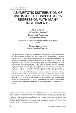
efficiency gain of the F̂n over Λ̂n by plotting (Var(F̂n )/Var(Λ̂n ))3/2 .
0.0
0.5
1.0
1.5
2.0
2.5
3.0
Time
Figure 1. The asymptotic relative efficiency of F̂n versus Λ̂n . N is the
number of simulation runs; n is the number of subjects.
278
SHUGUANG SONG
Random samples of univariate “mixed case” interval censored data Xi =
(i)
(i)
(∆Ki , TKi , Ki ), where i = 1, . . . , n, were generated as follows: Ki ∈ {1, 2, 3, 4, 5, 6,
(i)
7, 8} with P (Ki = k) = 1/8 for k = 1, . . . , 8; TKi are ordered sequence of Ki random variables generated from the unit exponential distribution; Each failure time
Y (i) was generated from the Weibull distribution with shape parameter equal to
(i)
2 and scale parameter equal to 2; the ∆Ki follow from ∆ki ,j = 1(T (i) ,T (i) ] (Y (i) )
for j = 1, . . . , ki + 1. The panel count data
(i)
(i)
(i)
(i)
(i)
(i)
(NKi , TKi , Ki )
ki ,j−1
ki ,j
: i = 1, . . . , n with
(i)
panel counts NKi = (NKi ,1 , NKi ,2 , . . . , NKi ,Ki ) are given by NKi ,j = 1[Y (i) ≤T (i)
Ki ,j ]
for j = 1, . . . , Ki . We ran Monte-Carlo simulations 1,000 times for the number
of subjects n = 100, and 200 times for n = 1, 000. The estimated efficiency gain
of F̂n over Λ̂n is plotted in Figure 1. As shown there, the NPMLE F̂n is more
efficient than the NPMLE Λ̂n : for most of the points where F̂n and Λ̂n were
estimated, the estimated asymptotic relative efficiency is above 40% for both
simulations. When time is between 0.2 and 1.6, the estimated asymptotic relative efficiency for the simulation with n = 100 is close to that for the simulation
with n = 1, 000; when the time varies from 1.8 to 3.0, the estimated asymptotic
relative efficiency for the simulation with n = 100 is generally higher than that
for the simulation case with n = 1, 000. Although Theorem 3.5 in Song (2001)
or Song (2002) and Theorem 4.4 in Wellner and Zhang (2000) show that the
asymptotic relative efficiency for the toy estimators of F̂n and Λ̂n is equal to
1 for a one jump process, the log-likelihood function for a one jump process in
Wellner and Zhang (2000) is different from that of (1.2).
5. Asymptotic Properties of the NPMLE: Proof
In this section, we give the proofs of the asymptotic properties of the NPMLE
in Section 3. More technical details can be found in Song (2001) and Song (2002).
Proof of Lemma 3.1. Construct the following brackets for the class M: mli ≡
2plF,i /(plF,i +pF0 )−1, and mri ≡ 2prF,i /(prF,i +pF0 )−1, where [plF,i , prF,i ], i = 1, . . . , I,
are brackets for class P. Since 1/(1 + t) is decreasing in t, and plF,i ≤ prF,i , so
for all mF ∈ M, there exists i ∈ {1, . . . , I} such that mlF,i ≤ mF ≤ mrF,i , and
|mri − mli |/2 = |prF,i (prF,i + pF0 ) − plF,i /(plF,i + pF0 )| = |pF0 (prF,i − plF,i )/[(prF,i +
pF0 )(plF,i + pF0 )]| ≤ 1. Thus, |mri − mli | ≤ 2 1[pF0 ≤σ] + 2 |mri − mli | 1[pF0 >σ] , and
mri −mli P,r ≡
|mri − mli |r dP
1/r
≤ (2r r + r )1/r , if (mri −mli )1pF0 >σ P,r ≤
. This implies that N[ ] ((2r + 1)1/r , M, Lr (P )) ≤ N[ ] (, Gσ0 , Lr (P )). Also,
dν, since pF0 /(plF,i +
(mri − mli ) 1[pF0 ≥σ] rP,r ≤ 2r |prF,i − plF,i |r 1[pF0 >σ] pF1−r
0
pF0 ) ≤ 1, and pF0 /(prF,i + pF0 ) ≤ 1. Define dQσ = (1[pF0 >σ] /pr−1
F0 )dν. Then
N[ ] (2, Gσ0 () , Lr (P )) ≤ N[ ] (, P, Lr (Qσ )).
ESTIMATION WITH UNIVARIATE “MIXED CASE” INTERVAL CENSORED DATA
279
Proof of Theorem 3.1. Define Jn ≡ [t0 − cn−1/3 , t0 + cn−1/3 ], and
Hn (t) ≡
θ f0 (t0 ) (t − t0 + cn−1/3 ), if t ∈ [t0 − cn−1/3 , t0 ),
θ f0 (t0 ) (t0 + cn−1/3 − t), if t ∈ [t0 , t0 + cn−1/3 ],
0,
otherwise.
Note that pFn (δ, t) = pF0 (δ, t) + (θ f0 (t0 )) k+1
j=1 δk,j (Hn (tk,j ) − Hn (tk,j−1 )), and
−1/3
|Fn (t0 ) − F0 (t0 )| = θ f0 (t0 ) c n
. Under the separation condition B, and
for large n, tk,j and tk,j−1 will not be in Jn at the same time. This indicates that |Hn (tk,j ) − Hn (tk,j−1 )| = Hn (tk,j ) or Hn (tk,j−1 ) ≤ θ f0 (t0 ) c n−1/3 .
√
√
Thus [1/( pFn + pF0 )]2 = 1/(4 pF0 ) + O(n−1/3 ) 1Jn (t), and (pFn − pF0 )2 dν =
∞
k+1 2
2
k=1 P (K = k)
j=1 (Hn (tk,j ) − Hn (tk,j−1 )) dQ(tk |K = k) = (2/3)(θf0 (t0 ))
k+1
∞
−1
−1
c3 n−1 ( ∞
k=1 P (K = k)
k=1
j=1 (qk,j (t0 ) + qk,j−1(t0 ))) + o(n ) = O(n ), if
k+1
P (K = k) j=1 (qk,j (t0 ) + qk,j−1(t0 )) < ∞. The above condition is satisfied if
EK < ∞ and qk,j is bounded above for all j = 1, . . . , k, k = 1, . . .. The Hellinger
distance becomes h2 (pFn , pF0 ) = (1/8) [(pFn − pF0 )2 /pF0 ]dν + o(n−1 ). Now,
∞
k+1
(pFn − pF0 )2
dν =
P (K = k)
pF 0
j=1
k=1
(Hn (tk,j ) − Hn (tk,j−1 ))2
dQ(tk |K = k)
F0 (tk,j ) − F0 (tk,j−1 )
= 2 a(t0 ) (θf0 (t0 ))2 c3 n−1 + o(n−1 ).
Thus, h2 (pFn , pF0 ) = (1/4) a(t0 ) (θf0 (t0 ))2 c3 n−1 + o(n−1 ).
By (3.1), we have n1/3 inf Tn max{En, pFn | Tn − Fn (t0 )|, En, pF0 | Tn −
F0 (t0 )|} ≥ 0.25n1/3 |Fn (t0 ) − F0 (t0 )|{1 − h2 (pFn , pF0 )}2n ≥ 0.25θcf0 (t0 )(1 −
2 3
0.25a(t0 )(θf0 (t0 ))2 c3 n−1 + o(n−1 ))2n → 0.25θcf0 (t0 )e−a(t0 )(θf0 (t0 )) c /2 . The last
expression is maximized by c ≡ {1.5a(t0 )θ 2 f02 (t0 )}−1/3 , and the maximum value
is 0.25 (2θ/3)1/3 e−1/3 (f0 (t0 )/a(t0 ))1/3 . Thus,
lim inf n
n→∞
1/3
max {En,pFn |Tn − Fn (t0 )|, En,pF0 |Tn − F0 (t0 )|} ≥ c0
f0 (t0 )
a(t0 )
1/3
,
where c0 ≡ 0.25 (2θ/3)1/3 e−1/3 is a constant depending on θ.
Proof of Lemma 3.2. By Theorem 2.7.5 in Van der Vaart and Wellner (1996),
for all > 0 and for any probability measure Q, there exists a constant L such
that log N[ ] (, F, L2 (Q)) ≤ L (1/). This implies that for all F ∈ F, there
exists a bracket [Fil (t), Fir (t)] such that Fil (t) ≤ F (t) ≤ Fir (t) for all t and some
i ∈ {1, . . . , I}, and Fir (tK,j ) − Fil (tK,j )
PK,j ,2 ≤ for j = 1, . . . , K, K = 1, 2, . . ..
Then we have Fil (tK,j )−Fir (tK,j−1 ) ≤ F (tK,j )−F (tK,j−1 ) ≤ Fir (tK,j )−Fil (tK,j−1 ).
Note that mF = 2 K+1
j=1 δK,j [F (TK,j )−F (TK,j−1 )]/[(F (TK,j )−F (TK,j−1 ))+
(F0 (TK,j ) − F0 (TK,j−1 ))] − 1 ≡ 2 K+1
j=1 δK,j ∆FK,j /(∆FK,j + ∆F0,K,j ) − 1. Also,
280
SHUGUANG SONG
+ a)) = a/(x + a)2 > 0 for a > 0 and, under conditions B and C,
there exists a η > 0 such that F0 (TK,j ) − F0 (TK,j−1 ) > η for all j = 1, . . . , K,
K = 1, 2, . . .. Thus, 0 < ∆F0,K,j ≤ 1, and ∆FK,j /(∆FK,j + ∆F0,K,j ) is increasing
in ∆FK,j ≥ 0. Choose the brackets of M as
d
dx (x/(x
mli (X) = 2
K+1
δK,j Fil (TK,j ) − Fir (TK,j−1 )
− 1,
Fil (TK,j ) − Fir (TK,j−1 ) + ∆F0,K,j
δK,j Fir (TK,j ) − Fil (TK,j−1 )
r
Fi (TK,j ) − Fil (TK,j−1 ) + ∆F0,K,j
j=1
mri (X) = 2
K+1
j=1
− 1,
where i = 1, . . . , I. Then, it follows that 0.25P (|mri − mli |2 ) = ∞
k=1 P (K =
k+1 r
l
r
l
k) j=1 {(Fi (tk,j ) − Fi (tk,j−1 ))/[(Fi (tk,j ) − Fi (tk,j−1 )) + ∆F0,k,j ] − (Fil (TK,j ) −
Fir (TK,j−1 ))/[Fil (TK,j )−Fir (TK,j−1 )+∆F0,K,j ]}2 ∆F0,k,j dQ(tk |K = k) 42 (EK
+1) < ∞, if EK < ∞. Here, symbol denotes that the left term is less than the
right term up to a constant. This implies that log N[ ] (, M, L2 (P )) = O(1/).
Proof of Theorem 3.2. In order to apply Corollary 3.2.6 in Van der Vaart and
Wellner (1996), we need to use Lemma 3.4.2 in Van der Vaart and Wellner (1996)
to find an upper bound√for E ∗ Gn Mδ ,√where Mδ ≡ {mF : h(pF , pF0 ) < δ}. For
mF ∈ Mδ , P (m2F ) ≤ 2h(pF , pF0 ) < 2 δ. Also, for all mF ∈ Mδ , m2F ∞ ≤
1. Thus, by Lemma 3.4.2 in Van der Vaart and Wellner (1996), E ∗ Gn Mδ ≤
√
J˜[ ] (δ, Mδ , L2 (P )) (1 + J˜[ ] (δ, Mδ , L2 (P ))/(δ2 n)), where J˜[ ] (δ, Mδ , L2 (P )) ≡
δ
+ log N[ ] (, Mδ , L2 (P ))}1/2 d ≤ oδ {1 + log N[ ] (, MF , L2 (P ))}1/2 d =
+ O(1/)}1/2 d = O(δ1/2 ). Then it follows from Corollary 3.2.6 in Van
√
der Vaart and Wellner (1996) that E ∗ Gn Mδ δ1/2 (1 + δ1/2 /(δ2 n)) =
√
√
√
−1/2
+ rn / n) ≤ n, we
δ1/2 + 1/(δ n) ≡ φ(δ). From rn2 · φ(1/rn ) = rn2 (rn
have rn ≤ n1/3 . Thus the rate is n1/3 .
{1
0δ
0 {1
Proof of Theorem 3.3. We use Lemma 3.1 to control the bracketing entropy of the class M. In this case, r = 2, so dQσ = (1[pF0 > σ] /pF0 ) dν. Let
l
[pli , pri ] be a pair of bracket for the class P as defined as plF,i ≡ ΠK+1
j=1 (Fi (tK,j ) −
r
l
δK,j . Note that pr −pl 2
Fir (tK,j−1))δK,j , prF,i ≡ ΠK+1
i
i Qσ ,2 =
j=1 (Fi (tK,j )−Fi (tK,j−1))
r
−1
l
2
r
l
2
(F (tk,j )−Fi (tk,j )) 1[pF0 > σ] pF0 dν + (Fi (tk,j−1 )−Fi (tk,j−1 )) 1[pF0 > σ] p−1
F0 dν +
i r
−1
l
r
l
2(Fi (tk,j )−Fi (tk,j )) (Fi (tk,j−1 )−Fi (tk,j−1 )) 1[pF0 > σ] pF0 dν. Define dQ̄(tk |K =
k) = (1[pF0 > σ] / (pF0 (1[pF0 > σ] /pF0 ) dν))dν. Then (Fir (tk,j )−Fil (tk,j ))2 dQ̄(tk |K
= k) ≤ 2 , and (Fir (tk,j−1 ) − Fil (tk,j−1 ))2 dQ̄(tk |K = k) ≤ 2 . By the Cauchy
Schwarz inequality, (Fir (tk,j )−Fil (tk,j )) (Fir (tk,j−1 )−Fil (tk,j−1 )) dQ̄(tk |K = k) ≤
{ (Fir (tk,j ) − Fil (tk,j ))2 dQ̄(tk |K = k) · (Fir (tk,j−1 ) − Fil (tk,j−1 ))2 dQ̄(tk | K =
k)}1/2 ≤ · = 2 . Thus, we have pri − pli Qσ ,2 ≤ 2 { (1[pF0 > σ] /pF0 ) dν}1/2 =
ESTIMATION WITH UNIVARIATE “MIXED CASE” INTERVAL CENSORED DATA
281
2 { dQσ }1/2 . This shows log N[ ] (, P, L2 (Qσ )) = O({ dQσ }1/2 /). Now for
fixed k ≥ 1 and 1 ≤ j ≤ k, 1[F0 (tk,j )−F0 (tk,j−1 )>σ] /[F0 (tk,j )−F0 (tk,j−1 )]dQ(tk |K =
k) = 1[F0 (tk,j )−F0 (tk,j−1 )>σ] qk,j,j−1f0 (tk,j )f0 (tk,j−1 )/[(F0 (tk,j )−F0 (tk,j−1 ))f0 (tk,j )
f0 (tk,j−1 )]dtk,j dtk,j−1 ≤ c0 c1 log(c1 /σ), where c0 , c do not depend on j and k by
k
assumption D. Hence we have dQσ ≤ ∞
k=1 P (K = k)
j=1 c0 c1 log(c1 /σ) =
c0 c1 (EK) log(c1 /σ).
Recall that we require pF ≤ σ pF0 dν ≤ 2 , and pF ≤ σ pF0 dνσ(EK). Take
0
0
σ = 2 /EK. Then, if EK < ∞, log N[ ] (, P, L2 (Qσ )) (1/) log1/2 (1/). By
Lemma 3.1, log N[ ] (, Mδ , L2 (P )) (1/) log1/2 (1/). We have shown that
√
2
mF 1[h(pF ,pF0 ) < δ] dP < 2 δ. It follows that
J˜[ ] (δ, Mδ , L2 (P )) =
δ
0
δ
o
δ 1/2
1 + log N[ ] (, Mδ , L2 (P )) d
1
1
log1/2 ( ) d
1
log1/4 .
δ
By Lemma 3.4.2 in Van der Vaart and Wellner (1996), E ∗ Gn Mδ δ1/2 log1/4
√
√
(1/δ) (1 + (δ1/2 log1/4 (1/δ))/( n δ2 )) = δ1/2 log1/4 (1/δ) + log1/2 (1/δ)/( n δ) ≡
φ(δ). By Corollary 3.2.6 in Van der Vaart and Wellner (1996), we have rn2 φ(1/rn )
√
√
√
−1/2
log1/4 rn + (rn log rn )/ n) ≤ n. This yields rn ≤ n1/3 log−1/6 n.
= rn2 (rn
Thus the rate is n1/3 log−1/6 n.
Acknowledgements
This paper is part of author’s Ph.D. dissertation under supervision of Professor Jon A. Wellner. Some writing and computation was carried out while the
author was employed by the Boeing Company. The author thanks an editor, an
associate editor and an anonymous referee for their valuable suggestions. This
research was partially supported by National Science Foundation grant DMS9971951.
References
Aragón, J. and Eberly, D. (1992). On convergence of convex minorant algorithm for distribution
estimation with interval-censored data. J. Comput. Graph. Statist. 1, 129-140.
Becker, N. G. and Melbye, M. (1991). Use of log-linear model to compute the empirical survival
curve from interval-censored failure time data, with application to data on tests for HIV
positivity. Austral. J. Statist. 33, 125-133.
Finkelstein, D. M. (1986). A proportional hazards model for interval-censored failure time data.
Biometrics 42, 845-854.
282
SHUGUANG SONG
Finkelstein, D. M. and Wolfe, R. A. (1985). A semiparametric model for regression analysis of
interval-censored failure time data. Biometrics 41, 993-945.
Groeneboom, P. (1991). Nonparametric maximum likelihood estimators for interval censoring
and deconvolution. Technical Report 378, Department of Statistics, Stanford University.
Groeneboom, P. (1996). Lectures on inverse problems. In Lectures on Probability Theory and
Statistics 1648, Lectures Notes in Mathematics (Edited by P. Bernard), 67-136. SpringerVerlag, Berlin.
Groeneboom, P. and Wellner, J. A. (1992). Information Bounds and Nonparametric Maximum
Likelihood Estimation, DMV Seminar Band 19, Birkhäuser, Basel.
Groeneboom, P. and Wellner, J. A. (2001). Computing Chernoff’s distribution. J. Comput.
Graph. Statist. 10, 388-400.
Huang, J. and Wellner, J. A. (1997) Interval censored survival data: a review of recent progress.
In Proceedings of the First Seattle Symposium in Biostatistics: Survival Analysis 123,
Lecture Notes in Statistics (Edited by D. Y. Lin and Thomas. R. Fleming), 123-169.
Springer Verlag, Berlin.
Jongbloed, G. (1995). Three statistical inverse problems. Ph.D. thesis, Delft Technological
University, The Netherlands.
Jongbloed, G. (1998). The iterative convex minorant algorithm for nonparametric estimation.
J. Comput. Graph. Statist. 7, 310-321.
Schick, A. and Yu, Q. (2000). Consistency of the GMLE with mixed case interval censored
data. Scand. J. Statist. 27, 45-55.
Self, S. G. and Grossman, E. A. (1986). Linear rank tests for interval-censored data with
application to PCB levels in adipose tissue of transformer repair workers. Biometrics 42,
521-530.
Song, S. (2001). Estimation with bivariate interval censored data. Ph. D. thesis, University of
Washington.
Song, S. (2002). Estimation with univariate “mixed case” interval censored data. Technical
Report 414, Department of Statistics, University of Washington.
Turnbull, B. W. (1976). The empirical distribution function with arbitrary grouped, censored
and truncated data. J. Roy. Statist. Soc. Ser. B 38, 290-295.
Van der Vaart, A. W. and Wellner, J. A. (1996). Weak Convergence and Empirical processes
with Application to Statistics. Springer, New York.
Van der Vaart, A. W. and Wellner, J. A. (2000). Preservation theorems for Glivenko-Cantelli
and uniform Glivenko-Cantelli classes. In High Dimensional Probability II (Edited by E.
Giné, D. M. Mason and J. A. Wellner), 115-133. Birkhäuser, Basel.
Wellner, J. A. (1995). Interval censoring case 2: alternative hypotheses. In Analysis of Censored Data 27, IMS Lecture Notes - Monograph Series (Edited by H. L. Koul and J. V.
Deshpande), 271-291. IMS, Hayward.
Wellner, J. A. and Zhan, Y. (1997). A hybrid algorithm for computation of the nonparametric
maximum likelihood estimator from censored data. J. Amer. Statist. Assoc. 92, 272–291.
Wellner, J. A. and Zhang, Y. (2000). Two estimators of the mean of a counting processes with
panel count data. Ann. Statist. 28, 779-814.
Applied Statistics, Phantom Works, The Boeing Company, P.O. Box 3707, MS 7L-22, Seattle,
Washington 98124-2207, U.S.A.
E-mail: [email protected]
(Received October 2002; accepted March 2003)
© Copyright 2026 Paperzz