MEASURE THEORY
ARIEL YADIN
Course: 201.1.0081
Fall 2014-15
Lecture notes updated: January 22, 2015
(partial solutions)
Contents
Lecture 1.
4
Introduction
1.1.
Measuring things
4
1.2.
Elementary measure
5
This lecture has 6 exercises.
Lecture 2.
2.1.
11
12
Jordan measure
Jordan measure
12
This lecture has 15 exercises.
Lecture 3.
3.1.
24
25
Lebesgue outer measure
From finite to countable
25
This lecture has 5 exercises.
Lecture 4.
29
30
Lebesgue measure
4.1.
Definition of Lebesgue measure
30
4.2.
Lebesgue measure as a measure
37
This lecture has 12 exercises.
Lecture 5.
43
44
Abstract measures
5.1. σ-algebras
44
5.2.
Measures
47
5.3.
Fatou’s Lemma and continuity
50
This lecture has 13 exercises.
Lecture 6.
52
53
Outer measures
1
2
6.1.
Outer measures
53
6.2.
Measurability
54
6.3.
Pre-measures
57
This lecture has 12 exercises.
Lecture 7.
Lebesgue-Stieltjes Theory
62
63
7.1.
Lebesgue-Stieltjes measure
63
7.2.
Regularity
68
7.3.
Non-measureable sets
69
7.4.
Cantor set
69
This lecture has 6 exercises.
Lecture 8.
Functions of measure spaces
70
71
8.1.
Products
71
8.2.
Measurable functions
73
8.3.
Simple functions
78
This lecture has 20 exercises.
80
Lecture 9.
Integration: positive functions
81
9.1.
Integration of simple functions
81
9.2.
Integration of positive functions
83
This lecture has 7 exercises.
Lecture 10.
Integration: general functions
89
90
10.1.
Real valued functions
90
10.2.
Complex valued functions
91
10.3.
Convergence
93
10.4.
Riemann vs. Lebesgue integration
97
This lecture has 10 exercises.
Lecture 11.
Product measures
101
102
11.1.
Sections
105
11.2.
Product integrals
107
3
11.3.
The Fubini-Tonelli Theorem
This lecture has 19 exercises.
Lecture 12.
Change of variables
114
120
121
12.1.
Linear transformations of Lebesgue measure
121
12.2.
Change of variables formula
124
This lecture has 4 exercises.
Lecture 13.
Lebesgue-Radon-Nykodim
128
129
13.1.
Signed measures
129
13.2.
The Lebesgue-Radon-Nikodym Theorem
136
This lecture has 27 exercises.
Lecture 14.
146
Convergence
147
14.1.
Modes of convergence
147
14.2.
Uniform and almost uniform convergence
153
This lecture has 10 exercises.
Lecture 15.
Differentiation
157
158
15.1.
Hardy-Littlewood Maximal Theorem
158
15.2.
The Lebesgue Differentiation Theorem
161
15.3.
Differentiation and Radon-Nykodim derivative
162
This lecture has 6 exercises.
Lecture 16.
The Riesz Representation Theorem
164
165
16.1.
Compactly supported functions
165
16.2.
Linear functionals
168
16.3.
The Riesz Representation Theorem
169
This lecture has 5 exercises.
174
Total number of exercises: 177
174
4
Measure Theory
Ariel Yadin
Lecture 1: Introduction
1.1. Measuring things
Already the ancient Greeks developed a theory of how to measure length, area, and
volume and area of 1, 2 and 3 dimensional objects. In this setting (i.e. in Rd for d ≤ 3)
it stands to reason that the “size” or “measure” of an object must satisfy some basic
axioms:
• If m(A) is the measure of a set A, it should be the same for any reflection,
translation or rotation of A. That is, m(A) = m(A + x) = m(U A) where U is a
rotation matrix.
For example, [0, 1]2 should heave the same measure as [−2, −1]2 which should
o
n
have the same measure as (x, y) : |x| + |y| ≤ √12 , the diamond of side-length
1.
• If A can be broken into disjoint pieces, the sum of their measures should be the
measure of A. That is, m(A ] B) = m(A) + m(B).
Example: [0, 1] × [0, 2] should have measure that is the sum of the measures
of [0, 1]2 and [0, 1] × (1, 2].
X We use ] to denote disjoint union; that is, A ] B is not only notation for a set,
but this notation claims that A ∩ B = ∅. The small + sign remind us of the additive
property above.
This is already quite fruitful. If the unit square (0, 1]2 is of measure 1, then:
• We can determine the measure of any square of rational side length.
m((0, n]2 ) =
n
X
j,k=1
m((j − 1, j] × (k − 1, k]) = n2
5
and
m((0, 1]2 ) =
n
X
j,k=1
j
2
k−1 k
1 2
m(( j−1
n , n ] × ( n , n ]) = n m((0, n ] ).
• We can measure any rectangle of rational side length: decompose it into squares.
• We can measure right-angle triangles: disjoint union of two is a rectangle.
• We can then measure any triangle, by bounding it in a rectangle and subtracting
the excess right-angle triangles.
• With triangles we can measure any polygon.
X What about measuring a disc?
1.2. Elementary measure
Let us first formally define the above.
• Definition 1.1 (Boxes). Consider Rd for some d ≥ 1.
• I ⊂ R is an interval if I is one of [a, b], (a, b), (a, b], [a, b) for some −∞ < a ≤ b <
∞. Note that we allow the singleton {a} = [a, a] as an interval, and the empty set
∅ = (a, a). The length or measure of such I is defined to be |I| = m(I) = b−a.
• B ⊂ Rd is a box if B = I1 × · · · × Id where Ij are intervals. The volume or
measure of such a box B is defined to be |B| = m(B) = |I1 | · · · |Id |.
• E ⊂ Rd is an elementary set if E = B1 ∪ · · · ∪ Bn for some finite number of
boxes.
• E0 = E0 (Rd ) denotes the set of elementary sets in Rd .
Exercise 1.1.
Show that E0 is closed under finite unions, finite intersections,
set-difference, symmetric difference and translations. That is, show that if E, F are
elementary sets then so are:
• E ∪ F and E ∩ F ,
• E \ F := {x ∈ E : x 6∈ F } = E ∩ F c ,
• E4F := (E \ F ) ∪ (F \ E),
6
• E + x := {y + x : y ∈ E}.
Exercise 1.2.
Show that if E is an elementary set then there exist B1 , . . . , Bn
pairwise disjoint boxes such that E = B1 ] · · · ] Bn .
It would be tempting to define the measure of E = B1 ]· · ·]Bn as m(B1 )+· · ·+m(Bn ).
But we are not guarantied that the decomposition is a unique one.
• Proposition 1.2 (Discretisation Formula). Let I be an interval. Then,
1
#(I ∩ n1 Z).
n→∞ n
m(I) = lim
Consequently, if B ⊂ Rd is a box then,
1
#(B ∩ n1 Zd ),
n→∞ nd
m(B) = lim
and if E = B1 ] · · · ] Bn ⊂ Rd is an elementary set then
m(B1 ) + · · · + m(Bn ) = lim
n→∞
1
#(E ∩ n1 Zd ).
nd
Proof. Let a < b and I be an interval with endpoints a, b. For n large enough, note that
#(I ∩ n1 Z) = # z ∈ Z :
z
n
∈ I ≤ # {z ∈ Z : na ≤ z ≤ nb}
≤ # {z ∈ Z : bnac ≤ z ≤ dnbe} ≤ nb + 1 − (na − 1) + 1 = n(b − a) + 3.
Similarly,
#(I ∩ n1 Z) ≥ # {z ∈ Z : na < z < nb} ≥ n(b − a) − 1.
Dividing by n and taking n → ∞ we obtain the formula for intervals.
Now, if B = I1 × · · · × Id then
B ∩ n1 Zd = (I1 ∩ n1 Z) × · · · × (Id ∩ n1 Z),
7
which implies that
#(B ∩ n1 Zd ) =
d
Y
j=1
#(Ij ∩ n1 Z).
Dividing by nd and taking n → ∞ gives the formula for boxes.
The final assertion is a consequence of the fact that if A ∩ B = ∅ then
(A ] B) ∩ n1 Zd = (A ∩ n1 Zd ) ] (B ∩ n1 Zd ).
t
u
• Definition 1.3. If E = B1 ] · · · ] Bn is an elementary set we define the measure of
E to be
1
#(E ∩ n1 Z),
n→∞ nd
m(E) = m(B1 ) + · · · + m(Bn ) = lim
which is well defined by Proposition ??.
Exercise 1.3. Give an example of a set A ⊂ [0, 1] such that the limit
1
#(A ∩ n1 Z)
n→∞ n
lim
does not exist.
1
#(A ∩ n1 Z)
n→∞ n
both exist but are not equal.
lim
♣ Solution to ex:1.3.
and
1
#((A + x) ∩ n1 Z)
n→∞ n
lim
:(
For the first example: Set
A=
2m−1
2n
: Z 3 n, m ≥ 1 , 2m − 1 ≤ 2n .
Since for any z ≥ 1 we can write z = (2m − 1)2k for some k ≥ 0 and m ≥ 1, we have
that
#(A ∩ 2−n Z) ≥ #
z
2n
: 1 ≤ z ≤ 2n = 2n .
8
So
lim sup n1 #(A ∩ n1 Z) ≥ lim sup 2−n #(A ∩ 2−n Z) = 1.
n→∞
n→∞
On the other hand, if x ∈ A ∩ 3−k Z then for some m, n ≥ 1 and z ∈ Z, x =
2m−1
2n
=
z
3k
which implies that 2n z = 3k (2m − 1). The left hand side is even while the right hand
side is odd, which is a contradiction. So A ∩ 3−k Z = ∅ for all k, and we conclude that
lim inf n1 #(A ∩ n1 Z) ≤ lim inf 3−n #(A ∩ 3−n Z) = 0.
n→∞
n→∞
For the second example take A = Q ∩ [0, 1] and x = π.
:) X
This last exercise shows that we do not want to use the discretization formula to
define the measure of general sets, but we can use it for more than just elementary sets.
Exercise 1.4. Show that the measure of elementary sets has the following prop-
erties.
• m : E0 → [0, ∞).
• (Additivity) m(E ] F ) = m(E) + m(F ).
• m(∅) = 0.
• If B is a box, then m(B) = |B|.
• (Monotonicity) If E ⊂ F then m(E) ≤ m(F ).
• (Subadditivity) m(E ∪ F ) ≤ m(E) + m(F ).
• (Translation invariance) For any x ∈ Rd , m(E + x) = m(E).
♣ Solution to ex:1.4.
:(
The discretization formula guaranties that m is non-negative and additive, m(∅) = 0
and also that if B is a box then m(B) = |B|.
For monotonicity recall that F \ E is elementary, and F = (F ∩ E) ] (F \ E). Since
E ⊂ F we have that F ∩ E = E. So m(F ) = m(E) + m(F \ E) ≥ m(E).
Subadditivity follows from E ∪ F = E ] (F \ E) so
m(E ∪ F ) = m(E) + m(F \ E) ≤ m(E) + m(F ).
9
Translation invariance is another consequence of the discretization formula: For any
z
n
interval I with endpoints a < b, we have that
if
z
n
− x ∈ I if and only if z ∈ nI + nx. Thus,
− x ∈ I then z ∈ [bna + nxc, dnb + nxe] ∩ Z and if z ∈ [dna + nxe, bnb + nxc] ∩ Z
then
z
n
− x ∈ I. Since
#([bna+nxc, dnb+nxe]∩Z) ≤ n(b−a)+3
#([dna+nxe, bnb+nxc]∩Z) ≥ n(b−a)−1,
and
we have
z
n
# z ∈ Z :
− x ∈ I − n(b − a) ≤ 3.
Dividing by n and taking a limit we get that
1
#
n→∞ n
m(I + x) = lim
z∈Z :
z
n
− x ∈ I = b − a = m(I).
If B = I1 ×· · ·×Id is a box in Rd , then for any x ∈ Rd , B+x = (I1 +x1 )×· · ·×(Id +xd ),
Q
Q
so m(B + x) = dj=1 m(Ij + xj ) = dj=1 m(I) = m(B).
Finally, if E = B1 ]· · ·]Bk is an elementary set, then E +x = (B1 +x)]· · ·](Bk +x).
So m(E + x) = m(E).
:) X
Exercise 1.5. Show that if m0 : E0 → [0, ∞) is additive and translation invariant,
i.e. m(E ] F ) = m(E) + m(F ) and m(E + x) = m(E), then there exists a constant c ≥ 0
such that m0 = cm.
♣ Solution to ex:1.5.
:(
If E = B1 ] · · · ] Bk is an elementary set then m0 (E) = m0 (B1 ) + · · · + m0 (Bk ). So we
only need to show that m0 (B) = c|B| for any box B.
First, note that since
[0, 1) =
n
]
j=1
1
n [j
− 1, j)
and
[0, nk ) =
n
]
j=1
1
k [j
− 1, j),
additivity and translation invariance guaranty that
m0 ([0, n1 )d ) =
1
m0 ([0, 1)d )
nd
and
m0 ([0, q)d ) = q d · m0 ([0, 1))
10
for any q ∈ Q (make sure to fill in the details here). By translation invariance, for any
aj ≤ bj ∈ Q we then have
m0 ([a1 , b1 ) × · · · × [ad , bd )) =
d
Y
(bj − aj ) · m0 ([0, 1)d ).
j=1
Set C = m0 ([0, 1)d ).
Let B = I1 × · · · × Id . Assume that the endpoints of Ij are aj < bj .
+ − +
Fix ε > 0 such that for all j we have bj − aj > 2ε. Let a−
j , aj , bj , bj be rational
−
+
−
numbers such that a+
j ∈ (aj , aj + ε), aj ∈ (aj − ε, aj ), bj ∈ (bj , bj + ε), bj ∈ (bj − ε, bj ).
+
−
+ −
± = I ± × · · · × I ± , so B − ⊂ B ⊂ B + .
Let Ij+ = [a−
1
j , bj ) and Ij = [aj , bj ). Let B
d
Since m0 is additive and non-negative, it is also monotone. Monotonicity tells us that
m0 (B − ) ≤ m0 (B) ≤ m0 (B + ).
±
Because a±
j , bj ∈ Q we get that
m0 (B + ) =
d
Y
−
(b+
j − aj ) · C ≤
j=1
0
−
m (B ) =
d
Y
(b−
j
j=1
−
a+
j )
·C ≥
d
Y
(bj − aj + 2ε) · C,
j=1
d
Y
(bj − aj − 2ε) · C.
j=1
Setting M = maxj (bj − aj ) we have that
m0 (B + ) −
d
Y
d
Y
(bj − aj ) · C ≤ C · 2ε · dM d−1 ,
j−1
(bj − aj ) · C − m0 (B − ) ≤ C · 2ε · dM d−1 .
j−1
Taking ε → 0 we get that
m0 (B) =
d
Y
(bj − aj ) · C = m0 ([0, 1)d ) · m(B).
j=1
:) X
Exercise 1.6.
Let E ⊂ Rd and F ⊂ Rk be elementary sets. Show that E × F is
elementary (in Rd+k ) and that m(E × F ) = m(E) · m(F ).
11
Number of exercises in lecture: 6
Total number of exercises until here: 6
12
Measure Theory
Ariel Yadin
Lecture 2: Jordan measure
2.1. Jordan measure
We have seen that the measure of elementary sets is a good way to measure length,
area and volume for squares and rectangles, and anything that can be composed of
finite unions of such. How about measuring a triangle? Or a circle? We saw that the
discretisation formula also has its limitations. However, Jordan measure is essentially
the way to use the discretisation formula.
Jordan measure is essentially approximating general shapes by elementary ones.
• Definition 2.1 (Jordan measure). Let A ⊂ Rd be a bounded set (i.e. A ⊂ B(0, r) :=
{x : |x| ≤ r}). Define:
• The Jordan inner measure of A
J∗ (A) :=
sup m(A).
E0 3E⊂A
• The Jordan outer measure of A
J ∗ (A) :=
inf
E0 3F ⊃A
m(F ).
• If A is such that J∗ (A) = J ∗ (A) we say that A is Jordan measurable. We then
define the Jordan measure of A as this common value, m(A) = J∗ (A) = J ∗ (A).
Exercise 2.1. Show that J ∗ , J∗ are monotone. Show that J ∗ is subadditive.
♣ Solution to ex:2.1.
:(
Let A ⊂ C. Let (En )n , (Fn )n be sequences of elementary sets such that En ⊂ A, C ⊂ Fn
13
and m(En ) → J∗ (A), m(Fn ) → J ∗ (C). Note that for every n,
J∗ (C) ≥ m(En ) → J∗ (A)
and
J ∗ (A) ≤ m(Fn ) → J ∗ (C).
Also, if (Gn )n is a sequence of elementary sets such that A ⊂ Gn and m(Gn ) → J ∗ (A),
then A ∪ C ⊂ Gn ∪ Fn so
J ∗ (A ∪ C) ≤ m(Gn ∪ Fn ) ≤ m(Gn ) + m(Fn ) → J ∗ (A) + J ∗ (C).
:) X
Note that every elementary set E is Jordan measurable and m(E) = J ∗ (E) = J∗ (E).
Jordan sets are those which are “almost elementary”.
Exercise 2.2. Show that the following are equivalent for bounded A ⊂ Rd .
• A is Jordan measurable.
• For every ε > 0 there exist elementary sets E ⊂ A ⊂ F , E, F ∈ E0 , such that
m(F \ E) < ε.
• For every ε > 0 there exists an elementary set E0 3 E ⊂ A such that J ∗ (A\E) <
ε.
♣ Solution to ex:2.2.
:(
For any ε > 0 there exist elementary sets E ⊂ A ⊂ F such that m(E) > J∗ (A) − ε and
m(F ) < J ∗ (A) + ε. So if A is Jordan measurable then m(F ) < J ∗ (A) + ε = J∗ (A) + ε <
m(E) + 2ε. Since E ⊂ F we have that m(F ) = m(E) + m(F \ E), so m(F \ E) < 2ε.
Now assume that there exist E, F ∈ E0 , E ⊂ A ⊂ F such that m(F \ E) < ε. Then,
A \ E ⊂ F \ E, so J ∗ (A \ E) ≤ m(F \ E) < ε.
Finally assume that for every ε > 0 there exists an elementary set Eε ⊂ A such that
J ∗ (A
\ Eε ) < ε. Since Eε ⊂ A we have that m(Eε ) ≤ J∗ (A). Using the subadditivity of
J ∗ we get
J ∗ (A) ≤ J ∗ (A \ Eε ) + m(Eε ) < ε + J∗ (A).
14
Taking ε → 0 and recalling that J∗ (A) ≤ J ∗ (A) by definition, we have that J ∗ (A) =
J∗ (A) and aso A is jordan measurable.
:) X
Exercise 2.3. Show that for Jordan measurable sets A, C the following holds.
• A ∪ C, A ∩ C, A \ C, A4C are all Jordan measurable.
• m(A) ≥ 0.
• (Additivity) If A ∩ C = ∅ then m(A ] C) = m(A) + m(C).
• (Monotonicity) If C ⊂ A then m(C) ≤ m(A).
• (Subadditivity) m(A ∪ C) ≤ m(A) + m(C).
• (Translation invariance) m(A + x) = m(A).
Exercise 2.4. Show that a bounded set A is Jordan measurable if and only if for
every ε > 0 there exists an elementary set E such that A ⊂ E and J ∗ (E \ A) < ε.
♣ Solution to ex:2.4.
:(
Let B be a box containing the bounded set A.
Suppose that there exists an elementary set F ⊂ B \ A such that J ∗ ((B \ A) \ F ) < ε.
Then, with E = B \ F we have that A ⊂ E and J ∗ (E \ A) = J ∗ ((B \ A) \ F ) < ε.
Thus we obtain that A is Jordan measurable iff B \ A is Jordan measurable iff for
every ε > 0 there exists an elementary set F , F ⊂ B \ A, such that J ∗ ((B \ A) \ F ) < ε
iff for every ε > 0 there exists an elementary set E, A ⊂ E, such that J ∗ (E \ A) < ε. :)
X
Exercise 2.5. [Tao, ex. 1.1.7] Let B ⊂ Rd be a closed box, and let f : B → R be a
continuous function. Show that
• The graph {(x, f (x)) : x ∈ B} is Jordan measurable with Jordan measure 0.
15
• The volume under the graph {(x, t) : x ∈ B, 0 ≤ t ≤ f (x)} is Jordan measurable.
♣ Solution to ex:2.5.
:(
f is uniformly continuous in B; that is, for every ε > 0 there exists δ > 0 such that for
any ||x − y|| < δ we have |f (x) − f (y)| < ε.
S
Write B = N
n=1 Bδ (xn ) where (Bδ (xn ))n are disjoint boxes of diameter less than δ,
with xn the center of Bδ . Uniform continuity of f gives that for any x ∈ B there exists (a
unique) n such that x ∈ Bδ (xn ), and so (x, f (x)) ∈ Bδ (xn )×(f (xn )−ε, f (xn )+ε) =: Qδ,n .
S
Thus, {(x, f (x)) : x ∈ B} ⊂ Qδ,n . Since m(Qδ,n ) = m(Bδ (xn )) · 2ε, we have that
J ∗ ({(x, f (x)) : x ∈ B}) ≤
X
n
m(Qδ,n ) ≤ 2ε
X
m(Bδ (xn )) = 2εm(B).
n
Taking ε → 0 gives the first assertion.
For the second assertion, let V = {(x, t) : x ∈ B, 0 ≤ t ≤ f (x)}. Fix ε, δ > 0 and
S
B = n Bδ (x) as above. For every n set
mn =
inf
x∈Bδ (xn )
f (x)
Mn =
sup
f (x).
x∈Bδ (xn )
Note that |Mn − mn | ≤ ε by uniform continuity. Now, set Kn = b mεn c. For 0 ≤ k ≤
Kn − 1 set Qn,k = Bδ (xn ) × ε[k, k + 1) and Q̃n = Bδ (xn ) × [εKn , Mn ].
For any n, if 0 ≤ k < Kn and (x, t) ∈ Qn,k then x ∈ Bδ (xn ) and t < εKn ≤ mn ≤ f (x).
So
n −1
[ K[
n
k=0
Qn,k ⊂ V.
On the other hand, if x ∈ B and 0 ≤ t ≤ f (x) then there exists n such that x ∈ Bδ (xn )
and so f (x) ∈ [mn , Mn ]. Thus, either t < εKn in which case (x, t) ∈ Qn,k for some
0 ≤ k < Kn or εKn ≤ t ≤ f (x) ≤ Mn in which case (x, t) ∈ Q̃n . Thus,
n −1
[ K[
n
k=0
Qn,k ⊂ V ⊂
n −1
[ K[
n
k=0
Qn,k
][
n
Q̃n .
16
Now, let Λ := m(
S SKn −1
n
k=0
J ∗ (V ) ≤ Λ +
X
≤Λ+
X
Qn,k ). Then,
m(Q̃n ) = Λ +
n
n
X
n
m(Bδ (xn )) · (Mn − εKn )
m(Bδ (xn )) · (Mn − mn + ε) ≤ Λ + m(B) · 2ε
≤ J∗ (V ) + m(B) · 2ε.
Taking ε → 0 completes the proof.
:) X
Exercise 2.6. [Tao, p. 31, ex. 1.2.6] Show that it is not true that
J ∗ (E) =
J ∗ (U ).
sup
E⊃U open
♣ Solution to ex:2.6.
:(
Take E = [0, 1] \ Q. If U ⊂ E is an open set, then U = ∅, because E does not contain
S
any open intervals. Thus, supU ⊂E,U open m∗ (U ) = 0. However, if E ⊂ n In where (In )n
S
P
are disjoint intervals, then it must be that [0, 1] ⊂ n In . So n m(In ) ≥ m([0, 1]) = 1.
Thus, m∗ (E) = 1.
:) X
Exercise 2.7. [Tao, p. 12, ex. 1.1.13] Prove the discretisation formula
1
d#
N →∞ N
m(A) = lim
A∩
1 d
NZ
for all Jordan measurable subsets A ⊂ Rd .
♣ Solution to ex:2.7.
:(
We know the discretisation formula holds for all elementary sets. For simplicity of the
presentation, let us denote IN (A) = N1d # A ∩ N1 Zd .
17
Let A be Jordan measurable, and let ε > 0. Let E ⊂ A ⊂ F be elementary sets such
that m(F ) < m(A) + ε and m(E) > m(A) − ε. Note that
E∩
1 d
NZ
⊂A∩
1 d
NZ
⊂F ∩
1 d
NZ ,
so IN (E) ≤ IN (A) ≤ IN (F ). Taking N → ∞,
m(A) < m(E) + ε = ε + lim IN (E) ≤ ε + lim IN (A)
N →∞
N →∞
≤ ε + lim IN (F ) = ε + m(F ) < 2ε + m(A).
N →∞
Taking ε → 0 we get the formula.
:) X
Exercise 2.8. [Tao, p. 12, ex. 1.1.14] A dyadic cube of scale 2−n is a box of the
form:
Dn (z1 , . . . , zd ) :=
1 z1 +1
2n , 2n
z
× ··· ×
z
d zd +1
2n , 2n
,
For n ∈ N and (z1 , . . . , zd ) ∈ Zd . Note that these are half-open half-closed.
Let E∗ (A, n) be the number of dyadic cubes of scale 2−n that are contained in A, and
let E ∗ (A, n) be the number of dyadic cubes of scale 2−n that intersect A.
Show that a bounded set A is Jordan measurable if and only if
lim 2−dn (E ∗ (A, n) − E∗ (A, n)) = 0.
n→∞
Show that Jordan measurable sets admit
m(A) = lim 2−dn E ∗ (A, n) = lim 2−dn E∗ (A, n).
n→∞
♣ Solution to ex:2.8.
n→∞
:(
If limn→∞ 2−dn (E ∗ (A, n) − E∗ (A, n)) = 0: Let S∗ (A, n) be the set of dyadic cubes of
scale 2−n that are contained in A, and let S ∗ (A, n) be the set of dyadic cubes of scale
2−n that intersect A. Then,
[
S∗ (A, n) ⊂ A ⊂
[
S ∗ (A, n),
18
and these are elementary sets. Since dyadic cubes of the same scale are always disjoint,
we get that
[
[
2−dn E∗ (A, n) = m( S∗ (A, n)) ≤ J∗ (A) ≤ J ∗ (A) ≤ m( S ∗ (A, n)) = 2−dn E ∗ (A, n).
Thus, taking n → ∞ we get that J ∗ (A) = J∗ (A). Moreover, we have that
m(A) = lim 2−dn E ∗ (A, n) = lim 2−dn E∗ (A, n).
n→∞
n→∞
If A is Jordan measurable: Let B = I1 × · · · × Id be a box where Ij is the interval
with endpoints aj < bj , define
• (B)n := [a1 − 2−n , b1 + 2−n ] × · · · × [ad − 2−n , bd + 2−n ], the enlargement of B
by 2−n in each coordinate direction.
• (B)n := (a1 + 2−n , b1 − 2−n ) × · · · × (ad + 2−n , bd − 2−n ), shrinking B by 2−n in
each coordinate direction.
Under these definitions, if a dyadic cube Dn (z) of scale 2−n intersects B then it is
contained in (B)n ; if Dn (z) is not contained in B then Dn (z) does not intersect (B)n .
Finally note that
n
m((B) ) − m((B)n ) =
=
X
d
Y
(bj − aj + 2 · 2
−n
j=1
Y
S⊂{1,...,d} j∈S
)−
d
Y
(bj − aj − 2 · 2−n )
j=1
(bj − aj ) · (2 · 2−n )d−|S| − (−2 · 2−n )d−|S|
≤ 2d · 4 · 2−n · m(B).
Fix ε > 0 and let E ⊂ A ⊂ F be elementary sets such that m(F ) ≤ m(A) + ε and
U
U
m(E) ≥ m(A) − ε. Suppose that E = nk=1 Ek and F = m
j=1 Fj where En , Fj are
boxes.
Let Dn (z) be a dyadic cube of scale 2−n such that Dn (z) intersects A but is not
contained in A. Then, there exists j such that Dn (z) intersects some Fj , so Dn (z) is
contained in (Fj )n . Also, Dn (z) is not contained in Ek for all k, so for all k we get that
Dn (z) does not intersect (Ek )n . Thus, if we define
(E)n :=
n
]
(Ek )n
k=1
and
(F )n :=
m
[
(Fj )n
j=1
19
then
m((E)n ) =
n
X
k=1
n
m((F ) ) ≤
m
X
j=1
m((Ek )n ) ≥
n
m((Fj ) ) ≤
n
X
k=1
m
X
j=1
m(Ek ) · 1 − 2d · 22−n = m(E) · 1 − 2d · 22−n ,
m(Fj ) · 1 + 2d · 22−n = m(F ) · 1 + 2d · 22−n ,
and since for any Jordan measurable set J we have that 2−dn E∗ (J) ≤ m(J) ≤ 2−dn E ∗ (J),
2−dn (E ∗ (A, n) − E∗ (A, n)) ≤ 2−dn (E∗ ((F )n , n) − E ∗ ((E)n , n)) ≤ m((F )n ) − m((E)n )
≤ m(F ) − m(E) + 2d · 22−n · (m(F ) + m(E))
≤ ε + 2d · 22−n · (2m(A) + ε).
Taking n → ∞, we have that for all ε > 0,
0 ≤ lim 2−dn (E ∗ (A, n) − E∗ (A, n)) ≤ ε,
n→∞
so this limit must be 0.
:) X
Exercise 2.9. [Tao, p. 13, ex. 1.1.18] Show that for any bounded set A:
• J ∗ (Ā) = J ∗ (A).
• J∗ (A◦ ) = J∗ (A).
• A is Jordan measurable if and only if J ∗ (∂A) = 0.
♣ Solution to ex:2.9.
:(
First, A ⊂ Ā so J ∗ (A) ≤ J ∗ (Ā), and we only need to prove J ∗ (Ā) ≤ J ∗ (A). Let ε > 0.
S
P
∗
Then choose disjoint boxes (Bn )N
n=1 such that A ⊂
n Bn and
n m(Bn ) ≤ J (A) + ε.
Note that
Ā ⊂
[
n
Bn ⊂
[
B¯n ,
n
and since B¯n are also boxes,
J ∗ (Ā) ≤
X
n
m(B¯n ) =
X
n
m(Bn ) ≤ J ∗ (A) + ε.
20
Taking ε → 0 completes the proof of the first item.
For the second item, since A◦ ⊂ A we only need to show that J∗ (A) ≤ J∗ (A◦ ). Fix
S
ε > 0 and let (Bn )N
n=1 be a finite number of disjoint boxes such that
n Bn ⊂ A and
P
◦
◦
n m(Bn ) ≥ J∗ (A) − ε. Then, since Bn are disjoint boxes, and since m(Bn ) = m(Bn ),
S ◦
from n Bn ⊂ A◦ we deduce that
J∗ (A◦ ) ≥
X
m(Bn◦ ) =
n
X
n
m(Bn ) ≥ J∗ (A) − ε.
Taking ε → 0 completes the second item.
For the final item: First, note that (∂A)◦ = ∅. If Dn (z) ⊂ ∂A for some dyadic cube
Dn (z), then (∂A)◦ ⊃ (Dn (z))◦ 6= ∅, a contradiction. So ∂A contains no dyadic cubes,
which is to say that E∗ (∂A, n) = 0 for all n. Thus, ∂A is Jordan measurable with
J(∂A) = 0 if and only if 2−dn E ∗ (∂A, n) → 0.
Note that if Dn (z) is a dyadic cube, then it intersects A and is not contained in A, if
and only if it intersects ∂A. That is, E ∗ (∂A, n) = E ∗ (A, n) − E∗ (A, n).
Now, by a previous exercise, A is Jordan measurable, if and only if 2−dn (E ∗ (A, n) −
E∗ (A, n)) → 0 if and only if 2−dn E ∗ (∂A, n) → 0, if and only if ∂A is Jordan measurable
with J(∂A) = 0, if and only if J ∗ (∂A) = 0.
The last step follows from the fact that if J ∗ (∂A) = 0 then J∗ (∂A) ≤ J ∗ (∂A) = 0
and so ∂A is Jordan measurable with J(∂A) = 0.
:) X
Exercise 2.10. Show that any triangle ABC in R2 is Jordan measurable.
Show that any compact convex polygon in R2 is Jordan measurable.
Exercise 2.11. Show that the ball B(x, r) = x ∈ Rd : |x| < r is Jordan mea-
surable with measure m(B(x, r)) = cd rd where cd > 0 is a constant depending only on
the dimension d.
21
Exercise 2.12. Show that if A ⊂ Rd , C ⊂ Rk are Jordan measurable, then A × C
is Jordan measurable and m(A × C) = m(A) · m(C).
♣ Solution to ex:2.12.
:(
Fix ε > 0. Let E ⊂ A ⊂ F, E 0 ⊂ C ⊂ F 0 such that E, E 0 , F, F 0 ∈ E0 and m(F \ E) < ε,
m(F 0 \ E 0 ) < ε. Note that E × E 0 ⊂ A × C ⊂ F × F 0 and E × E 0 , F × F 0 are elementary
sets. Thus, since we assumed that A, C are Jordan measurable,
J ∗ (A × C) ≤ m(F × F 0 ) = m(F ) · m(F 0 ) < (m(E) + ε) · (m(E 0 ) + ε) ≤ (m(A) + ε) · (m(C) + ε).
Also, since m(A) = m(A \ E) + m(E) ≤ m(F \ E) + m(E) and m(C) = m(C \ E 0 ) +
m(E 0 ) ≤ m(F 0 \ E 0 ) + m(E 0 ),
J∗ (A × C) ≥ m(E × E 0 ) ≥ (m(A) − ε) · (m(C) − ε).
Taking ε → 0 we have that J ∗ (A × C) = J∗ (A × C) = m(A) · m(C).
:) X
Exercise 2.13. Show that if J ∗ (A) = 0 then A is Jordan measurable.
Show that if m(A) = 0 for Jordan measurable A, then any C ⊂ A is Jordan measur-
able.
Exercise 2.14. give an example of a sequence (An )n of Jordan measurable sets
S
such that A := n An is bounded but not Jordan measurable.
22
••• Theorem 2.2. Let L : Rd → Rd be an invertible linear transformation. If A is
Jordan measurable, then L(A) is also, and m(L(A)) = | det L|m(A).
Proof. If E is an elementary set, then L(E) is Jordan measurable. Indeed, recall that
any invertible matrix L can be written as a product of elementary operation matrices:
L = T1 · · · Tn where each Tj is either multiplication of a row by a scalar c, addition of
one row to another row, or swapping of two rows. That is, Tj is in one of the following
families of matrices:
 1 0 ···
 ... . . .
Mc,j = 
 . ··· c .···
..
..
0 ···
0

.. 
.
.. 
.
1

Ri,j
1
0 ···
.
 .. . . .

=  ···1 0···
..
.
0
···
1
0

..
.

···
. . .. 
..
1
Si,j
1 0
.
 .. . . .
 ···
=  ···
.
..
···
0 1
1 0
0 ···
0

..
.

···

···
. . .. 
..
1
That is Mc,j is obtain by multiplying the j-th row of the identity matrix by c; Ri,j is
obtained by adding the i-th row in the identity matrix to the j-th row; Si,j is obtained
by swapping the i-th and j-th rows of the identity matrix.
It is immediate to compute that det Mc,j = c, | det Ri,j | = | det Si,j | = 1. Also, if
B = I1 × · · · × Id we have that Mc,j (B) = I1 × · · · × cIj × · · · × Id and for i < j,
Si,j (B) = I1 × · · · Ij × · · · × Ii × · · · × Id . Thus, we have that for any box B, and any
linear map L ∈ {Mc,j , Si,j }, m(L(B)) = | det L| · m(B). If E = B1 ] · · · ] Bk is an
elementary set, where (Bj )kj=1 are boxes, then L(E) = L(B1 ) ] · · · ] L(Bk ), so L(E) is
an elementary set and
m(L(E)) =
k
X
j=1
m(L(Bj )) =
k
X
j=1
| det L| · m(Bj ) = | det L| · m(E).
Finally, if A is Jordan measurable, the for any ε > 0 choose elementary sets E ⊂ A ⊂ F
such that m(F ) < m(E) + ε. So, L(E) ⊂ L(A) ⊂ L(F ) and
J ∗ (L(A)) ≤ m(L(F )) = | det L| · m(F ) ≤ | det L| · m(E) + | det L| · ε
≤ | det L| · J(A) + | det L| · ε ≤ | det L| · m(F ) + | det L| · ε
≤ | det L| · m(E) + | det L| · 2ε = m(L(E)) + | det L| · 2ε ≤ J∗ (L(A)) + | det L| · 2ε.
Taking ε → 0 we have that J∗ (L(A)) = J ∗ (L(A)) = | det L| · J(A). This proves the
theorem for the case that L ∈ {Mc,j , Si,j }.
23
Now for a somewhat more cumbersome computation:
n
o
Ri,j (B) = (x1 , . . . , xi , . . . , xi + xj , . . . , xd ) ∈ Rd : ∀ k , xk ∈ Ik ,
which is the Cartesian product of the parallelepiped {(x, x + y) : x ∈ Ii , y ∈ Ij } with a
box in Rd−2 . Indeed, if we apply S = Si,1 Sj,2 to this set,
n
o
Ri,j (B) = (x1 , . . . , xi , . . . , xi + xj , . . . , xd ) ∈ Rd : ∀ k , xk ∈ Ik
n
o
= S (xi , xi + xj , x3 , . . . , xi−1 , x1 , xi+1 , . . . , xj−1 , x2 , xj+1 , . . . , xd ) ∈ Rd : ∀ k , xk ∈ Ik
= S({(x, x + y) : x ∈ Ii , y ∈ Ij } × I3 × · · · Ii−1 × I1 × Ii+1 × · · · × Ij−1 × Ij × Ij+1 × · · · × Id ).
Since S preserves Jordan measure (and measurability), it suffices to show the Jordan
measurability of P := {(x, x + y) : x ∈ Ii , y ∈ Ij } and compute its Jordan measure.
By translating P we may assume without loss of generality that the endpoints of Ii are
0 < a and the endpoints of Ij are 0, b. We may also write P = T1 ] B ] T2 where T1 , T2
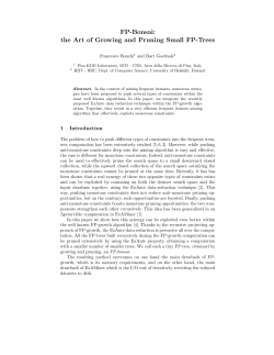
are right-angle triangles, with orthogonal sides parallel to the axes, and B is a box, as
in Figure 1. In a previous exercise it was shown that triangles are Jordan measurable.
A translation of T2 by the vector −(0, b) shows that T1 ] T2 has the Jordan measure of
the box Ii × Ii . Thus, P is Jordan measurable and has Jordan measure J(P ) = |Ii | · |Ij |,
which consequently is J(P ) = m(Ii × Ij ).
P
T2
B
T1
T1
T2 − (0, b)
Figure 1. Computation of the Jordan measure of the parallelepiped P .
24
Exercise 2.15. Let P := {(x, x + y) : x ∈ I, y ∈ J} where I, J are intervals. Show
that P is Jordan measurable and that J(P ) = |I| · |J|.
We conclude that Ri,j (B) is Jordan measurable, and that
J(Ri,j (B)) = J(S(P × B)) = J(P × B) = J2 (P ) · Jd−2 (B) = |Ii | · |Ij | ·
Y
k6=i,j
|Ik | = m(B),
where P = {(x, x + y) : x ∈ Ii , y ∈ Ij } and B = I3 × · · · Ii−1 × I1 × Ii+1 × · · · × Ij−1 ×
Ij × Ij+1 × · · · × Id ⊂ Rd−2 . Since | det Ri,j | = 1 we have just proved that for any box
B, the set Ri,j (B) is Jordan measurable and J(Ri,j (B)) = | det Ri,j | · m(B).
Just as for Mc,j and Si,j we now use the fact that Ri,j (A ] B) = Ri,j (A) ] Ri,j (B) to
prove the theorem for any L ∈ {Mc,j , Si,j , Ri,j }.
Finally, if L is a general invertible linear map, then L = L1 · · · Ln where Lk ∈
{Mc,j , Si,j , Ri,j } for all k. So for any A that is Jordan measurable, also Ln (A) is Jordan
measurable, and thus Ln−1 Ln (A) is as well, and so on to get that L(A) = L1 · · · Ln (A)
is Jordan measurable. We also compute the measure by
J(L(A)) = J(L1 (L2 · · · Ln (A))) = | det L1 | · J(L2 · · · Ln (A)) =
= · · · = | det L1 | · · · | det Ln | · J(A) = | det L| · J(A).
t
u
Number of exercises in lecture: 15
Total number of exercises until here: 21
25
Measure Theory
Ariel Yadin
Lecture 3: Lebesgue outer measure
3.1. From finite to countable
Recall that in order to measure sets from outside we used the outer measure by
approximating with finitely many elementary sets.
Exercise 3.1. Show that
J ∗ (A) =
inf
A⊂B1 ∪···∪Bn
m(B1 ) + · · · + m(Bn ),
where B1 , . . . , Bn are always boxes.
Lebesgue’s idea is that there is no reason to stop with finite, and not countable
collections. (Mathematicians are not afraid of infinity anymore...)
• Definition 3.1. Let A ⊂ Rd be a set. The Lebesgue outer measure of A is defined
to be
m∗ (A) := inf
X
n
|Bn | : (Bn )n is a sequence of boxes , A ⊂
[
Bn .
n
X Note that we may have m∗ (A) = ∞.
Exercise 3.2. Show that in general m∗ (A) ≤ J ∗ (A) for bounded sets A.
Show that for Q := Q ∩ [0, 1] we have that
J ∗ (Q) = 1
and
m∗ (Q) = 0.
26
♣ Solution to ex:3.2.
:(
If A is bounded then the infimum for Lebesgue outer measure is on a larger set than
the infimum for Jordan outer measure.
For Q, we have that Q = [0, 1], so J ∗ (Q) = J ∗ ([0, 1]) = m([0, 1]) = 1 and if Q =
P
{q1 , q2 , . . .} is an enumeration of Q then m∗ (Q) ≤ n | {qn } | = 0.
:) X
Exercise 3.3. Give an example of an unbounded set with Lebesgue outer measure
0.
• Proposition 3.2. Properties of Lebesgue outer measure:
• m∗ (∅) = 0.
• (Monotonicity) If A ⊂ C then m∗ (A) ≤ m∗ (C).
S
• (Countable subadditivity) If (An )n is a sequence of sets then m∗ ( n An ) ≤
P
∗
n m (An ).
Proof. First, ∅ is a box of volume 0; another proof is by noting that ∅ ⊂ [0, n1 ]d for all
n, so m∗ (∅) ≤ inf n m([0, n1 ]d ) = 0.
For A ⊂ C we have that the infimum used to obtain m∗ (A) is over a larger set that
the one used to obtain the infimum for m∗ (C).
Let (An )n be a sequence of sets. Fix ε > 0. For every n let (Bn,k )k be a sequence of
S
boxes such that An ⊂ k Bn,k and
X
k
|Bn,k | ≤ m∗ (An ) + ε · 2−n .
Consider the sequence of boxes (Bn,k )n,k . We have that
[
n
An ⊂
[
n,k
Bn,k ,
27
and so
m∗ (
[
n
An ) ≤
X
n,k
|Bn,k | ≤
X
m∗ (An ) +
n
X
n
ε · 2−n =
X
m∗ (An ) + 2ε.
n
Taking ε → 0 we have countable subadditivity.
t
u
It is now natural to ask for the additivity property: if A ∩ C = ∅ is it true that
m∗ (A ] C) = m∗ (A) + m∗ (C)? As it turns out, this is not always the case, a counter
example will be given in the future. However, in some cases, when the sets are separated
enough, we have additivity.
• Proposition 3.3. If A, C are such that dist(A, C) > 0 then m∗ (A ] C) = m∗ (A) +
m∗ (C).
Specifically, if A, C are closed disjoint sets and A is compact then dist(A, C) > 0.
Proof. By sub-additivity it suffices to prove m∗ (A) + m∗ (C) ≤ m∗ (A ] C). We may also
assume w.l.o.g. that m∗ (A]C) < ∞ and by monotonicity that m∗ (A) < ∞, m∗ (C) < ∞.
S
P
Fix ε > 0. Let (Bn )n be a sequence of boxes such that A ] C ⊂ n Bn and n |Bn | ≤
m∗ (A ] C) + ε.
Let r = dist(A, C) > 0. Note that for any n, we may replace the box Bn by a finite
number of disjoint boxes Bn,1 , . . . , Bn,k such that the diameter of any Bn,j is less than r.
P
S
So we obtain a sequence (Bn0 )n such that A ] C ⊂ n Bn0 and n |Bn0 | ≤ m∗ (A ] C) + ε,
and such that any box Bn0 cannot intersect both A and C.
Thus, we have that N = NA ] NC where NA = {n : Bn0 ∩ A 6= ∅} and NC =
{n : Bn0 ∩ C 6= ∅}.
We now have that
A⊂
[
Bn0
and
n∈NA
C⊂
[
Bn0 ,
n∈NC
and so
m∗ (A) + m∗ (C) ≤
X
n∈NA
|Bn0 | +
Taking ε → 0 completes the proof.
X
n∈NC
|Bn0 | ≤
X
n
|Bn0 | ≤ m∗ (A ] C) + ε.
28
As for the case where A, C are closed and A is compact, note that dist(x, C) is a
continuous function of x (because C is closed) and so achieves a minimum on A when
t
u
A is compact.
Exercise 3.4. Give an example of two closed sets A, C such that A ∩ C = ∅ but
dist(A, C) = 0.
The next proposition shows that the notation “m” is an appropriate one, as an extension of elementary measure.
• Proposition 3.4. For any elementary set E we have that m∗ (E) = m(E).
Proof. If suffices to prove that J ∗ (E) ≤ m∗ (E).
Case I. E is closed. Since E is bounded, it is compact, and the Heine-Borel Theorem
tells us that every open cover of E has a finite sub-cover.
Fix any ε > 0. Let (Bn )n be a sequence of boxes such that E ⊂
S
n Bn
and
m∗ (E) + ε.
P
n |Bn |
≤
X The boxes (Bn )n do not form an open cover – they need not be open.
For every n let Bn0 be an open box containing Bn ⊂ Bn0 such that |Bn0 | ≤ |Bn | + ε2−n .
P
(Exercise: show this is possible.) Then, n |Bn0 | ≤ m∗ (E) + 2ε and (Bn0 )n are an open
cover of E. Thus, there is a finite sub-cover
E⊂
N
[
Bn0 ,
n=1
for some large enough N . Thus,
∗
J (E) ≤
N
X
n=1
|Bn0 | ≤
X
n
|Bn0 | ≤ m∗ (E) + 2ε.
Taking ε → 0 completes the proof for closed E.
Case II. E is a general elementary set. Write E = B1 ] · · · ] Bn where (Bj )nj=1 are
disjoint boxes. These need not be closed boxes.
29
Fix ε > 0. For every 1 ≤ j ≤ n let Bj0 ⊂ Bj be a closed box such that |Bj0 | ≥ |Bj | − nε .
(Exercise: Show this is always possible.) Then, E 0 = B10 ] · · · ] Bn0 is a finite union of
disjoint closed boxes, and thus a closed elementary set. Also,
0
m(E ) =
n
X
j=1
|Bj0 |
≥
n
X
j=1
|Bj | − ε = m(E) − ε.
So by Case I,
m(E) ≤ m(E 0 ) + ε = m∗ (E 0 ) + ε ≤ m∗ (E) + ε.
Taking ε → 0 completes the proof.
t
u
Exercise 3.5. Show that for any bounded set A we have
J∗ (A) ≤ m∗ (A) ≤ J ∗ (A).
Show that if A is Jordan measurable then m(A) = m∗ (A).
♣ Solution to ex:3.5.
:(
We have already seen m∗ (A) ≤ J ∗ (A). If E is an elementary set such that E ⊂ A, then
m(E) = m∗ (E) ≤ m∗ (A) by monotonicity. Taking supremum over all such elementary
sets contained in A, we get that J∗ (A) ≤ m∗ (A). This proves the first assertion.
If A is Jordan measurable, then m(A) = J∗ (A) ≤ m∗ (A) ≤ J ∗ (A) = m(A).
Number of exercises in lecture: 5
Total number of exercises until here: 26
:) X
30
Measure Theory
Ariel Yadin
Lecture 4: Lebesgue measure
4.1. Definition of Lebesgue measure
Recall that A is Jordan measurable if and only if for every ε > 0 there exists an
elementary set E such that A ⊂ E and J ∗ (E \ A) < ε. This motivates the following.
Later we will see that there is another way to approach the issue of Lebesgue measure,
and outer measures in general.
• Definition 4.1 (Lebesgue measure). A set A ⊂ Rd is said to be Lebesgue measur-
able if for every ε > 0 there exists an open set U such that A ⊂ U and m∗ (U \ A) < ε.
for Lebesgue measurable A we denote m(A) := m∗ (A) and refer to this as the
Lebesgue measure of A.
X Lebesgue measurable sets are sets that are “almost open”.
?
Why do open sets enter the picture?
• Definition 4.2. We say that boxes (Bn )n are almost disjoint if any two boxes can
◦ = ∅.
only intersect at their boundary; that is, for every n 6= m, Bn◦ ∩ Bm
• Lemma 4.3. Any open set U ⊂ Rd can be written as a countable union of almost
disjoint closed boxes.
Proof. For any z ∈ Zd define the dyadic cube at scale n ≥ 0:
Dn (z) =
z
1
2n
, z12+1
× · · · × 2znd , zd2+1
.
n
n
This is the d-dimensional cube of side-lengths 2−n and corner z.
The following is the crucial property to verify: If Dn (z)◦ ∩ Dm (z 0 )◦ 6= ∅ then one is
contained in the other.
31
Specifically, if Dn (z) ( Dm (z 0 ) then n > m.
Now, set
n
o
Γ = (z, n) : z ∈ Zd , n ≥ 0, Dn (z) ⊂ U .
These are all dyadic cubes whose closure is contained in U . Also, set
Λ = (z, n) ∈ Γ : 6 ∃ (z 0 , n0 ) ∈ Γ , Dn (z) ⊂ Dn0 (z 0 ) .
These are all dyadic cubes contained in U that are maximal with respect to inclusion.
We claim that
[
U=
Dn (z).
(z,n)∈Λ
One inclusion is obvious, since all closures of dyadic cubes indexed by Λ are contained
in U . For the other inclusion, let x ∈ U . Then, since U is open (this is the only place
we use that U is an open set!), there is a small ball B(x, ε) ⊂ U . However, for large
√
enough n (so that d2−n < ε), if x ∈ Dn (z) then Dn (z) ⊂ B(x, ε) ⊂ U (because Dn (z)
√
has diameter d2−n ). Since for every n there exists some dyadic cube of scale n that
S
contains x (because Rd = z∈Zd Dn (z) for every fixed n), we get that for some large
enough n there exists z ∈ Zd with (z, n) ∈ Γ and x ∈ Dn (z). Thus, there must be
(z, n) ∈ Λ such that x ∈ Dn (z) (by just taking the cube of minimal scale containing x).
Since this holds for all x ∈ U we get that
U⊂
[
Dn (z).
(z,n)∈Λ
This is of course a countable union. Also, since Λ is the indices of maximal dyadic
cubes, any two cannot intersect except for the boundary; that is, they are almost disjoint.
t
u
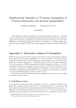
This construction has a remarkable consequence.
Exercise 4.1. Show that if U =
P
then m∗ (U ) = n |Bn | = J∗ (U ).
S
n Bn
where (Bn )n are almost disjoint boxes
32
Figure 2. Part of the dyadic decomposition of a set. If the set is open,
one can continue to capture all points in the set by taking smaller and
smaller squares.
♣ Solution to ex:4.1. :(
P
P
P
m∗ (U ) ≤ n |Bn | so it suffices to show that n |Bn | ≤ J∗ (U ). Note that m
n=1 |Bn | ≤
P
J∗ (U ) for all m because B1 ∪ · · · ∪ Bm ⊂ U . Taking m → ∞ we have n |Bn | ≤ J∗ (U ).
:) X
Exercise 4.2. Show that if (Bn )n are almost disjoint and (Bn0 )n are almost disjoint,
S
S
and if n Bn = n Bn0 then
X
X
|Bn | =
|Bn0 |.
n
n
• Proposition 4.4 (Outer regularity, Lebesgue measure). For any set A we have
m∗ (A) =
inf
A⊂U open
m∗ (U ).
Proof. One direction m∗ (A) ≤ m∗ (U ) for any open U ⊃ A, is just monotonicity.
33
For the other direction, if m∗ (A) = ∞ there is nothing to prove. Assume m∗ (A) < ∞.
S
P
Fix ε > 0. Let (Bn )n be boxes such that A ⊂ n Bn and n |Bn | ≤ m∗ (A) + ε. For
every n let Bn0 be an open box such that Bn ⊂ Bn0 and |Bn0 | ≤ |Bn | + ε2−n . Thus, the
S
set U = n Bn0 is an open set containing A and
m∗ (U ) ≤
X
n
|Bn0 | ≤ m∗ (A) + 2ε.
Taking infimum over the left hand side and ε → 0 completes the proof.
t
u
Exercise 4.3. Show that it is false that
m∗ (A) =
sup
m∗ (U ).
A⊃U open
• Proposition 4.5 (Lebesgue measurable sets). Examples of Lebesgue measurable sets:
• If U is open it is Lebesgue measurable.
• If m∗ (A) = 0 then A is Lebesgue measurable.
• ∅ is Lebesgue measurable.
• If (An )n is a sequence of Lebesgue measurable sets, then
S
n An
is Lebesgue
T
n An
is Lebesgue
measurable.
• Any closed set F is Lebesgue measurable.
• If A is Lebesgue measurable then so is Ac = Rd \ A.
• If (An )n is a sequence of Lebesgue measurable sets, then
measurable.
Proof. For open sets this is obvious by definition.
If m∗ (A) = 0 then by outer regularity for any ε > 0 there exists an open set U ⊃ A
such that m∗ (U \ A) ≤ m∗ (U ) < m∗ (A) + ε = ε. So A is Lebesgue measurable.
∅ has m∗ (∅) ≤ J ∗ (∅) = 0.
34
Countable unions. Now, if (An )n are all Lebesgue measurable, then: Fix ε > 0.
For every n there exists an open set Un ⊃ An such that m∗ (Un \ An ) < ε2−n . Thus,
S
S
U := n Un is an open set containing n An such that by subadditivity,
m∗ (U \
[
n
An ) ≤
Since this holds for all ε > 0 we get that
X
S
n
µ∗ (Un \ An ) ≤ ε.
n An
is Lebesgue measurable.
S
Closed sets. Let F be a closed set. Note that F = n (F ∩ B[0, n]) where B[0, n]
is the closed ball of radius n. So it suffices to prove that F is Lebesgue measurable
for closed and bounded F (because then F ∩ B[0, n] is Lebesgue measurable for all n).
Heine-Borel guaranties then that F is compact.
Fix ε > 0. Let U be an open set such that F ⊂ U and m∗ (U ) ≤ m∗ (F ) + ε. The
S
set U \ F is open, so we can write U \ F = n Bn where (Bn )n are almost disjoint and
closed boxes. For any m > 0, the set Cm := B1 ∪ · · · ∪ Bm is closed and disjoint from
F . Also, F is compact, so we have additivity:
m∗ (F ) + m∗ (Cm ) = m∗ (F ∪ Cm ) ≤ m∗ (F ∪ (U \ F )) = m∗ (U ) ≤ m∗ (F ) + ε.
Since F is bounded, we have that m∗ (F ) < ∞, so we conclude that for all m > 0,
m
X
n=1
|Bn | = m∗ (B1 ∪ · · · ∪ Bm ) ≤ ε,
where the equality is because (Bn )n are almost disjoint. Thus, taking m → ∞,
m∗ (U \ F ) =
X
n
|Bn | ≤ ε.
This holds for all ε > 0, so F is Lebesgue measurable.
Complements. Now, if A is Lebesgue measurable: For every n let Un ⊃ A be an
S
open set such that m∗ (Un \ A) < 2−n . Let Fn = Unc and let F = n Fn . Since Fn are
closed they are Lebesgue measurable, and thus F is Lebesgue measurable as a countable
union. Note that m∗ (Ac \ Fn ) = m∗ (Un \ A) < 2−n for all n. Since Ac \ F ⊂ Ac \ Fn ,
m∗ (Ac \ F ) ≤ inf m∗ (Ac \ Fn ) = 0.
n
Thus, Ac = F ∪ (Ac \ F ) which is the union of two Lebesgue measurable sets, and thus
Lebesgue measurable itself.
35
Countable intersections. If (An )n are all Lebesgue measurable, then so are (Acn )n
and thus also
!c
\
n
An =
[
Acn
.
n
t
u
Exercise 4.4. Show that the following are equivalent.
(1) A is Lebesgue measurable.
(2) For every ε > 0 there exists an open set U ⊃ A such that m∗ (U \ A) < ε.
(3) For every ε > 0 there exists an open set U such that m∗ (U 4A) < ε.
(4) For every ε > 0 there exists a closed set F such that m∗ (A4F ) < ε.
(5) For every ε > 0 there exists a closed set F ⊂ A such that m∗ (A \ F ) < ε.
(6) For every ε > 0 there exists a Lebesgue measurable set C such that m∗ (A4C) <
ε.
♣ Solution to ex:4.4.
:(
(1) ⇐⇒ (2) is the definition.
(2) ⇒ (3) follows by taking the same open set U ⊃ A.
(3) ⇒ (2): Fix ε > 0 and let U be such that m∗ (U 4A) < ε. Let V ⊃ U 4A be an
open set such that m∗ (V ) < 2ε, by outer regularity. Note that A ⊂ U ∪ (A \ U ) ⊂ U ∪ V ,
which is an open set, and
m∗ ((U ∪ V ) \ A) ≤ m∗ (U \ A) + m∗ (V \ A) ≤ m∗ (U 4A) + m∗ (V ) < 3ε.
So (1) ⇐⇒ (2) ⇐⇒ (3).
(1) ⇒ (4): A is Lebesgue measurable, so also Ac is. Fix ε > 0 and let U be an open
set such that m∗ (U 4Ac ) < ε. Let F = U c . So m∗ (F 4A) = m∗ (U 4Ac ) < ε, and F is
closed.
(4) ⇒ (5): Fix ε > 0 and let F be a closed set such that m∗ (A4F ) < ε. By outer
regularity let U ⊃ A4F be an open set such that m∗ (U ) < 2ε. Then F ∩ U c is a closed
36
set and F ∩ U c ⊂ F ∩ A ⊂ A, and
m∗ (A \ F ∩ U c ) ≤ m∗ (A \ F ) + m∗ (A \ U c ) ≤ m∗ (A4F ) + m∗ (U ) < 3ε.
(5) ⇒ (6): Fix ε > 0 and let F ⊂ A be a closed set such that m∗ (A \ F ) < ε. The
C = F is Lebesgue measurable, and m∗ (A4C) = m∗ (A \ F ) < ε.
(6) ⇒ (3): Fix ε > 0 and let C be Lebesgue measurable such that m∗ (A4C) < ε.
Let U ⊃ C be an open set such that m∗ (U 4C) = m∗ (U \ C) < ε. Note that A4U ⊂
S
A4C C4U , so
m∗ (A4U ) ≤ m∗ (A4C) + m∗ (C4U ) < 2ε.
:) X
Exercise 4.5. Show that if A is Jordan measurable then it is also Lebesgue mea-
surable.
• Definition 4.6. A family of subsets F is a σ-algebra if
• ∅ ∈ F;
• F is closed under complements, i.e. A ∈ F implies Ac ∈ F;
• F is closed under countable unions, i.e. (An )n ⊂ F implies
S
n An
∈ F.
Exercise 4.6. Show that if F is a σ-algebra it is closed under countable intersec-
tions, set difference and symmetric difference.
Exercise 4.7. Show that the family of Lebesgue measurable sets form a σ-algebra.
37
4.2. Lebesgue measure as a measure
• Proposition 4.7 (Measure axioms). Let L be the family of all Lebesgue measurable
sets. Recall that for A ∈ L we define m(A) = m∗ (A). We the have that m : F → [0, ∞]
with the following properties:
• m(∅) = 0;
• (Countable additivity) If (An )n ⊂ L are pairwise disjoint Lebesgue measurable
sets then
m(
]
An ) =
n
X
m(An ).
n
Proof. We only need to prove the assertion regarding additivity.
Case I. (An )n are all compact. Since m∗ is additive on disjoint compact sets, for any
N,
N
X
m(An ) = m(
n=1
N
]
n=1
An ) ≤ m(
]
n
An ) ≤
X
m(An ),
n
where the last two inequalities are monotonicity and countable subadditivity. Taking
N → ∞ we get the compact case.
Case II. (An )n are all bounded. Fix ε > 0. For every n let Fn be a closed set with
Fn ⊂ An and m∗ (An \ Fn ) < ε2−n . Since Fn ⊂ An is bounded, Fn is compact. By
subadditivity, m(An ) ≤ m(Fn ) + ε2−n , so
X
n
m(An ) ≤
X
n
]
]
m(Fn ) + ε = m( Fn ) + ε ≤ m( An ) + ε.
n
n
Taking ε → 0 completes the bounded case.
Case III. Now for the general case. Let Ck = B(0, k) \ B(0, k − 1) for all n, and
set Dn,k = An ∩ Ck . So (Dn,k )n,k is a sequence of pairwise disjoint bounded Lebesgue
measurable sets. Thus, for every n,
]
X
m(An ) = m( Dn,k ) =
m(Dn,k ),
k
k
and
m(
]
n
An ) = m(
]
n,k
Dn,k ) =
X
n,k
m(Dn,k ) =
X
m(An ).
n
t
u
38
Exercise 4.8. Show that if A is Lebesgue measurable then
m(A) =
sup
m(K).
A⊃K compact
♣ Solution to ex:4.8.
:(
Monotonicity implies that it suffices to prove that m(A) ≤ supA⊃K
compact
m(K).
First suppose that A is bounded, so m(A) < ∞.
Fix ε > 0. Since A is Lebesgue measurable there exists a closed set K ⊂ A such that
µ∗ (A \ K) < ε. Since K ⊂ A and A is bounded, we have that K is bounded as well, so
K is compact because it is bounded and closed. So K is a compact set such that K ⊂ A
and µ(K) = µ(A) − µ(A \ K) ≥ µ(A) − ε. This holds for all ε > 0 establishing the claim
in the case that A is bounded.
For the case where A is unbounded, consider An = A ∩ (B(0, n) \ B(0, n − 1)) for all n.
These are all bounded, so for every ε > 0 and every n there exists a compact set Kn ⊂ An
P
such that m(Kn ) ≥ m(An )−ε2−n . Also, (An )n are disjoint so m(A) = n m(An ). Thus,
U
if Kn0 = nj=1 Kj , then Kn0 is compact, Kn0 ⊂ A and
m(Kn0 )
=
n
X
j=1
m(Kj ) ≥
n
X
j=1
m(Aj ) − ε → m(A) − ε.
This implies that there exists n large enough so that m(Kn0 ) ≥ m(A) − 2ε.
Conclusion, for any ε > 0 there exists a compact K ⊂ A such that m(K) ≥ m(A) − ε.
This proves the unbounded case.
Finally, let us end with the following criterion for Lebesgue measurability.
• Proposition 4.8 (Charathéodory criterion). The following are equivalent.
• A is Lebesgue measurable.
• For every box B we have |B| = m∗ (B ∩ A) + m∗ (B \ A).
• For every elementary set E we have m(E) = m∗ (E ∩ A) + m∗ (E \ A).
:) X
39
Proof. If A is Lebesgue measurable and E is elementary, then E = (E∩A)](E\A) which
are both Lebesgue measurable sets, so by additivity, m(E) = m∗ (E ∩ A) + m∗ (E \ A).
U
Suppose the second bullet holds. Let E be any elementary set, and write E = nj=1 Bj
for disjoint boxes (Bj )nj=1 . Then by subadditivity,
∗
∗
m (E ∩ A) + m (E \ A) ≤
n
X
j=1
∗
∗
m (Bj ∩ A) + m (Bj \ A) =
n
X
j=1
|Bj | = m(E).
Since m(E) ≤ m∗ (E ∩ A) + m∗ (E \ A) for any set E just by subadditivity, we conclude
that equality holds for all elementary sets, proving the third bullet.
Now assume the third bullet. We want to show that A is Lebesgue measurable.
Assume first that m∗ (A) < ∞. Fix ε > 0. Let (Bn )n be disjoint boxes such that
S
∗
∗
n |Bn | ≤ m (A) + ε and A ⊂
n Bn (this exists by the definition of m ). For every n
S
let Bn0 ⊃ Bn be an open box such that |Bn0 | ≤ |Bn | + ε2−n . Note that U = n Bn0 is an
P
open set and U ⊃ A. For every n we have that
m∗ (Bn0 ∩ A) + m∗ (Bn0 \ A) = |Bn0 | ≤ |Bn | + ε2−n .
By subadditivity,
m∗ (A) + m∗ (U \ A) ≤
Thus,
m∗ (U
X
n
m∗ (Bn0 ∩ A) + m∗ (Bn0 \ A) ≤
X
n
|Bn | + ε ≤ m∗ (A) + 2ε.
\ A) ≤ 2ε. Since this holds for all ε > 0 this completes the proof for A with
m∗ (A) < ∞.
Now assume that m∗ (A) = ∞. Let E be any elementary set, and let B be a box.
Since E ∩ B is elementary, and since E \ (A ∩ B) ⊆ (E \ B) ∪ ((E ∩ B) \ A), we have that
m∗ (E ∩ A ∩ B) + m∗ (E \ (A ∩ B)) ≤ m∗ (E ∩ B ∩ A) + m∗ ((E ∩ B) \ A) + m(E \ B)
= m(E ∩ B) + m(E \ B) = m(E).
Thus, for any elementary E we have the Carathéodory criterion for A ∩ B,
m(E) = m∗ (E ∩ (A ∩ B)) + m∗ (E \ (A ∩ B)).
Since B is bounded, we have m∗ (A∩B) < ∞ and by the previous part A∩B is Lebesgue
S
measurable. Since A = n (A ∩ Bn ) where Bn are boxes of side length n around 0, we
40
have that A is Lebesgue measurable as a countable union of Lebesgue measurable sets.
t
u
Exercise 4.9. For a bounded set A define the Lebesgue inner measure by
m∗ (A) = m(E) − m∗ (E \ A),
for a Lebesgue mesurable set E such that A ⊂ E and m(E) < ∞.
Show that this definition does not depend on the choice of the set E.
Show that m∗ (A) ≤ m∗ (A) and equality holds if and only if A is Lebesgue measurable.
♣ Solution to ex:4.9.
:(
Let E, F be Lebesgue measurable sets such that A ⊂ F ⊂ E and m(E) < ∞.
P
S
Fix ε > 0. Let (Bn )n be a sequence of boxes such that E \ A ⊂ n An and n |Bn | ≤
m∗ (E \ A) + ε. Note that
F \ A ⊂ (E \ A) \ (E \ F ) ⊂
[
n
(Bn \ (E \ F ))
and
E\F ⊂
[
(Bn ∩ (E \ F )).
n
So,
m(E \ F ) + m∗ (F \ A) ≤
=
X
n
X
n
m∗ (Bn ∩ (E \ F )c ) + m∗ (Bn ∩ (E \ F ))
|Bn | ≤ m∗ (E \ A) + ε.
Taking ε → 0 and rearranging we have that
m(E) − m∗ (E \ A) ≤ m(F ) − m∗ (F \ A).
Since E \ A ⊂ (E \ F ) ∪ (F \ A) we have
m(E) − m∗ (E \ A) ≥ m(E) − m(E) + m(F ) − m∗ (F \ A).
So we have show that
m(E) − m∗ (E \ A) = m(F ) − m(F \ A)
41
whenever A ⊂ F ⊂ E.
For general Lebesgue measurable sets E, F such that A ⊂ F and A ⊂ E and m(E) <
∞, m(F ) < ∞, we have that A ⊂ E ∩ F , so
m(E) − m∗ (E \ A) = m(E ∩ F ) − m∗ ((E ∩ F ) \ A) = m(F ) − m∗ (F \ A).
This shows that m∗ is well defined.
Now, if A is Lebesgue measurable then for any Lebesgue measurable set E ⊃ A with
m(E) < ∞ we have that m(E \ A) = m(E) − m(A). So m∗ (A) = m(E) − m(E \ A) =
m(A) = m∗ (A).
On the other hand, assume that m∗ (A) = m∗ (A). Fix ε > 0 and let U ⊃ A be an
open set such that A ⊂ U and m(U ) ≤ m∗ (A) + ε. Note that
m(U ) − ε ≤ m∗ (A) = m∗ (A) = m(U ) − m∗ (U \ A),
so m∗ (U \ A) ≤ ε.
:) X
T
where (Un )n are all open
S
(i.e. a countable intersection of open sets). A Fσ set is a set A = n Fn where (Fn )n
Exercise 4.10. Reminder: A Gδ set is a set A =
n Un
are all closed (i.e. a countable union of closed sets).
A null set is a set with Lebesgue (outer) measure 0.
Show that the following are equivalent.
• A is Lebesgue measurable.
• A = G \ N is where G is Gδ and N is null.
• A = F ∪ N where F is Fσ and N is null.
Exercise 4.11. Show that if A is Lebesgue measurable then A + x is also Lebesgue
measurable and m(A + x) = m(A).
42
Exercise 4.12.
m0
Let L be the family of Lebesgue measurable sets. Suppose that
: L → [0, ∞] admits the following properties:
• m0 (∅) = 0;
U
• If (An )n ⊂ L are pairwise disjoint Lebesgue measurable sets then m0 ( n An ) =
P
0
n m (An );
• m0 (A + x) = m0 (A) for all A ∈ L, x ∈ Rd ;
• m0 ([0, 1]d ) = 1.
Show that m0 is Lebesgue measure.
♣ Solution to ex:4.12.
:(
We already know that m0 (E) = m(E) for any Jordan measurable set E, and specifically
for boxes.
It is simple to prove that m0 is sub-additive and monotone.
Step I. We show that for A ∈ L, if m(A) = 0 then m0 (A) = 0: Let A be a Lebesgue
measurable set of 0 measure, m(A) = 0. For any ε > 0, let (Bn )n be a sequence of
S
P
P
boxes such that A ⊂ n Bn and such that n |Bn | ≤ ε. Then, m0 (A) ≤ n m0 (Bn ) =
P
0
n |Bn | ≤ ε, and taking ε → 0, we have that m (A) = 0.
Step II. We show that if U is open of finite Lebesgue measure, then m0 (U ) = m(U ):
S
Let U be an open set such that m(U ) < ∞. Write U = n Bn where (Bn )n are
almost disjoint closed boxes. Let Bn0 = (Bn )◦ , so (Bn0 )n are pairwise disjoint. Let
S
U
F = n Bn \ n Bn0 . Since
m(F ) = m(U ) − m(
]
Bn0 ) =
n
n
we have that m0 (F ) = 0. Note that U = F ]
m0 (U ) = m0 (F ) +
X
X
n
U
|Bn | −
0
n Bn ,
m0 (Bn0 ) =
X
n
|Bn0 | = 0,
so
X
n
|Bn0 | = m(U ).
43
Step III. We show that for any A ∈ L, the inequality m0 (A) ≤ m(A) holds: Let A
be a Lebesgue measurable set with m(A) < ∞. Fix ε > 0 and let U be an open set such
that A ⊂ U and m(U ) − m(A) = m(U \ A) < ε. Then, m0 (A) ≤ m0 (U ) ≤ m(A) + ε.
Taking ε → 0 we have that for any A ∈ L, the inequality m0 (A) ≤ m(A) holds. (The
case where m(A) = ∞ is immediate.)
Step IV. We show that for any bounded set A ∈ L we have m0 (A) = m(A): Let A ∈ L
be a bounded set. Let B be a box bounding A ⊂ B. We have m0 (B \A) = m0 (B)−m0 (A)
by additivity of m0 . Also,
m0 (A) ≤ m(A) = m(B) − m(B \ A) ≤ m0 (B) − m0 (B \ A) = m0 (A).
Step V. We show that for any A ∈ L we have m0 (A) = m(A): Let A ∈ L. Write
U
A = An where An = Bn \ Bn−1 , and Bn = [−n, n]d . Then by additivity of both m, m0
and since An are all bounded,
m0 (A) =
X
m0 (An ) =
n
X
m(An ) = m(A).
n
:) X
Number of exercises in lecture: 12
Total number of exercises until here: 38
44
Measure Theory
Ariel Yadin
Lecture 5: Abstract measures
We now review the construction of Lebesgue measure, isolating the main abstract
properties, in order to generalize it to other settings.
5.1. σ-algebras
We saw in the discussion of Lebesgue measure that the family of Lebesgue measurable
sets form a special structure called a σ-algebra.
• Definition 5.1 (σ-algebra). Let X be any set.
We denote by 2X = P(X) =
{A : A ⊂ X} the set of all subsets of X.
A family F ⊂ 2X is called a σ-algebra (on X) if:
• ∅ ∈ F;
• F is closed under complements, i.e. A ∈ F implies X \ A ∈ F;
• F is closed under countable unions, i.e. if (An )n is a sequence in F then
S
n An
∈
F.
Exercise 5.1. Show that if F is a σ-algebra on X then:
• F is closed under countable intersections, i.e. if (An )n is a sequence in F then
T
n An ∈ F.
• X ∈ F.
• F is closed under finite unions and finite intersections.
• F is closed under set differences.
• F is closed under symmetric differences.
45
Exercise 5.2. Suppose F ⊂ 2X is a family of subsets satisfying the following:
• ∅ ∈ F;
• F is closed under complements;
• F is closed under countable intersections.
Show that F is a σ-algebra.
Exercise 5.3. Show that if (Fα )α∈I is a collection of σ-algebras on X, then
T
α Fα
is also a σ-algebra on X.
• Proposition 5.2 (σ-algebra generated by subsets). Let K be a collection of subsets
of X.
There exists a σ-algebra, denoted σ(K) such that K ⊂ σ(K) and for every other σalgebra F such that K ⊂ F we have that σ(K) ⊂ F.
That is, σ(K) is the smallest σ-algebra containing K.
We call σ(K) the σ-algebra generated by K.
Proof. Define
σ(K) :=
\
{F : F is a σ-algebra on X , K ⊂ F} .
This is a σ-algebra with the required properties.
t
u
Exercise 5.4. Show that if K ⊂ L then σ(K) ⊂ σ(L). Also, if K ⊂ F and F is a
σ-algebra, then σ(K) ⊂ F.
46
• Definition 5.3 (Borel σ-algebra). Given a topological space X, the Borel σ-algebra
is the σ-algebra generated by the open sets. It is denoted B(X).
Specifically in the case X = Rd we have that
B = Bd = B(Rd ) = σ(U : U is an open set ).
X A Borel-measurable set, i.e. a set in B(X), is called a Borel set.
Exercise 5.5. Prove that
B = Bd = B(Rd ) = σ(B : B is an open box ) = σ(B 0 : B 0 is a closed box ).
♣ Solution to ex:5.5.
:(
If B is an open box then B ∈ B so σ(B : B is an opend box ) ⊂ B.
If U is an open set then it is a countable union of closed boxes, so U ∈ σ(B
:
B is a closed box ), which shows that B ⊂ σ(B 0 : B 0 is a closed box ).
If B 0 = [a1 , b1 ] × · · · × [ad , bd ] is a closed box, then for
Bn = (a1 − n1 , b1 + n1 ) × · · · × (ad − n1 , bd + n1 ),
we have that B 0 =
T
n Bn
and Bn are all open boxes. Thus, B 0 ∈ σ(B : B is an open box ),
which implies that σ(B 0 : B 0 is a closed box ) ⊂ σ(B : B is an open box ).
:) X
47
Exercise 5.6. Show that
B(R) = σ((a, b) : −∞ < a < b < ∞) = σ([a, b] : −∞ < a < b < ∞)
= σ((a, b] : −∞ < a < b < ∞) = σ([a, b) : −∞ < a < b < ∞)
= σ((a, ∞) : −∞ < a < ∞) = σ([a, ∞) : −∞ < a < ∞)
= σ((−∞, a) : −∞ < a < ∞) = σ((−∞, a] : −∞ < a < ∞).
5.2. Measures
• Definition 5.4. A pair (X, F) where F is a σ-algebra on X is call a measurable
space. Elements of F are called measurable sets.
Given a measurable space (X, F), a function µ : F → [0, ∞] is called a measure (on
(X, F)) if
• µ(∅) = 0;
• (Additivity) For all sequences (An )n ⊂ F of pairwise disjoint sets in F, we have
that
]
X
µ( An ) =
µ(An ).
n
n
(X, F, µ) is called a measure space.
X A measure space (X, F, µ) is called finite if µ(X) < ∞. It is called σ-finite if
S
X = n An where An ∈ F and µ(An ) < ∞ for all n.
Exercise 5.7. Show that any measure is finitely additive; that is, if (X, F, µ) is a
measure space then for any disjoint sets A, B ∈ F we have µ(A ] B) = µ(A) + µ(B).
48
Example 5.5. The counting measure: Take F = 2X and µ(A) = |A|.
If f : X → [0, ∞) is a function then
µ(A) :=
sup
X
f (an )
(an )n ⊂A n
is a measure on (X, 2X ).
If X is uncountable and
F = {A ⊂ X : A is countable, or Ac is countable } ,
then (X, F) is a measurable space and


1 Ac is countable
µ(A) =

0 A is countable
is a measure on (X, F).
454
Exercise 5.8. Give an example of a set X such that


∞ |A| = ∞,
µ(A) :=

0 |A| < ∞,
is not a measure on (X, 2X ).
• Proposition 5.6 (Basic properties of measures). Let (X, F, µ) be a measure space.
Then:
• (Monotonicity) For A ⊂ B ∈ F we have µ(A) ≤ µ(B).
S
P
• (Subadditivity) If (An )n ⊂ F then µ( n An ) ≤ n µ(An ).
Proof. Monotonicity follows from B = A ] (B \ A) and finite additivity, so µ(B) =
µ(A) + µ(B \ A) ≥ µ(A).
49
For subadditivity, let (An )n ⊂ F and set
n−1
[
Bn = An \ (
Aj ).
j=1
So
]
Bn =
n
[
An
and
n
B n ⊂ An .
Thus,
X
X
]
[
µ(An ).
µ(Bn ) ≤
µ( An ) = µ( Bn ) =
n
n
n
n
t
u
• Definition 5.7. For a measure space (X, F, µ) a set N ∈ F is called a null set (or
µ-null set) if µ(N ) = 0.
A measure space (X, F, µ) such that for all null sets N ∈ F we have that any A ⊂ N
is also measurable (i.e. in F) is called complete.
Exercise 5.9.
Let (X, F, µ) be a measure space. Let N be the set of all µ-null
sets. Define
F̄ := {A ∪ F : A ∈ F , F ⊂ N ∈ N } .
Show that F̄ is a σ-algebra.
Show that if we define µ̄ : F̄ → [0, ∞] by
µ̄(A ∪ F ) = µ(A)
∀ A ∈ F, F ⊂ N ∈ N ,
then µ̄ is a well defined complete measure on F̄; moreover, µ̄F = µ and if ν is a complete
measure on F̄ such that ν F = µ then ν = µ̄.
Exercise 5.10. Show that if µ1 , . . . , µn are measures on (X, F) the for any nonP
negative numbers a1 , . . . , an the function µ := j aj µj is also a measure on (X, F).
50
5.3. Fatou’s Lemma and continuity
• Proposition 5.8 (Monotone convergence). Let (X, F, µ) be a measure space.
If A1 ⊂ A2 ⊂ · · · is an increasing sequence in F then
[
lim µ(An ) = µ( An ).
n→∞
n
If A1 ⊃ A2 ⊃ · · · is an decreasing sequence in F then under the condition that there
exists n such that µ(An ) < ∞ we have that
\
lim µ(An ) = µ( An ).
n→∞
n
Proof. For the increasing sequence case define Bn = An \An−1 . Then, (Bn )n are pairwise
disjoint, so
lim µ(An ) = lim µ(
n→∞
n→∞
=
X
n
]
Bj ) = lim
n→∞
j=1
n
X
µ(Bj )
j=1
]
[
µ(Bn ) = µ( Bn ) = µ( An ).
n
n
n
For the decreasing sequence case, since µ(Ak ) < ∞ we define Bn = Ak \An (so Bn = ∅
if n ≤ k). Note that µ(Bn ) + µ(An ) = µ(Ak ) for n ≥ k and since µ(An ) ≤ µ(Ak ) < ∞
we have that µ(Bn ) = µ(Ak ) − µ(An ). Note that (Bn )n≥k is an increasing sequence such
S
T
T
that n≥k Bn = Ak \ n≥k An . Since n≥k An ⊂ Ak we have
µ(Ak ) = µ(
\
An ) + µ(
n≥k
[
\
Bn ) = µ( An ) + lim µ(Bn )
n
n≥k
n→∞
\
= µ( An ) + lim (µ(Ak ) − µ(An )).
n→∞
n
Since µ(Ak ) < ∞ we may subtract it from both sides to get the proposition.
Let (An )n be a sequence of subsets of X. Define
lim sup An =
\[
n k≥n
Ak
and
lim inf An =
[\
n k≥n
Ak .
t
u
51
lim sup An is the set of all x ∈ X that appear in infinitely many of the subsets An .
Similarly, lim inf An is the set of all x ∈ X that appear in all but finitely many of the
subsets An .
We say that the sequence (An )n converges if lim inf An = lim sup An , and denote this
common set by lim An = lim sup An = lim inf An in this case.
Exercise 5.11. Show that lim inf An ⊆ lim sup An .
Exercise 5.12. Show that if (An )n is an increasing sequence then lim An =
T
and if (An )n is a decreasing sequence then lim An = n An .
• Lemma 5.9 (Fatou’s Lemma). Let (X, F, µ) be a measure space.
If (An )n is a sequence in F then
µ(lim inf An ) ≤ lim inf µ(An ).
n→∞
S
If in addition µ( n An ) < ∞ then
µ(lim sup An ) ≥ lim sup µ(An ).
n→∞
Proof. For every n we have that
T
µ(
k≥n Ak
\
k≥n
Note that Bn :=
T
k≥n Ak
⊂ An , so
Ak ) ≤ inf µ(Ak ).
k≥n
for an increasing sequence so
[
lim inf µ(An ) = lim inf µ(Ak ) ≥ lim µ(Bn ) = µ( Bn ) = µ(lim inf An ).
n→∞
For A :=
n→∞ k≥n
n→∞
n
S
n An
A \ lim sup An = A \
\[
n k≥n
Ak =
[\
(A \ Ak ) = lim inf(A \ An ).
n k≥n
S
n An
52
Thus, if we have µ(A) < ∞ then µ(A \ lim sup An ) = µ(A) − µ(lim sup An ) and µ(A \
An ) = µ(A) − µ(An ), so
µ(A)−µ(lim sup An ) = µ(A\lim sup An ) ≤ lim inf (µ(A)−µ(An )) = µ(A)−lim sup µ(An ),
n→∞
which completes the proof by subtracting µ(A) from both sides.
S
Exercise 5.13. Show that if lim An exists and µ( n An ) < ∞ then
µ(lim An ) = lim µ(An ).
n→∞
Number of exercises in lecture: 13
Total number of exercises until here: 51
n→∞
t
u
53
Measure Theory
Ariel Yadin
Lecture 6: Outer measures
6.1. Outer measures
• Definition 6.1. Let X be any set. An outer measure on X is a function µ∗ : 2X →
[0, ∞] such that
• µ∗ (∅) = 0;
• µ∗ (A) ≤ µ∗ (B) for all A ⊂ B;
P
S
• µ∗ ( n An ) ≤ n µ∗ (An ).
Exercise 6.1.
Show that Lebesgue outer measure m∗ is an outer measure (on
Rd ).
Analogously to the way we defined Lebesgue outer measure, we have:
Exercise 6.2.
Let E ⊂ 2X such that ∅ ∈ E, and let ρ : E → [0, ∞] such that
ρ(∅) = 0. Define
µ∗ (A) := inf
(
X
n
)
ρ(En ) : A ⊂
[
n
En , ∀ n , En ∈ E
where inf ∅ = ∞. Show that µ∗ is an outer measure.
♣ Solution to ex:6.2. :(
S
Since ∅ ⊂ n ∅ and ∅ ∈ E we have that µ∗ (∅) = 0.
,
54
If A ⊂ B then any sequence (En )n participating in the infimum for µ∗ (B) also par-
ticipates in the infimum for A. So µ∗ (A) ≤ µ∗ (B).
For a sequence (An )n : If µ∗ (An ) = ∞ for some n then there is nothing to prove. So
assume that µ∗ (An ) < ∞ for all n.
Fix ε > 0 and for every n let (En,k )k ⊂ E be such that
S
S
S
and An ⊂ k En,k . Then, n An ⊂ n,k En,k and
P
k
ρ(En,k ) ≤ µ∗ (An ) + ε2−n
X
X
[
µ∗ (An ) + ε.
ρ(En,k ) ≤
µ ∗ ( An ) ≤
n
n,k
n
Taking ε → 0 completes the proof.
:) X
Compare this to the case that E is the collection of boxes in Rd .
6.2. Measurability
Recall the Carathéodory’s criterion for Lebesgue measurability: A ⊂ Rd is Lebesgue
measurable if and only if for every elementary set E we have m(E) = m∗ (E ∩ A) +
m∗ (E \ A). This motivates the following definition.
• Definition 6.2 (Measurable sets). Let µ∗ be an outer measure on X. A subset A ⊂ X
is called µ∗ -measurable (or simply measurable) if for every subset E ⊂ X we have
µ∗ (E) = µ∗ (E ∩ A) + µ∗ (E \ A).
Exercise 6.3. Show that A is µ∗ -measurable if and only if for every E ⊂ X such
that µ∗ (E) < ∞ we have
µ∗ (E ∩ A) + µ∗ (E ∩ Ac ) ≤ µ∗ (E).
Exercise 6.4.
Let m be Lebesgue measure in Rd . We have seen that m∗ is an
outer measure. Show that A is Lebesgue measurable if and only if it is m∗ -measurable.
55
♣ Solution to ex:6.4.
:(
If A is m∗ -measurable, then we have already seen that A is Lebesgue measurable, since
it is enough to require that m(E) = m∗ (E ∩ A) + m∗ (E ∩ Ac ) for every elementary set
E.
Assume that A is Lebesgue measurable. Then |B| = m∗ (B ∩ A) + m∗ (B ∩ Ac ) for
every box B.
Let E ⊂ X be any subset such that m∗ (E) < ∞. Fix ε > 0. Let (Bn )n be pairwise
U
P
U
disjoint boxes such that E ⊂ n Bn and n |Bn | ≤ m∗ (E) + ε. E ∩ A ⊂ n (Bn ∩ A)
U
and E ∩ Ac ⊂ n (Bn ∩ Ac ), so
m∗ (E ∩ A) + m∗ (E ∩ Ac ) ≤
X
n
m(Bn ∩ A) + m(Bn ∩ Ac ) =
X
n
|Bn | ≤ m∗ (E) + ε.
Taking ε → 0 shows that A is m∗ -measurable.
:) X
••• Theorem 6.3 (Charathéodory’s Theorem). Let µ∗ be an outer measure on X and
let F be the collection of all µ∗ -measurable subsets. Then, F is a σ-algebra, and µ∗
restricted to F is a complete measure on (X, F).
Proof. First, ∅ ∈ F since µ∗ (E) = µ∗ (E ∩ X) + µ∗ (E ∩ ∅) for all E ⊂ X.
Also, F is closed under complements, because µ∗ (E) = µ∗ (E ∩ A) + µ∗ (E ∩ Ac ) is a
symmetric equation in A, Ac .
Now, if A, B ∈ F then A ∪ B = (A ∩ B) ] (A ∩ B c ) ] (Ac ∩ B), so for any E with
µ∗ (E) < ∞,
µ∗ (E) = µ∗ (E ∩ A) + µ∗ (E ∩ Ac )
= µ∗ (E ∩ A ∩ B) + µ∗ (E ∩ A ∩ B c ) + µ∗ (E ∩ Ac ∩ B) + µ∗ (E ∩ Ac ∩ B c )
≥ µ∗ (E ∩ (A ∪ B)) + µ∗ (E ∩ (A ∪ B)c ).
Thus A ∪ B ∈ F as well.
This shows that F is closed under finite unions.
56
Note that if A, B ∈ F, A ∩ B = ∅ then
µ∗ (A ] B) = µ∗ ((A ] B) ∩ A) + µ∗ ((A ] B) ∩ Ac ) = µ∗ (A) + µ∗ (B).
So µ∗ is finitely additive on F.
Now, if (An )n are pairwise disjoint sets in F then for all n,
µ∗ (E ∩
n
]
j=1
Aj ) = µ∗ (E ∩
n
]
j=1
Aj ∩ An ) + µ∗ (E ∩
∗
∗
= µ (E ∩ An ) + µ (E ∩
n−1
]
j=1
n
]
j=1
Aj ∩ Acn )
Aj ) = · · · =
n
X
j=1
µ∗ (E ∩ Aj ).
Thus, for any n,
µ∗ (E) = µ∗ (E ∩
n
]
j=1
An ) + µ∗ (E \
Taking n → ∞ we have that for A =
µ∗ (E) ≥
X
n
n
]
j=1
U
An ) ≥
n
X
j=1
µ∗ (E ∩ Aj ) + µ∗ (E \
]
An ).
n
n An ,
µ∗ (E ∩ An ) + µ∗ (E ∩ Ac ) ≥ µ∗ (E ∩ A) + µ∗ (E ∩ Ac ).
This implies that A ∈ F and that the above inequalities are all equalities, so
µ∗ (E ∩ A) =
Thus, taking E = A we get that
µ∗
X
n
µ∗ (E ∩ An ).
is countable additive on F and that F is closed
under countable disjoint unions.
So we are only left with showing that F is closed under countable unions.
Now if (An )n is any sequence in F (not necessarily disjoint), then set Bn = An \
Sn−1
j=1 Aj . So (Bn )n are pairwise disjoint. Because F is closed under complements and
S
U
finite unions we have that Bn ∈ F for all n. Thus, n An = n Bn ∈ F, which proves
that F is closed under countable unions.
Finally, to show that (X, F, µ∗ F ) is indeed complete: If A admits µ∗ (A) = 0 and
then by monotonicity, for any E with µ∗ (E) < ∞,
µ∗ (E ∩ A) + µ∗ (E ∩ Ac ) ≤ µ∗ (E ∩ Ac ) ≤ µ∗ (E).
So A ∈ F.
t
u
57
Exercise 6.5. [Folland p.32 ex.17] Let µ∗ be an outer measure on X and let (An )n
be a sequence of pairwise disjoint µ∗ -measurable subsets. Show that for any A ⊂ X,
]
X
µ∗ (A ∩ ( An )) =
µ∗ (A ∩ An ).
n
n
6.3. Pre-measures
It is also interesting to what degree this resulting measure is unique.
• Definition 6.4. An algebra is a collection of subsets A ⊂ 2X that is closed under
finite unions and complements.
Exercise 6.6. Let B be a box in Rd . Show that
A = {E ⊂ B : E is elementary }
is an algebra over B.
Exercise 6.7.
Show that an algebra A is closed under finite intersections, set
differences, symmetric differences.
Show that ∅ ∈ A.
Exercise 6.8. Let A be an algebra such that for all sequences (An )n ⊂ A that are
U
pairwise disjoint we have that n An ∈ A.
Show that A is a σ-algebra.
58
• Definition 6.5 (Pre-measure). Given an algebra A on X, a pre-measure is a function µ0 : A → [0, ∞] such that µ0 (∅) = 0 and for any sequence (An )n ⊂ A that are
U
U
P
pairwise disjoint and admit n An ∈ A we have that µ0 ( n An ) = n µ0 (An ).
• Lemma 6.6. Let µ0 be a pre-measure on A over X. Define
)
(
[
X
∗
En , ∀ n , En ∈ A .
µ (A) := inf
µ0 (En ) : A ⊂
n
n
Then
µ∗
is an outer measure such that
µ∗ A
= µ0 and every set in A is µ∗ -measurable.
Proof. We have already seen that such a definition gives rise to an outer measure.
S
For any A ∈ A let (En )n be a sequence in A such that A ⊂ n En . Let Bn =
S
A ∩ (En \ n−1
j=1 Ej ). Then, Bn ∈ A for all n and En \ Bn ∈ A for all n. Thus,
U
µ0 (En ) = µ0 (Bn ) + µ0 (En \ Bn ) ≥ µ0 (Bn ) for all n, and also because n Bn = A ∈ A,
X
X
µ0 (A) =
µ0 (Bn ) ≤
µ0 (En ).
n
n
Taking infimum over all such sequences (En )n ⊂ A we obtain that µ0 (A) ≤ µ∗ (A).
Since µ∗ (A) ≤ µ0 (A) by definition, we get that µ0 (A) = µ∗ (A). This completes the first
assertion.
For the second assertion, let A ∈ A and E ⊂ X such that µ∗ (E) < ∞. Fix ε > 0 and
S
P
let (En )n ⊂ A be such that E ⊂ n En and n µ0 (En ) ≤ µ∗ (E) + ε. For all n we have
µ0 (En ∩ A) + µ0 (En ∩ Ac ) = µ0 (En ). Thus,
X
X
X
X
µ∗ (E) ≥ −ε +
µ0 (En ∩ A) +
µ0 (En ∩ Ac ) = −ε +
µ∗ (En ∩ A) +
µ∗ (En ∩ Ac )
n
n
n
n
≥ −ε + µ∗ (E ∩ A) + µ∗ (E ∩ Ac ).
So A is µ∗ -measurable.
t
u
••• Theorem 6.7 (Charathéodory’s Extension Theorem). Let µ0 be a pre-measure on
an algebra A over X. Let F = σ(A). Then, there exists a measure µ on (X, F) such
that µA = µ0 .
59
Also, if ν is a measure on (X, F) such that ν A = µ0 then ν(A) ≤ µ(A) for all A ∈ F,
and ν(A) = µ(A) for all A ∈ F with µ(A) < ∞.
S
Moreover, if X = n An for An ∈ A, µ0 (An ) < ∞ (i.e. µ0 is σ-finite), then ν = µ.
Proof. Lemma 6.6 tells us that µ0 extends to a measure µ on the µ∗ -measurable sets,
which form a σ-algebra that contains A, and thus contains F = σ(A). Here
)
(
[
X
∗
En , ∀ n , En ∈ A .
µ (A) := inf
µ0 (En ) : A ⊂
n
n
Now, if A ∈ F, and (En )n ⊂ A is such that A ⊂
ν(A) ≤
X
ν(En ) =
S
X
n
n En ,
then
µ0 (En ).
n
Taking infimum over all such sequences we get that ν(A) ≤ µ∗ (A) = µ(A) for all A ∈ F.
If µ(A) = µ∗ (A) < ∞ then for any ε > 0 we may choose (En )n such that A ⊂
S
P
S
∗
n µ0 (En ) ≤ µ (A) + ε. Thus, µ( n En ) ≤ µ(A) + ε which implies that
n En and
S
µ( n En \ A) ≤ ε. Hence,
µ(A) ≤ µ(
[
En ) = lim µ0 (
n→∞
n
≤ ν(A) + ν(
[
n
n
[
Ej ) = ν(
[
En )
n
j=1
[
En \ A) ≤ ν(A) + µ( En \ A) ≤ ν(A) + ε.
n
Thus, taking ε → 0 implies that ν(A) = µ(A).
U
Finally, if µ0 is σ-finite, then we may write X = Xn for Xn ∈ A pairwise disjoint
U
and µ0 (Xn ) < ∞. So for any A ∈ F we have A = n (A ∩ Xn ). Since µ(A ∩ Xn ) < ∞
for all n we get that
µ(A) =
X
n
µ(A ∩ Xn ) =
X
n
ν(A ∩ Xn ) = ν(A).
t
u
Exercise 6.9. [Folland, p.32, ex.18] Let A ⊂ 2X be an algebra. Let Aσ be all count-
able unions of sets in A; let Aσδ be all countable intersections of sets in Aσ . Let µ0 be
a pre-measure on A and let µ∗ be the induced outer measure.
60
(1) Show that for any E ⊂ X and any ε > 0 there exists A ∈ Aσ such that
µ∗ (A) ≤ µ∗ (E) + ε and E ⊂ A.
(2) Show that if µ∗ (E) < ∞, then E is µ∗ -measurable if and only if there exists
B ∈ Aσδ with E ⊂ B and µ∗ (B \ E) = 0.
(3) Show that if µ0 is σ-finite then the assumption in (b) above that µ∗ (E) < ∞ is
superfluous.
♣ Solution to ex:6.9.
:(
S
• Fix ε > 0. Let (An )n be a sequence in A such that E ⊂ A := n An and
P
P ∗
P
∗
∗
n µ0 (An ) ≤ µ (E) + ε. Then since µ (A) ≤
n µ (An ) =
n µ0 (An ) we are
done.
• (⇐) Let (An,k )n,k be sets in A such that B =
T S
k
E ⊂ B and µ∗ (B \ E) = 0.
n An,k
∈ Aσδ and such that
Let F ⊂ X. Then, since An,k are all µ∗ -measurable, then also B is µ∗ -
measurable. So,
µ∗ (F ∩ E) + µ∗ (F ∩ E c ) ≤ µ∗ (F ∩ B) + µ∗ (F ∩ E c ∩ B c ) + µ∗ (F ∩ E c ∩ B)
≤ µ∗ (F ∩ B) + µ∗ (F ∩ B c ) + µ∗ (B \ E) = µ∗ (F ).
This holds for any F so E is µ∗ -measurable. (*) Note: this direction did not
require µ∗ (E) < ∞.
(⇒) If E is µ∗ -measurable, then for any n > 0 there exists An ∈ Aσ such that
T
E ⊂ An and µ∗ (An ) ≤ µ∗ (E) + n1 . Thus, for B = n An ∈ Aσδ , since E ⊂ B,
µ∗ (B) = µ∗ (B ∩ E) + µ∗ (B ∩ E c ) = µ∗ (E) + µ∗ (B \ E).
Also, since B ⊂ An for all n,
µ∗ (B) ≤ inf µ∗ (An ) ≤ µ∗ (E).
n
Thus, µ∗ (B \ E) ≤ 0.
61
• The only direction we need to show is (⇒) because the other direction holds
without the finite measure assumption.
U
If X = n Fn such that µ0 (Fn ) < ∞ for all n, then for any A ⊂ X, since Fn
are all µ∗ -measurable,
µ∗ (A) =
X
n
µ∗ (A ∩ Fn ).
(This was shown in a previous exercise.)
For every k we have that E ∩ Fk is measurable and has finite outer measure.
So let Bk ⊂ Fk be a Aσδ set such that E ∩ Fk ⊂ Bk and µ∗ (Bk \ (E ∩ Fk )) = 0.
U
Let B = k Bk . We have that E ⊂ B and B ∩ Fk ∩ E c = Bk \ (E ∩ Fk ). So,
µ∗ (B ∩ E c ) =
X
k
µ∗ (B ∩ Fk ∩ E c ) =
X
k
µ∗ (Bk \ (E ∩ Fk )) = 0.
Thus we are left with showing that B ∈ Aσδ .
For every k write
Bk =
\[
n
Akn,j ,
j
U S
where Akn,j ∈ A and Akn,j ⊂ Fk for all n, j, k. Writing Cn := k j Akn,j we have
T
T
that Cn ∈ Aσ . We have that Bk = n (Cn ∩ Fk ) = Fk ∩ n Cn , so
B=
]
k
Bk =
]
k
Fk ∩
\
n
Cn =
\
n
Cn ∈ Aσδ .
:) X
Exercise 6.10. [Folland p.32, ex.19] Let µ∗ be an outer measure induced from a
pre-measure µ0 on X such that µ0 (X) < ∞. Define µ∗ (A) = µ0 (X) − µ∗ (Ac ). Show
that µ∗ (A) ≤ µ∗ (A) and that A is measurable if and only if µ∗ (A) = µ∗ (A).
Exercise 6.11. [Folland p.32, ex.23] Let A be the collection of finite unions of sets
of the form (a, b] ∩ Q, for all −∞ ≤ a < b ≤ ∞. Show that A is an algebra over Q.
62
What is the σ-algebra generated by A?
Define µ0 (∅) = 0 and µ0 (A) = ∞ for ∅ =
6 A ∈ A. Show that µ0 is a pre-measure, and
that µ0 can be extended to a measure on 2Q in more than one way.
Exercise 6.12. [Folland p.33] Let (X, F, µ) be a finite measure space. Let µ∗ be
the outer measure induced by µ. Let Y 6∈ F be such that µ∗ (Y ) = µ∗ (X).
Show that if A, B ∈ F are such that A ∩ Y = B ∩ Y , then µ(A) = µ(B).
Define
FY := {A ∩ Y : A ∈ F} .
Show that FY is a σ-algebra on Y .
Define ν on (Y, FY ) by ν(A ∩ Y ) = µ(A), which is well defined by the above. Prove
that ν is a measure.
Number of exercises in lecture: 12
Total number of exercises until here: 63
63
Measure Theory
Ariel Yadin
Lecture 7: Lebesgue-Stieltjes Theory
7.1. Lebesgue-Stieltjes measure
Define A1 = A(R) to be the collection of finite disjoint unions of intervals of the form
(a, b], (a, ∞), (−∞, b], ∅ for −∞ < a < b < ∞.
Exercise 7.1. Show that A1 is an algebra on R and that σ(A1 ) = B1 (the Borel
σ-algebra).
• Lemma 7.1. Let F : R → R be a non-decreasing function that is right-continuous
(continue á droite). Define µ0 (∅) = 0 and for −∞ ≤ a < b < ∞, µ0 ((a, b]) = F (b) −
F (a). Also, define µ((a, ∞)) = F (∞) − F (a). (Here by F (−∞) and F (∞) we mean
the limits at −∞ and ∞ respectively.) For any A ∈ A1 that is a finite disjoint union of
such intervals, A = I1 ] · · · ] In , define µ0 (A) = µ0 (I1 ) + · · · + µ0 (In ).
Then, µ0 is a well defined pre-measure on A1 .
Proof. Let I denote the collection of all intervals of the form (a, b], (a, ∞), (−∞, b], ∅ for
−∞ < a < b < ∞.
Well defined. To show that µ0 is well defined: Note that if I, J ∈ I, then also
I ∩ J ∈ I.Now, if (a, b] = (a1 , b1 ] ] · · · ] (an , bn ], then without loss of generality a = a1 <
b1 = a2 < b2 = · · · = an < bn = b. So,
F (b) − F (a) =
n
X
j=1
F (bj ) − F (aj ).
Also, a similar identity holds when writing (−∞, b] or (a, ∞) as finite disjoint unions.
Thus, if A = I1 ] · · · ] In = J1 ] · · · ] Jk then for all i we have that Ii = (Ii ∩ J1 ) ] · · · ]
64
(Ii ∩ Jk ), so
k
X
µ0 (Ii ) =
j=1
µ0 (Ii ∩ Jj ),
and we get that
n
X
µ0 (Ii ) =
X
i=1
i,j
µ0 (Ii ∩ Jj ) =
k
X
µ0 (Jj ).
j=1
This shows that µ0 is well defined.
Finite additivity. This also proves that µ0 is finitely additive. Indeed, if A1 , . . . , An
Unj
are pairwise disjoint sets in A1 , then we may write Aj = k=1
Ij,k for Ij,k ∈ I, and then
µ0 (
n
]
j=1
Aj ) = µ 0 (
nj
n ]
]
Ij,k ) =
nj
n X
X
µ0 (Ij,k ) =
µ0 (Aj ).
j=1
j=1 k=1
j=1 k=1
n
X
We will use the finite additivity of µ0 in what follows.
Pre-measure. To show that it is a pre-measure we need to consider (An )n ⊂ A1
U
that are pairwise disjoint and n An = A ∈ A1 . Since every An is a finite disjoint
union of intervals, we may assume without loss of generality that An is an interval for
all n. Since A = I1 ] · · · ] Ik is also a finite disjoint union of intervals, we have that
U
n (An ∩ Ij ) = Ij which is a countable disjoint union of intervals whose union is an
interval. So using the additivity of µ0 , we may assume without loss of generality that
A is an interval. Also, we may re-order (An )n so that An = (an , bn ] and an < bn = an+1
U
for all n. Set Bn = nj=1 Aj .
A \ Bn ∈ A1 , so µ0 (A) = µ0 (Bn ) + µ0 (A \ Bn ). Thus,
µ0 (A) = µ0 (Bn ) + µ0 (A \ Bn ) ≥
Taking n → ∞ we get that µ0 (A) ≥
P
n µ0 (An ).
n
X
µ0 (Aj ).
j=1
So we only need to prove the other
inequality.
Start with the case A = (a, b] with −∞ < a < b < ∞. Fix ε > 0. F was assumed to
be right-continuous. So we may choose δ > 0 and δn > 0 such that for all n,
F (a + δ) < F (a) + ε
We have the open cover [a + δ, b] ⊂
and
S
F (bn + δn ) < F (bn ) + ε2−n .
n (an , bn + δn ),
and since [a + δ, b] is compact, there
is a finite sub-cover. That is, there exists m > 0 such that
65
• [a + δ, b] ⊂
Sm
k=1 (ak , bk
+ δk ),
• and for all k, we have bk + δk ∈ (ak+1 , bk+1 + δk+1 ).
In this case we get that
µ0 (A) = F (b) − F (a) ≤ F (b) − F (a + δ) + ε ≤ F (bm + δm ) − F (a1 ) + ε
= F (bm + δm ) − F (am ) +
≤ F (bm + δm ) − F (am ) +
=
m−1
X
j=1
≤
≤
m
X
j=1
m−1
X
j=1
F (aj+1 ) − F (aj ) + ε
F (bj + δj ) − F (aj ) + ε
F (bj + δj ) − F (bj ) + F (bj ) − F (aj ) + ε
µ0 (Aj ) +
j=1
X
m−1
X
m
X
ε2−j + ε
j=1
µ0 (An ) +
X
n
n
ε2−n + ε ≤
X
µ0 (An ) + 2ε.
n
Taking ε → 0 completes the case where A = (a, b].
If A = (−∞, b] then for any large enough r > 0 we have that (−r, b] =
U
Since µ0 (An ∩ (−r, b]) ≤ µ0 (An ∩ (−r, b]) + µ0 (An ∩ (−r, b]c ) = µ0 (An ),
F (b) − F (−r) = µ0 ((−r, b]) =
X
n
µ0 (An ∩ (−r, b]) =
X
n (An ∩(−r, b]).
µ0 (An ),
n
and taking r → ∞ we get that
µ0 (A) = F (b) − F (−∞) ≤
X
µ0 (An ).
n
If A = (a, ∞), then similarly, for any large enough r > 0 we have that (a, r] =
U
n (An
∩ (a, r]), so
F (r) − F (a) =
X
n
µ0 (An ∩ (a, r]) ≤
and taking r → ∞ completes the proof.
X
µ0 (An ),
n
t
u
??? THEOREM 7.2 (Lebesgue-Stieltjes measure). If F : R → R is a right-continuous
non-decreasing function, then there exists a unique measure µF on (R, B) such that for
66
all a < b,
µF ((a, b]) = F (b) − F (a).
In fact, µF = µG if and only if F − G is constant.
Moreover, one may recover F from µF : If µ is a measure on (R, B) that is finite on
all bounded sets in B, if we define



µ((0, x])



F (x) = 0




−µ((x, 0])
x>0
x=0
x<0
then F is non-decreasing and right-continuous, and µF = µ.
Proof. Lemma 7.1 and Charathódory’s Extension Theorem tell us that we may extend
the pre-measure µ0 ((a, b]) = F (b) − F (a) uniquely to (R, B). Also, if µF = µG then
F (b) − F (a) = G(b) − G(a) for all a < b which implies that F = G + F (0) − G(0).
If µ is a measure on (R, B) that is finite on all bounded sets in B, one may check
that by the definition of F in the theorem, µ((a, b]) = F (b) − F (a) for all a < b. So F
is non-decreasing (since µ is non-negative). F is right continuous from the continuity
properties of measures: For any x and εn & 0
\
F (x + εn ) − F (x) = µ((x, x + εn ]) → µ( (x, x + εn ]) = µ(∅) = 0.
n
t
u
X The measure µF is called the Lebesgue-Stieltjes measure associated to F .
Exercise 7.2. Show that µF satisfies the following properties.
• µF ({a}) = F (a) − F (a−).
• µF ((a, b)) = F (b−) − F (a).
• µF ([a, b]) = F (b) − F (a−).
• µF ([a, b)) = F (b−) − F (a−).
67
Show that for F (x) = x the associated measure µF is Lebesgue
Exercise 7.3.
measure on R.
♣ Solution to ex:7.3.
:(
Note that µF is a measure with µ((0, 1]) = 1 and µ((a, b] + x) = F (b + x) − F (a + x) =
b − a = µ((a, b]). So µ is the extension of Jordan measure on elementary sets, and must
be Lebesgue measure.
:) X
Exercise 7.4. Let A ⊂ R be Lebesgue measurable. Suppose that m(A) > 0. Show
that for any 0 < ε < 1 there exists an open interval I such that m(A ∩ I) ≥ (1 − ε)m(I).
♣ Solution to ex:7.4.
:(
First suppose the 0 < m(A) < ∞. Define
β = sup
n
m(A∩I)
m(I)
: I is an open interval
o
.
Of course β ≤ 1. We need to show that β = 1.
Fix ε > 0 and let (In )n be disjoint intervals (not necessarily open or closed) such that
U
P
A ⊂ n In and n λ(In ) ≤ m(A) + ε.
Recall that Lebesgue measure of all points is 0. So m(A ∩ I) is the same for open,
closed, half-open-closed intervals, and similarly for m(I). Thus, m(A ∩ In ) ≤ βm(In )
for all n, and we obtain
m(A) =
X
n
m(A ∩ In ) ≤ β
Taking ε → 0 we get that β = 1.
X
n
m(In ) ≤ β(m(A) + ε).
68
In the case that m(A) = ∞, let N be large enough so that m(A ∩ (−N, N )) > 0.
Since m(A ∩ (−N, N )) ≤ 2N < ∞, by the previous part, for any 0 < ε < 1 there exists
an open interval I such that
m(A ∩ I) ≥ m(A ∩ (−N, N ) ∩ I) > (1 − ε)m(I).
:) X
7.2. Regularity
We have already seen outer and inner regularity for Lebesgue measure. This is a more
general fact, for Lebesgue-Stieltjes measures.
• Proposition 7.3 (Outer and inner regularity). For any Lebesgue measurable set A
we have
µF (A) =
inf
A⊂U open
µF (U ) =
sup
A⊃K compact
µF (K).
Proof. If µ(A) = ∞ then any U ⊃ A also admits µ(U ) = ∞ so outer regularity is
simple in this case. So assume that µ(A) < ∞. By the definition of the outer measure
from the pre-measure µ0 , for every ε > 0 there exists intervals ((an , bn ])n such that
P
S
A ⊂ n (an , bn ] and n µ((an , bn ]) ≤ µ(A) + ε. (Note that even if A is unbounded
this is possible with only bounded intervals.) For every n there exists δn > 0 such that
S
F (bn + δn ) < F (bn ) + ε2−n . Thus, taking U = n (an , bn + δn ), which is an open set
containing A, we get that
µ(U ) ≤
X
≤
X
n
n
µ((an , bn + δn ]) =
X
n
F (bn ) − F (an ) + ε =
F (bn + δn ) − F (an )
X
n
µ((an , bn ]) + ε ≤ µ(A) + 2ε.
Taking infimum of the left hand side, and ε → 0 we have outer regularity.
For inner regularity, first assume that A is bounded. Consider B = A \ A. Fix ε > 0.
There exists an open set U such that B ⊂ U and µ(U ) < µ(B) + ε. Let K = A \ U .
This is a closed bounded set, so it is compact. Also, K ⊂ A and
µ(B) + µ(A) = µ(A) ≤ µ(K) + µ(U ) ≤ µ(K) + µ(B) + ε,
69
so µ(K) ≥ µ(A) − ε. Taking supremum of such K ⊂ A and ε → 0 we have inner
regularity for bounded A.
If A is unbounded: Let ε > 0. For every r > 0 there exists a compact Kr ⊂ A∩(−r, r)
such that µ(Kr ) ≥ µ(A ∩ (−r, r)) − ε. Note that µ(A ∩ (−r, r)) → µ(A) by monotone
convergence. So
sup
A⊃K compact
µ(K) ≥ lim µ(A ∩ (−r, r)) − ε = µ(A) − ε.
r→∞
Taking ε → 0 completes the proof.
t
u
7.3. Non-measureable sets
In this section we will show that the Lebesgue measurable sets L are not all of 2R ;
that is, there exist non-Lebesgue-measurable sets (and specifically non-Borel sets).
Exercise 7.5. Let Q = Q ∩ [0, 1). Define an equivalence relation on R by r ∼ r0 if
r − r0 ∈ Q. Let R be a set of representatives for the equivalence classes of this relation
(chosen by the axiom of choice!).
For every q ∈ Q let Rq = {r + q (mod 1) : r ∈ R ∩ [0, 1)}.
Show that if R ∈ L then also Rq ∈ L for all q ∈ Q and λ(Rq ) = λ(R) where λ is
Lebesgue measure.
Show that this leads to a contradiction, so R 6∈ L.
7.4. Cantor set
The Cantor set C ⊂ [0, 1] is defined as follows. Start with C0 = [0, 1]. Given Cn
define Cn+1 by “removing the middle third of each interval composing Cn ”; formally:
Cn+1 = 31 Cn
[
2
3
C=
\
Cn .
+ 13 Cn .
Then take
n
70
Exercise 7.6. Show that C is Lebesgue measurable and has Lebesgue measure 0.
(*) Show that C has cardinality of [0, 1].
♣ Solution to ex:7.6.
:(
Note that for every n the set Cn is the union of two measurable sets so is measurable
by induction. Thus, C is measurable as an intersection of measurable sets.
2
3
Let us calculate the measure of Cn . Since Cn ⊂ [0, 1], we have that 31 Cn ⊂ [0, 13 ] and
+ 13 Cn ⊂ [ 32 , 1]. This implies that these sets are disjoint, and
λ(Cn+1 ) = λ( 13 Cn ) + λ( 32 + 13 Cn ) = 31 λ(Cn ) + 31 λ(Cn ) = 32 λ(Cn ).
Thus, λ(Cn ) = (2/3)n and
λ(C) ≤ inf λ(Cn ) = 0.
n
:) X
Number of exercises in lecture: 6
Total number of exercises until here: 69
71
Measure Theory
Ariel Yadin
Lecture 8: Functions of measure spaces
8.1. Products
Let (X, F), (Y, G) be two measurable spaces. What is the natural measurable structure on X × Y ? Naturally, any set A × B for A ∈ F, B ∈ G should be measurable in the
product.
Exercise 8.1. Let (X, F), (Y, G) be two measurable spaces. Let πX : X × Y → X
and πY : X × Y → Y be the natural projections. Show that
−1
σ(A × B : A ∈ F, B ∈ G) = σ(πX
(A), πY−1 (B) : A ∈ F, B ∈ G).
♣ Solution to ex:8.1.
:(
We only need to show that every generator in one σ-algebra is in the other.
If A ∈ F, B ∈ G then
−1
πX
(A) = A × Y
and
πY−1 (B) = X × Y,
which are both in the left σ-algebra.
−1
On the other hand, A × B = πX
(A) ∩ πY−1 (B) which is in the right σ-algebra. :) X
Exercise 8.2.
Generalize the previous exercise: If ((Xn , Fn ))n is a sequence of
measurable spaces, then
σ(A1 × · · · × An × · · · : An ∈ Fn ∀ n) = σ(πn−1 (An ) : An ∈ Fn ),
72
where πn : X1 × · · · × Xn × · · · → Xn is the natural projection.
X We use the notations
O
n
Xn = X1 × · · · × Xn × · · ·
and
n
O
j=1
X1 × · · · × Xn
and
O
n
Fn = σ(⊗n An : An ∈ Fn ∀ n)
and
n
O
j=1
Fj = σ(⊗nj=1 Aj : Aj ∈ Fj ∀ j).
These are called product σ-algebras. Also,
O
n
(Xn , Fn ) = (⊗n Xn , ⊗n Fn )
and similarly for finite products. These latter spaces are called product (measure)
spaces.
Exercise 8.3. Show that B(Rd ) = ⊗dj=1 B(R).
Exercise 8.4. Show that if Fn = σ(En ) for some sets En , then
O
n
♣ Solution to ex:8.4.
Fn = σ(πn−1 (En ) : En ∈ En ).
:(
Let
σ1 =
O
n
Fn = σ(πn−1 (An ) : An ∈ Fn )
by a previous exercise. Let σ2 = σ(πn−1 (En ) : En ∈ En ).
73
It is immediate that σ2 ⊂ σ1 .
So we only need to show that σ1 ⊂ σ2 . For this it suffices to prove that for any n and
any An ∈ Fn we have that πn−1 (An ) ∈ σ2 .
Fix n and set Gn = A ⊂ Xn : πn−1 (A) ∈ σ2 . Then: πn−1 (∅) = ∅ ∈ σ2 so ∅ ∈ Gn .
Also, if A ∈ Gn then πn−1 (Ac ) = πn−1 (A)c ∈ σ2 , so Ac ∈ Gn as well; i.e. , G is closed under
S
S
complements. If (Ak )k ⊂ Gn is a sequence in Gn then πn−1 ( k Ak ) = k πn−1 (Ak ) ∈ σ2 ;
so Gn is closed under countable unions as well. In conclusion Gn is a σ-algebra. By
definition of σ2 , we have that En ⊂ Gn , so Fn = σ(En ) ⊂ Gn .
Since this holds for all n, we conclude that for any n and any An ∈ Fn we have
πn−1 (An ) ∈ σ2 .
:) X
Of course now one would like to construct a product measure space from two (or more)
measure spaces. For this, it is convenient to first go through the theory of measurable
functions.
8.2. Measurable functions
• Definition 8.1. Let (X, F), (Y, G) be measurable spaces. A function f : X → Y is
called (F, G)-measurable, or just measurable, if f −1 (A) ∈ F for all A ∈ G.
That is, f pulls back measurable sets to measurable sets.
Sometimes we denote this by f : (X, F) → (Y, G).
• Proposition 8.2. Let (X, F), (Y, G) be measurable spaces. Let f : X → Y . Suppose
that G = σ(K).
f is measurable if and only if for every K ∈ K, f −1 (K) ∈ F.
Proof. One direction is trivial.
For the other direction, verify that A ⊂ Y : f −1 (A) ∈ F is a σ-algebra containing
K, and so it contains G as well.
t
u
Exercise 8.5. Show that if X, Y are topological spaces and f : X → Y is a con-
tinuous function, then f is Borel measurable (i.e. (B(X), B(Y ))-measurable).
74
X For a function f : Rd → C we say that f is Borel if f is (Bd , B(C))-measurable
and f is Lebesgue if f is (L, B(C))-measurable. Note that Borel implies Lebesgue, but
the converse is not necessarily true.
Exercise 8.6. Show that for measurable spaces (X, F), (Y, G), (Z, H) and measur-
able functions f : (X, F) → (Y, G) and g : (Y, G) → (Z, H), we have that g ◦ f : X → Z
is (F, H)-measurable.
Exercise 8.7. Let (X, F), (Y, G), (Z, H) be measurable spaces, and πX : X × Y →
X, πY : X × Y → Y the natural projections. Show that f : Z → X × Y is measurable if
and only if πX ◦ f and πY ◦ f are measurable.
Let (X, F), (Y, G), (Z, H) be measurable spaces. Let f : X →
Exercise 8.8.
Y, g : X → Z be measurable functions. Show that F : X → Y × Z defined by
F (x) = (f (x), g(x)) is a measurable function.
♣ Solution to ex:8.8.
:(
If πY : Y ×Z → Y, πZ : Y ×Z → Z are the natural projections, then πY ◦F = f, πZ ◦F = g
which are measurable.
Exercise 8.9.
are measurable.
:) X
Show that f : (X, F) → C is measurable if and only if Ref, Imf
75
Exercise 8.10. Show that if f, g : (X, F) → C are measurable then f + g and f g
are also.
♣ Solution to ex:8.10.
:(
Let F (x) = (f (x), g(x)) and ψ(x, y) = x + y, φ(x, y) = xy. Then ψ, φ are continuous,
and F is measurable. So f + g = ψ ◦ F and f g = φ ◦ F are measurable.
:) X
Exercise 8.11. [Folland p.48] Show that for f : (X, F) → R, if for all q ∈ Q we
have that f −1 (−∞, q] ∈ F then f is measurable.
Exercise 8.12. Show that any monotone function f : R → R is Borel.
X We will also like to have functions with values ±∞. One must be careful when
adding ∞ − ∞ and when multiplying 0 · ∞, but as a topological space we can consider
[−∞, ∞]. The Borel σ-algebra is defined in the same way as for R: it is the σ-algebra
generated by intervals.
• Proposition 8.3. Let (fn )n be a sequence of measurable functions fn : (X, F) →
[−∞, ∞]. Then,
sup fn
n
inf fn
n
lim inf fn
n
lim sup fn
n
are all measurable.
If the limit limn→∞ fn (x) = f (x) exists for all x then f is measurable.
76
Proof. For any a ≤ ∞,
(sup fn )−1 (−∞, a] =
\
n
n
fn−1 (−∞, a] ∈ F.
Since (−∞, a] generate B([−∞, ∞]) we get that supn fn is measurable.
Similarly,
(inf fn )−1 (−∞, a] =
n
[
n
fn−1 (−∞, a] ∈ F.
A bit more cumbersome to check, but not too difficult is
(lim inf fn )−1 (−∞, a] =
\[
fk−1 (−∞, a],
n k≥n
and
(lim sup fn )−1 (−∞, a] =
[\
fk−1 (−∞, a].
n k≥n
Which gives the measurability of lim inf fn and lim sup fn .
Finally, if f = lim fn exists then f = lim sup fn = lim inf fn and so is measurable. t
u
Exercise 8.13. Show that for f : (X, F) → [−∞, ∞],
f + = max {0, f }
and
f − = max {0, −f }
are measurable if f is.
Exercise 8.14. Show that for measurable f : (X, F) → C the functions |f | : X → R
and sgnf : X → R defined by |f |(x) = |f (x)| and


 f (x) f (x) 6= 0,
|f (x)|
sgnf (x) =

0
f (x) = 0,
are measurable.
Show that arg f is measurable.
77
Exercise 8.15. [Folland p.48] Let (X, F) be a measurable space. Let f : X →
[−∞, ∞] and let Y = f −1 (R). Show that f is measurable if and only if f −1 (∞) ∈
F, f −1 (−∞) ∈ F and f Y is measurable as a function f Y : (Y, FY ) → R, where
FY = {A ∩ Y : A ∈ F}.
Exercise 8.16. [Folland p.48] Let (X, F) be a measurable space. Let f, g : X →
[−∞, ∞].
Define f g(x) = f (x)g(x) where ±∞ · 0 = 0 · (±∞) = 0 and x · (±∞) = ±∞ · x = ±∞
for x > 0 and x · (±∞) = ±∞ · x = ∓∞ if x < 0.
Show that if f, g are measurable then f g is measurable.
For a ∈ [−∞, ∞] define


f (x) + g(x)
(f + g)a (x) =

a
if f (x) 6= −g(x) = ±∞ or |f (x)| ∧ |g(x)| < ∞,
if f (x) = −g(x) = ±∞
(that is, replacing the problematic ∞ − ∞ with a).
Show that if f, g are measurable then (f + g)a is measurable.
Exercise 8.17. Show that if (fn )n is a sequence of measurable functions on (X, F)
then A = {x : limn→∞ fn (x) exists } is a measurable set. Show that for any a ∈ R,


limn→∞ fn (x) if the limit exists,
f (x) =

a
otherwise
is measurable.
78
8.3. Simple functions
• Definition 8.4 (Simple functions). Let (X, F) be a measurable space.
The indicator function of a set A ⊂ X, denoted 1A is the function


1 x ∈ A
1A : X → R
1A (x) :=

0 x 6∈ A.
A simple function is a measurable function f : X → [0, ∞) such that f (X) is a
finite set.
Exercise 8.18. Let (X, F) be a measurable space, and let A ⊂ X. Show that 1A
is measurable if and only if A ∈ F.
Exercise 8.19. Let (X, F) be a measurable space. Show that for any simple funcP
tion f we can write f = nj=1 aj 1Aj where 0 < a1 < a2 < · · · < an and Aj ∈ F for all
j. Show that in fact, we have the standard representation
f=
X
a1f −1 (a) .
0<a∈f (X)
♣ Solution to ex:8.19.
:(
Since f (X) is finite, and since f ≥ 0, we may write f (X) = {a1 < a2 < · · · < an } for
a1 > 0 (if 0 6∈ f (X)) or f (X) = {0 = a0 < a1 < · · · < an } (in the case that 0 ∈ f (X)).
Since f is measurable, Aj := f −1 (aj ) ∈ F for all j. Finally, since X = f −1 (f (X)) =
U −1
U
(aj ) = j Aj , for every x ∈ X there exists a unique j(x) such that x ∈ Aj(x) .
jf
79
[0, ∞)
2−n (k + 1)
2−n k
2−n
ϕn−1
ϕn
X
An,k
Figure 3. Approximating functions with simple functions
Note that f (x) = aj(x) = aj(x) 1Aj(x) (x). Since (Aj )j are disjoint, if 1Aj (x) 6= 0 then
1Ai (x) = 0 for all i 6= j. Altogether this gives
X
f (x) =
a1{f (a)=x} =
a∈f (X)
X
a1f −1 (a) (x).
0<a∈f (X)
:) X
The following is a very useful building block in the theory of measurable functions.
• Proposition 8.5. Let (X, F) be a measurable space. Let f : X → C be a Borel
function.
• If f ≥ 0 then there exists a monotone sequence of simple functions 0 ≤ ϕ1 ≤
ϕ2 ≤ · · · ≤ ϕn ≤ · · · such that ϕn % f . In fact, the convergence is uniform on
any set for which f is bounded.
• If f is real-valued then f = f + −f − and f + , f − are non-negative Borel functions.
• In general, f = Ref + iImf where Ref, Imf are real valued and Borel. So
f = f1 − f2 + i(f3 − f4 ) where all fj are non-negative Borel functions.
80
Proof. We only prove the first bullet. The other bullets have actually been proven in
previous exercises.
If f ≥ 0 then for every n define ϕn := min {n, 2−n b2n f c}.
Note that ϕn (X) ⊂ {2−n k : k ∈ N , k ≤ 2n n} which is finite, so ϕn is simple (why
is it measurable?). Also, one may verify that for the sets An,k = f −1 [2−n k, 2−n (k + 1))
and En = f −1 [n + 2−n , ∞) we have that the standard representation of ϕn is
n
ϕn =
2 n
X
2−n k1An,k + n1En .
k=0
To show that ϕn ≤ ϕn+1 , note that 2brc ≤ b2rc for any r ≥ 0, so
ϕn = n ∧ 2−n b2n f c ≤ (n + 1) ∧ 2−n b2n f c ≤ (n + 1) ∧ 2−n 21 b2 · 2n f c = ϕn+1 .
Now, if A is a set on which f is bounded, say supx∈A f (x) = M < ∞, then for all
n > M we have that supx∈A 2−n b2n f (x)c < n so ϕn (x) = 2−n b2n f (x)c for all x ∈ A.
Thus, supx∈A |ϕn (x) − f (x)| ≤ 2−n for all n > M . So ϕn → f uniformly on A.
Exercise 8.20.
t
u
Let f : (X, F) → [0, ∞] be a measurable function. Show that
there exists a sequence of simple functions 0 ≤ ϕ1 ≤ ϕ2 ≤ · · · ≤ ϕn ≤ · · · such that
ϕn % f .
♣ Solution to ex:8.20.
:(
Write f = f 1A + ∞1Ac where 0 · ∞ = ∞ · 0 = 0 and Ac = f −1 (∞).
f 1A is measurable and non-negative, so there is a monotone sequence a simple functions ψn % f 1A . Define ϕn = ψn 1A + n1Ac .
Number of exercises in lecture: 20
Total number of exercises until here: 89
:) X
81
Measure Theory
Ariel Yadin
Lecture 9: Integration: positive functions
9.1. Integration of simple functions
Let (X, F, µ) be a measure space. Let ϕ be a simple function, with standard repreP
sentation ϕ = nj=1 aj 1Aj . Define the integral of ϕ with respect to µ as
Z
ϕdµ :=
n
X
aj µ(Aj ).
j=1
For A ∈ F define
Z
Z
ϕdµ :=
ϕ1A dµ.
A
• Proposition 9.1. Let ϕ, ψ be simple functions on a measure space (X, F, µ). Then:
R
R
• For all r > 0 we have rϕdµ = r ϕdµ.
R
P
P
• If ϕ = nj=1 aj 1Aj for pairwise disjoint (Aj )nj=1 , then ϕdµ = nj=1 aj µ(Aj ).
R
R
R
• (ϕ + ψ)dµ = ϕdµ + ψdµ.
R
R
• If ϕ ≤ ψ then ϕdµ ≤ ψdµ.
Proof. For r > 0, rϕ is a simple function such that rϕ(X) = {ra : a ∈ ϕ(X)}. So,
rϕ =
X
ra1ϕ−1 (a)
0<a∈ϕ(X)
is the standard representation of rϕ. Thus by definition,
Z
Z
X
rϕdµ =
raµ(ϕ−1 (a)) = r ϕdµ.
0<a∈ϕ(X)
Also, X =
U
a∈ϕ(X) ϕ
−1 (a).
Thus, if ϕ =
Pn
j=1 aj 1Aj
then Aj =
U
a∈ϕ(X) Aj ∩ ϕ
−1 (a).
Note that for x ∈ Aj ∩ ϕ−1 (a) we have that a = ϕ(x) = aj . Thus, aj µ(Aj ∩ ϕ−1 (a)) =
c
aµ(Aj ∩ ϕ−1 (a)). Also, for B = ]nj=1 Aj we have that aµ(B ∩ ϕ−1 (a)) = 0 because
82
either B ∩ ϕ−1 (a) = ∅ or for x ∈ B ∩ ϕ−1 (a), a = ϕ(x) =
U
U
X = nj=1 Aj B,
n
X
aj µ(Aj ) =
j=1
n
X
X
j=1 a∈ϕ(X)
aµ(Aj ∩ ϕ
−1
(a)) =
X
Pn
j=1 aj 1Aj (x)
aµ(ϕ
−1
= 0. Since
Z
(a)) =
ϕdµ.
a∈ϕ(X)
Now, (ϕ + ψ)(X) = {a + b : a ∈ ϕ(X), b ∈ ψ(X)} so it is indeed a simple function.
Note that for Ea,b = ϕ−1 (a) ∩ ψ −1 (b), these sets are pairwise disjoint, and
X
ϕ+ψ =
(a + b)1Ea,b .
a∈ϕ(X),b∈ψ(X)
Similarly,
X
ϕ=
a1Ea,b
and
a∈ϕ(X),b∈ψ(X)
So by the above,
Z
(ϕ + ψ)dµ =
X
ψ=
b1Ea,b .
a∈ϕ(X),b∈ψ(X)
Z
X
(a + b)µ(Ea,b ) =
Z
ϕdµ +
ψdµ.
a∈ϕ(X),b∈ψ(X)
Finally, if ϕ ≤ ψ we claim that for all a ∈ ϕ(X), b ∈ ψ(X) we have that aµ(Ea,b ) ≤
bµ(Ea,b ), because either Ea,b = ∅ or if x ∈ Ea,b then a = ϕ(x) ≤ ψ(x) = b. Thus,
Z
Z
X
X
ϕdµ =
aµ(Ea,b ) ≤
bµ(Ea,b ) = ψdµ.
a∈ϕ(X),b∈ψ(X)
a∈ϕ(X),b∈ψ(X)
t
u
• Proposition 9.2. Let ϕ be a simple functions on a measure space (X, F, µ). The
R
map A 7→ A ϕdµ is a measure on (X, F).
Proof. The function ϕ1∅ is just the zero function, which has 0 integral by definition.
For any E ∈ F,
ϕ1E =
X
a1ϕ−1 (a)∩E .
a∈ϕ(X)
The sets (ϕ−1 (a) ∩ E)a∈ϕ(X) are pairwise disjoint so
Z
X
ϕdµ =
aµ(ϕ−1 (a) ∩ E).
E
a∈ϕ(X)
83
U
Now if A = n An then
Z
X
XZ
X
X
−1
−1
a
µ(ϕ (a) ∩ An ) =
aµ(ϕ (a) ∩ A) =
ϕdµ =
A
a∈ϕ(X)
a∈ϕ(X)
n
n
ϕdµ.
An
t
u
9.2. Integration of positive functions
We use L+ (X, F) to denote the set of measurable functions f : (X, F) → [0, ∞].
• Definition 9.3. Let (X, F, µ) be a measure space. For f ∈ L+ (X, F) define
Z
Z
f dµ := sup
ϕdµ : 0 ≤ ϕ ≤ f , ϕ is simple .
Exercise 9.1. Show that if f ≤ g for f, g ∈ L+ (X, F) then
R
R
Show that for any c > 0, cf dµ = c f dµ.
♣ Solution to ex:9.1.
R
f dµ ≤
R
gdµ.
:(
This simple functions participating in the supremum for f also participate in the supremum for g.
If c > 0 then for any simple function ϕ, ϕ ≤ f if and only if cϕ ≤ cf . Taking
R
R
supremums over cϕdµ = c ϕdµ yields the result.
:) X
It is usually difficult to compute supremums over such big sets (all simple functions
dominated by some f ∈ L+ ). The next fundamental result will make life much simpler
when wishing to compute integrals of positive functions.
??? THEOREM 9.4 (Monotone Convergence). Let (X, F, µ) be a measure space. If
(fn )n is a sequence in L+ (X, F) such that 0 ≤ fn ≤ fn+1 for all n (i.e. a monotone
sequence), then for the limit f (x) = limn→∞ fn (x) (which always exists as f = supn fn ),
Z
f dµ = lim fn dµ.
n→∞
84
Proof. Because fn ≤ f for all n we have that
R
fn ≤
R
f and so lim
R
fn ≤
R
f . We are
left with proving the other inequality.
Let 0 < ε < 1 and let ϕ be a simple function such that 0 ≤ ϕ ≤ f . Define
An = {x ∈ X : fn (x) ≥ (1 − ε)ϕ(x)} = {fn ≥ (1 − ε)ϕ} .
Note that An ⊂ An+1 because fn ≤ fn+1 . Thus (An )n is an increasing sequence. Since
R
A 7→ A ϕdµ is a measure on (X, F), we get that
Z
Z
ϕdµ → ϕdµ
An
because
[
n
An = {x : ∃ n , fn (x) ≥ (1 − ε)ϕ(x)} = x : sup fn (x) ≥ (1 − ε)ϕ(x)
n
= {x : f (x) ≥ (1 − ε)ϕ(x)} = X.
Since fn ≥ fn 1An ≥ (1 − ε)ϕ1An , we get that
Z
Z
Z
fn dµ ≥ (1 − ε) ·
ϕdµ → (1 − ε) · ϕdµ.
An
Taking supremum over ϕ and ε → 0 we get that
Z
Z
lim
fn dµ ≥ f dµ,
n→∞
t
u
which completes the proof.
• Proposition 9.5 (Poor man’s Fubini). If (fn )n is a sequence of functions in L+ (X, F)
then
Z X
n
fn dµ =
XZ
fn dµ.
n
Proof. If f, g ∈ L+ (X, F), then let (ϕn )n , (ψn )n be monotone sequences of simple functions such that ϕn % f and ψn % g. Then, ϕn + ψn % f + g. So, using the Monotone
Convergence Theorem,
Z
Z
Z
Z
(f + g)dµ = lim (ϕn + ψn )dµ = f dµ + gdµ.
n→∞
85
Now, for a sequence (fn )n in L+ (X, F), for any n,
Z X
n
n Z
X
fk dµ =
fk dµ.
k=1
k=1
Pn
P
Since (fn )n are all non-negative, k=1 fk % n fn , so by Monotone Convergence again,
Z X
Z X
n
XZ
fn dµ = lim
fk dµ =
fn dµ.
n→∞
n
n
k=1
t
u
X For a measure µ we say that a measurable set A occurs almost everywhere, or a.e.,
if µ(Ac ) = 0. sometimes we stress the dependence on the measure by saying µ-a.e.
X For a function f we may sometimes shorthand {f ≤ a} = {x : f (x) ≤ a}, and
similarly for other measurable sets.
• Proposition 9.6. For f ∈ L+ (X, F), f = 0 a.e. (that is, µ({x : f (x) 6= 0}) = 0) if
R
and only if f dµ = 0.
Proof. If f is a simple function then
R
f dµ =
P
0<a∈f (X) aµ(f
−1 (a))
and this is 0 if and
only if for every a ∈ f (X), aµ(f −1 (a)) = 0, which is if and only if µ({x : f (x) > 0}) =
0.
Now, if f ∈ L+ , then let ϕn % f be an approximating monotone sequence of simple
functions. Since 0 ≤ ϕn ≤ f we have that f = 0 implies that ϕn = 0 for all n and so
R
R
f = lim ϕn = 0.
S In the other direction, if since {f > 0} = n f > n1 we have that if µ(f > 0) > 0
then there exists n such that µ(f > n1 ) > 0. For A = f > n1 ,
Z
Z
1
f dµ ≥ n 1A dµ = n1 µ(A) > 0.
A
t
u
Exercise 9.2. Show that if (fn )n is a monotone sequence in L+ such that fn % f
R
R
a.e., then fn dµ → f dµ.
86
♣ Solution to ex:9.2.
:(
Let A = {fn % f }. So gn = fn 1A is a monotone sequence on L+ that increases to
gn % g := f 1A . Also, fn (1 − 1A ) = fn 1Ac , f (1 − 1A ) = f 1Ac ∈ L+ and µ(Ac ) = 0, so
Z
Z
Z
Z
fn dµ = gn dµ
and
f dµ = gdµ.
Thus,
Z
Z
f dµ =
Z
Z
gdµ = lim
gn dµ = lim
n→∞
n→∞
fn dµ.
:) X
• Lemma 9.7 (Fatou’s Lemma). Let (X, F, µ) be a measure space. Let (fn )n be a
sequence on L+ (X, F). Then,
Z
lim inf fn dµ ≤ lim inf
n→∞
Z
fn dµ.
Proof. For every j ≥ k we have that inf n≥k fn ≤ fj and so
R
inf n≥k fn dµ ≤ inf j≥k
R
fj dµ.
The sequence gk := inf n≥k fn is a monotone sequence in L+ converging to gk %
lim inf fn . By Monotone Convergence,
Z
Z
Z
Z
lim inf fn dµ = lim
gk dµ ≤ lim inf fj dµ = lim inf fn dµ.
k→∞
k→∞ j≥k
n→∞
t
u
Exercise 9.3. Assume that (fn )n is a sequence in L+ such that
R
sup fn dµ < ∞.
Show that
Z
lim sup
n→∞
♣ Solution to ex:9.3.
fn dµ ≤
Z
lim sup fn dµ.
:(
Define gn = (sup fn ) − fn . Then (gn )n ⊂ L+ . Since gn , fn are non-negative functions,
87
R
R
R
R
R
fn ≤ gn + fn = sup fn < ∞, and we can subtract fn from both sides to get
R
R
R
that gn = sup fn − fn for all n. Also, since lim inf gn , lim sup fn are non-negative
functions, and since lim inf gn + lim sup fn = sup fn , we have that
Z
Z
Z
Z
lim sup fn dµ ≤ lim inf gn dµ + lim sup fn dµ = sup fn dµ < ∞,
and subtracting
R
lim sup fn dµ from both sides we have that
Z
Z
Z
lim inf gn dµ = sup fn dµ − lim sup fn dµ.
However, by Fatou’s Lemma,
Z
Z
Z
Z
lim inf gn dµ ≤ lim inf gn dµ = sup fn dµ − lim sup fn dµ.
Since
R
sup fn dµ < ∞ we may subtract it from both sides.
:) X
Exercise 9.4.
Let f ∈ L+ (X, F) for a measure space (X, F, µ). Show that
R
ν(A) := A f dµ is a measure on (X, F). Show that for any g ∈ L+ (X, F),
Z
Z
gdν = gf dµ.
♣ Solution to ex:9.4.
:(
ν(∅) = 0 is simple.
U
P
If A = n An then f 1A = n f 1An and so
Z
XZ
ν(A) =
f dµ =
A
n
f dµ =
An
X
ν(An )
n
(by poor man’s Fubini).
This shows that ν is a measure.
Now, if g is a simple function with standard representation g =
Z
gdν =
n
X
j=1
aj ν(Aj ) =
n
X
j=1
Z
aj
Z
f dµ =
Aj
Pn
gf dµ.
j=1 aj 1Aj ,
then
88
Now for general g ∈ L+ , let ϕn % g be a monotone sequence of simple functions
approximating g. So ϕn f % gf . Monotone Convergence guaranties that
Z
Z
Z
Z
gdν = lim
ϕn dν = lim
ϕn f dµ = gf dµ.
n→∞
n→∞
:) X
Exercise 9.5. [Folland, p.52, ex.13] Suppose (fn )n is a sequence of non-negative
R
R
functions such that fn → f a.e. and fn → f < ∞.
R
R
Show that for any measurable A, A fn → A f .
R
Show that this is not necessarily true if f = ∞.
♣ Solution to ex:9.5.
:(
Since fn 1A → f 1A , by Fatou’s Lemma, for any A,
Z
Z
f ≤ lim inf
fn .
A
A
R
Since f < ∞,
Z
Z
Z
f= f−
A
Ac
f≥
Z
Z
f − lim inf
Z
Ac
fn = lim sup(
fn −
Z
Ac
Z
fn ) = lim sup
fn .
A
Hence,
Z
A
f ≤ lim inf
Now for a counter-example when
Z
A
R
fn ≤ lim sup
Z
A
fn ≤
Z
f.
A
f = ∞. Set
fn = 1[0,n−1 ] n2 + 1[n−1 ,n) .
So fn → 1[0,∞) =: f . Also,
Z
fn = n + n − n
−1
→∞=
Z
f.
However, for A = [0, 1],
Z
A
fn = n + 1 − n
−1
→∞=
6 1=
Z
f.
A
:) X
89
Exercise 9.6. Let (X, F, µ) be a measure space. Assume that if (fn )n is a sequence
R
in L+ (X, F) such that fn+1 ≤ fn for all n. Assume that f1 dµ < ∞ and that fn & f
a.e.
Show that limn→∞
Exercise 9.7.
R
f dµ < ∞.
R
fn dµ =
R
f dµ.
Let (X, F, µ) be a measure space and f ∈ L+ (X, F) such that
Show that {f = ∞} = f −1 (∞) is a null set.
Show that {f > 0} is σ-finite (i.e. can be written as a countable union of finitemeasure sets).
♣ Solution to ex:9.7.
:(
If µ(f = ∞) > 0 then
∞ = ∞ · µ(f = ∞) ≤
Z
{f =∞}
f dµ ≤
Z
f dµ < ∞,
a contradiction.
Write {f > 0} = {f = ∞} ]
U∞
n=1 {n
− 1 < f ≤ n}.
We have already seen that
{f = ∞} is a null set (and specifically has finite measure). For any n ≥ 1, if µ(n − 1 <
f ≤ n) = ∞ then
∞ = (n − 1) · µ(n − 1 < f ≤ n) ≤
Z
{n−1<f ≤n}
a contradiction. So µ(n − 1 < f ≤ n) < ∞ for all n.
Number of exercises in lecture: 7
Total number of exercises until here: 96
f dµ ≤
Z
f dµ < ∞,
:) X
90
Measure Theory
Ariel Yadin
Lecture 10: Integration: general functions
We have already seen that any measurable function can be decomposed into real and
imaginary parts, and those into positive and negative parts each. So essentially we can
split the task of integrating a functions into integrating four positive functions. The
only thing we have to be careful about is ∞ − ∞.
10.1. Real valued functions
• Definition 10.1. Let (X, F, µ) be a measure space. Let f : (X, F) → R be a
measurable function.
Consider the integrals I + =
R
f + dµ, I − =
R
f − dµ (f + = 0 ∨ f, f − = 0 ∨ −f ).
If at least one integral I + , I − is finite then we define
Z
Z
Z
+
f dµ := f dµ − f − dµ
and we say the integral
R
f dµ exists. If I + = I − = ∞ then
R
f dµ does not exist (or is
undefined).
If I + < ∞ and I − < ∞ then we say that f is integrable.
R
R
As usual we define A f dµ = f 1A dµ.
Exercise 10.1. Let (X, F, µ) be a measure space. Let f : (X, F) → R be a meaR
surable function. Show that f is integrable if and only if |f |dµ < ∞.
• Proposition 10.2. For a measure space (X, F, µ) the set of integrable real-valued
functions is a vector space, and the integral is a linear functional on this space.
91
Proof. If f, g are integrable then
Z
Z
Z
Z
|f + αg|dµ ≤ (|f | + |α||g|)dµ ≤ |f |dµ + |α| |g|dµ < ∞.
So f + αg is also integrable.
Now, write h = f + g. So h+ − h− = f + − f − + g + − g − , which implies that
h+ + f − + g − = h− + f + + g + . Since these are all positive functions,
Z
Z
Z
Z
Z
Z
+
−
−
−
+
h + f + g = h + f + g+,
which after rearranging gives
Z
Z
Z
Z
Z
Z
Z
Z
Z
+
−
+
−
+
−
h = h − h = f − f + g − g = f + g.
If α > 0 then (αf )+ = αf + , (αf )− = αf − and (−αf )+ = αf − , (−αf )− = αf + . So
Z
Z
Z
Z
Z
Z
Z
Z
+
−
−
+
αf = αf − αf = α f
and
(−αf ) = αf − αf = −α f.
t
u
10.2. Complex valued functions
• Definition 10.3. Let (X, F, µ) be a measure space and let f : (X, F) → C be a
measurable function.
We say that f is integrable if
R
|f |dµ < ∞ (this makes sense because |f | ∈ L+ (X, F)).
We define
Z
Z
f dµ = Ref dµ + i
R
As usual we define A f dµ = f 1A dµ.
Z
Imf dµ.
R
The set of all complex valued integrable functions is denoted L1 (X, F, µ) = L1 (X) =
L1 (µ).
Exercise 10.2. f ∈ L1 (X, F, µ) if and only if Ref, Imf are both integrable.
Thus, the integral of a complex function is well defined. It is a (complex) linear
functional the vector space L1 (X, F, µ).
92
♣ Solution to ex:10.2.
:(
The first assertion follows since |f | ≤ |Ref | + |Imf | ≤ 2|f |.
:) X
Exercise 10.3. Show that for f ∈ L1 ,
Z
Z
f dµ ≤ |f |dµ.
♣ Solution to ex:10.3. :(
R
If f = 0 this is immediate.
Otherwise, if f is real valued then |f | = f + + f − , so
Z
Z
Z
Z
Z
Z
f = f + − f − ≤ f + + f − = |f |.
If f is complex valued and
Z
f =
Z
R
f 6= 0, then set α =
Z
αf = Re
Z
αf =
Re(αf ) ≤
Z
R
|R f|
f
∈ C. So α
|Re(αf )| ≤
Z
R
f=
R
|α||f | =
αf ∈ R and
Z
|f |.
:) X
Exercise 10.4. Show that for f ∈ L1 the set {f 6= 0} is σ-finite.
• Proposition 10.4. For f, g ∈ L1 (X, F, µ) we have that the following are equivalent.
• f = g a.e.
R
• |f − g|dµ = 0.
• For every A ∈ F,
R
A f dµ
=
R
A gdµ.
Proof. If f = g a.e. then |f − g| = 0 a.e. so
R
|f − g|dµ = 0.
93
If
R
If
R
|f − g|dµ = 0 then for any A ∈ F,
Z
Z
Z
Z
f dµ −
gdµ ≤ 1A |f − g|dµ ≤ |f − g|dµ = 0.
A
A f dµ
=
R
A
A gdµ
for all A ∈ F then also
R
A Re(f
− g)dµ =
R
A Im(f
− g)dµ = 0 for
all A ∈ F. So without loss of generality we may assume that f, g are real valued. Set
A = {f > g} and B = {f < g}. We then have
Z
Z
Z
|f − g|dµ = (f − g)dµ + (g − f )dµ = 0.
A
B
So |f − g| = 0 a.e., and f = g a.e.
t
u
10.3. Convergence
Exercise 10.5. Let (fn )n be a sequence in L1 (X, F, µ) such that fn → f uniformly
(i.e. for every ε > 0 there exists n0 such that for all n > n0 , supx |fn (x) − f (x)| < ε).
R
R
Show that if µ(X) < ∞ then fn dµ → f dµ.
Show that if µ(X) = ∞ this is not necessarily true.
??? THEOREM 10.5 (Dominated Convergence Theorem). Let (fn )n be a sequence in
L1 (X, F, µ) such that fn → f a.e. and there exists g ∈ L1 (X, F, µ) such that |fn | ≤ g
for all n.
Then f ∈ L1 (X, F, µ) and
R
fn dµ →
R
f dµ.
Proof. Let E = {fn → f }. So µ(E c ) = 0 and
R
h =
R
E
|f |1E ≤ | lim fn |1E ≤ g, we have that f ∈ L1 .
h for all h ∈ L1 . Since
Suppose first that (fn )n , f are real valued. Then, g − fn ≥ 0 and g + fn ≥ 0 so by
Fatou’s Lemma,
Z
Z
Z
Z
Z
Z
g + f = lim inf(g + fn ) ≤ lim inf (g + fn ) = g + lim inf fn ,
Z
g−
Z
Z
f=
lim inf(g − fn ) ≤ lim inf
Z
(g − fn ) =
Z
g − lim sup
Z
fn .
94
Subtracting the finite quantity
R
g from both sides of both equations we get that
Z
lim sup
fn ≤
Z
Z
f ≤ lim inf
fn ,
t
u
which implies these are equal.
P R
• Proposition 10.6. If (fn )n is a sequence in L1 (X, F, µ) such that n |fn |dµ < ∞,
R
P
P R
then f = n fn is a.e. well defined (the sum converges a.e.), and f dµ = n fn dµ.
P R
g = n |fn | < ∞,
P
so g ∈ L1 . So N = {g = ∞} is a null set, and off this set the sum f = n fn converges
Proof. Poor man’s Fubini tells us that for g =
P
n |fn |
we have
R
absolutely.
P
Also, | nj=1 fj | ≤ g for every n. This sequence converges a.e. to f so by Dominated
Convergence,
XZ
fn dµ = lim
n
n→∞
n Z
X
j=1
fj dµ = lim
n→∞
Z X
n
Z
fj dµ =
f dµ.
j=1
t
u
Exercise 10.6. [Folland p.59] Let (fn )n , (gn )n , f, g all be functions in L1 (X, F, µ)
R
R
such that fn → f a.e., gn → g a.e., |fn | ≤ gn a.e., and gn dµ → gdµ.
R
R
Show that fn dµ → f dµ.
Exercise 10.7.
Let (X, F, µ) be a measure space and let (X, F̄, µ̄) be its com-
pletion. Show that if f : X → C is F̄-measurable, then there exists g : X → C
such that g is F-measurable and there exists a set N ∈ F such that µ(N ) = 0 and
{x : g(x) 6= f (x)} ⊂ N , so g1N c = f 1N c (and so also g = f µ̄-a.e.)
95
♣ Solution to ex:10.7.
:(
Recall that
F̄ = {A ∪ F : A ∈ F, F ⊂ N for some N ∈ F with µ(N ) = 0} .
Suppose that f = 1A∪F for A ∪ F ∈ F̄ , A ∈ F, F ⊂ N ∈ F and µ(N ) = 0. Then if we
set g = 1A∪N then g is F measurable, and if g(x) 6= f (x) then x ∈ (A ∪ N ) \ (A ∪ F ) =
N \ F ⊂ N.
U
ak 1Ak ∪Fk is a simple function for X = k (Ak ∪ Fk ), Ak ∈ F,
P
Fk ⊂ Nk ∈ F with µ(Nk ) = 0. Then, defining g =
k ak 1Ak ∪Nk we have that if
S
g(x) 6= f (x) then x ∈ k Nk which has µ-measure 0.
Now suppose f =
P
k
If f ≥ 0 and F̄-measurable, then let fn % f be a sequence of F̄-measurable simple
functions converging monotony to f . Then for every n there is a set Nn ∈ F and a
simple F-measurable function gn such that µ(Nn ) = 0 and gn 1Nnc = fn 1Nnc . Taking
S
N = n Nn we have that µ(N ) = 0 and gn 1N c = fn 1N c % f 1N c . Thus, g := f 1N c is
F-measurable.
Finally if f is any F̄-measurable function, write f = f1 − f2 + i(f3 − f4 ) for nonnegative F̄-measurable functions f1 , . . . , f4 . For any j, let gj be a non-negative Fmeasurable function and Nj ∈ F be such that gj 1Njc = fj 1Njc and µ(Nj ) = 0. Then
S
for g := g1 − g2 + i(g3 − g4 ) and N := j Nj we have that g is F-measurable and
g1N c = f 1N c with µ(N ) = 0.
:) X
Exercise 10.8. [Folland, p.59, ex.24] Let (X, F, µ) be a measure space of finite
measure. Let (X, F̄, µ̄) be its completion. Let f : X → R be a bounded non-negative
function.
Show that f is F̄-measurable if and only if there exist sequences (gn )n , (hn )n of FR
measurable simple functions such that gn ≤ f ≤ hn and (hn − gn )dµ < n1 for all
n.
Show that in this case,
R
f dµ̄ = limn→∞
R
gn dµ = limn→∞
R
hn dµ.
96
♣ Solution to ex:10.8.
:(
If f is F̄-measurable, then we can find a set N ∈ F such that µ(N ) = 0 and f 1N c is
F-measurable. Let M > 0 be such that 0 ≤ f ≤ M (as f is bounded). Taking
gn :=
1
c
µ(X)n bµ(X)nf 1N c
and
hn :=
1
c
µ(X)n dµ(X)nf 1N e
+ M 1N ,
we have that
gn ≤ f 1N c ≤ f = f 1N c + f 1N ≤ hn .
o
n
1
k : 0 ≤ k ≤ µ(X)nM, k ∈ N we have that gn , hn
Also, since gn (X), hn (X) ⊂ µ(X)n
R
1
are simple functions. Finally, for x 6∈ N , (hn − gn )(x) ≤ µ(X)n
so (hn − gn )dµ =
R
−1
N c (hn − gn )dµ ≤ n , as required.
For the other direction, assume that gn , hn are as in the statement of the exercise.
Let An = hn − gn > n−1/2 .
Note that if a ≤ f ≤ b then for every n, either a − n−1/2 ≤ gn ≤ hn ≤ b + n−1/2 or
a ≤ f ≤ b and hn − gn > n−1/2 . Also, if for every n, a − n−1/2 ≤ gn ≤ hn ≤ b + n−1/2 ,
then
a = lim(a − n−1/2 ) ≤ f ≤ lim(b + n−1/2 ) = b.
n
n
Thus,
{a ≤ f ≤ b} =
o[
\ n
({a ≤ f ≤ b} ∩ An ) .
a − n−1/2 ≤ gn ≤ hn ≤ b + n−1/2
n
T
Since a − n−1/2 ≤ gn ≤ hn ≤ b + n−1/2 ∈ F we only need to show that the set n An
has µ-measure 0. So it suffices to show that inf n µ(An ) = 0. To this end,
Z
√
√
µ(An ) ≤
n · (hn − gn )dµ ≤ n · n−1 → 0.
An
Thus, {a ≤ f ≤ b} is the union of a F-measurable set and a subset of a µ-null set,
and so f is F̄-measurable.
Now if gn ≤ f ≤ hn as in the statement of the exercise, since f is F̄-measurable, we
may find a set N ∈ F such that µ(N ) = 0 and f 1N c is F-measurable. By replacing
gn with supk≤n gk we may assume without loss of generality that gn 1N c % f 1N c , so by
R
R
R
R
monotone convergence, gn dµ → f 1N c dµ and gn dµ̄ → f dµ̄. Also,
Z
Z
Z
gn dµ ≤ hn dµ ≤ gn dµ + n−1 .
97
So
R
hn dµ →
R
f 1N c dµ as well.
R
R
Hence we are left with showing that f 1N c dµ = f dµ̄, and for this it suffices to prove
R
R
that for all n, gn dµ = gn dµ̄. Because gn are simple functions and F-measurable for
R
all n, by linearity it suffices that for any set A ∈ F, we have 1A dµ = µ(A) = µ̄(A) =
R
1A dµ̄.
:) X
10.4. Riemann vs. Lebesgue integration
Recall the Riemann integral of a bounded function f : [a, b] → R:
For every partition P = (xk )nk=0 , a = x0 < x1 < · · · < xn = b, define
SP f =
n
X
sup
k=1 x∈[xk−1 ,xk ]
Define
Iab f
f (x)·(xk −xk−1 )
= inf SP f and
iba f
and
sP f =
n
X
k=1
inf
x∈[xk−1 ,xk ]
f (x)·(xk −xk−1 ).
= sup sP f where the infimum and supremum are over all
partitions P of [a, b].
If Iab f = iba f we say that f is Riemann integrable and define
Rb
a
f dx to be the common
value.
Given a partition of [a, b], P = (xk )nk=0 , define the functions
ΨP f =
n
X
sup
k=1 x∈[xk−1 ,xk ]
f (x) · 1[xk−1 ,xk ]
and
ψP f =
n
X
k=1
inf
x∈[xk−1 ,xk ]
f (x) · 1[xk−1 ,xk ] .
Note that
Z
SP f =
Z
ΨP f dλ
and
sP f =
ψP f dλ.
If f is Riemann integrable, we may choose a sequence of partitions (Pk )k such that
Rb
lim SPk f = lim sPk f = a f dx. We may also choose the partitions as refinements of the
previous ones in the sequence. In this case the functions Ψk := ΨPk f form a decreasing
sequence and ψk := ψPk f form an increasing sequence. So there exist limiting functions
Ψ = lim Ψk and ψ = lim ψk . Note that ψ ≤ f ≤ Ψ.
Since f is bounded, and since λ([a, b]) < ∞, we get that (ψk )k , (Ψk )k are dominated
sequences, and so by Dominated Convergence,
Z
Z
Z b
ψdλ = Ψdλ =
f dx.
a
So
R
R
|Ψ − ψ|dλ = (Ψ − ψ)dλ = 0 and so Ψ = ψ a.e., which implies that Ψ = f = ψ a.e.
98
Thus, f 1A = Ψ1A for some A such that λ(Ac ) = 0. Since λ is a complete measure on
(R, L), we have that f is Lebesgue measurable. Also,
Z
Z
Z b
f dλ =
Ψdλ =
f dx.
[a,b]
[a,b]
a
Conclusion: If f is Riemann integrable on [a, b] then it is also Lebesgue measurable
R
Rb
on [a, b] and [a,b] f dλ = a f dx.
Exercise 10.9. Given a bounded function f : [a, b] → R define
Θ(x) = lim
sup
n→∞ |y−x|≤n−1
f (y)
and
θ(x) = lim
inf
n→∞ |y−x|≤n−1
f (y).
Show that f is continuous at x if and only if Θ(x) = θ(x).
Show that a.e.
Z
Θdλ =
[a,b]
Iab f
Z
and
[a,b]
θdλ = iba f.
Conclude that f is Reimann integrable if and only if
λ({x : f is not continuous at x}) = 0.
♣ Solution to ex:10.9.
:(
Write
Θn (x) =
sup
f (y)
and
|y−x|≤n−1
θn (x) =
inf
|y−x|≤n−1
f (y).
Assume that Θ(x) = θ(x). Let ε > 0. Choose n large enough so that |Θn (x)−Θ(x)| <
ε/2 and |θn (x) − θ(x)| < ε/2. So if |y − x| <
1
n
we have that
θ(x) − ε/2 < θn (x) ≤ f (y) ≤ Θn (x) < Θ(x) + ε/2.
Since Θ(x) − θ(x), for all |y − x| <
1
n
we have that |f (x) − f (y)| < ε.
That is, for all ε > 0 there exists n large enough so that for all |y − x| <
|f (y) − f (x)| < ε. So f is continuous at x.
1
n
we have
99
For the other direction, if f is continuous at x, then for any ε > 0 there exists large
1
n
enough n such that we have for all |y − x| <
that |f (y) − f (x)| < ε. Thus, for
all ε > 0 there exists n0 such that if n > n0 we have |Θn (x) − θn (x)| < ε. Since
Θn (x) → Θ(x), θn (x) → θ(x), we get that Θ(x) = θ(x).
1
Now, consider a partition P = (xk )m
k=0 . Let |P | = maxk |xk − xk−1 |. If 2|P | < n , for
any x ∈ [xk−1 , xk ], we have that
sup
y∈[xk−1 ,xk ]
f (y) ≤ Θn (x)
Thus,
Iab f
≤ SP f =
m
X
and
inf
y∈[xk−1 ,xk ]
Z
sup
f (y)
[xk−1 ,xk ]
k=1 y∈[xk−1 ,xk ]
f (y) ≥ θn (x).
dλ ≤
Z
Θn dλ,
[a,b]
and similarly,
iba f ≥ sP f =
m
X
k=1
Z
inf
y∈[xk−1 ,xk ]
f (y)
[xk−1 ,xk ]
dλ ≥
Z
θn dλ.
[a,b]
On the other hand, if n is very large and x ∈ [xk−1 + n1 , xk − n1 ] then
Θn (x) ≤
sup
f (y)
and
y∈[xk−1 ,xk ]
θn (x) ≥
inf
y∈[xk−1 ,xk ]
f (y).
So since f is bounded, say by |f | ≤ M , we have that
Z
Θn dλ ≤
sup f (y) · (xk − xk−1 ) + M · n2 ,
[xk−1 ,xk ]
y∈[xk−1 ,xk ]
and
Z
[a,b]
Θn dλ ≤ SP f + m · M · n2 ,
where m is the number of intervals in the partition. Similarly,
Z
θn dλ ≥ sP f − m · M · n2 .
[a,b]
By Dominated Convergence, taking n → ∞ we have that for any partition P ,
Z
Z
Θdλ ≤ SP f
and
[a, b]θdλ ≥ sP f.
[a,b]
Taking infimum and supremum respectively, we have that
Z
Z
b
Θdλ = Ia f
and
θdλ = iba f.
[a,b]
[a,b]
100
Finally, note that f is Riemann integrable if and only if
R
[a,b] (Θ
− θ)dλ = 0 which is
if and only if Θ = θ a.e. on [a, b], which is if and only if f is continuous λ-a.e. on [a, b].
:) X
Exercise 10.10. Let f ∈ L1 (R, B, µ) and F (x) :=
R
(−∞,x] f dµ.
• Show that if f ≥ 0 then F is right continuous and F is continuous at x if and
only if f (x)µ({x}) = 0.
• Show that if µ({x}) = 0 then F is continuous at x.
♣ Solution to ex:10.10.
:(
For any x and ε, note that
Z
F (x + ε) − F (x) =
f dµ.
(x,x+ε]
First assume that f is non-negative. Then, ν(A) :=
R
A f dµ
is a measure. If xn & x
then the sets An = (x, xn ] are decreasing and
\
F (xn ) − F (x) = ν(An ) → ν( An ) = ν(∅) = 0.
n
So F is right continuous.
If xn % x then
F (x) − F (xn ) → ν({x}) =
because
T
n (xn , x]
Z
f dµ = f (x)µ({x}).
{x}
= {x}. So F is left continuous as well if and only if f (x)µ({x}) = 0.
This resolves the case where f is non-negative.
For general f ∈ L1 (µ), write f = f1 − f2 + i(f3 − f4 ) for non-negative fj . Then
R
F = F1 − F2 + i(F3 − F4 ) where Fj (x) = (−∞,x] fj dµ.
If µ({x}) = 0 then for every j the function Fj is continuous at x, and thus so is F . :)
X
101
Number of exercises in lecture: 10
Total number of exercises until here: 106
102
Measure Theory
Ariel Yadin
Lecture 11: Product measures
Recall that if (X, F), (Y, G) are measurable spaces then F ⊗ G = σ(A × B : A ∈
F, B ∈ G) is a σ-algebra on X × Y .
An example is B1 ⊗ B1 = B2 .
When we constructed Lebesgue measure in Rd “hands on” we took boxes as basic
building blocks; these are just products of intervals which where the basic building
blocks in dimension 1. We now give a general construction of a product measure on
(X, F) ⊗ (Y, G).
• Definition 11.1. For measurable spaces (X, F), (Y, G), a box is a set of the form
A × B where A ∈ F, B ∈ G.
Exercise 11.1. Show that for A, C ⊂ X and B, D ⊂ Y we have
(A×B)∩(C×D) = (A∩C)×(B∩D)
Exercise 11.2.
and
(A×B)c = (Ac ×Y )](A×B c ) = (X×B c )](Ac ×B).
Show that the family of all finite disjoint unions of boxes (from
(X, F), (Y, G) forms an algebra.
Show that the σ-algebra generated by this algebra is F ⊗ G.
Exercise 11.3. Show that 1A×B (x, y) = 1A (x)1B (y).
103
• Proposition 11.2. Let (X, F, µ), (Y, G, ν) be measure spaces.
U
If A × B = n (An × Bn ) where A, (An )n are F-measurable and B, (Bn )n are Gmeasurable, then
µ(A)ν(B) =
X
µ(An )ν(Bn ).
n
Proof. This is actually just poor man’s Fubini.
U
We have by the assumption A × B = n (An × Bn ) that
1A (x)1B (y) =
X
1An (x)1Bn (y).
n
Integrate this function over X for fixed y to get that for all y,
µ(A)1B (y) =
X
µ(An )1Bn (y),
n
where we have used poor man’s Fubini once. Integrate this again over Y to get by poor
man’s Fubini again,
µ(A)ν(B) =
X
µ(An )ν(Bn ).
n
t
u
Exercise 11.4. Let (X, F, µ), (Y, G, ν) be measure spaces.
Show that if
]
]
(An × Bn ) = (Cn × Dn )
n
n
where An , Cn ∈ F, Bn , Dn ∈ G, then
X
n
µ(An )ν(Bn ) =
X
n
µ(Cn )ν(Dn ).
104
♣ Solution to ex:11.4.
:(
We have
(Aj × Bj ) ∩ (Ck × Dk ) = (Aj ∩ Ck ) × (Bj × Dk ),
so
Aj × B j =
]
(Aj ∩ Cn ) × (Bj × Dn ),
n
which implies that
µ(Aj )ν(Bj ) =
X
n
µ(Aj ∩ Cn )ν(Bj ∩ Dn ).
Similarly,
µ(Ck )ν(Dk ) =
X
n
µ(An ∩ Ck )ν(Bn ∩ Dk ).
Thus,
X
µ(An )ν(Bn ) =
n
X
n,k
µ(An ∩ Ck )ν(Bn ∩ Dk ) =
X
µ(Ck )ν(Dk ).
k
:) X
Exercise 11.5.
Let E =
Un
j=1 (Aj
× Bj ) ∈ A. Define ρ(E) =
Pn
j=1 µ(Aj )ν(Bj ).
Then ρ is well defined, and defines a pre-measure on A.
By Charathéodory’s Extension Theorem we may extend ρ above to a measure on all
of σ(A) = F ⊗ G. Also note that if X and Y are σ-finite with respect to µ and ν, then
X × Y is σ-finite with respect to ρ. So in this case the extension, denoted µ ⊗ ν, is the
unique measure on (X, F) ⊗ (Y, G) satisfying
µ ⊗ ν(A × B) = µ(A)ν(B)
∀ A ∈ F, B ∈ G.
Exercise 11.6. Show that if X and Y are σ-finite with respect to µ and ν, then
X × Y is σ-finite with respect to ρ.
105
♣ Solution to ex:11.6. :(
U
U
U
If X = n An , Y = n Bn where µ(An ) < ∞, ν(Bn ) < ∞, then X × Y = n,k (An × Bk )
and ρ(An × Bk ) = µ(An )ν(Bk ) < ∞.
:) X
Exercise 11.7. In this exercise the product measure is generalized to further prod-
ucts. Let (Xj , Fj , µj ) be σ-finite measure spaces, j = 1, 2, . . ..
Show that (µ1 ⊗ µ2 ) ⊗ µ3 = µ1 ⊗ (µ2 ⊗ µ3 ).
Show that for all n there exists a unique measure
Nn
j=1 µj
on
Nn
j=1 (Xj , Fj )
satisfying
that for all Aj ∈ Fj , j = 1, 2, . . . , n,
n
O
j=1
µj (A1 × · · · × An ) =
n
Y
µj (Aj ).
j=1
11.1. Sections
• Definition 11.3. Let E ⊂ X × Y . Define the sections of E for every x ∈ X, y ∈ Y
as
Ex = {y ∈ Y : (x, y) ∈ E} = πY (E ∩ ({x} × Y ))
E y = {x ∈ X : (x, y) ∈ E} = πX (E ∩ (X × {y})),
where πX : X × Y → X, πY : X × Y → Y are the natural projections.
For a function f : X × Y → Z define the sections of f for every x ∈ X, y ∈ Y as the
functions fx : Y → Z, f y : X → Z by the formula fx (y) = f y (x) = f (x, y).
Exercise 11.8. Show that (1E )x = 1Ex and (1E )y = 1E y .
Show that (fx )−1 (A) = (f −1 (A))x and (f y )−1 (A) = (f −1 (A))y .
106
Y
y
Ex
E
Ey
x
X
Figure 4. Depiction of Ex , E y .
♣ Solution to ex:11.8.
:(
We have for all x, y,
(1E )x (y) = 1{(x,y)∈E} = 1{y∈Ex } = 1Ex (y),
and similarly for (1E )y = 1E y .
Also,
y ∈ (fx )−1 (A) ⇐⇒ fx (y) ∈ A ⇐⇒ f (x, y) ∈ A ⇐⇒ (x, y) ∈ f −1 (A) ⇐⇒ y ∈ (f −1 (A))x ,
and similarly for (f y )−1 (A) = (f −1 (A))y .
:) X
S
S
S
S
Exercise 11.9. Show that ( n En )x = n (En )x and ( n En )y = n (E)y .
Show that (E c )x = (Ex )c and (E c )y = (E y )c .
• Proposition 11.4. Let (X, F), (Y, G) be measurable spaces. If E ∈ F ⊗ G then for
all x ∈ X, y ∈ Y , E y ∈ F and Ex ∈ G.
107
Also if f is a function on X × Y that is F ⊗ G-measurable, then f y is F-measurable
and fx is G-measurable.
Proof. Let
H = {E ⊂ X × Y : ∀ x ∈ X, y ∈ Y , E y ∈ F, Ex ∈ G} .
One may verify that H is a σ-algebra (exercise!).
If A × B ∈ F ⊗ G is a box then (A × B)x = B for x ∈ A, and (A × B)y = A for
y ∈ B, and (A × B)x = ∅ = (A × B)y if x 6∈ A or y 6∈ B. So all boxes are in H. Thus,
F ⊗ G ⊂ H, which proves the first assertion.
If f is F ⊗ G-measurable then for any set A in the target σ-algebra, (fx )−1 (A) =
(f −1 (A))x which is in G because f −1 (A) ∈ F ⊗G. Similarly for (f y )−1 (A) = (f −1 (A))y ∈
F.
t
u
11.2. Product integrals
11.2.1. Monotone classes and algebras. We require some technical notions.
X A monotone class on X is a family C ⊂ 2X that is closed under countable
increasing unions and countable decreasing intersections; i.e. for (En )n ⊂ C, if En ⊂
S
T
En+1 for all n then n ∈ C, and if En ⊃ En+1 for all n then n ∈ C.
Exercise 11.10.
Show that an intersection of monotone classes is a monotone
class.
Show that for any collection of set K ⊂ 2X there is a monotone class C(K) that is the
minimal monotone class containing K; i.e. K ⊂ C(K) and for any monotone class C such
that K ⊂ C we have C(K) ⊂ C.
Exercise 11.11. Show that any σ-algebra is a monotone class.
Show that if C is a monotone class and an algebra, then C is a σ-algebra.
108
♣ Solution to ex:11.11.
:(
A σ-algebra is closed under countable unions and intersections, so this is much more
than is needed for it to be a monotone class. This proves the first assertion.
Now suppose that C is a monotone class and an algebra. Let (An )n be a sequence in
S
C. We need to prove that n An ∈ C.
S
Indeed, set Bn = nj=1 Aj . Because C is an algebra, (Bn )n is an increasing sequence
S
S
:) X
in C. Because C is a monotone class, n An = n Bn ∈ C.
Exercise 11.12. Let C be a monotone class. Fix A ∈ C and define
CA = {B ∈ C : A \ B, B \ A, A ∩ B are all in C} .
Show that CA ⊂ C is a monotone class.
♣ Solution to ex:11.12.
:(
If (Bn )n is an increasing sequence in CA then (Bn \A)n , (Bn ∩A)n are increasing sequences
in C. So,
[
n
Bn \ A =
[
(Bn \ A) ∈ C
and
n
[
n
Bn ∩ A =
[
n
(Bn ∩ A) ∈ C.
Also, (A \ Bn )n is a decreasing sequence in C so
A\
Thus,
S
n Bn
[
n
Bn = A ∩
\
Bnc =
n
\
(A \ Bn ) ∈ C.
n
∈ CA as well. Similarly, if (Bn )n is a decreasing sequence in CA , then
(Bn \ A)n , (Bn ∩ A)n are decreasing sequences in C and (A \ Bn )n is an increasing
sequence in C, which leads to
\
n
Bn \ A =
\
(Bn \ A) ∈ C
n
and
\
n
Bn ∩ A =
\
(Bn ∩ A) ∈ C,
n
109
and
A\
So
T
n Bn
\
n
Bn = A ∩
[
Bnc =
n
[
(A \ Bn ) ∈ C.
n
∈ CA in this case.
:) X
• Lemma 11.5 (Monotone Class Lemma). For an algebra A the monotone class C(A) =
σ(A).
Proof. Since σ(A) is a monotone class continuing A, we have that C(A) ⊂ σ(A). So it
suffices to prove the other inclusion. Since A ⊂ C(A) it suffices to show that C(A) is a
σ-algebra.
For A ∈ C(A) define
CA = {B ∈ C(A) : A \ B, B \ A, A ∩ B are all in C(A)} .
We have that CA is a monotone class.
If A ∈ A then since A is an algebra we have that A ⊂ CA . By the minimality of C(A)
we get that CA = C(A) for all A ∈ A.
Note that by definition, B ∈ CA if and only if A ∈ CB . This implies that for all A ∈ A
and any B ∈ C(A) = CA we have that A ∈ CB . Thus, A ⊂ CB for any B ∈ C(A). By
minimality of C(A) again, CB = C(A) for any B ∈ C(A).
We conclude that if A, B ∈ C(A) then A \ B, B \ A, A ∩ B are all in C(A). Since
X = ∅c ∈ A ⊂ C(A) we have that C(A) is closed under complements as well. So C(A) is
an algebra and a monotone class. Thus C(A) is a σ-algebra, and we are done.
t
u
Exercise 11.13. Let (X, F) be a measurable space such that F = σ(A) where A
is an algebra. Let L∞ be the vector space of all bounded measurable functions from X
to R. Let V be a subspace of L∞ such that:
• 1 ∈ V and 1A ∈ V for all A ∈ A.
• If (fn )n is a monotone increasing sequence in V such that fn % f and such that
f is bounded, then f ∈ V as well.
110
Show that V = L∞ .
♣ Solution to ex:11.13.
:(
Define G = {A : 1A ∈ V }. By the assumptions, A ⊂ G. Also, if (An )n is an increasing
sequence in G, then (1An )n is an increasing sequence in V such that 1An % 1A where
S
A = n An . Since 1A is bounded, we have that 1A ∈ V , which implies that A ∈ G. Note
that G is closed under complements: If A ∈ G then 1A ∈ V and so 1Ac = 1 − 1A ∈ V
(because V is a vector space). Thus, if (An )n is a decreasing sequence in G, then (Acn )n
S c c
T
∈ G.
is an increasing sequence in G, and n An =
n An
We conclude that G is a monotone class. Thus, by the Monotone Class Lemma,
F = C(A) ⊂ G.
So 1A ∈ V for all A ∈ F. Since V is a vector space, all simple functions are also in
V.
Now, if f ≥ 0 is a bounded measurable function, then there exists a monotone sequence of simple functions ϕn % f . Since f is bounded, the assumptions on V tell us
that f ∈ V . So V contains all non-negative bounded measurable functions.
For a general real-valued bounded measurable function, note that f + , f − ∈ V so also
f = f + − f −.
:) X
11.2.2. Fubini-Tonelli for indicators. The next theorem tells us how to compute the
product measure of a set. First measure each section in one axis, and then integrate all
measures of sections over the other axis.
••• Theorem 11.6. Let (X, F, µ), (Y, G, ν) be σ-finite measure spaces. For any E ∈
F ⊗ G we have that the functions
x 7→ ν(Ex )
and
y 7→ µ(E y )
are measurable. Moreover,
µ ⊗ ν(E) =
Z
Z
ν(Ex )dµ =
µ(E y )dν.
111
Proof. Step I. First assume that µ, ν are finite measures.
Define C to be the set of all set E ∈ F ⊗ G such that the theorem holds for E. We
need to show that C = F ⊗ G.
If E = A × B for A ∈ F, B ∈ G then Ex = B and E y = A for (x, y) ∈ E and
Ex = ∅ = E y for (x, y) 6∈ E. So x 7→ ν(Ex ) is the function ν(B)1A and y 7→ µ(E y ) is
the function µ(A)1B . These are of course measurable. Also, µ ⊗ ν(A × B) = µ(A)ν(B)
by definition, which is
Z
µ ⊗ ν(A × B) =
Thus, all boxes A × B are in C.
We have already seen that if E =
Z
ν(B)1A dµ =
Un
j=1 (Aj
µ ⊗ ν(E) =
n
X
µ(A)1B dν.
× Bj ) then
µ(Aj )ν(Bj ).
j=1
Since in this case
Ex =
n
]
(Aj × Bj )x
and
Ey =
j=1
the functions x 7→ ν(Ex ) and y 7→ µ(Ey ) are just
n
]
(Aj × Bj )y ,
j=1
Pn
j=1 ν(Bj )1Aj
and
Pn
j=1 µ(Aj )1Bj ,
which are measurable and satisfy the conclusion of the theorem by additivity of the
integral.
Thus all finite disjoint unions of boxes are in C, which is to say that C contains the
algebra that generates F ⊗ G. If C was a monotone class then we would have by the
Monotone Class Lemma that F ⊗ G ⊂ C.
So we are left with showing that C is a monotone class.
S
To this end, let (En )n be an increasing sequence in C. Let E = n En . Define
R
fn (x) = ν((En )x ). This is a measurable function satisfying fn dµ = µ ⊗ ν(En ). Also,
(fn )n form an increasing sequence in L+ (X, F, µ), because ((En )x )n is an increasing
S
sequence. Note that Ex = n (En )x which implies that fn % f for f (x) = ν(Ex ) by
continuity of measures. So f ∈ L+ (X, F, µ). By Monotone Convergence and continuity
112
of the measure µ ⊗ ν,
Z
Z
f dµ = lim
n→∞
fn dµ = lim µ ⊗ ν(En ) = µ ⊗ ν(E).
n→∞
Similarly, the functions gn (y) = µ((En )y ) converge monotonically gn % g for g(y) =
µ(E y ), and using Monotone Convergence as before,
Z
gdν = µ ⊗ ν(E).
Thus, E ∈ C.
Now for the case of a decreasing sequence (En )n in C. Let E =
T
n En .
Again we define
fn (x) = ν((En )x ) and gn (y) = µ((En )y ). These are decreasing sequences that converge
to f (x) = ν(Ex ) and g(y) = µ(E y ) respectively. So f, g are measurable. Also, for all
n, |fn | ≤ ν(Y ) < ∞ and |gn | ≤ µ(X) < ∞. Since the measures are finite, constant
functions are in L1 for both µ and ν. Thus, we may use Dominated Convergence of
conclude that
Z
Z
f dµ = lim
n→∞
fn dµ = lim µ ⊗ ν(En ) = µ ⊗ ν(E),
n→∞
and similarly,
Z
gdν = µ ⊗ ν(E).
So E ∈ C in the decreasing case as well.
This shows that C is a monotone class, completing the proof in the case µ, ν are finite
measures.
Step II. For general µ, ν which are σ-finite, let X × Y =
S
n (Xn
× Yn ) where
(Xn )n , (Yn )n are increasing sequences of measurable sets, and µ(Xn ) < ∞, ν(Yn ) < ∞.
Let E ∈ F ⊗ G. For every n, consider E ∩ (Xn × Yn ). The functions µn (A) =
µ(A ∩ Xn ), νn (B) = ν(B ∩ Yn ) are finite measures. For any box A × B we have that
µn ⊗νn (A×B) = µn (A)νn (B) = µ⊗ν(A×B∩Xn ×Yn ). Thus, ρn (C) := µ⊗ν(C∩Xn ×Yn )
is the unique σ-finite product measure ρn = µn ⊗ νn on F ⊗ G. By the previous step, the
functions x 7→ νn (Ex ) = ν(Ex ∩Yn ) and y 7→ µn (E y ) = µ(E y ∩Xn ) are measurable. Since
(Xn )n , (Yn )n are increasing sequences, continuity of measures gives νn (Ex ) → ν(Ex )
113
and µn (E y ) → µ(E y ), so that x 7→ ν(Ex ) and y 7→ µ(E y ) are measurable as limits of
measurable functions.
Let (Z, H, α) be a measure space. Let W ∈ H and define
Exercise 11.14.
β(A) = α(A ∩ W ) for all A ∈ H.
Show that (Z, H, β) is a measure space.
Show that for any f ∈ L+ (Z, H) we have
Z
Z
f dβ =
f dα.
W
♣ Solution to ex:11.14.
:(
β is a measure since β(∅) = α(∅) = 0 and
]
]
X
X
β( An ) = α( (An ∩ W )) =
α(An ∩ W ) =
β(An ).
n
n
n
n
If f = 1A then
Z
f dβ = β(A) = α(A ∩ W ) =
If f is a simple function, then
If f ∈
L+ ,
R
f dβ =
R
W
Z
1A dα.
W
f dα by linearity.
then let ϕn % f be a sequence of simple functions approximating f . Then,
by monotone convergence,
Z
Z
Z
f dβ ← ϕn dβ =
W
ϕn dα →
Z
f dα.
W
:) X
Using the above exercise, we conclude that
Z
Z
µ ⊗ ν(E ∩ Xn × Yn ) = µn ⊗ νn (E) = ν(Ex ∩ Yn )dµn = µ(E y ∩ Xn )dνn
Z
Z
µ(E y ∩ Xn )dν.
=
ν(Ex ∩ Yn )dµ =
Xn
Yn
114
Since ν(Ex ∩ Yn )1Xn (x) % ν(Ex ) and µ(E y ∩ Yn )1Yn (y) % µ(E y ), we use Monotone
Convergence to get that
µ ⊗ ν(E) lim µ ⊗ ν(E ∩ Xn × Yn ) =
n→∞
Z
Z
ν(Ex )dµ =
µ(E y )dν.
t
u
11.3. The Fubini-Tonelli Theorem
??? THEOREM 11.7 (Fubini-Tonelli). Let (X, F, µ), (Y, G, ν) be σ-finite measure
spaces.
• Let f ∈ L+ ((X, F, µ) ⊗ (Y, G, ν)). Then the functions x 7→
R y
f dµ are in L+ .
R
fx dν and y 7→
• Let f ∈ L1 ((X, F, µ) ⊗ (Y, G, ν)). Then the functions x 7→
R y
f dµ are defined a.e. and in L1 .
R
fx dν and y 7→
In both cases we have
Z
Z Z
Z Z
y
f d(µ ⊗ ν) =
fx dν dµ(x) =
f dµ dν(y).
Proof. Start with f ∈ L+ . If f = 1E this is just the previous theorem. Since (f + g)x =
fx + gx and (f + g)y = f y + g y , we have the theorem for all simple functions. If f ∈ L+
is general, let ϕn % f be an increasing sequence of approximating simple functions. It
may be easily verified that (ϕn )x % fx and (ϕn )y % f y . So fx , f y are indeed in L+ .
R
R
Also, (ϕn )x , (ϕn )y are simple functions. Note that (ϕn )x dν and (ϕn )y dµ are also
increasing sequences of functions in L+ . So by Monotone Convergence,
Z
Z
Z Z
Z Z
f d(µ ⊗ ν) = lim
ϕn d(µ ⊗ ν) = lim
(ϕn )x dνdµ =
fx dνdµ.
n→∞
n→∞
Similarly for
Z
f d(µ ⊗ ν) =
Z Z
f y dµdν.
Now for f ∈ L1 . Write f = f1 − f2 + i(f3 − f4 ) for fj ∈ L+ . Note that (fx )j = (fj )x
and (f y )j = (fj )y . Since f is integrable, so are fj for all j. Thus, the first part of the
theorem tells us that
Z Z
Z Z
Z
(11.1)
(fj )x dν dµ =
(fj )y dµ dν = fj d(µ ⊗ ν) < ∞,
115
R
R
which gives that (fj )x dν, (fj )y dµ are a.e. finite, and integrable as functions of x and
R
R
P4 R
fx dν is an L1
y respectively. Since | fx dν| ≤
j=1 (fj )x dν, we have that x 7→
R
function. Similarly y 7→ f y dµ is an L1 function. We also have by summing (11.1) that
Z Z
Z Z
fx dν dµ =
y
Z
f dµ dν =
f d(µ ⊗ ν).
t
u
Exercise 11.15. [Folland, p.69, ex.51] Let (X, F, µ), (Y, G, ν) be measure spaces
that are not necessarily σ-finite. Show that:
• If f : X → C is F-measurable and g : Y → C is G-measurable then h(x, y) :=
f (x)g(y) is F ⊗ G-measurable.
• If f ∈ L1 (X, F, µ) and g ∈ L1 (Y, G, ν) then h ∈ L1 (X × Y, F ⊗ G, µ ⊗ ν) and
Z
♣ Solution to ex:11.15.
hd(µ ⊗ ν) =
Z
f dµ ·
Z
gdν.
:(
Note that he function φ : C2 → C defined by φ(z, w) = zw is continuous and thus
measurable. Also, the function H(x, y) := (f (x), g(y)) from X × Y to C2 is F ⊗ Gmeasurable since the Borel σ-algebra on C2 is generated by sets of the form B1 × B2
where B1 , B2 are Borel in C, and for any such set B1 × B2 ,
H −1 (B1 ×B2 ) = {(x, y) : f (x) ∈ B1 , g(y) ∈ B2 } = f −1 (B1 )×g −1 (B2 ) ∈ F ×G ⊂ F ⊗G.
Hence h(x, y) = φ(f (x), g(y)) = φ ◦ H(x, y) is F ⊗ G-measurable as a composition of
measurable functions.
For the second assertion, suppose first that f = 1A , g = 1B . Then clearly h = 1A×B
and
Z
hd(µ × ν) = (µ × ν)(A × B) = µ(A)ν(B) =
Z
f dµ ·
Z
gdν.
116
If f =
Pn
k=1 ak 1Ak
and g =
Pm
j=1 bj 1Bj
are simple functions where (Ak )k and (Bj )j
are both pairwise disjoint, then
h=
n X
m
X
k=1 j=1
ak bj 1Ak ×Bj
is a simple function and
Z
hd(µ × ν) =
Z
f dµ ·
Z
gdν
follows by linearity.
If f ≥ 0, g ≥ 0 then we may choose fn % f, gn % g where fn , gn are simple for all n.
Since multiplication is continuous, fn gn % h. Thus, by monotone convergence,
Z
Z
Z
hd(µ × ν) = f dµ · gdν.
If f, g are real-valued integrable functions, then
h(x, y) = (f + (x) − f − (x)) · (g + (y) − g − (y))
= f + (x)g + (y) + f − (x)g − (y) − f + (x)g − (y) − f − (x)g + (y).
This is a linear combination of 4 products of non-negative functions. Since
Z
Z
Z
α
β
α
f (x)g (y)d(µ × ν) = f dµ · g β dν
for any choice of α, β ∈ {+, −}, we have by linearity
Z
Z
X Z
α
|h|d(µ × ν) ≤
f dµ · g β dν < ∞,
α,β∈{+,−}
so h is integrable. Also by linearity, and by the above for non-negative functions,
Z
X Z
hd(µ × ν) =
αβf α (x)g β (y)d(µ × ν)
α,β∈{+,−}
=
X
α,β∈{+,−}
Z
αβ
f α dµ ·
Z
g β dν =
Z
f dµ ·
Z
gdν.
Finally for complex valued functions in L1 write f = f1 + if2 and g = g1 + ig2 , and
note that if h(x, y) = f (x)g(y) then
h(x, y) = f1 (x)g1 (y) − f2 (x)g2 (y) + i · f1 (x)g2 (y) + f2 (x)g1 (y) .
117
So the real part of h and imaginary part of h fall into the category of the previous
assertion, and so satisfy that they are in L1 (because f1 , f2 , g1 , g2 are all in L1 ) and by
linearity
Z
Z
Z
Z
Z
Z
Z
Z
Z
hd(µ × ν) = f1 dµ · g1 dν − f2 dµ · g2 dν + i · f1 dµ · g2 dν + i · f2 dµ · g1 dν
Z
Z
= f dµ · gdν.
:) X
Exercise 11.16. Let µ be the counting measure on ([0, 1], B([0, 1])) (for any Borel
set A, µ(A) = |A|). Let λ be Lebesgue measure. Let D = (x, x) ∈ [0, 1]2 . Compute
R R
R R
1D (x, y)dµ(x) dλ(y),
1D (x, y)dλ(y) dµ(x), and show that they are not equal.
Use the fact that µ ⊗ λ can be defined as an extension (although non-unique) of the
R
pre-measure on boxes to compute 1D d(µ ⊗ λ) and show this is also not equal to the
other two integrals.
♣ Solution to ex:11.16.
For any y ∈ [0, 1],
:(
Z
1D (x, y)dλ(y) = λ({x}) = 0,
and
Z
1D (x, y)dµ(x) = µ({y}) = 1.
Thus,
Z Z
Z Z
1D (x, y)dµ(x) dλ(y) = 1
Also,
R
and
1D (x, y)dλ(y) dµ(x) = 0.
1D d(µ ⊗ λ) = (µ ⊗ λ)∗ (D), where (µ ⊗ λ)∗ is the outer measure induced by
the pre-measure on the algebra of finite disjoint unions of boxes. This pre-measure is
defined by (µ ⊗ λ)(A × B) = µ(A)λ(B). Thus,
(
)
X
[
∗
(µ ⊗ λ) (D) = inf
µ(An )λ(Bn ) : D ⊂
An × Bn .
n
n
118
If D ⊂
S
× Bn then for any x ∈ [0, 1] we have that there exists some n for which
S
P
(x, x) ∈ An × Bn , so x ∈ Bn ∩ An . Thus, [0, 1] ⊂ n (Bn ∩ An ), so n λ(Bn ∩ An ) ≥
n An
λ([0, 1]) = 1. So there must exist k such that |Bk ∩ Ak | has λ(Bk ∩ Ak ) > 0, and
specifically Bk ∩ Ak is infinite. Now, for this k we have that µ(Ak ) ≥ µ(Ak ∩ Bk ) = ∞.
S
Hence, for any D ⊂ n An × Bn there exists k such that
X
n
µ(An )λ(Bn ) ≥ µ(Ak )λ(Bk ) = ∞.
Thus, (µ ⊗ λ)∗ (D) = ∞.
:) X
Exercise 11.17. [Folland p.69] Let X be a linearly ordered set that is uncountable,
but for any x ∈ X the set {y ∈ X : y < x} is countable. Let F be the countable-co-
countable σ-algebra on X; i.e. A ∈ F if A is countable or if Ac is countable. Define
E = {(x, y) ∈ X × X : x < y}.
Show that Ex , E y are measurable for all x, y ∈ X.
For A ∈ F define µ(A) = 0 if A is countable and µ(A) = 1 if Ac is countable. Show
that µ is a measure on (X, F).
R R
R R
Show that
1E (x, y)dµ(x) dµ(y),
1E (x, y)dµ(y) dµ(x) exist and are not equal.
♣ Solution to ex:11.17.
:(
For any x ∈ X let Cx = {y : y < x}. By assumption Cx is countable for all x and
(Cx )c is uncountable for all x.
For any x, y ∈ X we have Ex = {y : y > x} = (Cx ] {x})c , so (Ex )c is countable,
and thus Ex is measurable and µ(Ex ) = 1.
Also, E y = {x : x < y} = Cy which is countable, so E y is measurable and µ(E y ) = 0.
µ is easily verified to be a measure.
Finally,
Z Z
Z
1E (x, y)dµ(x) dµ(y) = µ(E y )dµ(y) = 0,
119
Z Z
Z
1E (x, y)dµ(y) dµ(x) = µ(Ex )dµ(x) = µ(X) = 1.
:) X
Exercise 11.18. [Folland p.69] Consider (N, 2N , µ) where µ is the counting measure.
Define



1
n=k



f (n, k) = −1 n = k + 1




0
otherwise.
R
R R
R R
Show that |f |d(µ⊗µ) = ∞ and that
f (x, y)dµ(x) dµ(y),
f (x, y)dµ(y) dµ(x)
exist but are not equal.
♣ Solution to ex:11.18.
:(
f (n, k) = 1{n=k} − 1{n=k+1} .
|f (n, k)| = 1{n=k} + 1{n=k+1} so
Z
X
|f |d(µ ⊗ µ) =
(1{n=k} + 1{n=k+1} ) = # {(n, n), (n + 1, n) : n ∈ N} = ∞.
(n,k)∈N2
For any k ∈ N,
Z
f (n, k)dµ(n) =
X
n
1{n=k} − 1{n=k+1} = 0.
However, for any n ∈ N,
Z
f (n, k)dµ(k) =
X
k
So
Z Z
1{n=k} − 1{n=k+1} =


0
n>0

1
n = 0.
Z Z
f (n, k)dµ(n)dµ(k) = 0
and
Z
f (n, k)dµ(k)dµ(n) =
1{0} (n)dµ(n) = 1.
:) X
120
Exercise 11.19. [Folland p.69] Let (X, F, µ) be a σ-finite measure space. Let
f ∈ L+ (X, F, µ). Set Γf := {(x, y) ∈ X × [0, ∞] : y ≤ f (x)}.
R
Show that Γf ∈ F ⊗ B([0, ∞]). Show that (µ ⊗ λ)(Γf ) = f dµ.
♣ Solution to ex:11.19.
:(
The functions ϕ(x, y) = f (x) − y is F ⊗ B([0, ∞])-measurable, as a composition of the
continuous function subtraction on the measurable function (x, y) 7→ (f (x), y). Thus,
Γf = {(x, y) : f (x) − y ≥ 0} = ϕ−1 ([0, ∞]) ∈ F ⊗ B([0, ∞]).
Note that
(Γf )x = {y : y ≤ f (x)} = 1[0,f (x)] .
Now using Fubini-Tonelli,
Z Z
Z
Z
(µ ⊗ λ)(Γf ) =
(Γf )x (y)dλ(y)dµ(x) = λ([0, f (x)])dµ(x) = f (x)dµ(x).
:) X
Number of exercises in lecture: 19
Total number of exercises until here: 125
121
Measure Theory
Ariel Yadin
Lecture 12: Change of variables
12.1. Linear transformations of Lebesgue measure
Recall that we showed that if L is an invertible linear transformation on Rd , for any
A ⊂ Rd that is Lebesgue measurable, we have that L(A) is also Lebesgue measurable and
λ(L(A)) = | det L|λ(A). The proof of this fact was not so simple and kind of technical.
We now give a more general statement, and also a shorter proof using the tools we
have developed.
••• Theorem 12.1. Let L be an invertible linear transformation of Rd and let f : Rd →
C. If f is Lebesgue measurable then so is f ◦ L. Also, if f ≥ 0 or if f ∈ L1 , then so is
f ◦ L and
Z
f dλ = | det L|
Z
f ◦ Ldλ.
Specifically, if A ⊂ Rd is Lebesgue measurable then L(A) is Lebesgue measurable and
λ(L(A)) = | det L|λ(A).
Proof. The main idea is as in the first proof we gave for Lebesgue measure of sets.
First suppose that f is Borel. Then f ◦ L is also because L is continuous.
If the theorem holds for linear maps L, M then it also holds for L ◦ M as:
Z
Z
Z
Z
f = | det L| f ◦ L = | det L| · | det M | (f ◦ L) ◦ M = | det L ◦ M | f ◦ L ◦ M.
Thus, we want to decompose linear transformations into elementary types that we know
how to deal with.
Every invertible linear transformation can be written as composition of the following
three types: M which is multiplication of coordinate j by a non-zero scalar α, A which
is adding coordinate k to coordinate j, and S which is swapping coordinates k and j.
So we only need to prove the theorem for M, A, S.
122
Now det M = α, det A = 1, det S = −1. Thus, using the Fubini-Tonneli Theorem, we
can integrate the coordinates in any order, so
Z
Z
Z Z
d
d
f ◦ M (x1 , . . . , xd )dλ = f (x1 , . . . , αxj , . . . , xd )dλ =
gx (αxj )dλ(xj )dλd−1 (x),
where x = (x1 , . . . , xj−1 , xj+1 , . . . , xd ) and gx (xj ) = f (x1 , . . . , xd ). The statement
Z
Z
g(x)dλ(x) = |α| · g(αx)dλ(x),
is just the d = 1 case, which we will prove shortly. Given the d = 1 case we have
Z
Z
Z
d
|α| f ◦ M dλ = |α| gx (αxj )dλ(xj )dλd−1 (x)
Z Z
Z
=
gx (xj )dλ(xj )dλd−1 (x) = f dλd .
Similarly for A and S: Given the d = 1 case we have
Z
Z Z
d
f ◦ Adλ =
gx (xj + xk )dλ(xj )dλd−1 (x)
Z Z
Z
=
gx (xj )dλ(xj )dλd−1 (x) = f dλd .
For S we get by changing the order of integration (Fubini-Tonelli),
Z
f ◦ S(x1 , . . . , xj , . . . , xk , . . . , xd )dλd
Z
Z
= f (x1 , . . . , xk , . . . , xj , . . . , xd )dλ(x1 ) · · · dλ(xj ) · · · dλ(xk ) · · · dλ(xd ) = f dλd .
So we are left with verifying the d = 1 cases of M and A:
Z
Z
Z
Z
gdλ = |α| · g(αx)dλ(x)
and
gdλ = g(x + a)dλ(x).
If g = 1A then this is just |α|λ(α−1 A) = λ(A) and λ(A + a) = λ(A). By additivity
this extends to simple functions. Monotone Convergence gives this for non-negative
functions. Decomposing g into real and imaginary parts and those into positive and
negative parts gives the general case.
This completes the theorem for Borel functions.
If f is Lebesgue then there exists a Borel function g and a Borel set N such that
λ(N ) = 0 and g1N c = f 1N c . We have essentially already proved this in an exercise, but
123
the next exercise also reproves this. Since
(f ◦L)(x)·(1N c ◦L−1 )(x) = f (L(x))·1N c (L(x)) = g(L(x))·1N c (L(x)) = (g◦L)(x)·(1N c ◦L−1 )(x),
we have that (f ◦ L) · (1N c ◦ L−1 ) is Borel. So f ◦ L is Lebesgue. Moreover, because
λ(N ) = λ(L−1 (N )) = 0,
Z
Z
Z
Z
f dλ = gdλ = | det L| (g ◦ L)dλ = | det L| (f ◦ L)dλ.
t
u
Exercise 12.1.
Show that a function f is Lebesgue if and only if there exists a
Borel function g and a Borel set N such that λ(N ) = 0 and g1N c = f 1N c .
♣ Solution to ex:12.1.
:(
If there exists a Borel function g and a Borel set N such that λ(N ) = 0 and g1N c = f 1N c ,
then for any Borel set B in the image, f (x) ∈ B if and only if g(x) ∈ B, x 6∈ N or
f (x) ∈ B, x ∈ N . Thus f −1 (B) = g −1 (B) ∩ N c ] f −1 (B) ∩ N . Since f −1 (B) ∩ N ⊂ N
which has measure 0, we get that f −1 (B) ∩ N is a Lebesgue null set, and thus Lebesgue
measurable. Since g −1 (B) ∩ N c is Borel, we have that f −1 (B) is Lebesgue. So in this
case f is a Lebesgue function.
For the other direction, if f is Lebesgue, consider the case f = 1A for a Lebesgue set
A. Since A = B ∪ F for a Borel set B and a null set F (not necessarily Borel). Since
λ∗ (F ) = 0, there exists a Borel set N ⊃ F such that λ(N ) = 0. Thus, 1A 1N c = 1B 1N c ,
and we are done taking g = 1B .
By additivity this extends to simple functions: If f =
Pn
j=1 aj 1Aj
for Lebesgue
(Aj )j , then for every j there exist a Borel set Bj and a Borel null set Nj such that
S
P
1Aj 1(Nj )c = 1Bj 1(Nj )c . Taking N = nj=1 Nj and g = nj=1 aj 1Bj , we have that g is
Borel and f 1N c = g1N c .
Now if f ≥ 0, let ϕk % f be a monotone sequence of Lebesgue simple functions
approximating f . For every k there exists a Borel null set Nk and a Borel (simple)
124
function gk such that ϕk 1(Nk )c = gk 1(Nk )c . Taking N =
S
k
Nk which is a Borel null set,
we have that (gk 1N c = ϕk 1N c )k form an increasing sequence of Borel functions such
that gk 1N c % f 1N c . So g = f 1N c is a Borel function.
Finally, if f is a general Lebesgue function, write f = f1 − f2 + i(f3 − f4 ) where fj
are all non-negative Lebesgue functions. Then, there exist Borel functions gj and Borel
null sets Nj , j = 1, 2, 3, 4, such that gj 1(Nj )c = fj 1(Nj )c . Taking N = N1 ∪ N2 ∪ N3 ∪ N4
which is a Borel null set, and g = g1 − g2 + i(g3 − g4 ) we have that g1N c = f 1N c . :) X
Exercise 12.2. Complete the details of the previous theorem; that is, show that
Z
gdλ = |α| ·
Exercise 12.3.
Z
Z
g(αx)dλ(x)
and
Z
gdλ =
g(x + a)dλ(x).
Show that if λ is Lebesgue measure on Rd and U is a unitary
operator on Rd then λ(U (A)) = λ(A).
Specifically, Lebesgue measure is invariant under rotations.
12.2. Change of variables formula
Let U ⊂ Rd be an open set. Suppose that Ψ : Rd → Rd is a map such that for
Ψ = (ψ1 , . . . , ψd ) all the maps ψi have continuous partial derivatives
∂ψi
∂xj
on U , in all
coordinates xj . (i.e. ψi are all C 1 in U ). For any x ∈ Rd define a matrix DΨ(x) by
(DΨ(x))i,j =
∂ψi
∂xj (x).
125
Ψ is called a C 1 diffeomorphism (on U ) if Ψ is 1-1 and DΨ(x) is invertible for all
x ∈ U . In this case by the inverse function theorem, Ψ−1 : Ψ(U ) → U is also a C 1
diffeomorphism, and DΨ−1 (y) = (DΨ(Ψ−1 (y)))−1 .
Exercise 12.4. Show that if L is an invertible linear map then it is a diffeomor-
phism with DL(x) = L(x) for all x ∈ Rd .
Also, show that for any diffeomorphism Ψ, D(L ◦ Ψ)(x) = L(DΨ(x)).
••• Theorem 12.2. Let Ψ : U → Rd be a C 1 diffeomorphism for an open set U ⊂ Rd .
If f : Ψ(U ) → C is Lebesgue, then f ◦ Ψ is Lebesgue on U . If in addition f ≥ 0 or f is
integrable, then
Z
Z
f dλ =
Ψ(U )
U
(f ◦ Ψ)(x) · | det DΨ(x)|dλ(x).
Proof. Start with Borel f . Because Ψ is continuous, f ◦ Ψ is Borel.
We consider the sup-norm ||x|| = maxj |xj | and for a matrix M ∈ GLd (R), the
P
operator norm ||M || = maxi j |Mi,j |. So ||M x|| ≤ ||M ||||x||.
For a ∈ Rd and ε > 0 write Q(a, ε) = {x : ||x − a|| ≤ ε}. Note that Q(a, ε) is a box.
Step I. We show that for Q = Q(a, ε),
Z
λ(Ψ(Q)) ≤
| det DΨ(x)|dλ(x).
Q
Since ψj are all C 1 functions the mean value theorem tells us that
ψi (x) − ψi (a) =
d
X
j=1
i
(xj − aj ) ∂ψ
∂xj (y),
for some y on the line segment between x and a. Thus, for any x ∈ Q = Q(a, ε),
||Ψ(x) − Ψ(a)|| ≤ ε · sup max
y∈Q
i
X
j
(DΨ(y))i,j = ε · sup ||DΨ(y)||.
y∈Q
Thus,
Ψ(Q) ⊂ Q(a, ε · sup ||DΨ(y)||).
y∈Q
126
By the scaling of Lebesgue measure
λ(Ψ(Q)) ≤ λ(Q(a, ε · sup ||DΨ(y)||)) = λ(sup ||DΨ(y)|| · Q) = (sup ||DΨ(y)||)d · λ(Q).
y∈Q
y∈Q
y∈Q
For any invertible linear map L ∈ GLd (R),
λ(Ψ(Q)) = | det L|λ(L−1 ◦ Ψ(Q)) ≤ | det L| · (sup ||L−1 DΨ(y)||)d · λ(Q).
y∈Q
Now, y 7→ DΨ(y) is a continuous function, and so uniformly continuous on the com-
pact set Q. Thus, for any η > 0 there exists k > 0 such that for all ||z − y|| ≤ k1 , z, y ∈ Q
S k
we have ||(DΨ(z))−1 DΨ(y)||d ≤ 1 + η. Write Q = nj=1
Qk,j where Qk,j = Q(xk,j , k1 )
and all have disjoint interiors. Then,
λ(Ψ(Q)) =
nk
X
λ(Ψ(Qk,j ))
j=1
≤
nk
X
j=1
| det DΨ(xk,j )| · ( sup ||(DΨ(xk,j ))−1 DΨ(y)||)d · λ(Qk,j )
y∈Qj
≤ (1 + η)
Z X
nk
j=1
| det DΨ(xk,j )|1Qk,j (x)dλ(x).
S k
This holds for any Q = nj=1
Qk,j where Qk,j Q(xk,j , k1 ), and all have disjoint interiors.
P k
The integrand nj=1
| det DΨ(xk,j )|1Qk,j (x) is continuous, and on Q tends uniformly
to | det DΨ(x)|1Q (x) as k → ∞. By Dominated Convergence that
Z
nk Z
X
λ(Ψ(Q)) ≤ (1 + η) lim
| det DΨ(xk,j )|dλ(x) = (1 + η)
| det DΨ(x)|dλ(x).
k→∞
j=1
Qk,j
Q
Thus, sending η → 0,
λ(Ψ(Q)) ≤
Z
Q
| det DΨ(x)|dλ(x).
Step II. We show that for any open set U ,
Z
λ(Ψ(U )) ≤
| det DΨ(x)|dλ(x).
U
Indeed, if U is an open set, we may write U =
S
n Qn
where Qn are almost disjoint
boxes (i.e. have disjoint interiors). Thus,
Z
X
XZ
λ(Ψ(U )) ≤
λ(Ψ(Qn )) ≤
| det DΨ(x)|dλ(x) =
| det DΨ(x)|dλ(x).
n
n
Qn
U
127
Step III. We show that for any Borel set A,
Z
| det DΨ(x)|dλ(x).
λ(Ψ(A)) ≤
A
Indeed, for a Borel set A with λ(A) < ∞, there exist open sets (Un )n such that A ⊂ Un
T
for all n and λ(Un \ A) → 0. By replacing Un with nj=1 Uj we may assume that (Un )n
T
is a decreasing sequence. Thus, continuity of measure gives that for U = n Un we have
A ⊂ U and λ(U \ A) = 0. So 1Un → 1A a.e., and the Dominated Convergence Theorem
now gives that
λ(Ψ(A)) ≤ λ(Ψ(U )) = lim λ(Ψ(Un ))
n→∞
Z
Z
≤ lim
| det DΨ(x)|dλ(x) =
| det DΨ(x)|dλ(x).
n→∞ U
n
A
Now if A is a general Borel set then A =
(this is just σ-finiteness). So
X
XZ
λ(Ψ(A)) ≤
λ(Ψ(An )) ≤
n
Ψ(U )
n
n An
where (An )n all have finite measure
| det DΨ(x)|dλ(x) =
Z
A
| det DΨ(x)|dλ(x).
Pn
is a Borel simple function defined on Ψ(U ),
Z
n
n
X
X
f dλ =
aj λ(Aj ) ≤
aj 1Ψ−1 (Aj ) (x) · | det DΨ(x)|dλ(x)
Step IV. If f =
Z
An
U
j=1 aj 1Aj
j=1
Z
=
U
j=1
| det DΨ(x)| ·
n
X
Z
aj 1Aj (Ψ(x))dλ(x) =
j=1
U
(f ◦ Ψ)(x) · | det DΨ(x)|dλ(x).
Taking limits with the monotone convergence theorem gives that for any Borel f ≥ 0
defined on Ψ(U ),
Z
Ψ(U )
f dλ ≤
Z
U
(f ◦ Ψ)(x) · | det DΨ(x)|dλ(x).
Replacing f with the function (f ◦ Ψ)(x) · | det DΨ(x)| which is defined on U we have
Z
Z
(f ◦ Ψ)(x) · | det DΨ(x)|dλ(x) ≤
(f ◦ Ψ ◦ Ψ−1 )(x) · | det DΨ(Ψ−1 (x))| · | det DΨ−1 (x)|dλ(x).
U
Ψ(U )
Since DΨ(Ψ−1 (x)) = (DΨ−1 (x))−1 , we have that | det DΨ(Ψ−1 (x))|·| det DΨ−1 (x)| = 1,
giving
Z
Z
(f ◦ Ψ)(x) · | det DΨ(x)|dλ(x) ≤
U
Ψ(U )
f dλ ≤
Z
U
(f ◦ Ψ)(x) · | det DΨ(x)|dλ(x).
128
This establishes the theorem for all non-negative Borel f .
To get general integrable Borel f just decompose into real, imaginary, positive and
negative parts. To get Lebesgue f find a Borel function that is a.e. identical to f . We
t
u
omit the details.
R∞
2
Example 12.3. Let us compute I := −∞ e−x dx. Consider
Z Z
Z
2
−x2 −y 2
f (x, y)dλ2 (x, y),
I =
e e dxdy =
R2
where f (x, y) = e
−(x2 +y 2 )
, by Fubini.
Let U = (0, ∞) × (−π, π). Let Ψ : U → R2 be Ψ(r, θ) = (r cos θ, r sin θ). So Ψ(U ) =
R
R2 \ ((−∞, 0] × {0}). Since λ2 ((−∞, 0] × {0}) = 0 we have that I 2 = Ψ(U ) f dλ2 .
Note that


cos θ −r sin θ
.
DΨ(r, θ) = 
sin θ r cos θ
So | det DΨ(r, θ)| = r.
2
We get using Fubini again, since f (Ψ(r, θ)) = e−r ,
Z
Z
2
2
I =
f dλ =
f (Ψ(r, θ)) · rdλ(r, θ)
Ψ(U )
π Z ∞
Z
=
So I =
√
−π
U
−r2
re
0
drdθ = 2π ·
π.
Number of exercises in lecture: 4
Total number of exercises until here: 129
Z
0
∞
2
d −r
e dr = π.
(− 12 ) dr
454
129
Measure Theory
Ariel Yadin
Lecture 13: Lebesgue-Radon-Nykodim
13.1. Signed measures
• Definition 13.1. Let (X, F) be a measurable space. A signed measure on (X, F)
is a function ν : F → [−∞, ∞] such that
• ν(∅) = 0;
• ν(F) ⊂ (−∞, ∞] or ν(F) ⊂ [−∞, ∞); that is, ν takes on at most one of the
values −∞, ∞ (but not both);
P
U
• If (An )n is a sequence of pairwise disjoint sets in F then ν( n An ) = n ν(An ),
P
U
and if |ν( n An )| < ∞ then n |ν(An )| < ∞.
When we say positive measure we stress that the measure in question is a measure
that is not signed; i.e. in the usual sense.
We really only require signed measures in order to prove differentiation theorems.
Exercise 13.1.
Show that if µ1 , µ2 are measures on (X, F) and at least one of
them is a finite measure, then µ1 − µ2 is a signed measure.
Let f be a measurable function f : (X, F) → [−∞, ∞]. Assume
R
R
R
that one of the integrals f + dµ, f − dµ is finite, in which case the integral f dµ exists.
R
Show that ν(A) = A f dµ is a signed measure.
Exercise 13.2.
130
Exercise 13.3. Let ν be a signed measure on (X, F). Let (An )n be a sequence in
F.
Show that if (An )n is increasing, then
[
ν( An ) = lim ν(An ).
n
n→∞
Show that if (An )n is decreasing and |ν(A1 )| < ∞ then
\
ν( An ) = lim ν(An ).
n
n→∞
• Definition 13.2. Let ν be a signed measure on (X, F). We say that A ∈ F is
positive (respectively negative) if for every B ⊂ A such that B ∈ F we have ν(B) ≥ 0
(respectively ν(B) ≤ 0).
If A is both positive and negative we say A is null.
Let µ be a positive measure on (X, F). Let f be a measurable
R
R
function f : (X, F) → [−∞, ∞] such that the integral f dµ exists. Let ν(A) = A f dµ,
Exercise 13.4.
which we know is a signed measure.
Show that A ∈ F is ν-positive (respectively negative, null) if and only if f 1A ≥ 0 a.e.
(respectively f 1A ≤ 0, f 1A = 0 a.e.).
♣ Solution to ex:13.4.
:(
Let A ∈ F.
If A is positive then fix ε > 0 and let B = {f 1A ≤ −ε} which is measurable because
f 1A is measurable. Note that B = A ∩ {f ≤ −ε} ⊂ A, so ν(B) ≥ 0. Also, f 1B ≤
131
(−ε)1B , and
0 ≤ ν(B) =
Z
f 1B dµ ≤ −ε · µ(B).
So µ(B) = 0 (which also implies that ν(B) = 0.)
On the other hand, if f 1A ≥ 0 a.e. then for any F 3 B ⊂ A we have that f 1B =
f 1A 1B ≥ 0 a.e., so
Z
ν(B) =
f 1B dµ ≥ 0.
For the negative case, note that A ∈ F is ν-negative if and only if A is (−ν)-positive,
R
R
where −ν is the signed measure defined by −ν(B) = − B f dµ = B (−f )dµ, we have
that A is negative if and only if (−f )1A ≥ 0 a.e., which is if and only if f 1A ≤ 0 a.e.
For the null case, A ∈ F is null if and only if it is both positive and negative, which
is if and only if 0 ≤ f 1A ≤ 0 a.e.
Exercise 13.5.
:) X
Show that if A is positive then any B ∈ F such that B ⊂ A is
also positive.
Show that a countable union of positive sets is positive.
♣ Solution to ex:13.5.
:(
The first assertion is easy.
S
For the second, let (An )n be a sequence of positive sets and let A = n An . Then,
S
U
Bn = An \ n−1
j=1 Aj ⊂ An is also positive. Since A =
n Bn , for any measurable C ⊂ A
we have that
ν(C) =
X
n
ν(C ∩ Bn ) ≥ 0.
:) X
••• Theorem 13.3 (Hahn Decomposition Theorem). If ν is a signed measure on (X, F)
then there exist disjoint measurable sets P ∩N = ∅ such that X = P ]N and P is positive
and N is negative.
This is called a Hahn decomposition of X.
132
If P 0 , N 0 are another Hahn decomposition of X we have that P 4P 0 = N 4N 0 is a
null set.
Proof. By possible considering −ν instead of ν, we may assume that ν(A) < ∞ for all
A ∈ F.
Let m = sup {ν(P ) : P is positive }. Let (Pn )n be a sequence of positive sets such
S
that ν(Pn ) → m. Let P = n Pn . P is positive and
m ≥ ν(P ) = lim ν(
n→∞
n
[
j=1
Pj ) ≥ lim ν(Pn ) = m.
n→∞
So m = ν(P ) < ∞.
Let N = X \ P .
For any F 3 A ⊂ N , if A is positive then for any F 3 B ⊂ A, also B ] P is positive,
so ν(P ) = m ≥ ν(B ] P ) = ν(B) + ν(P ), and so ν(B) = 0, which implies that A is null.
That is, any positive subset of N is null.
Now let F 3 A ⊂ N . If ν(A) > 0 then A is not null, and since A is not positive
there exists F 3 B ⊂ A such that ν(B) < 0. So for C = A \ B ⊂ A we have that
ν(C) = ν(A) − ν(B) > ν(A). So for any A ⊂ N such that ν(A) > 0 define
nA := inf n ≥ 1 : ∃ B ⊂ A , ν(B) > ν(A) + n−1 ,
and let BA ⊂ A be a set such that ν(BA ) > ν(A) +
1
nA .
So assume for a contradiction that N is not negative. So there exists F 3 A0 ⊂ N
such that ν(A0 ) > 0. Given Ak define inductively nk+1 = nAk and Ak+1 = BAk . So for
all k ≥ 1 we have that ν(Ak ) > ν(Ak−1 ) +
1
nk
ν(Ak ) > ν(Ak−1 ) +
Since ν(A0 ) < ∞, for A =
T
k
and Ak ⊂ Ak−1 . Note that
1
nk
> ··· >
k
X
1
nj .
j=1
Ak ,
∞ > ν(A) = lim ν(Ak ) ≥
k→∞
X
k
1
nk
> 0.
133
Thus,
1
k nk
P
< ∞ so nk → ∞. Also, ν(A) > 0. Take k large enough so that nk > 2nA .
Then, B ⊂ A ⊂ Ak−1 . By the definition of nk = nAk−1 we have that
ν(A) +
So ν(Ak−1 ) > ν(A) +
1
nA
1
2nA
< ν(B) ≤ ν(Ak−1 ) +
1
nk −1
≤ ν(Ak−1 ) +
1
2nA .
for all k such that nk > 2nA . Thus,
ν(A) = lim ν(Ak ) ≥ ν(A) +
k→∞
1
2nA ,
a contradiction!
Thus, N is negative.
Finally if P 0 , N 0 is a Hahn decomposition, then P \ P 0 ⊂ N 0 ∩ P , so must be both
positive and negative. Similarly, P 0 \ P ⊂ N ∩ P 0 .
t
u
••• Theorem 13.4 (Jordan Decomposition Theorem). If ν is a signed measure on
(X, F) then there exist unique positive measures ν + , ν − such that ν = ν + − ν − and such
that X = P ] N where ν + (N ) = ν − (P ) = 0.
Proof. Let X = P ] N be a Hahn decomposition. Define
ν + (A) = ν(A ∩ P )
and
ν − (A) = −ν(A ∩ N ).
These are positive measures because P is positive and N is negative. It is immediate
that ν = ν + − ν − and that ν + (N ) = ν − (P ) = 0.
Now for uniqueness: Suppose that ν = µ+ − µ− for positive measure µ+ , µ− and X =
P 0 ] N 0 where µ+ (N 0 ) = µ− (P 0 ) = 0. For any A ⊂ P 0 we have that ν(A) = µ+ (A) ≥ 0
and for any B ⊂ N 0 we have ν(B) = −µ− (B) ≤ 0. So P 0 , N 0 for a Hahn decomposition,
and so P 4P 0 is ν-null. For any A ∈ F, since (A ∩ P )4(A ∩ P 0 ) ⊂ P 4P 0 ,
µ+ (A) = µ+ (A ∩ P 0 ) = ν(A ∩ P 0 ) = ν(A ∩ P ) = ν + (A ∩ P ) = ν + (A),
and similarly,
µ− (A) = µ− (A ∩ N 0 ) = −ν(A ∩ N 0 ) = −ν(A ∩ N ) = ν − (A ∩ N ) = ν − (A).
t
u
134
• Definition 13.5. ν = ν + − ν − is called the Jordan decomposition of ν. ν + is the
positive part and ν − is the negative part.
We also define the total variation or absolute value of ν as |ν| := ν + + ν − .
ν is called finite (respectively, σ-finite) if |ν is a finite (respectively, σ-finite) measure.
Exercise 13.6. Show that A is ν-null if and only if ν + (A) = ν − (A) = 0, which is
if and only if |ν|(A) = 0.
Exercise 13.7. Show that if P, N is a Hahn decomposition then ν + (N ) = ν − (P ) =
0.
Exercise 13.8. Show that for all A ∈ F,
Z
ν(A) = (1P − 1N )d|ν|,
A
where P, N are any Hahn decomposition.
♣ Solution to ex:13.8.
:(
If P, N are a Hahn decomposition, then ν + (N ) = ν − (P ) = 0. So
Z
Z
+
−
ν(A) = ν (A ∩ P ) − ν (A ∩ N ) = |ν|(A ∩ P ) − |ν|(A ∩ N ) =
1P d|ν| −
1N d|ν|.
A
A
We may combine the integrals into one since at least one of them is finite, because either
ν + or ν − is a finite measure.
Exercise 13.9. Show that L1 (ν + ) ∩ L1 (ν − ) = L1 (|ν|).
:) X
135
• Definition 13.6. For a signed measure and f ∈ L1 (|ν|) we define
Z
Z
Z
+
f dν = f dν − f dν − .
Exercise 13.10. Show that for f ∈ L1 (|ν|),
Z
Z
f dν ≤ |f |d|ν|.
Exercise 13.11. Show that for measurable A,
Z
|ν|(A) = sup
f dν : |f | ≤ 1 .
A
Exercise 13.12. Show that if ν = µ − ρ where µ, ρ are positive measures (of which
one is finite), then µ ≥ ν + , ρ ≥ ν − .
Exercise 13.13. Let ν1 , ν2 be signed measures such that ν1 < ∞, ν2 < ∞.
Show that |ν1 + ν2 | ≤ |ν1 | + |ν2 |.
Show that | − ν1 | = |ν1 |.
136
13.2. The Lebesgue-Radon-Nikodym Theorem
• Definition 13.7. Let ν, µ be signed measures on (X, F). We say that ν, µ are mutually singular (or just singular), denoted ν ⊥ µ, if X = A ] B where A is ν-null and
B is µ-null.
Exercise 13.14. Show that ν + ⊥ ν − .
Show that ν ⊥ µ if and only if |ν| ⊥ µ if and only if ν + ⊥ µ, ν − ⊥ µ.
• Definition 13.8. Let ν, µ be signed measures on (X, F). We say that ν is absolutely
continuous with respect to µ, denoted ν µ, if every µ-null set is also a ν-null set.
Exercise 13.15.
ν + |µ|, ν − |µ|.
Show that ν µ if and only if |ν| |µ| if and only if
Exercise 13.16. Show that if ν µ and ν ⊥ µ then ν ≡ 0.
Exercise 13.17. Let ν(A) =
R
A f dµ
for some measurable f such that f < ∞ (but
perhaps f can take the value −∞). Show that ν µ. Show that ν is finite if and only
if f is integrable.
♣ Solution to ex:13.17.
:(
If µ(A) = 0 then f 1A = 0 µ-a.e. So ν(A) =
R
f 1A dµ = 0.
:) X
137
• Proposition 13.9. Let ν be a finite signed measure and µ a positive measure on
(X, F). ν µ if and only if for every ε > 0 there exists δ > 0 such that |ν(A)| < ε for
all A ∈ F such that µ(A) < δ.
Proof. The ε, δ condition implies that for all A ∈ F such that µ(A) = 0, we have that
for any ε > 0, |ν(A)| < ε. Thus, µ(A) = 0 implies ν(A) = 0. So if A is a µ-null set, then
for any B ⊂ A we have µ(B) = 0 so also ν(B) = 0. This implies that A is a ν-null set.
For the other direction, assume that ν is a positive measure. Suppose the ε, δ condition
fails. So there exists ε > 0 such that for any n there exists a set An ∈ F with µ(An ) <
2−n but ν(An ) ≥ ε. Define
F = lim sup An =
\[
Ak .
n k≥n
Since
S
k≥n Ak
is a decreasing sequence, and since ν is a finite measure,
ν(F ) = lim ν(
n→∞
[
k≥n
Ak ) ≥ lim ν(An ) ≥ ε.
n→∞
Also, for any n,
[
µ(
k≥n
Thus, µ(F ) ≤ inf n
2−n+1
Ak ) ≤
X
k≥n
µ(Ak ) ≤
X
2−k = 2−n+1 .
k≥n
≤ 0. So F is a µ-null set and ν(F ) > 0, which implies that it
is not the case that ν µ.
Now, if ν is a signed measure then ν µ if and only if ν + , ν − µ. So for any
ε > 0 there exists δ > 0 such that if µ(A) < δ then ν + (A), ν − (A) < ε. This implies that
|ν(A)| = ν + (A) + ν − (A) < ε.
t
u
Exercise 13.18. Show that for any integrable f , for every ε > 0 there exists δ > 0
R
such that if µ(A) < δ then A f dµ| < ε.
We are almost ready to prove the basic differentiation theorem. A technical lemma
first:
138
• Lemma 13.10. Let ν, µ be finite positive measures on (X, F). Either ν ⊥ µ or there
exist some ε > 0 and A ∈ F such that µ(A) > 0 and A is positive for the signed measure
ν − εµ.
Proof. Let X = Pn ] Nn be a Hahn decomposition for the signed measure ν − n1 µ. Let
S
T
P = n Pn and N = n Nn = P c . For any n we have that N ⊂ Nn is negative for
ν − n1 µ. That is, 0 ≤ ν(N ) ≤ n1 µ(N ) for all n, and so ν(N ) = 0.
If µ(P ) = 0 then ν ⊥ µ.
Otherwise, there exists some n for which µ(Pn ) > 0. Since Pn is positive for ν − n1 µ,
we can take ε =
1
n
t
u
and A = Pn .
We have seen that measures of the form A 7→
R
A f dµ
are absolutely continuous with
respect to µ. The next theorem tells us that these are the only examples.
??? THEOREM 13.11 (Lebesgue-Radon-Nikodym Theorem). Let ν be a σ-finite
signed measure and let µ be a σ-finite positive measure on (X, F). There exist unique
signed measures σ, ρ such that σ ⊥ µ, ρ µ, and ν = σ + ρ. Moreover, there exists
R
a measurable function f : X → [−∞, ∞] such that for all A ∈ F, ρ(A) = A f dµ
(specifically the integral exists).
Moreover, ρ is positive if and only if f is positive. ρ is finite if and only if f is
integrable. σ, ρ are positive if and only if ν is positive. σ, ρ are finite if and only if ν is
finite.
X The decomposition ν = σ + ρ is called the Lebesgue decomposition. We use
the notation
dρ
dµ
to denote the function f given by the theorem. This function is µ-a.e.
unique, and called the Radon-Nikodym derivative of ρ with respect to µ.
Proof. Case I. ν, µ are finite and positive. Define
Z
M = f : X → [0, ∞] :
f dµ ≤ ν(A) ∀ A ∈ F .
A
0 ∈ M so M 6= ∅. If f, g ∈ M then for B = {f > g} and for any A ∈ F,
Z
Z
Z
(f ∨ g)dµ =
f dµ +
gdµ ≤ ν(A ∩ B) + ν(A ∩ B c ) = ν(A).
A
A∩B
A∩B c
139
So f ∨ g ∈ M as well.
R
R
Set m = supf ∈M f dµ ≤ ν(X) < ∞. Let (fn )n ⊂ M such that fn dµ → m. Let
gn = max {f1 , . . . , fn }. So (gn )n is an increasing sequence such that gn % f := supn fn .
Note that gn ∈ M for all n. So
Z
m = lim
n→∞
fn dµ ≤ lim
Z
n→∞
By Monotone Convergence, m = limn→∞
R
gn dµ =
gn dµ ≤ m.
R
f dµ. So by perhaps modifying f
on a set of measure 0, we may assume that f < ∞. Also, for any A ∈ F, by Monotone
Convegence,
Z
Z
f dµ = lim
n→∞ A
A
gn dµ ≤ ν(A),
so f ∈ M .
Consider the signed measure σ(A) := ν(A) −
R
A f dµ.
Note that σ is positive because
f ∈ M . Since σ, µ are finite positive measures, if σ is not singular with respect to µ then
there exist ε > 0 and A ∈ F such that µ(A) > 0 and σ(B) ≥ εµ(B) for all measurable
B ⊂ A. This implies that for any C ∈ F,
Z
Z
Z
Z
(f + ε1A )dµ =
f dµ + εµ(A ∩ C) ≤
f dµ + ν(A ∩ C) −
f dµ
C
C
C
A∩C
Z
=
f dµ + ν(C ∩ A) ≤ ν(C ∩ Ac ) + ν(C ∩ A) = ν(C).
C∩Ac
So f + ε1A ∈ M which implies that
Z
Z
m ≥ (f + ε1A )dµ = f dµ + εµ(A) > m,
a contradiction. So σ ⊥ µ. Setting ρ(A) =
R
A f dµ,
since ρ µ, we have the decompo-
sition for positive finite ν, µ. Uniqueness of the decomposition is proved in an exercise
following.
Case II. ν, µ are σ-finite positive measures. In this case we can write X =
U
n Xn
where ν(Xn ) < ∞, µ(Xn ) < ∞. For every n set νn (A) = ν(A ∩ Xn ), µn (A) = µ(A ∩ Xn ).
These are finite measures, so we have th? Lebesgue decomposition νn = σn + ρn where
R
σn ⊥ µn and ρn (A) = A fn dµn for some integrable fn . We also know that µn (Xnc ) =
νn (Xnc ) = 0, so
Z
Z
fn dµn =
A
fn 1Xn dµn ,
A
140
and by replacing fn with fn 1Xn we may assume that fn = 0 off Xn . It is an exercise to
R
R
R
show that A fn dµ = A fn dµn . Also, σn (Xnc ) = νn (Xnc ) − X c fn dµn = 0.
n
P
P
Set σ =
n σn It is another exercise to show that σ ⊥ µ. Set f =
n fn and
R
P R
P
ρ(A) = A f dµ = n A fn dµn = n ρn (A). So
ν(A) =
X
νn (A) =
X
(σn (A) + ρn (A)) = σ(A) + ρ(A).
n
n
This completes the proof for σ-finite positive measures.
Case III. For σ-finite signed measure ν, write the Jordan decomposition ν = ν + −ν − .
We have the Lebesgue decomposition ν ± = σ ± + ρ± and then ν = (σ + − σ − ) + (ρ+ − ρ− )
which satisfy the conditions of the theorem.
t
u
Exercise 13.19. Show that the Lebesgue decomposition is unique.
♣ Solution to ex:13.19.
:(
Suppose that ν = σ + ρ = σ 0 + ρ0 where σ, σ 0 ⊥ µ and ρ, ρ0 µ. If ν is a finite measure,
then σ − σ 0 = ρ0 − ρ are well defined signed measures. Since ρ0 − ρ µ and σ − σ 0 ⊥ µ
we have that σ − σ 0 = ρ0 − ρ ≡ 0.
Now, if ν is σ-finite, write X =
U
Xn where ν(Xn ) < ∞. Then, define νn (A) =
ν(A ∩ Xn ). In this case, if ν = σ + ρ is a Lebesgue decomposition of ν with respect to
µ, then for any measurable A,
νn (A) = ν(A ∩ Xn ) = σ(A ∩ Xn ) + ρ(A ∩ Xn ).
Since the signed measure ρn (A) := ρ(A ∩ Xn ) is absolutely continuous with respect to
µ, and since the signed measure σn (A) := σ(A ∩ Xn ) is singular with respect to µ, this
forms a Lebesgue decomposition of νn with respect to µ, which is unique because νn is
a finite measure.
141
Thus, if ν = σ+ρ = σ 0 +ρ0 where σ, σ 0 ⊥ µ and ρ, ρ0 µ, then σ(A∩Xn ) = σ 0 (A∩Xn )
and ρ(A ∩ Xn ) = ρ(A ∩ Xn ), which implies that
X
X
σ 0 (A ∩ Xn ) = σ 0 (A),
σ(A ∩ Xn ) =
σ(A) =
ρ(A) =
n
n
X
X
n
ρ(A ∩ Xn ) =
n
ρ0 (A ∩ Xn ) = ρ0 (A).
:) X
Let µ be a positive measure and let Y be a measurable set of
Exercise 13.20.
finite measure. Set µY (A) = µ(A ∩ Y ) for all measurable A. Let f be a measurable
function such that f = 0 off Y .
R
R
Show that A f dµ = A f dµY .
Exercise 13.21. Let (νn )n be a sequence of positive measures. Let µ be a positive
measure.
Show that if νn ⊥ µ for all n then
P
Show that if νn µ for all n then
P
n νn
n νn
⊥ µ.
µ.
• Proposition 13.12 (Chain rule). Suppose that ν µ ρ for σ-finite positive
dν
measures ν, µ, ρ. If f ∈ L1 (ν) then f dµ
∈ L1 (µ) and
Z
Z
dν
f dν = f dµ.
dµ
Also, ν ρ and
dν
dρ
=
dν
dµ
Proof. If f = 1A then
R
·
dµ
dρ ,
ρ-a.e.
f dν =
R
dν
f dµ
dµ holds by definition of the Radon-Nikodym
derivative. This extends by additivity to simple functions and by Monotone convergence
to non-negative functions. Taking real, imaginary, positive and negative parts proves
this for all f ∈ L1 (ν).
142
For the second assertion note that for any measurable A,
Z
A
dν
dρ = ν(A) =
dρ
Z
A
dν
dµ =
dµ
Z
A
dν dµ
·
dρ.
dµ dρ
So the functions inside the integrals on both sides must be equal ρ-a.e.
Show that if ν µ and µ ν then
Exercise 13.22.
dν
dµ
·
dµ
dν
t
u
= 1 for ν-a.e. and
µ-a.e.
Exercise 13.23. Let νj µ for a positive σ-finite µ and signed σ-finite νj , j = 1, 2.
Show that
d(ν1 +ν2 )
dµ
=
dν1
dµ
+
dν2
dµ .
Exercise 13.24. Let νj µj be σ-finite measures on (Xj , Fj ) for j = 1, 2. Then
ν1 ⊗ ν2 µ1 ⊗ µ2 and for a.e. (x, y) ∈ X1 × X2 ,
d(ν1 ⊗ ν2 )
dν1
dν2
(x, y) =
(x) ·
(y).
d(µ1 ⊗ µ2 )
dµ1
dµ2
Exercise 13.25. Let µ be the counting measure on ([0, 1], B([0, 1])) and λ Lebesgue
measure.
Show that λ µ but
dλ
dµ
does not exist. (What fails in the Radon-Nikodym Theorem?)
Show µ has no Lebesgue decomposition with respect to λ.
143
♣ Solution to ex:13.25.
:(
Note that µ(A) = 0 if and only if A = ∅. So µ(A) = 0 implies A = ∅ which implies that
λ(A) = 0. That is, λ µ.
Assume for a contradiction
dλ
dµ
exists. Then, for any x ∈ [0, 1], since {x} is Borel,
Z
0 = λ({x}) =
So
dλ
dµ
dλ
dµ 1{x} dµ
=
dλ
dµ (x)µ({x})
=
dλ
dµ (x).
≡ 0 which is impossible.
The Radon-Nikodym theorem requires σ-finiteness, and µ is not σ-finite.
Now, assume that µ = σ + ρ where σ ⊥ λ and ρ λ. Note that for any Borel set
A, if A 6= ∅ and x ∈ A then σ(A) ≥ σ({x}) = µ({x}) − ρ({x}) = 1 because λ({x}) = 0.
However this implies that σ(A) > 0 for any non-empty Borel set A. Since σ ⊥ λ there
exist Borel sets [0, 1] = A ] B such that σ(A) = 0 and λ(B) = 0. But then A = ∅ and
B = [0, 1] which contradicts λ(B) = 0.
:) X
Let µ, ν be σ-finite measures on (X, F) such that ν µ. Let
Exercise 13.26.
λ = ν + µ.
(a) Show that ν λ.
(b) Show that λ µ.
(c) Show that 0 ≤
dν
dλ (x)
< 1 for µ-a.e. x ∈ X.
(d) Show that µ-a.e.
dν
dν
dλ
=
.
dν
dµ
1 − dλ
♣ Solution to ex:13.26.
:(
(a) If A ∈ F is such that ν(A) > 0 then µ(A) > 0, because ν µ. So λ(A) =
µ(A) + ν(A) > 0. Thus, if λ(A) = 0 then ν(A) = 0. Since this holds for all
A ∈ F we get that ν λ.
144
(b) If A ∈ F is such that µ(A) = 0 then ν(A) = 0 because ν µ. Thus, λ(A) =
µ(A) + ν(A) = 0. Since this holds for all A ∈ F we have that λ µ.
(c) Because λ, ν are positive measure we have that
dν
dλ
≥ 0. Let A =
dν
dλ
≥1 .
Then
Z
ν(A) =
A
dν
dλ ≥ λ(A) = ν(A) + µ(A).
dλ
So µ(A) = 0.
(d) Since
dλ
dµ
=
dν
dµ
+
dµ
dµ
=
dν
dµ
+ 1, we get that
dν dλ
dν dν
dν
dν
=
·
=
·
+
.
dµ
dλ dµ
dλ dµ dλ
So,
dν dν
dν · 1−
=
.
dµ
dλ
dλ
By (c) we get that µ-a.e. 0 < 1 −
dν
dλ
≤ 1, so we can divide by this function to
complete the proof.
:) X
Exercise 13.27. Let (X, F, µ) be a σ-finite measure space. Let G ⊂ F be a sub
σ-algebra of F. Let ν = µG .
(a) Suppose that f ∈ L1 (X, F, µ). Show that there exists g ∈ L1 (X, G, ν) such that
for every A ∈ G,
Z
Z
f dµ =
A
gdν.
A
(b) Suppose that for f ∈ L1 (X, F, µ) there are two such functions g, g 0 ∈ L1 (X, G, ν)
such that for all A ∈ G,
Z
Z
f dµ =
A
Show that g =
g0
ν-a.e.
Z
gdν =
A
A
g 0 dν.
145
♣ Solution to ex:13.27.
:(
(a) Because f ∈ L1 , we know that |f | < ∞ µ-a.e., so we may assume that |f | < ∞.
First assume that f is positive and µ is finite. In this case, consider the
function
Z
f dµ
ρ(A) :=
A
defined for all A ∈ G. First of all, we showed in class that this defines a finite
positive measure on (X, G). Moreover, if ν(A) = 0 for some A ∈ G, since
R
ν = µG we have that µ(A) = 0, and so ρ(A) = A f dµ = 0. Since this holds
for all A ∈ G, the signed measure ρ is absolutely continuous with respect to the
measure ν. Since µ is finite, so is ν. Thus, by the Radon-Nykodim Theorem
dρ
dν
there exists a positive integrable g =
∈ L1 (X, G, ν) such that dρ = gdν; that
is, for all A ∈ G,
Z
Z
f dµ = ρ(A) =
Z
dρ =
A
A
gdν.
A
U
Now, if µ is only σ-finite, then write X = n Xn with µ(Xn ) < ∞. Consider
R
P
νn (A) := µ(A ∩ Xn ) for all A ∈ G. So ν = n νn . Define ρn (A) := A∩Xn f dµ.
Since
n
X
j=1
f 1A∩Xj % f 1A ,
by monotone convergence we get that
Z
XZ
ρ(A) :=
f dµ =
A
f dµ =
A∩Xn
n
X
ρn (A).
n
Also, as above, if νn (A) = 0 then µ(A ∩ Xn ) = 0 and so ρn (A) = 0. So
ρn νn . Since νn is finite, gn :=
dρn
νn
exists and is in L1 (X, G, νn ). Specifically,
gn is G-measurable. Also, since ρn (A) = 0 for A ∩ Xn = ∅, we have that gn can
P
be chosen such that it is supported on Xn . Define g = n gn . Since (Xn )n are
disjoint and so gn have disjoint support, we get that g is always finite and well
defined. Also, since gn = gn 1Xn , by monotone convergence again
Z
Z X
XZ
X
gdν =
gn 1A∩Xn dν =
gn dνn =
ρn (A) = ρ(A).
A
n
n
A∩Xn
n
146
Specifically,
Z
Z
gdν = ρ(X) =
X
X
f dµ < ∞,
so g ∈ L1 (X, G, ν).
Now, for the case that f is a general (not necessarily positive) function in L1 .
Write f = (f1 − f2 ) + i(f3 − f4 ) for fj ∈ L1 positive. By the previous case,
there exist real-valued functions gj ∈ L1 (X, G, ν) such that for any A ∈ G and
j = 1, 2, 3, 4 we have
Z
Z
gj dν.
fj dµ =
A
Z
A
A
By linearity of the integral we get that for all A ∈ G,
Z
Z
Z
Z
Z
f dµ =
f1 dµ −
f2 dµ + i ·
f3 dµ − i ·
f4 dµ = (g1 − g2 ) + i(g3 − g4 )dν.
A
A
A
A
A
So we may choose g = g1 − g2 + i(g3 − g4 ) which is a function in L1 (X, G, ν).
(b) Suppose that g, g 0 are as in the question. Then for all A ∈ G,
Z
Z
gdν =
g 0 dν.
A
A
We have shown in class that this implies that g = g 0 ν-a.e.
:) X
Number of exercises in lecture: 27
Total number of exercises until here: 156
147
Measure Theory
Ariel Yadin
Lecture 14: Convergence
Until now we have only considered the convergence of a sequence of functions (fn )n
to a limit f is a pointwise sense: f→ f means that fn (x) → f for all x; we also extended
this a bit to include a.e. convergence. We had a glimpse at some points of uniform
convergence. The introduction of measure gives us many other topologies to consider.
14.1. Modes of convergence
• Definition 14.1. Let (fn )n , f be a sequence of measurable functions on a measure
space (X, F, µ).
a.e.
• We say that (fn )n converges to f a.e., denoted fn −→ f , if µ {fn 6→ f } = 0.
R
L1
• We say that (fn )n converges to f in L1 , denoted fn −→ f , if |fn − f |dµ → 0
as n → ∞.
• We say that (fn )n is Cauchy in measure if for every ε > 0 µ {|fn − fm | > ε} →
0 as m, n → ∞.
µ
• We say that (fn )n converges to f in measure, denoted fn −→ f , if for every
ε > 0 µ {|fn − f | > ε} → 0 as n → ∞.
Example 14.2. Let us consider a few examples on (R, B, λ). fn = n1 1[0,n] , gn = 1[n,n+1] ,
`n = n1[0,1/n] and
for n = 2k + j , 0 ≤ j < 2k .
hn = 1[j2−k ,(j+1)2−k ]
(That is, k = blog2 nc and j = n − 2k .) So that
h1 = 1[0,1]
h2 = 1
1
[0, 2 ]
h3 = 1
1
[ 2 ,1]
We have
a.e.
fn −→ 0
a.e.
gn −→ 0
a.e.
`n −→ 0.
etc.
148
However
Z
L1
L1
|fn |dλ =
Z
|gn |dλ =
Z
|`n |dλ = 1.
L1
So fn −→
6
0, gn −→
6
0, `n −→
6
0.
R
L1
As for hn , note that |hn |dλ = 2−blog2 nc . So hn −→ 0. However, (hn )n does not
converge pointwise, because for any x ∈ (0, 1) there are infinitely many n such that
hn (x) = 0 and infinitely many n for which hn (x) = 1.
Note that (gn )n is not Cauchy in measure. Indeed, |gn (x) − gm (x)| > ε if and only if
x ∈ [n, n + 1]4[m, m + 1]. So
λ {|gn − gm | > ε} = λ([n, n + 1]4[m, m + 1]) = 2.
It is also a sequence that does not converge in measure, as we will see later.
λ
λ
λ
On the other hand, fn −→ 0, `n −→ 0 and hn −→ 0: For all n >
|fn | ≤
1
n
1
ε
we have that
< ε, so λ {|fn | > ε} = λ(∅) = 0. `n (x) > ε if and only if x ∈ [0, 1/n] and n > ε.
So
lim λ {|`n | > ε} = lim λ([0, 1/n]) = 0.
n→∞
|hn (x)| > ε if and only if x ∈
n→∞
[j2−k , (j
+ 1)2−k ] for k = blog2 nc and j = n − 2k . So
λ {|hn | > ε} = λ([j2−k , (j + 1)2−k ]) = 2−blog2 nc → 0.
To sum up:
a.e. L1 measure
fn
X
X
X
gn
X
X
X
`n
X
X
X
hn
X
X
X
454
By these examples, it is not always true that a.e. convergence implies L1 convergence,
or vice-versa. Recall however the Dominated Convergence Theorem which actually
relates a.e. convergence to L1 convergence.
a.e.
Exercise 14.1. Show that if fn −→ f and |fn | ≤ g ∈ L1 for all n then f ∈ L1 and
L1
fn −→ f .
149
a.e.
Show that if fn −→ f are bounded functions and the measure space is finite, then
L1
fn −→ f .
L1
• Proposition 14.3 (L1 implies measure). If fn −→ f then fn → µµf .
Proof. Set An,ε = {|fn − f | > ε}. Then,
Z
Z
|fn − f |dµ ≤ |fn − f |dµ → 0.
ε · µ(An,ε ) ≤
An,ε
t
u
The converse is false as is seen by fn , `n above.
a.e.
• Proposition 14.4 (a.e. implies measure). If fn −→ f then fn → µµf .
Proof. For any ε > 0 let An,ε = {|fn − f | > ε}. Note that if x ∈ An,ε then fn (x) 6→ f (x).
So An,ε ⊂ N where N = {x : fn (x) 6→ f (x)}. Thus, µ(An,ε ) ≤ µ(N ) = 0.
t
u
The converse is false as shown by hn above.
However, we can still relate convergence in measure to a.e. convergence of a subsequence.
• Proposition 14.5. (fn )n is Cauchy in measure if and only if there is a measurable
µ
function f such that fn −→ f .
µ
a.e.
Moreover, if fn −→ f then there exists a subsequence (fnk )k such that fnk −→ f a.e.
as k → ∞.
Proof. Suppose that (fn )n is Cauchy in measure. For any k there exists nk such that
for all n, m ≥ nk , µ |fn − fm | > 2−k < 2−k . Let gk = fnk . Set
n
o \[n
o
−k
−k
F = lim sup |fnk − fnk +1 | > 2
=
|fnk − fnk +1 | > 2
.
k
n k≥n
Since for any n,
µ(F ) ≤ µ
o X
[n
|fnk − fnk +1 | > 2−k
≤
2−k = 2−n+1 ,
k≥n
k≥n
150
we have that µ(F ) = 0. Note that for any x 6∈ F we have that (gk (x))k is a Cauchy
sequence in C. So we may define f (x) = limk→∞ gk (x) for x 6∈ F and f (x) = 0 for
x ∈ F . We had an exercise proving that such a function is measurable. Since µ(F ) = 0
µ
a.e.
we have that fnk = gk −→ f , and so gk −→ f . But then,
µ {|fn − f | > ε} ≤ µ {|fn − gk | > ε/2}
[
{|gk − f | > ε/2}
≤ µ {|fn − gk | > ε/2} + µ {|gk − f | > ε/2} → 0
as n, k → ∞.
µ
So fn −→ f .
µ
For the other direction, if fn −→ f then for any ε > 0,
µ {|fn − fm | > ε} ≤ µ {|fn − f | > ε/2} + µ {|fm − f | > ε/2} → 0
as m, n → ∞.
t
u
So (fn )n is Cauchy in measure.
µ
µ
Exercise 14.2. Show that if fn −→ f and fn −→ g then f = g a.e.
Conclude that if (fn )n converges to f and to g in any one of the three modes (a.e.,
L1 , measure), possibly different modes for f and for g, then f = g a.e.
♣ Solution to ex:14.2.
:(
µ
µ
If (fn )n converges to f and g then fn −→ f and fn −→ g. So it suffices to work with
this assumption.
For any m > 0,
µ |f − g| >
1
m
≤ µ |f − fn | >
1
m
+ µ |g − fn | >
1
m
→0
as n → ∞.
So
µ {f 6= g} ≤
X µ |f − g| >
1
m
= 0.
m
:) X
Exercise 14.3.
Let (X, F, µ) be a measure space. Let (fn )n be a sequence of
151
non-negative measurable functions, and let f be a measurable function such that (fn )n
converges to f in measure.
Show that
Z
f dµ ≤ lim inf
Z
n→∞
♣ Solution to ex:14.3.
fn dµ.
:(
Let (fnk )k be a subsequence such that
Z
Z
lim
fnk dµ = lim inf fn dµ.
n
k→∞
So we want to show that
R
f dµ ≤ limk→∞
R
fnk dµ. Since (fnk )k is a subsequence, we
have that for all ε > 0,
lim µ {|fnk − f | > ε} ≤ lim sup µ {|fn − f | > ε} = 0.
k→∞
n
So (fnk )k converges in measure to f .
Let gk := fnk for all k, which convergen in measure to f . By a theorem in class we
now have that there is a further subsequence (gkj )j such that limj→∞ gkj = f a.e. Since
these are all non-negative functions, Fatou’s Lemma tells us that
Z
Z
f dµ ≤ lim inf gkj dµ.
j
R
R
However, the sequence ( gkj dµ)j is a subsequence of the converging sequence ( fnk dµ)k
R
which converges to lim inf n fn dµ. So the limit is
Z
Z
Z
Z
Z
gkj dµ = lim
fnk dµ = lim inf fn dµ.
f dµ ≤ lim inf gkj dµ ≤ lim
j
j→∞
k→∞
n
:) X
Exercise 14.4.
Let (X, F, µ) be a measure space. Let (fn )n be a sequence of
measurable functions, and let f be a measurable function such that (fn )n converges to
f in measure.
Suppose that g ∈ L1 (X, F, µ) such that for all n, |fn | ≤ g.
152
Show that (fn )n converges to f in L1 .
♣ Solution to ex:14.4.
:(
Since (fn )n converges to f in measure, there is a subsequence (nk )k such that (fnk )k
converges to f µ-a.e. Since |fn | ≤ g for all n, we get that |fnk − f | → 0 µ-a.e. as k → ∞.
Also |f | = limk |fnk | ≤ g. Thus, |fn − f | ≤ 2g for all n.
R
Consider the sequence In := |fn − f |dµ. We want to show that lim supn→∞ In = 0.
Let (fnk )k be a subsequence such that Ink → lim supn In as k → ∞. Set hk := |fnk −f |.
Since this is a subsequence, we have that for all ε > 0,
lim µ {hk > ε} ≤ lim sup µ {|fn − f | > ε} = 0.
k→∞
n→∞
So (hk )k converges to 0 in measure.
We saw in class that there exists a subsequence (hkj )j such that limj→∞ hkj = 0 µ-a.e.
Because (hkj )j is a subsequence of (hk )k = (|fnk − f |)k which is a subsequence of
(|fn − f |)n , we have that hkj ≤ 2g ∈ L1 for all j. Since (hkj )j converges to 0 a.e. and is
a dominated sequence, we have by the dominated convergence theorem that
Z
lim
hkj dµ = 0.
j→∞
R
But by definition, (hkj )j is a subsequence of (|fnk − f |)k ; so the sequence ( hkj dµ)j is
a subsequence of the converging sequence (Ink )k . Thus these sequences have the same
limit which is
Z
lim sup In = lim Ink = lim
n
k→∞
j→∞
hkj dµ = 0.
:) X
Exercise 14.5. [Folland p.63] Let (X, F, µ) be a measure space. Let (An )n be a
L1
sequence of measurable sets with finite measure. Suppose that 1An −→ f .
Show that f = 1A a.e. for some A ∈ F.
153
14.2. Uniform and almost uniform convergence
• Definition 14.6. Let (fn )n , f be a sequence of measurable functions on a measure
space (X, F, µ).
We say that (fn )n converges uniformly to f if supx |fn (x) − f (x)| → 0 as n → ∞; that
is, for every ε > 0 there exists n0 such that for all n > n0 and any x, |fn (x) − f (x)| < ε.
We say that (fn )n converges uniformly to f on A if (fn 1A )n converges uniformly to
f 1A ; that is supx∈A |fn (x) − f (x)| → 0 as n → ∞.
We say that (fn )n converges almost uniformly to f if for every ε > 0 there exists
a measurable A such that µ(Ac ) < ε and (fn )n converges uniformly to f on A.
••• Theorem 14.7 (Egoroff’s Theorem). Let (X, F, µ) be a finite measure space. Supa.e.
pose that fn −→ f . Then (fn )n converges almost uniformly to f .
Proof. By augmenting fn , f on a set of measure 0 we may assume without loss of generality that fn (x) → f (x) for every x.
Let
Bn,k =
[ m≥n
|fm − f | >
1
k
.
For any x ∈ Bk :=
T
|fm (x) − f (x)| >
That is, lim supn→∞ |fn (x) − f (x)| ≥
1
k.
n Bn,k
we have that for all n there exists m ≥ n such that
1
k
> 0. So fn (x) 6→ f (x).
That is, Bk ⊂ {fn 6→ f }.
For fixed k, the sequence (Bn,k )n is decreasing. Since µ is a finite measure,
lim µ(Bn,k ) = µ(Bk ) ≤ µ {fn 6→ f } = 0.
n→∞
For any ε > 0 and any k ≥ 1 let nk,ε be large enough so that µ(Bnk,ε ,k ) < ε2−k . Let
S
P
B = k Bnk,ε ,k . Then µ(B) ≤ k µ(Bnk,ε ,k ) ≤ ε. For A = B c we have that for any
η > 0 taking k = dη −1 e, there exists n0 = nk,ε such that for all n ≥ n0 we have that for
all x ∈ A, |fn (x) − f (x)| ≤
1
k
≤ η. Thus, (fn )n converges uniformly to f on A.
To conclude: for any ε > 0 we can find A such that (fn )n converges uniformly to f
on A and µ(Ac ) < ε. This is almost uniform convergence.
t
u
a.e.
Exercise 14.6. Show that if (fn )n converges almost uniformly to f then fn −→ f .
154
Exercise 14.7. A version of Egoroff’s theorem in non-finite settings:
a.e.
Let (X, F, µ) be a measure space. Suppose that fn −→ f . Suppose that |fn | ≤ g ∈ L1 .
Show that (fn )n converges almost uniformly to f .
Exercise 14.8. Suppose that (X, F, µ) is a σ-finite measure space. Suppose that
a.e.
fn −→ f .
T
Show that there exists a sequence of measurable sets (Ak )k , such that µ( k Ack ) = 0
and such that for any k, (fn )n converges uniformly to f on Ak .
Exercise 14.9. Show that if (fn )n are continuous functions into C on some Borel
measure space, and if (fn )n converges to f uniformly, then f is continuous as well.
♣ Solution to ex:14.9.
:(
Let ε > 0. Take n0 = n0 (ε) so that for all n > n0 we have supx |fn (x) − f (x)| < ε/2.
Now, if (xk )k is any sequence xk → x, then fn (xk ) → fn (x) for all n. For all n > n0 (ε),
|f (xk ) − f (x)| ≤ |f (xk ) − fn (xk )| + |f (x) − fn (x)| + |fn (xk ) − fn (x)|
≤ 2 sup |f (x) − fn (x)| + |fn (xk ) − fn (x)| < ε + |fn (xk ) − fn (x)|.
x
Taking k → ∞ we have that for any ε > 0 lim supk |f (xk ) − f (x)| ≤ ε. Thus, f is
continuous at x, for all x.
:) X
155
• Lemma 14.8. Let A ⊂ R be a Lebesgue set of finite Lebesgue measure. For any ε > 0
there exists a continuous function ψ such that 0 ≤ ψ ≤ 1, ψ vanishes outside an interval
and
Z
|ψ − 1A |dλ < ε.
Proof. For any interval I = [a, b], let
ψε,I (x) =



0






1
x 6∈ (a, b),
x ∈ [a + ε, b − ε],

x−a



ε




 b−x
ε
x ∈ [a, a + ε],
x ∈ [b − ε, b].
So ψε,I is continuous and vanishes outside I, and is 1 in [a + ε, b − ε] and 0 ≤ ψ(x) ≤ 1
R
for x ∈ [a, b] \ [a + ε, b − ε]. Thus, |1I − ψε,I |dλ ≤ 2ε.
If A ⊂ [a, b] then λ(A) = supA⊃K
Fix ε > 0. Choose a compact K ⊂ A
compact λ(K).
so that λ(K) ≥ λ(A) − ε. Now we may find a sequence of almost disjoint closed intervals
S
(i.e. with disjoint interiors) (In )n such that λ(In ) ≤ λ(K) + ε and K ⊂ n In . We may
assume without loss of generality that In ∩ K 6= ∅ for all n.
For every n let In0 be the open ε · 2−n enlargement of In ; that is, if In = [xn , yn ] then
S
In0 = (xn − ε · 2−n , yn + ε · 2−n ). So K ⊂ n In0 is an open cover. So there exists n such
S
that K ⊂ nj=1 Ij0 . Note that
λ(
n
[
j=1
Ij0 ) ≤
n
X
j=1
λ(Ij0 ) ≤ ε +
∞
X
j=1
λ(In ) ≤ λ(K) + 2ε.
For every j = 1, . . . , n let ψj = ψε·2−j ,Ij . So
P
P
ϕ = nj=1 1Ij and ψ = nj=1 ψj we have that
Z
|ψ − ϕ|dλ ≤
n Z
X
j=1
R
|ψj − 1Ij |dλ ≤ 2 · 2−j . Thus for
|ψj − 1Ij |dλ ≤
n
X
j=1
ε2−j ≤ ε.
156
Also,
Z
|1A − ϕ|dλ ≤
≤
n Z
X
j=1
n
X
j=1
≤ λ(
|1K∩In − 1In |dλ +
Z
|1A − 1K |dλ
λ(In \ K) + λ(A \ K) ≤ λ(
n
[
j=1
n
[
j=1
Ij \ K) + λ(A \ K)
Ij0 ) − λ(K) + λ(A) − λ(K) ≤ 3ε.
Note that ψ is a function that vanishes outside
Sn
j=1 Ij ,
which is contained in some
t
u
interval I = [a, b].
Show that if f : R → C is Lebesgue and integrable then for
Exercise 14.10.
every ε > 0 there exists a continuous function ψ such that ψ vanishes outside a bounded
interval and
Z
|f − ψ|dλ < ε.
♣ Solution to ex:14.10. :(
Pn
n
If f =
j=1 aj 1Aj is a simple function, where (Aj )j=1 are pairwise disjoint, the for
each j find a continuous function ψj vanishing outside some bounded interval such that
R
P
|ψj − 1Aj |dλ < naε j . Then, for ψ = nj=1 aj ψj we have that
Z
|f − ψ|dλ ≤
n
X
j=1
Z
aj
|1Aj − ψj |dλ < ε.
Note that ψ vanishes outside some interval (which just is the smallest interval containing
the union of the bounded intervals supporting the ψj ’s).
Now if f is any non-negative measurable function, let ϕn % f be an approximating
R
sequence of simple functions. By Dominated Convergence, |ϕn − f |dλ → 0. So there
R
exist n large enough so that |ϕn − f |dλ < 2ε . for this n let ψn be a continuous function
157
R
supported in a bounded interval such that |ϕn − ψn |dλ < 2ε . Note that
Z
Z
Z
|ψn − f |dλ ≤ |ϕn − f |dλ + |ψn − ϕn |dλ < ε.
Now if f is a general Lebesgue measurable function (into C), write f = f1 − f2 +
i(f3 − f4 ), for non-negative Lebesgue fj . Then choose continuous functions ψj that
R
are supported in a bounded interval and |fj − ψj |dλ < ε/4. Summing we have that
ψ = ψ1 − ψ2 + i(ψ3 − ψ4 ) is supported in a bounded interval and continuous, and
Z
Z p
|f − ψ|dλ ≤
|f1 − f2 − (ψ1 − ψ2 )|2 + |f3 − f4 − (ψ3 − ψ4 )|2 dλ
Z
Z
≤ |f1 − f2 − (ψ1 − ψ2 )|dλ + |f3 − f4 − (ψ3 − ψ4 )|dλ
≤
4 Z
X
j=1
|fj − ψj |dλ < ε.
:) X
••• Theorem 14.9 (Lusin’s Theorem). Let f : [a, b] → C be Lebesgue. Let ε > 0. Then
there exists a compact set K ⊂ [a, b] such that λ([a, b] \ K) < ε and f K is continuous.
Proof. Let (ψn )n be a sequence of continuous functions each supported in a bounded
R
λ
L1
closed interval In ⊂ [a, b] such that |f − ψn |dλ < n1 . Thus, ψn −→ f , and so ψn −→ f .
a.e.
Let (gk = ψnk )k be a subsequence such that gk −→ f . Since λ([a, b]) < ∞,
Egoroff’s Theorem tells us that (gk )k converges almost uniformly to f . That is, for
any ε > 0 there exists a Lebesgue set Aε such that λ([a, b]\Aε ) < ε/2 and (gk )k converges
uniformly to f on Aε . Let Kε ⊂ Aε be a compact subset such that λ(Aε \ Kε ) < ε/2.
So λ([a, b] \ Kε ) ≤ λ([a, b] \ Aε ) + λ(Aε \ Kε ) < ε. Also, (gk )k converges uniformly to f
on Kε , so f is continuous on Kε .
t
u
Lusin’s Theorem is informally the statement that Lebesgue functions are almost continuous.
Number of exercises in lecture: 10
Total number of exercises until here: 166
158
Measure Theory
Ariel Yadin
Lecture 15: Differentiation
We now turn to understanding differentiation in Rd . We will work throughout in the
measure space (Rd , Bd , λ = λd ). B(x, r) denotes the open ball of radius r around x (in
L2 -norm).
15.1. Hardy-Littlewood Maximal Theorem
A technical lemma:
• Lemma 15.1. Let U =
S
α Bα
be a union of a family of open balls Bα = B(xα , rα )
for every α. Then, for any c < λ(U ) there exist finitely many pairwise disjoint balls
P
Bj = Bαj , j = 1, . . . , n, such that nj=1 λ(Bj ) > 3−d c.
Proof. There exists a compact K ⊂ U such that λ(K) > c, by inner regularity. Since
S
K ⊂ α Bα is an open cover, there exists finitely many Aj = Bαj , j = 1, . . . , m, that
S
cover the compact K, K ⊂ m
j=1 Aj .
Reorder A1 , . . . , Am so that the radii are decreasing. Set B1 = A1 and for all j ≥ 2
let Bj be Ak for the smallest k such that Ak is disjoint from B1 ∪ · ∪ Bj−1 .
Suppose that Bj = B(xj , rj ) for all j. These are disjoint by definition.
Now, if x ∈ Ak , the for some j we have that Ak ∩ Bj 6= ∅. If j is the smallest such
possible index, then Ak is disjoint from B1 ∪ · ∪ Bj−1 , so the radius of Ak is at most
that of Bj ; otherwise we would have wanted to choose Ak instead of Bj . Thus, since
there is some x ∈ Ak ∩ Bj , we have that all elements in Aj are at distance at most
2rad(Ak ) ≤ 2rj from x, and so Aj ⊂ B(x, 2rj ) ⊂ B(xj , 3rj ).
S
Sn
Since K ⊂ m
j=1 Aj ⊂
j=1 B(xj , 3rj ) we have that
c < λ(K) ≤
n
X
j=1
d
λ(B(xj , 3rj )) = 3
n
X
λ(Bj ).
j=1
t
u
159
• Definition 15.2. A measurable function f : Rd → C is called locally integrable if
R
for every bounded measurable set B ⊂ Rd , B |f |dλ < ∞.
L1loc = L1loc (Rd , Bd , λ) denotes the space of locally integrable functions.
For any x ∈ Rd and r > 0 we define the average of f ∈ L1loc on B(x, r) by
Z
1
(Ar f )(x) =
f dλ.
λ(B(x, r)) B(x,r)
• Proposition 15.3. For any f ∈ L1loc , Ar f is jointly continuous in x, r.
Proof. Let xn → x, rn → r.
Then 1B(xn ,rn ) (x) → 1B(x,r) for all x 6∈ B[x, r] \ B(x, r). Since λ(B[x, r] \ B(x, r)) = 0
a.e.
we get that f 1B(xn ,rn ) −→ f 1B(x,r) . Also, since f ∈ L1loc , for all n such that |rn − r| <
1, dist(xn , x) < 1 we have that |f 1B(xn ,rn ) | ≤ |f 1B(x,r+2) | ∈ L1 . So by Dominated
Convergence,
Z
B(xn ,rn )
f dλ →
Z
f dλ
B(x,r)
and
λ(B(xn , rn )) → λ(B(x, r)).
Thus, Arn f (xn ) → Ar f (x).
t
u
This implies that Ar f is a measurable function.
Exercise 15.1.
Let xn → x, rn → r. Show that 1B(xn ,rn ) (x) → 1B(x,r) for all
x 6∈ B[x, r] \ B(x, r).
Exercise 15.2. Show that λ(B[x, r]) = λ(B(x, r)).
• Definition 15.4. Given f ∈ L1loc define the Hardy-Littlewood maximal function
Z
1
M f (x) = sup Ar |f |(x) = sup
|f |dλ.
r>0
r>0 λ(B(x, r)) B(x,r)
160
Exercise 15.3. Show that M f is measurable.
••• Theorem 15.5 (Hardy-Littlewood Maximal Theorem). For all α > 0 and all
f ∈ L1 ,
3d
λ(Hf > α) = λ({x : Hf (x) > α}) ≤
α
Z
|f |dλ.
Proof. Let U = {Hf > α}. For every x ∈ U there exists rx > 0 such that
R
B(x,rx ) |f |dλ
>
α · λ(B(x, rx )). Since U ⊂x∈U B(x, rx ), for any c < λ(U ) there exist x1 , . . . , xn such that
P
for rj = rxj the balls (Bj := B(xj , rj ))nj=1 are pairwise disjoint and nj=1 λ(Bj ) > 3−d c.
Thus,
c<3
d
n
X
j=1
n
1X
λ(Bj ) ≤ 3
α
d
j=1
3d
·
|f |dλ ≤
α
B(xj ,rj )
Z
Z
|f |dλ.
t
u
Taking supremum of c < λ(U ) we obtain the result.
Exercise 15.4. Recall for a function ψ : R → R, the definitions
lim sup ψ(x) := lim
sup
ε→0 0<|x−y|<ε
x→y
ψ(x) = inf
sup
ε>0 0<|x−y|<ε
ψ(x).
Show that lim supx→y |ψ(x) − c| if and only if for every sequence xn → y we have
ψ(xn ) → c. (In this case we say that limx→y ψ(x) = c.)
••• Theorem 15.6 (Basic Differentiation Theorem). For any f ∈ L1loc ,
lim Ar f (x) = f (x)
r→0
for λ-a.e. x.
Proof. First assume that f = f 1B(0,R) for some R > 0. So f ∈ L1 .
R
For every ε > 0 we can find a continuous function g such that |f − g|dλ < ε. So for
any x and δ > 0 there exists r > 0 such that if |y − x| < r then |g(x) − g(y)| < δ. For
161
this r > 0,
1
|Ar g(x) − g(x)| ≤
λ(B(x, r))
Z
B(x,r)
|g(y) − g(x)|dλ(y) ≤ δ.
Thus, limr→0 Ar g(x) = g(x) for all x. We conclude that
lim sup |Ar f (x) − f (x)| ≤ lim sup(|Ar (f − g)(x)| + |Ar g(x) − g(x)| + |g(x) − f (x)|
r→0
r→0
≤ H(f − g)(x) + |f − g|(x).
So setting
Eα =
x : lim sup |Ar f (x) − f (x)| > α ,
r→0
we have that Eα ⊂ {Hf > α/2} ∪ {|f − g| > α/2}. We have
Z
Z
αλ({|f − g| > α}) ≤
|f − g|dλ ≤ |f − g|dλ < ε,
{|f −g|>α}
so by the Hardy-Littlewood Maximal Theorem,
λ(Eα ) ≤
Set E =
S
n E1/n .
3d ε 2ε
+
→0
α
α
as ε → 0.
Then λ(E) = 0 and for any x 6∈ E, limr→0 Ar f (x) = f (x).
This proves the theorem for f that vanishes outside B(0, R).
For general f ∈ L1loc , then for all x ∈ B(x, R) and r < R we have that Ar f (x) =
Ar g(x) where g = f 1B(0,2R) . So for a.e. x ∈ B(0, R),
lim Ar f (x) = lim Ar f (x) = lim Ar g(x) = g(x) = f (x).
r→0
r→0
R>r→0
So for every R there is a set NR ⊂ B(0, R) such that λ(NR ) = 0 and for x ∈ B(0, R)\NR
S
we have limr→0 Ar f (x) = f (x). Set N = R NR . Then λ(N ) = 0 and if x 6∈ N then
t
u
limr→∞ Ar f (x) = f (x).
15.2. The Lebesgue Differentiation Theorem
• Definition 15.7. For a function f ∈ L1loc define the Lebesgue set of f by
(
)
Z
1
Lf = x : λ(B(x,r))
|f (y) − f (x)|dλ(y) = 0 .
B(x,r)
• Proposition 15.8. For any f ∈ L1loc , λ(Lcf ) = 0.
162
Proof. For any z ∈ Q + iQ ⊂ C, we have a null set Nz such that for x 6∈ Nz , by applying
the Basic Differentiation Theorem to the function y 7→ |f (y) − z|,
1
lim
r→0 λ(B(x, r))
Let N =
S
z∈Q+iQ Nz .
Z
B(x,r)
|f (y) − z|f λ(y) = 0.
So λ(N ) = 0.
Let x 6∈ N . Fix ε > 0. Let z ∈ Q + iQ be such that |f (x) − z| < ε. So |f (y) − f (x)| ≤
|f (y) − z| + ε, and
1
λ(B(x, r))
1
|f (y) − f (x)|dλ(y) ≤
λ(B(x,
r))
B(x,r)
Z
Z
B(x,r)
|f (y) − z|dλ(y) + ε → ε.
Taking ε → 0 we have that x ∈ Lf .
So Lcf ⊂ N .
t
u
X A family (Ar )r of sets is said to shrink nicely to x if for all r > 0, Ar ⊂ B(x, r)
and λ(Ar ) ≥ αλ(B(x, r)) for some constant α.
For example, if A ⊂ B(0, 1) is a Borel set of positive measure α = λ(A) > 0, then
rA + x ⊂ B(x, r) and λ(rA + x) = αrd ≥ cαλ(B(x, r)), so (rA + x)r shrink nicely to x.
••• Theorem 15.9 (Lebesgue Differentiation Theorem). Let f ∈ L1loc and any x ∈ Lf ,
if (Ar )r shrink nicely to x then
1
lim
r→0 λ(Ar )
Z
Ar
|f (y) − f (x)|dλ(y) = 0.
Proof. For some α > 0,
1
λ(Ar )
1
|f (y) − f (x)|dλ(y) ≤
αλ(B(x, r)
Ar
Z
Z
B(x,r)
|f (y) − f (x)|dλ(y) → 0.
t
u
15.3. Differentiation and Radon-Nykodim derivative
We now make a connection between differentiation and the Radon-Nykodim derivative.
163
A measure µ on (Rd , Bd ) is called regular if µ(K) < ∞ for every compact K and for
every Borel A,
µ(A) =
inf
A⊂U open
µ(U ).
Exercise 15.5. Let f : Rd → [0, ∞] be a measurable function, and define dµ = f dλ;
R
i.e. µ(A) = A f dµ.
Show that µ is regular if and only if f ∈ L1loc .
♣ Solution to ex:15.5.
If f ∈
L1loc
:(
then since any compact set K is bounded, we have that µ(K) =
R
K
f dλ < ∞.
Also, for any ball B, f 1B ∈ L1 , and so the measures µ, λ restricted to B are finite. Thus,
for any ε > 0 there exists δ > 0 so that if λ(A ∩ B) < δ then µ(A ∩ B) < ε. For any
Borel A ⊂ B, and any δ > 0 we can find an open set A ⊂ U ⊂ B such that λ(U \ A) < δ.
So µ(U ) − µ(A) = µ(U \ A) < ε. This proves outer regularity for bounded A.
S
If A is unbounded, write A = n An where An is bounded for all n. Then, for any
S
ε > 0 take an open set Un ⊃ An such that µ(Un ) ≤ µ(An ) + ε2−n . So for U = n Un
we have µ(U ) ≤ µ(A) + ε.
For the other direction, if dµ = f dλ, then for any bounded Borel set A we may find
R
R
a compact set K containing A. So A f dλ ≤ K f dλ = µ(K) < ∞.
:) X
••• Theorem 15.10. Let µ be a regular Borel measure on (Rd , Bd ). Let µ = σ + ρ be
the Lebesgue decomposition with respect to Lebesgue measure λ, so σ ⊥ λ and ρ λ.
Then, for λ-a.e. x ∈ Rd ,
dρ
µ(Ar )
=
(x),
λ(Ar )
dλ
for any family (Ar )r that shrinks nicely to x.
lim
r→0
Proof. First note that if x ∈ Lf ,
ρ(Ar )
1
= lim
r→0 λ(Ar )
r→0 λ(Ar )
Z
lim
by the Lebesgue Differentiation Theorem.
Ar
dρ
dρ
dλ(y) =
(x),
dλ
dλ
164
So we only need to show that for a.e. x,
lim
r→0
σ(Ar )
= 0.
λ(Ar )
Note that since Ar ⊂ B(x, r),
σ(Ar )
σ(B(x, r))
≤
,
λ(Ar )
αλ(B(x, r))
so we may assume that Ar = B(x, r).
Let E be a Borel set such that σ(E) = 0 and λ(E c ) = 0. For a positive integer k set
σ(B(x,r))
1
Fk = x ∈ E : lim sup λ(B(x,r)) > k .
r→0
It suffices to prove that λ(Fk ) = 0 for all k.
µ is outer regular, so for any ε > 0 there exists an open set Uε ⊃ E such that
σ(Uε ) + λ(Uε ) = µ(Uε ) ≤ µ(E) + ε = λ(E) + ε,
which implies that σ(Uε ) ≤ ε. For every x ∈ Fk there exists an open ball Bx ⊂ Uε
S
such that σ(Bx ) > k1 λ(Bx ). Set Vε = x∈Fk Bx ⊂ Uε . So for any c < λ(Vε ) there exist
finitely many pairwise disjoint balls Bx1 , . . . , Bxn such that
c < 3d
n
X
j=1
So σ(Fk ) ≤
3d
k ε.
λ(Bxj ) ≤ 3d k1
n
X
j=1
σ(Bxj ) ≤
3d
3d
σ(Vε ) ≤ ε.
k
k
Since ε > 0 was arbitrary, we get that σ(Fk ) = 0.
Exercise 15.6. For f ∈ L1loc , define
Z
∗
1
H f (x) = sup λ(B)
|f |dλ : B = B(y, r) , x ∈ B .
B
Show that Hf ≤ H ∗ f ≤ 2d Hf .
Number of exercises in lecture: 6
Total number of exercises until here: 172
t
u
165
Measure Theory
Ariel Yadin
Lecture 16: The Riesz Representation Theorem
16.1. Compactly supported functions
Let X be some topological space. Let Cc (X) denote the space of all functions f :
X → C that have supp(f ) = cl({x : f (x) 6= 0}) is a compact set.
We will use the notation f ≺ U to denote f : X → [0, 1], supp(f ) ⊂ U , f ∈ Cc (X).
• Definition 16.1. We say that a space X is Urysohn if for any x ∈ U where U is
open, there exists f ≺ U and an open set V such that x ∈ V ⊂ supp(f ) with 1V ≤ f .
Example 16.2. Any locally compact Hausdorff space is Urysohn. (This is a consequence of what is known as Urysohn’s Lemma.)
The notion of locally compact Hausdorff spaces is an important one in topology, but
454
it is beyond the scope of this course.
Exercise 16.1. Show that Rd is Urysohn.
♣ Solution to ex:16.1.
:(
Let x ∈ U for U open. So there exists an open ball B = B(x, 3ε) such that x ∈
B(x, 3ε) ⊂ U .
Define



1



f (y) = 2 − ε−1 · ||y − x||




0
if ||y − x|| ≤ ε,
if ε ≤ ||y − x|| ≤ 2ε,
if ||y − x|| ≥ 2ε.
Since the function y 7→ ||y − x|| is continuous, so is f .
166
Since x ∈ B(x, ε) ⊂ clB(x, 2ε) = supp(f ) ⊂ U and f B(x,ε) ≡ 1, we are done.
Exercise 16.2.
:) X
Let X be a countable set. Consider X as a topological space
with the discrete topology (i.e. all subsets are open; alternatively, consider the metric
dist(x, y) = 0 for x = y and dist(x, y) = 1 for x 6= y.
Show that a subset K ⊂ X is compact if and only if K is finite.
Show that X is Urysohn.
♣ Solution to ex:16.2.
:(
S
If K is compact then K ⊂ x∈K {x} is an open cover, so there exists a finite sub-cover,
S
that is K ⊂ nj=1 {xj } for some x1 , . . . , xn ∈ K. This implies that K = {x1 , . . . , xn } is
finite.
For the other direction, if K is finite and K ⊂
S
α Uα
is an open cover, then for every
S
x ∈ K there exists α = α(x) such that x ∈ Ux := Uα . So K ⊂ x∈K Ux is a finite
sub-cover. Every open cover has a finite sub-cover, so K is compact.
We now show that X is Urysohn. If x ∈ U for open U , then define f = 1{x} . Since
{x} is open and compact we have that x ∈ {x} ⊂ supp(f ) ⊂ U . Finally, f is continuous
since for the discrete topology any function is continuous.
:) X
Exercise 16.3. Show that if f ∈ Cc (X) is a non-negative function then g := 1 ∧ f
is compactly supported and continuous; g ∈ Cc (X), g : X → [0, 1].
♣ Solution to ex:16.3.
:(
It is immediate that supp(g) ⊂ supp(f ), so we only need to show that g is continuous.
Two proofs:
167
Proof I. If U ⊂ R is an open set, then so is V = U \{1}. If 1 6∈ U then g −1 (U ) = f −1 (U )
which is open. If 1 ∈ U then g(x) ∈ U if and only if either f (x) ∈ U or f (x) > 1. So
S
g −1 (U ) = f −1 (U ) {f > 1} which is also open.
Proof II. Let xn → x. If f (x) < 1 then because f is continuous, there exists n0 such
that for all n > n0 we have f (xn ) < 1. Thus, limn→∞ g(xn ) = limn→∞ f (xn ) = f (x) =
g(x). If f (x) ≥ 1 then for any ε > 0 there exists n0 such that for all n > n0 we have
|f (xn ) − f (x)| < ε, which implies that f (xn ) ≥ 1 − ε. This implies that g(xn ) ≥ 1 − ε
for all n > n0 . So lim inf n g(xn ) ≥ 1 − ε. Since this holds for all ε > 0, we have that
lim supn g(xn ) ≤ 1 ≤ lim inf n g(xn ) so limn→∞ g(xn ) = 1 = g(x).
:) X
• Proposition 16.3. Let X be Urysohn.
Let K ⊂ U for compact K and open U . Then there exists f ∈ Cc (X) such that
1K ≤ f ≺ U .
Proof. For any x ∈ K ⊂ U we can find an open set Vx and a function fx ≺ U such that
x ∈ Vx ⊂ supp(fx ) and 1Vx ≤ f .
Since K is compact and K ⊂
S
Vx is an open cover, we have a finite sub-cover;
S
that is, there exist x1 , . . . , xm such that K ⊂ m
j=1 Vxj .
S
Pm
Pm
Set f := j=1 fxj . Then 1K ≤ j=1 1Vxj ≤ f and supp(f ) ⊂ nj=1 supp(fxj ) ⊂ U .
x∈K
So f ∈ Cc (X) and non-negative. Thus, 1 ∧ f ≺ U and 1K ≤ 1 ∧ f .
t
u
Sn
for compact K
• Proposition 16.4. Let X be an Urysohn space. Let K ⊂
and open (Uj )nj=1 . Then, there exist functions fj ≺ Uj such that
j=1 Uj
Pn
j=1 fj (x)
= 1 for all
x ∈ K.
Proof. For every x ∈ K there exists j such that x ∈ Uj . So we can find a function
gx ≺ Uj and an open set Vx such that x ∈ Vx ⊂ supp(gx ) ⊂ Uj and 1Vx ≤ gx .
S
Since K is compact and K ⊂ x∈K Vx is an open cover, we have that there exists a fiS
Sm
nite sub-cover; i.e. there exist x1 , . . . , xm ∈ K such that K ⊂ m
i=1 Vxi ⊂
i=1 supp(gxi ).
For every j set
Kj =
[
{supp(gxi ) : supp(gxi ) ⊂ Uj } .
Then Kj is a finite union of compact sets, so it is compact. Also, by definition, Kj ⊂ Uj .
168
Thus, we may find a function gj ∈ Cc (X) such that 1Kj ≤ gj ≺ Uj .
P
Let g = nj=1 gj . Since for every xi there exists j such that supp(gxi ) ⊂ Uj , then K ⊂
Sn
Sm
j=1 Kj . So for all x ∈ K we have that g(x) ≥ 1. Let V = {g > 0}
i=1 supp(gxi ) ⊂
which is an open set because g is continuous. Since K ⊂ V , we can find h ∈ Cc (X) such
that 1K ≤ h ≺ V .
Define f = g + 1 − h. Since supp(h) ⊂ {g > 0}, we have that f (x) > 0 for all x. Thus,
we can define fj :=
gj
f .
For x ∈ K, since h(x) = 1, then
Pn
j=1 fj (x)
=
gj (x)
j=1 g(x)
Pn
supp(gj ) ⊂ U and so fj ≺ U .
= 1. Also, supp(fj ) ⊂
t
u
16.2. Linear functionals
• Definition 16.5. Let F be some space of functions f : X → C. A linear functional
I on F is a function I : F → C such that I(αf +g) = αI(f )+I(g) for all α ∈ C, f, g ∈ F .
A linear functional is called positive if for any f ∈ F that is non-negative, we have
I(f ) ≥ 0.
X Recall that f ≥ 0 means that f is non-negative. Also, f ≥ g means that f − g ≥ 0.
Exercise 16.4.
Let (X, F, µ) be a measure space. Show that the function
R
I(f ) = f dµ is a positive linear functional on L1 (X, F, µ).
• Proposition 16.6. Let X be an Urysohn topological space. Let I be a positive linear
functional on Cc (X). Then, for any compact K ⊂ X there exists a constant CK > 0
such that for any f ∈ Cc (X) with supp(f ) ⊂ K we have I(f ) ≤ CK · ||f ||∞ (recall
||f ||∞ = supx∈X |f (x)|).
Proof. For general f ∈ Cc (X), since f = Ref + iImf we have |I(f )| ≤ |I(Ref )| +
|I(Imf )|, so it suffices to consider real-valued f .
169
Given a compact K, Let ϕK ∈ Cc (X) be a function ϕK : X → [0, 1] such that ϕK ≡ 1
(X is always open, so this is possible by Urysohn).
If supp(f ) ⊂ K then |f (x)| ≤ ϕK (x) · ||f ||∞ for any x ∈ X. So ||f ||∞ · ϕK − f ≥ 0
and ||f ||∞ · ϕK − (−f ) ≥ 0 ||f ||∞ · I(ϕK ) − I(f ) ≥ 0 and ||f ||∞ · I(ϕK ) + I(f ) ≥ 0, which
is |I(f )| ≤ I(ϕK ) · ||f ||∞ .
t
u
16.3. The Riesz Representation Theorem
• Definition 16.7. Let X be a topological space. A Borel measure on X is a measure
on (X, B(X)).
A Borel measure µ is called Radon if
• For any compact K ⊂ X we have µ(K) < ∞.
• µ is outer regular; i.e. for all Borel sets A,
µ(A) =
inf
A⊂U open
µ(U ).
• µ is inner regular on open sets; i.e. for any open set U ,
µ(U ) =
sup
µ(K).
U ⊃K compact
X The notation f ≺ U is short for f ∈ Cc (X), f : X → [0, 1] and supp(f ) ⊂ U .
??? THEOREM 16.8 (Riesz Representation Theorem). Let X be an Urysohn space.
Let I be a positive linear functional on Cc (X). Then, there exists a unique Radon
R
measure µ on X such that I(f ) = f dµ for all f ∈ Cc (X).
Moreover, the measure µ satisfies
µ(U ) = sup {I(f ) : f ≺ U }
∀ open U,
µ(K) = inf {I(f ) : f ∈ Cc (X) , f ≥ 1K }
∀ compact K.
Proof. The statement of the theorem itself suggest how to define µ: Define
µ(U ) := sup {I(f ) : f ≺ U }
for any open U ⊂ X.
170
Step I. µ is countably sub-additive on open sets; i.e. if U =
P
(Un )n , we claim that µ(U ) ≤ n µ(Un ).
S
n Un
for open sets
Indeed, for any f ∈ Cc (X) such that f ≺ U , we have that K = supp(f ) is compact
S
S
and K ⊂ n Un is an open cover. So there exists a finite sub-cover K ⊂ nj=1 Uj . We
P
may now find g1 , . . . , gn such that gj ≺ Uj and nj=1 gj (x) = 1 for all x ∈ K. This
P
implies that f = nj=1 f gj and f gj ≺ Uj . So by definition of µ,
I(f ) =
n
X
j=1
I(f gj ) ≤
n
X
j=1
µ(Uj ) ≤
Since this holds for any f ≺ U , we get that µ(U ) ≤
X
µ(Un ).
n
P
n µ(Un ).
For an arbitrary subset A ⊂ X define
µ∗ (A) =
inf
A⊂U open
µ(U ).
(*) Exercise: Show that µ∗ (U ) = µ(U ) for all open U .
Step II. µ∗ is an outer measure.
Recall the axioms of an outer measure: µ∗ (∅) = 0, µ∗ (A) ≤ µ∗ (B) for all A ⊂ B and
P
S
µ∗ ( n An ) ≤ n µ∗ (An ).
The first two are easy. Now for the third axiom.
Since a countable union of open sets is open, we have that
(
)
X
[
∗
µ (A) = inf
µ(Un ) : A ⊂
Un , Un are all open .
n
n
(*) Exercise: prove this.
S
Let A = n An . If µ∗ (An ) = ∞ for some n there is nothing to prove. So assume
that µ∗ (An ) < ∞ for all n. Fix ε > 0 and for every n let Un be an open set such that
S
An ⊂ Un and µ(Un ) ≤ µ∗ (An ) + ε · 2−n . Then, A ⊂ n Un and
µ∗ (A) ≤
X
n
µ(Un ) ≤
Taking ε → 0 completes the proof that
µ∗
X
µ∗ (An ) + ε.
n
is an outer measure (step II).
Step III. Every open set U is µ∗ -measurable.
Recall that U is µ∗ -measurable if and only if for any set A such that µ∗ (A) < ∞, we
have µ∗ (A) ≥ µ∗ (A ∩ U ) + µ∗ (A ∩ U c ). If A is such a set, fix some ε > 0 and let V be
171
an open set such that A ⊂ V and µ(V ) ≤ µ∗ (A) + ε. Since V ∩ U is open, by definition
of µ there exists f ∈ Cc (X), f ≺ V ∩ U , such that I(f ) ≥ µ(V ∩ U ) − ε. Also, the set
K = supp(f ) is closed so V ∩ K c is open. So we may find g ∈ Cc (X), g ≺ V ∩ K c , such
that I(g) ≥ µ(V ∩ K c ) − ε. Now note that supp(f ) ∩ supp(g) = ∅ because supp(g) ⊂ K c .
So 0 ≤ f + g ≤ 1 and supp(f + g) ⊂ K ∪ (V ∩ K c ) ⊂ V . Thus, by definition of µ,
µ∗ (A) ≥ µ(V ) − ε ≥ I(f + g) − ε = I(f ) + I(g) − ε
≥ µ(V ∩ U ) + µ(V ∩ K c ) − 3ε ≥ µ(A ∩ U ) + µ(A ∩ U c ) − 3ε.
Taking ε → 0 completes the proof that U is µ∗ -measurable (step III).
Step IV. By Charathéodory’s Theorem µ∗ restricted to the Borel sets is a measure.
Denote this measure by µ.
For any Borel set A we have a sequence of open sets (Un )n such that µ(Un ) → µ(A)
and A ⊂ Un for all n. So µ is outer-regular.
Step V. We show that µ(K) = inf {I(f ) : f ≥ 1K } for all compact K.
If K is compact and f ≥ 1K then for any ε > 0 let Uε = {f > 1 − ε}. Then Uε
is open (because f is continuous). For any g ≺ Uε we have that f > (1 − ε)g, so
I(f ) ≥ (1 − ε)I(g). Taking supremum over all g ≺ Uε we have that µ(K) ≤ µ(Uε ) ≤
(1 − ε)−1 I(f ). Since this holds for all ε, taking ε → 0 we get that µ(K) ≤ I(f ). This
was for any f ≥ 1K , so µ(K) ≤ inf {I(f ) : f ≥ 1K }
For the other inequality, let U ⊃ K be any open set. Then we can find fU ∈ Cc (X),
such that f K ≡ 1 and fU ≺ U . So fU ≥ 1K and I(fU ) ≤ µ(U ). Taking infimum, we
have that
inf {I(f ) : f ≥ 1K } ≤ inf {I(fU ) : K ⊂ U open } ≤ inf {µ(U ) : K ⊂ U open } = µ(K).
This proves µ(K) = inf {I(f ) : f ≥ 1K } for all compact K (step V).
Step VI. µ(K) < ∞ for all compact K. Indeed, there exists f ∈ Cc (X) such that
f : X → [0, 1] and f K ≡ 1. So f ≥ 1K , and I(f ) ≤ CK · ||f ||∞ = CK for some constant
CK > 0. Thus, µ(K) ≤ I(f ) < ∞.
172
Step VII. µ is inner regular on open sets. Indeed, if U is an open set, for any
α < µ(U ) let f ∈ Cc (X), f ≺ U be such that I(f ) ≥ α. Set K := supp(f ) which is
compact and K ⊂ U .
For any g ∈ Cc (X) such that g ≥ 1K we have that g − f ≥ 0, so I(g) ≥ I(f ) ≥ α.
Taking infimum over all such g we have that µ(K) ≥ α.
Thus, for any α < µ(U ) we have a compact K ⊂ U such that µ(K) ≥ α. Taking
supremum over α gives inner regularity (step VII).
R
Step VIII. We now show that I(f ) = f dµ for all f ∈ Cc (X).
If f ∈ Cc (X) write f = f1 −f2 +i(f3 −f4 ) for non-negative fj , so it suffices to consider
non-negative f . Since f ∈ Cc (X) is continuous on a compact set, namely supp(f ), it
attains a maximum there. So ||f ||∞ < ∞. So replacing f by
without loss of generality that f : X → [0, 1].
1
||f ||∞ f ,
we may assume
Fix n > 0. For any 1 ≤ j ≤ n set Kj = {f ≥ j/n} and K0 = supp(f ). For 1 ≤ j ≤ n
define
fj =
1 ∧ f−
n
j−1
n
+
.
That is,



0



fj (x) = f (x) −




1
f (x) ≤
j−1
n
n
With this definition
1
n 1Kj
≤ fj ≤ n1 1Kj−1 , so
j−1
n ,
j
f (x) ∈ [ j−1
n , n ].
f (x) ≥ nj .
1
n µ(Kj )
≤
R
fj dµ ≤ n1 µ(Kj−1 ).
Note that fj is continuous, and supp(fj ) ⊂ Kj−1 , so fj ∈ Cc (X) (this includes the
case j = 1 where K0 = supp(f )).
For any open set U ⊃ Kj−1 , we have that nfj ≺ U . So nI(fj ) ≤ µ(U ). Taking
infimum over all such open sets U ⊃ Kj−1 , by outer regularity we have that I(fj ) ≤
1
n µ(Kj−1 ).
Also, nfj ≥ 1Kj , so
1
n µ(Kj )
≤ I(fj ).
173
j
n
fj +
j−1
n
j−1
n
Figure 5. The function fj raised by
Now, note that f =
Pn
j=1 fj .
j−1
n .
(Exercise!) So by additivity of the integral and the
linear functional,
n
n
j=1
j=1
1X
1X
µ(Kj ) ≤ I(f ) ≤
µ(Kj−1 )
n
n
n
1X
µ(Kj ) ≤
n
j=1
Z
and
n
1X
f dµ ≤
µ(Kj−1 ).
n
j=1
Taking the differences between these inequalities,
I(f ) −
Z
n
1X
µ(K0 ) − µ(Kn )
1
f dµ ≤
(µ(Kj−1 ) − µ(Kj )) =
≤ µ(supp(f )).
n
n
n
j=1
µ is finite on compact sets (as a Radon measure), so µ(supp(f )) < ∞. Thus, taking
R
n → ∞ we have that I(f ) = f dµ as required (step VIII).
R
Step IX. Uniqueness. Let ν be another Radon measure satisfying I(f ) = f dν for
R
all f ∈ Cc (X). For any open set U , if f ≺ U then I(f ) = U f dν ≤ ν(U ). This holds
for any f ≺ U so
ν(U ) ≥ sup {I(f ) : f ≺ U } .
174
Since ν is inner regular on open sets, we can find a sequence of compact sets (Kn )n such
that Kn ⊂ U and ν(Kn ) → ν(U ). For every n, Urysohn guaranties that there exists a
function fn ∈ Cc (X) such that fn Kn ≡ 1 and fn ≺ U . So
Z
Z
fn dν ≤ fn dν = I(fn ) ≤ sup {I(f ) : f ≺ U } .
ν(Kn ) ≤
Kn
Taking n → ∞ we get that ν(U ) = sup {I(f ) : f ≺ U } = µ(U ).
So ν(U ) = µ(U ) for all open sets U . Since ν, µ are outer regular, this implies that
they are equal on all Borel sets.
t
u
Exercise 16.5. Let X be an Urysohn space. Let F ⊂ X be a closed subset. Let
R µ be a Radon measure on F . Define I(f ) = f F dµ for all f ∈ Cc (X).
Show that I is a positive linear functional on Cc (X).
R
Show that if I(f ) = f dν for the Radon measure ν guarantied by the Riesz Representation Theorem, then ν(A) = µ(A ∩ F ) for all Borel A.
Number of exercises in lecture: 5
Total number of exercises until here: 177

Lectures 6-10: Axioms of Probability Theory

Sobolev spaces in one dimension and absolutely continuous functions

Supplementary material for the paper “A Coverage Theory for Least

Liquid Injection Molding Market

DHS-0239, Case Summary I - Family Goal(s)/Service Agreement

A uniform analysis of non-symmetric and coercive linear operators

A UNIFIED PROOF FOR THE CONVERGENCE OF JACOBI AND

Book chapter - Archive ouverte UNIGE

FP-Bonsai: the Art of Growing and Pruning Small FP-Trees

Liquid Injection Molding

A Lebesgue Density Theorem for nonstandard cuts and an

Supplemental Appendix to VCommon Assumption of Cautious