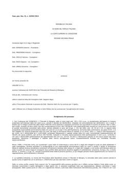
LATIFUNDIA REVISITED: MARKET POWER, LAND INEQUALITY AND
AGRICULTURAL EFFICIENCY. EVIDENCE FROM INTERWAR ITALIAN
AGRICULTURE*.
PABLO MARTINELLI
Department of Social Sciences
Universidad Carlos III de Madrid
E-mail: [email protected]
Abstract
This paper proposes a new interpretation of the historically controversial role of Italian latifundia.
Relying on standard economic theory, the paper explores a simple though neglected mechanism
linking land inequality and inefficiency: market power. In underdeveloped economies with serious
constraints on labour mobility, high ownership concentration will endow landowners with market
power in local labour markets. The resulting equilibrium explains many of the often criticised
features of latifundia, without the need to factor in irrational behaviour (the preferred explanation of
Italian traditional historians) or social institutions and capital market imperfections (explanations
advanced by economists in different contexts). According to the model here explored the main
effects of inequality are of a distributive rather than of a productive nature. The market power
hypothesis is strongly supported by the available quantitative evidence provided by an unexploited
dataset on all local labour markets of Italy at the end of the 1930s.
JEL codes: J42, J43, N54, O13, Q15
Keywords: Monopsony, Agricultural labour markets, Land distribution, Inequality, Italy
*
Acknowledgements. I would like to thank Giovanni Federico for his criticisms and suggestions, as well as seminar
participants at the European University Institute (Florence), Universitat Autònoma de Barcelona (UAB) and London
School of Economics (LSE), participants at the FRESH Meeting at the Universidad Carlos III (Madrid), at the First
Quantitative Agricultural and Natural Resources History Conference (Agricliometrics), at University of Zaragoza and at
the Ninth European Historical Economics Society Conference (held in Dublin) for their comments. Remaining errors
and interpretations are solely my responsibility. Support is acknowledged from the Spanish Ministry of Science and
Innovation project HAR2010-20684-C02-01.
1
1. INTRODUCTION
From Rome in times of the Gracchi brothers to contemporary Brazil and from postrevolutionary Russia to U.S.-occupied South Korea, land distribution has been a politically hot
topic throughout time and space. It was probably the main political source of domestic conflict in
agrarian societies, and also the most obvious one. Given its huge social, historical and economic
relevance, it comes as no great surprise that the issue from time to time has attracted the attention of
social scientists. In recent decades, economists in particular have increasingly regarded land
inequality as a key factor in the shaping of the development process, without reaching a consensus
on why exactly it matters.
One approach is to focus on the impact of land inequality on the efficiency of the
agricultural sector. These studies generally stress a combination of farm size with some sort of
market failure as a source of inefficiency. This literature can be summarized in two points: firstly, if
there are imperfections in capital markets, farmers may be unable to adjust to the optimal
operational size; and secondly, if labour markets are incomplete, labour may fail to be optimally
allocated across farms. Although different combinations of these market failures are claimed
(Barrett et al. 2010, Carter, 1984 and 2000, and Feder, 1985) to be the primary cause of the socalled inverse size-productivity relationship (ISPR), there is no consensus on the existence of the
ISPR itself. Other authors (Benjamin, 1995, Lamb 2003) claim that if one controls for land quality,
the ISPR significance disappears. In general, the empirical evidence is mixed1. Paradoxically,
despite the lack of conclusive evidence on the existence of the ISPR itself, there seems to be
evidence of a relationship between aggregate inequality and aggregate efficiency. Vollrath (2007)
finds a negative relationship between land inequality and agricultural productivity at the national
level; according to his estimates, market imperfections (and therefore resource misallocations) may
also account for most of the productivity differences between agricultural productivity in developed
and developing countries.
Other approaches consider the negative effects of land inequality on long run growth
through channels other than efficiency in agriculture. Deininger and Squire (1998), using the
available (but qualitatively limited) data from the FAO's international agricultural census databases,
find a negative relationship between land inequality and growth. The most recurring arguments in
explaining this relationship stress the political economy channel. Land inequality is said to create
strong incentives for some agents (generally but not exclusively the landed elite) to distort optimal
policy paths. Nonetheless, the exact mechanism through which land inequality works is again
1
See a review in Federico (2005) and, for the prosecution of the debate, Barrett et al. (2010) itself.
2
unclear. The factors proposed include: excessive, which is to say redistributive and growthinhibiting, taxation (Alesina and Rodrik, 1994, Persson and Tabellini, 1994); insufficient taxation
leading to the under-provision of public goods as education (Galor, Moav and Vollrath, 2009); trade
policy protecting rent extraction in agriculture (Adamopoulos, 2008); individual underinvestment in
education as a consequence of capital market imperfections (Deininger and Squire, 1998); and
extractive institutions (Acemoglu and Robinson, 2002 and Engermann and Sokoloff, 2000, both
with a very long run perspective). Although in some cases these incentives are clearly defined and
micro-founded, in others they are expressed rather vaguely; this is the case of “extractive
institutions”, which have become a sort of social scientists’ black box.
Yet, in all the previous explanations land inequality has at best an indirect effect. It matters
only if something else, combined with or caused by land inequality, prevents markets from working
properly. In this paper I show that land inequality can be itself a direct source of inefficiency. It is
not only the case that a concurrent element (either capital markets or institutions) matching some
variable correlated with land inequality (either the concentration of elite’s power or the dispersion
of farm sizes form the optimal operational size) leads to suboptimal equilibriums in competitive
markets. It is excessive landownership concentration itself that may prevent markets from being
competitive.
This paper shows that land inequality is one of such cases where the most straightforward
explanation is simply not on the market while a simple and almost textbook one can do the job,
provided a complete enough dataset is available for implementing a suitable and testable strategy.
Rather than focusing on frictions to farm size adjustment or extra-economic factors and institutions,
the core mechanism exposed in this paper is that a high degree of landownership concentration, on
its own, endows landowners with market power in poorly integrated rural labour markets.
The basic intuition is that, in agrarian economies with positive costs of factor mobility, the
most concentrated landownership is among landowners, the more relevant economic agents the few
landlords at the top of the land distribution are, and the more impact on local markets their
economic decisions have. Hence, the most unequal the distribution of a non-reproducible asset like
land is, the more the resulting equilibrium departs from the competitive case. In such cases,
landowners will have an incentive to demand less labour than those in competitive markets, as a
standard monopsony model predicts. Productive inefficiency will emerge in such an economy. In a
general equilibrium approach aggregate welfare losses will be relatively reduced, as foregone
employment in the dominant estates will be partially compensated for by increased employment in
the non-agricultural sector or in price-taking farms. Nonetheless, the economy will be characterized
by strong distributive distortions. Factor allocation among sectors will be suboptimal and there will
3
be strong incentives for the landed elite to block the development of the non-agricultural sector and
to raise further barriers to labour mobility.
Conversely, in a competitive economy, landowners are price-taking, and thus their
productive decisions have no impact on relative factor prices. Asset distribution within one class of
factor owners shall not affect income distribution between different classes of factor owners. These
facts will provide a clear guidance to test the theory.
The simple mechanism explored in this paper is independent of and yet easily relatable to
almost any channel already proposed. Moreover it is unambiguously testable, provided the required
data is available. Beyond an obvious connection with the political economy channel, the stress on
landownership concentration itself as a source of inefficiencies may account at once for the disputed
empirical evidence on the ISPR and for the stronger evidence on a negative correlation between
inequality and aggregate output. Yet, the focus shift from farms to actual ownership poses
formidable measurement problems, which may partly explain why market power has been so far
neglected by the literature on land inequality. Being direct and simple does not imply being easy to
be empirically verified. Thanks to an unusually detailed database (used here for the first time in
scholarly research), the hypothesis can be tested by addressing the unsettled question of latifundia
in Italian pre-WWII agriculture.
The Italian interwar agriculture constitutes an exceptional field for testing the hypothesis.
Politically, land distribution was a highly controversial issue and a source of rural distress until the
land reform implemented after World War II. Scholarly work reflected this controversy. Traditional
historiography considered Southern latifundia in a very negative manner. Modern economic history
has successfully (and convincingly) criticized the traditional view, which essentially assumed that
landowners behaved irrationally. However, modern economic historians have failed to explain the
widespread discontent with the issue in the late nineteenth and early twentieth century. A dismissive
approach is also inconsistent with economists’ increasing concerns about the role of land inequality.
Relying on a market power model, this paper explains many of the features of Italian latifundia by
the simple use of economic theory and assuming the rational behaviour of agents. Contrary to the
traditional Italian historiography, land inequality is not seen as a source of technical inefficiency in
agricultural production, but caused important distributive distortions through factor misallocation
among sectors. Reduced wages, reduced aggregate output, extensive technical mixes (but not lower
TFP), agricultural underemployment and Pigouvian exploitation arise as an equilibrium from the
model without the need to introduce restrictive assumptions on agents’ behaviour. Whether land
reform is the best means of addressing these issues as against other forms of fostering labour market
integration remains an open question, which this paper does not set out to address.
4
Hence, in this paper I present and test a new, simple, purely economic and so far neglected
explanation for latifundia’s inefficiency. A simple neo-classical model of market power and
Pigouvian exploitation suffices in illustrating the economic basis of the conflicts arising from
landownership concentration. While economic development, reduction in information and transport
costs, and market integration are likely to erode local market power positions, barriers to and costs
of factor mobility were much higher in the past, and may still be considerably high in areas weakly
affected by world economic integration or where authorities deliberately restrict free movements of
capital and labour. The local market power model thus seems particularly suited to historical
analysis.
The paper proceeds as follows. In Section 2 I present the historical controversies that
surrounded Italian latifundia and explain why the particular Italian case at the end of the 1930s is a
proper field to test the theory. In Section 3 I briefly present a stylized two-sector closed economy
model, which provides two different testable equations for the market power hypothesis and
describes the main features of the case. Section 4 presents the main data and sources used. Land
inequality measurement is also discussed. Specifically, I discuss several empirical problems usually
neglected by literature and I present an exceptional database, used here for the first time, on land
inequality in Italy around the late 30s and early 40s, which is not affected by these problems.
Finally, the results of the benchmark regressions and several robustness checks are presented and
discussed in Section 5. Section 6 concludes.
2. LAND INEQUALITY AND THE ITALIAN ECONOMY BEFORE WWII
Land inequality has traditionally been an issue which has stoked political controversy in
Italy. Its origins can be traced back to the end of the ninetieth century. Latifundia, as the large
estates (mainly in Southern Italy) were called, were often at the centre of political projects to
improve the conditions of the Southern economy, ranging from state-built roads and irrigation
infrastructure to compulsory renting out of estates2. These projects were constantly a topic of debate
in Italian politics during the first half of the twentieth century, but none of them were significantly
implemented. The emergence of unionism and workers’ political organizations at the turn of the
century led to a qualitative shift in the public debate (Zaninelli, 1971). Workers’ demands usually
went beyond wage increases. According to a parliamentary inquiry on the conditions of Southern
2
See Lupo (1990) for a summary of the controversies at the end of the XIXth century and Molé (1929) for the
persistence over time of many of such analysis and seldom realized proposals.
5
peasantry (Inchiesta Faina 1909), in latifundia areas the main concern of rural labourers was
seasonal and chronic unemployment, attributed to excessively extensive agriculture. Thus, one of
the main aims of workers’ agitations during this period was to impose on landowners a minimum
level of yearly employment (the so-called imponibile di mano d’opera). After WWI the level of
social conflict in the countryside dramatically increased, and there was a widespread occupation of
allegedly idle land in many latifundia during the revolutionary upsurge of 1919-1921. That
movement was brought to a violent end with the rise of Fascism in October 1922. In 1935, a project
for making compulsory agricultural intensification in some latifundia areas was so strongly and
successfully contested by large landowners that its reversion caused the political fall of its foremost
proponent, the government official for the so-called “integral land-reclamation” Arrigo Serpieri
(Orlando, 1984). As soon as WWII ended, social conflict in the countryside, strikes and land
occupations resumed, until eventually a selective form of land reform took place at the end of the
1940s and the beginning of the 1950s.
Italian traditional historiography reflected the controversy surrounding the historical role of
land inequality, but it has nonetheless failed to provide a coherent interpretative benchmark
grounded in economic concepts and has seldom integrated quantitative evidence into the discussion.
The conventional wisdom was stated in its clearest form in the seminal work of the Marxist scholar
Emilio Sereni (1977 [1947]). He attributed a central role in the Post-Unitary Italian growth story to
large Southern estates. Their landowners’ absenteeism was at the root of the chronic
underemployment of the labour force in the countryside, the low productivity of the latifundia
agriculture, and the failure to introduce new crops or new productive techniques. The short-term
rent contracts prevented tenants from investing in land improvements. “Pre-capitalistic” and
“feudal” survivals pervaded contractual agreements and characterised agents' behaviour. The
persistence of sharecropping agreements also reflected the low degree of capitalist development in
the Italian countryside (Sereni, 1977 and Giorgetti, 1974 and 1977). Collectively, these factors
precluded the introduction of new kinds of rotations allowing for the expansion of livestock and the
implementation of mixed husbandry as had been done in North-Western European countries. Only
the capitalist farming of the Po Valley was considered “modern” and “advanced”, but it was not
sufficiently widespread to boost modern economic growth across the country. As a consequence,
both agricultural production and agricultural productivity languished, and in turn this damaged
industrial growth. Agriculture was thus at the core of both the enduring Italian regional divide and
the slow growth rate of the Italian economy prior to the “economic miracle” (1951-1963). In
successive years, non-Marxist scholars have stressed that there were further reasons behind
6
Southern Italy’s backwardness, but the negative interpretation on the role of latifundia and Southern
landowners has persisted over time (Toniolo, 1980, and Zamagni, 1993).
In recent decades, a revisionist body of literature on these picture has emerged. First, large
landowners’ behaviour has been radically reconsidered. Some case studies (Petrusewicz, 1989,
Placanica, 1990) stress that, regardless of their social origin (aristocratic or bourgeois), they were
acting as profit-maximizing and rational economic agents, especially if one considers that the
environmental conditions typical to Southern Italy, for example the lack of rain in summer, largely
preclude the implementation of the Po Valley crop mixes (Lupo, 1990, Bevilacqua 1990). Many
contractual agreements - once negatively considered by literature - are now seen as satisfactory
solutions to specific risk-bearing problems (Cohen and Galassi, 1990 and Galassi and Cohen,
1994)3. Secondly, the important quantitative reconstruction of the Italian historical national
accounts has substantially shaped scholars’ view of Italy’s growth4. This revision corrected the
myriad shortcomings of the traditional ISTAT-Fuà estimate (Fuà, 1975 [1969]) but also provided
the basis for national accounts estimates at the regional level in historical perspective, at least for
some branches in some benchmark years, thus providing the only serious ground for any discussion
on the matter. The main results are as follows: overall GDP growth was somewhat more satisfactory
in the fifty post-Unity years than was previously thought (especially thanks to agriculture); there
were noticeable, although not radical, differences in industrialization levels between North and
South as a whole at the time of Unification (and in the few decades following 1861); agricultural
labour productivity was similar (with some Southern regions performing particularly well) until
WWI and only started diverging in the interwar years. As differential rates of agricultural TFP
growth are likely to have caused this divergence in the agricultural branch (Federico, 2007),
determinants of efficiency in agriculture are worth exploring. As a consequence, the GDP
divergence between the Northern and the Southern sections of the country is now considered much
more of an issue in the first half of the XXth century than in the XIXth, and it is due at least as much
to agriculture as to industry.
Three elements emerge from these developments. Firstly, land inequality has lost its central
role in contemporary Italian history. We no longer see latifundia as feudal residuals causing the
Italian regional divide, but, after the loss of its predominant position in the discourse, land
inequality is searching for its place in Italian economic history. Secondly, we have to accommodate
this story with the fact that many early twentieth century Italians (observers, politicians,
3
See Cohen and Federico (2001) for a full account of the new trends of the history of Italian agriculture in general and
of this brand of revisionist literature in particular.
4
See Rey (ed.), 1992 and 2000, and different spillovers as Federico, 2003a, 2003b and 2007, Felice, 2005 and Felice,
2011, Ciccarelli and Fenoaltea, 2010).
7
intellectuals and, above all, rural labourers) were really concerned with land inequality (as many
present-day economists are) - so concerned in fact, that a land reform was eventually implemented
after WWII. Thirdly, the interwar years seem to deserve special attention, much more than previous
research, which mainly focused on the 1861-1911 period, has paid. Whatever role land inequality
played in Italian agriculture, it is likely that its effects peaked between the wars. Addressing such
questions may require that we avoid the approach of traditional historians, i.e. to look for ad hoc
sociological or psychological explanations about landowners' absenteeism or about their propensity
to engage in market transactions.
In this context, the market power hypothesis, fully-rooted in economic theory, may help to
fill this gap in Italian economic history. Moreover, beyond the desirable property of data
availability, there are reasons for considering the Italian economy at the end of the 1930s as a
proper field in which to test the market power hypothesis. The Italian economy was, at that time, a
semi-industrialized one. Agriculture still employed 52% of the labour force according to the
Population Census of 1936. Despite the fact that a slow process of industrialization had begun some
decades earlier and the building of a railroad network had already been completed by the beginning
of the twentieth century, the modern sector was mainly confined to few industrial cities in the
North-Western part of the country - the so-called industrial triangle with vertices at Milan, Turin
and Genoa. In addition to Italy largely qualifying as a developing country before WWII, the country
possessed some specific characteristics that are likely to have enhanced landowners’ market power.
Free unionism had been banned in the 1920s by the Fascist dictatorship, and the bargaining power
of landowners was consequently enhanced (Cohen, 1976). Industry was severely hit by the crisis,
and thus its role as a potential alternative occupation was strongly affected. Industrial employment
fell by 22% between 1929 and 1932, and the pre-crisis occupational peak, 1926, was reached again
only in 1937 (Zamagni, 1976). The Great Depression and US’s restrictive post-WWI immigration
policy effectively blocked emigration as an alternative. Gross international migration fell to close to
the historical minimum of the WWI years and net migration was actually negative in the late 1930s
(ISTAT, 1958). Railroad movement of passengers remained stable throughout the 1920s and 30s
(ISTAT, 1968). Mass motorization had not yet started, and where communication was concerned,
many latifundia areas were poorly connected with the rest of the country (Molè, 1929). Land
inequality may itself be a barrier to migration in a context of diffused rural poverty and credit
constraints. Aside from the economic and structural features of the Italian economy, starting in
19285 the Fascist regime implemented allegedly “ruralist” policies and tried to push people to the
5
The Law n. 2961 of December 24th 1928 enabled provincial prefects to issue ordinances in order to “limit the
excessive growth of urban population”. These ordinances typically took the form of banning migration to the most
8
countryside6, trying to avoid free internal migrations and “urbanism”. Along with other minor
regulations enacted during the 1930s, migration from one province to another in search of an
occupation required official authorization (Law n. 358 of April the 6th 1931, which instituted the
Commissariato per le migrazioni e la colonizzazione interna) and migration to municipalities of
more than 25,000 inhabitants was virtually prohibited (Law n. 1092 of July the 6th 1939,
Provvedimenti contro l’urbanesimo).
Thus, the institutional and economic shock to which the Italian economy was subjected in
the interwar years constitutes an ideal environment that allows testing whether land ownership
inequality leads to market power in the context of low mobility of labour and weakly integrated
internal labour markets or not. This approach, moreover, will help to shed light on the role played
by land inequality in Italian development during this period, an issue so keenly debated by Italian
historians.
3. ANALYTICAL FRAMEWORK: LAND INEQUALITY AND MARKET POWER
This section introduces an analytical benchmark to cope with land inequality and market
power, and outlines a feasible empirical strategy by deriving from that benchmark two equations
testable with the available data.
As noted in the introduction, the main hypothesis to be tested here is that, if factor markets
are relatively local, a high concentration of land ownership may endow landowners with market
power. This means that as a consequence of landowners being relevant agents in factor markets,
factor prices will be affected by their factor demand and supply decisions. The main features
characterizing such a situation can be illustrated by a simple model of monopsony in the labour
market. This is admittedly the extreme case of market power; far from being a common situation, it
constitutes the upper bound to which extreme land inequality can tend. Perfect competition is the
lower bound. For analytical purposes, comparing the two extremes will prove useful.
Let us start with a very stylized two-sector economy. Sector A is agriculture and sector B is
non-agriculture. Assume each sector has a simple Cobb-Douglas production function with a single
output and let us consider the relative output prices exogenously fixed by international trade and
normalized to 1.
important cities of the province to people without an employment. Prefects largely made use of these powers: by
December 1931 67,4% of them had some ordinance issued (ISTAT, 1934).
6
See Treves (1976). Despite the fact that the effectiveness of such policies may have been mixed, it substantially
increased the cost of internal migration and was deemed as “a sort of new feudalism” by the leading liberal economist
(and later president of the Italian Republic) Luigi Einaudi.
9
YA and YB are, respectively, the output levels of the agricultural and non-agricultural sectors. EA and
EB measure technology and other scaling factors, such as environment in the case of agriculture. TA
is the total amount of land in the economy, totally devoted to agricultural production. LA and LB are
the labour inputs allocated in the agricultural and in the non-agricultural sector respectively. KA and
KB are the capital inputs (considered fixed and sector-specific) in agriculture and in non-agriculture.
The total endowment of each factor is exogenously given. In competitive equilibrium, agents
maximize output and the full use of resources is granted. Workers can move freely between
agriculture and non-agriculture, and the same wage rate w is paid in the two sectors. The
competitive equilibrium solution to such a system is given by the standard first order equations that
maximize profits in the two sectors and by the factor markets clearing conditions.
In the standard framework of monopsony in the labour market, a single landowner owns all
the land in the economy. Thus he is the single employer in agriculture and is a relevant employer in
the whole economy. As a consequence, he faces the maximization problem in which the wage rate
represents the inverse labour supply to agriculture; i.e. the landowner faces the problem of
maximizing YA-RTA-w(LA)LA-rKA with respect to TA, LA and KA (where R, w(LA) and r are
respectively unitary rent, wage and capital return rates).
The usual first order conditions, together with the market clearing ones, define the
equilibrium in this economy. The demand for agricultural labour is implicitly given by:
where ε = (∂LA/LA)/(∂w/w)>0 is the elasticity of the labour supply curve with respect to wage. The
labour supply to agriculture is LAS = L-LBD = g(w). At any given wage rate, the amount of labour
supplied to agriculture is what is left after the non-agricultural demand for labour (given by the
marginal product of labour in non-agriculture) is deducted from the total stock of labour. The
resulting equilibrium is obviously inefficient because marginal product of labour does not equalise
among sectors, as (∂FB/∂LB) = w but (∂FA/∂LA)[ε/(1+ε)] = w. The landowner demands less labour
than he would in the competitive case and the remaining labour is absorbed by the competitive (i.e.
wage-taking) non-agricultural sector. Despite the fact that agricultural output is therefore reduced,
10
non-agriculture produces more output than it would in the competitive case. This means that, in a
general equilibrium approach, aggregate welfare losses are smaller than a partial equilibrium
analysis would suggest, but the distributive effects among factor owners as well as factor allocation
among sectors are relevant. The whole situation can be seen graphically in Graph 1, where the
superscript “C” and “M” denote the competitive and monopsonistic cases respectively.
It is not only the aggregate output which is lower than in the competitive case. Perhaps more
interestingly, the agricultural labour to land ratio (the degree of intensity of agriculture) is lower in
the presence of landowners’ market power than it would be in the competitive case. Equilibrium
wages are lower, and aggregate welfare is also lower due to deadweight losses. Landowners are
better off than in the competitive case, but now workers in both the agricultural and non-agricultural
sectors earn lower wages7.
7
In order to properly interpret this result, consider that the non-agricultural sector can be thought of as an aggregate
sector, which includes not only industry but also services and domestic occupations. We can think of the labour supply
curve to agriculture as the subtraction form the total endowment of labour of the horizontal sum of the demand curves
for all activities other than agriculture. Those activities with higher marginal products of labour at a null level of
employment appear in the upper side of the curve and will be the first sectors to which labour in non-agriculture is
allocated, and so on. Thus, employment in non-agriculture at low levels of wages goes to activities with low MPLs and,
thus, with low social opportunity costs. In this sense, the labour supply to agriculture can also be thought of as capturing
the reservation wage of workers. In any case, the activities that compensate the reduced agricultural employment have
lower marginal products of labour than the competitive ones in both agriculture and non-agriculture, implying a shift
towards activities with lower opportunity costs and losses of aggregate welfare.
11
GRAPH I: LABOUR MARKETS IN A 2-SECTOR ECONOMY. MONOPSONY AND
COMPETITION.
These patterns explain many features of the latifundia economy often criticised by
observers, summarized in Table 1. The resulting equilibrium arises from the rational and optimal
choices of both landowners and workers. Given the existing asset distribution, the equilibrium is
also a result of workers' free choice, so no reductive assumptions on forced labour or similar are
necessary. One can think of the non-agriculture sector as also including a competitive fraction of
agriculture (i.e. price-taking farm operators), without substantially altering the results.
12
Table 1: Monopsony explaining latifundia’s features
Competition (C)
Traditional
latifundia’s features
vs
Monpsony (M):
Explanation of Market Power Effects
Comparison of
Equilibria
“Extensive agriculture”
“Widespread rural
poverty”
LAC/T>LAM/T
wC>wM
“Chronic
underemployment in
Reduced labour demand per unit of land results in either extensive
crop mixes or non-labour intensive technical mixes.
Equilibrium wages are reduced in the whole economy (i.e., both in
the agricultural and non-agricultural sector).
Labour employment over the year for agricultural activities is
C
LA >LA
M
reduced.
agriculture”
“Exploitation”
MPLAM> wM
“Chronic
underemployment in
agriculture (bis)”
The gap between MPL in agriculture and wages implies Pigouvian
exploitation.
Depressed wages and employment in agriculture increases the size
LBM>LBC
of low-opportunity cost sectors (either employment in sectors with
lower MPL than the competitive one or inactivity and domestic
activities).
“Underdevelopment”
YC/ LC> YM/ LM
Aggregate GDP per capita is reduced because of deadweight
losses.
Landowners are thus able to extract rents from the system (as implied by the underlying
reasoning in Acemoglu and Robinson, 2002) and they have strong incentives to obstruct the upward
shift in the labour demand curve of the non-agriculture sector, whether through the manipulation of
trade policies (as suggested in Adamopoulos, 2008), or a reduction of the investment in public
physical capital (Banerjee and Iyer, 2005) or public human capital (Engerman and Sokoloff, 2000
and Galor et al., 2009, among others). The rent-extraction activity may determine various forms of
self-enforcement through the political process or may be determinant in shaping institutions.
Nevertheless, these outcomes are not necessary, as inefficiencies arise directly from market
equilibrium. Moreover, a situation like the one described by this model is more unstable in
democracies than in dictatorships. In democracies, majorities are likely to remove obstacles to
factor mobility and accumulation in the competitive sector or even asset redistribution in the event
that welfare losses for the majority are huge and evident, though such an outcome is by no means to
be taken for granted. This prediction is also consistent with the results found by Deininger and
Squire (1998).
13
A reasonable procedure to test the theory would be to take as many local labour markets as
possible and observe if higher concentration of land ownership leads to a systematic departure from
the competitive case towards the monopsonistic case. But these departures need to be expressed in
at least one testable equation which can be confronted with hard data. In the empirical strategy that I
follow, the model is double-checked against the available quantitative evidence. Rather than merely
testing alternative specifications of the same theoretical equation, two different testable equations
are independently derived from the same theoretical model.
As far as we observe w and LA, we do not know if such values are due to market
inefficiencies or to different MPLs (caused by different stocks of the other factors or by differences
in the environmental-technological scalar EA). Demand for agricultural labour depends on the total
amount of capital and land, as well as on the sector-specific technical coefficients. Thus, it is not
possible to unambiguously estimate (3), as any estimate will always be suspected to be subject to
omitted variables bias (as is the case with the ISPR).
To avoid this kind of problems, the first testable equation is obtained in the following way.
Consider that another of the first order conditions (in both the competitive and in the monopsonistic
cases), namely the identity between the marginal product of land and its price (the unitary rent), is:
Dividing (4) by (3) allows cancelling both KA and EA, and hence one gets:
The analogous expression for the competitive case is:
Equations (5) and (6) are much more tractable than the general solutions to the foregone
systems (and require much less data). Their interpretation is straightforward: in equilibrium, relative
factor prices are inversely proportional to relative factor intensities. In the case of one sectorspecific factor, as is the case of land for agriculture, this is even simpler, since relative prices are
expressed in terms of the ratio of agricultural employment to the whole land endowment. Under
14
monopsony, relative prices are systematically shifted against the “monopsonized” factor. Taking
logarithms of both sides of (5) and (6) yields:
Now, when ε→∞, ln[(1+ε)/ε]→0 and (7)→(8). Conversely, when ε→0, ln[(1+ε)/ε]→∞.
When landowners lose market power, the equilibrium solution tends to the competitive case. In this
sense, (8) can be interpreted as a particular case of (7). ln[(1+ε)/ε] is a positive term which grows
monotonically according to the degree of landowners’ market power.
Note that the expressions (7) and (8), as they are expressed in terms of relative prices and
factor endowments, are independent of the endowments and prices of the other factors, particularly
environment and capital in agriculture. In particular, if markets are competitive and the production
function is Cobb-Douglas, (8) is always true irrespective of the amount of capital and the level of
technology in any sector. In (7) capital and technology in non-agriculture enters the expression
through ε: if there is a systematic departure from relative prices due to market power, they have an
effect on the size of the departure. Admittedly, (7) and (8) are two limit cases, in which perfect
competition and a single landowner operate, respectively. Other employers can be introduced into
the market, allowing for more complex interaction: for example, considering a model in which the
largest landowners operate as a leader cartel and another set of wage-taker followers exists.
Nonetheless, all of these cases lie somewhere in between (7) and (8). What matters here is that if
land ownership concentration endows landowners with some degree of market power (i.e. their
actions have some impact on market prices), an increase in land ownership concentration will
systematically result in a shift of relative factor prices away from their competitive ratio
(determined by factor intensity). That is to say there will be a move from the competitive case (8) to
the monopsonistic case (7). The point is not so much the magnitude of the shift, but its systematic
association with increasing land ownership concentrations.
One may reasonably think that a high concentration of land ownership may endow
landowners with market power in the labour market as well as in the land market. Monopoly in land
markets would cause rents to be higher than in a competitive environment (in a symmetric way with
respect to the outcome in the monopsonistic labour market), so the rent-wage equilibrium ratio
would be shifted upwards, strengthening the effect of monopsony in the labour market. Adding this
situation would complicate the model without substantially altering its qualitative predictions.
15
Defining a testable equation in relative rather than in absolute terms is indeed a way to capture any
shift in relative factor prices caused by market power, irrespective of whether it is exercised in some
cases in the labour market and in others in the land rental market. As far as the main aim of this
paper is to verify if land inequality leads to some degree of market power, it is irrelevant here
whether it is exercised in labour markets, land markets or a combination of the two. However,
Carmona and Rosés (2012) find land markets working rather efficiently in Spain during the first
third of the twentieth century, a finding that justifies to focus mainly on the functioning of labour
markets8.
Hence, in order to investigate whether land inequality actually leads (8) towards (7), we can
rely on the testable equation (9):
In (9), C is a measure of land ownership concentration (with a 0 lower bound), X’ a vector
of control variables and u an i.i.d. error term. In a competitive economy, there is no reason for one
factor ownership concentration to shift relative factor prices. Thus, testing whether b2=0 in (9)
allows us to discriminate between the competitive (8) and the market power (7) cases, and hence
assess whether land inequality is cause of inefficiencies itself. Moreover, it also seems to be the
most interesting factor to test, because as we have seen the more relevant consequences of market
power are on distribution rather than on aggregate output levels.
But two checks are better than one. From the first order conditions for the agricultural sector
we can derive a second equation, one in which absolute prices are now stated in terms of average
output per worker. In particular, it is worth noting that the monopsonistic and competitive cases are
respectively (3) and:
Again, it is standard to see that expression (3) collapses to (10) as ε → ∞. Taking logarithms
and rearranging, we obtain:
8
Focusing on labour markets is also justified by the fact that in 1936 rented tenants were just 9% of the Italian
agricultural labour force.
16
Hence, there is a linear relationship between the average output per worker in the
agricultural sector and the equilibrium wage, as stated in (10). This means that, in the presence of
market power, land inequality causes a gap between the average product of labour and the ongoing
wage rate. The simple intuition behind such a result is that, with diminishing returns to labour and
in the presence of monopsony, landowners will stop hiring labour before marginal productivity
equals the ongoing wage rate. While in competition marginal productivities (and hence a given
fraction of partial labour productivities) equalise wages, in monopsony the former is always greater
than the latter. If land inequality endows landowners with market power, the gap between partial
productivity and the wage rate will increase as landownership becomes more concentrated.
Allowing for the same set of controls considered in the previous section, the second testable
equation can be defined as:
Whatever specification of the testable equation we consider, what it is worth noting here is
that a different equation involving partially different variables has been derived from the same
model. While in regard to the first equation the research strategy is to test the effect of land
inequality on shifts of relative prices given relative factor endowments, in regard to the second it is
possible to test its effects on deviations of the absolute price of one factor (labour) from its average
output. Finding statistical evidence for two different (though interrelated) predictions arising from
the same theoretical model certainly strengthens the validity of the model itself as a representation
of reality.
4. DATA: A NEW DATASET ON INTERWAR ITALIAN AGRICULTURE.
Estimating (9) and (12) is possible only if data on all the involved variables for as many
local labour markets as possible are available. It is evident how stringent this requirement is, in
particular when considering the need of a measure of land inequality that properly measures
landlords’ market power. Fortunately, there exists an almost unique dataset for late 1930s Italian
agriculture that allows us to test such equations, taking a cross section of all local rural labour
markets of Italy. In this section I describe the main sources and methods used to obtain the required
variables.
17
Data on land inequality come from a post-WWII official inquiry in which information about
every single owner all over the country was collected with such a detail and satisfying so high
quality standards that the inquiry has remained unmatched by any other national dataset on land
inequality ever since. Given the importance of the topic, I start with it.
4.1. A new high-quality database on land inequality for Italy, 1940 ca.
For a dataset to be considered truly representative of the actual landownership concentration
as it is required in this study, some rarely matched quality standards are a prerequisite:
(I)
Data must be based on sources with full coverage of the economy under study such
as a Census or an inquiry carried out with similar procedures and coverage, avoiding
both unrepresentative sampling and imputation procedures out of national account
systems.
(II)
Data must yield information on actual ownership distribution, not farms, operational
units or tax-payment distributions.
(III)
Because land is not a fungible good, data must refer to the distribution of the
economic value of land or at the very least must include data that may enable an
adjustment.
(IV)
Data must specify whether a property is individually or collectively owned, as may
be the case under communal tenure arrangements.
While these requirements seem to be rather obvious, they are usually neglected by the
literature on land inequality. These reasons may help to explain why market power in rural
economies as a source of inefficiency has rarely been addressed - quite simply, it is too difficult to
measure.
For the purposes of this paper, I rely on an extraordinary database that adequately matches
all the standard requirements to fully qualify as a proper database on land inequality. This is also the
first time that such a database has been employed in research. The source of the database is a
massive national inquiry carried out by the Italian government in the immediate aftermath of WWII.
The government entrusted the INEA (National Institute of Agrarian Economy, a public agency
dependent on the Ministry of Agriculture) to carry out the inquiry, which it did between 1945 and
1946. Although officially it was just an informative inquiry, such a statistical effort is thought to
have been a part of the preparing process of an upcoming Land Reform (the Minister of Agriculture
was then a Communist). Data collected by the INEA inquiry was published between 1946 and 1948
18
in 13 regional volumes, with the name of La distribuzione della proprietá fondiaria in Italia (“Land
ownership distribution in Italy”). Information was collected about the ownership of every single
plot in the country (with few spatial gaps), its size and rent, and the institutional characteristics of
the owner - whether he was an individual, a public entity, a charitable organization, etc. Data were
gathered from Cadastral registers in every municipality, where all plots of the municipality were
assigned to a landowner. Land rents had recently been estimated for fiscal purposes and included in
the tax-payer register (see below on this point). These data match standard (I). With these data,
inquirers proceeded to cumulate all the plots owned by the same owner (whether an individual or an
organization) in order to ascertain each owner’s actual ownership within the municipality. Two
different distributions of ownership at municipality level were published: one classifying
ownerships by size, the other by rents. The accumulation was also done at agrarian zone level9, then
at agrarian region level (groups of agrarian zones within each province), at provincial level, at
regional level and at Italy-wide level. This makes the data matching quality standard (II). Moreover,
for each agrarian zone the inquiry also published separated distributions for personal private
ownerships and “entities” ownerships, which included mainly public or semi-public lands. Hence,
for this level of aggregation10, standard (IV) is also matched.
Finally, it is worth a word on rents and on matching of standard (III). There is obviously a
difference between economic rent and legal rent. If rents are considered as the economic return to
land (rather than as actual payments made by tenants), they capture their marginal contribution to
production, i.e. its marginal value. In this sense of the word “rent”, every plot yields a rent,
irrespective of its tenure arrangement. Thus, the distribution of rent so understood is equivalent to
the distribution of productive value-adjusted land. Fortunately, for the purposes of this paper, the
rent that was registered for tax purposes and that the inquiry collected was the economic, not the
legal rent. A few years before, those rents had been estimated simultaneously with uniform, rational
and up-to-day accepted criteria for the first time. In 1939 the fascist regime managed a general and
simultaneous revision of the Cadastre in order to increase the tax revenue to fund the coming war
effort. New and uniform assessment criteria were introduced, which more rigorously reflected the
economic rent (they were, indeed, the definitive criteria which have been in force ever since). The
rent had to be valued as the actual contribution of land to production, thus discounting actual labour
inputs (irrespective of their contractual arrangements), intermediate inputs and capital inputs
9
The Agrarian Zone was a very disaggregated statistical unit introduced in 1909 by the statistical service of the
Ministry of Agriculture in order to carry out the first Agrarian Cadastre (a national survey of agricultural production,
which was only partially published). It was formed by municipalities of homogeneous agronomic and economic
characteristics. Their number grew with time, and in 1945 Italy was divided in 775 Agrarian Zones. In this paper they
are the basic unit of observation.
10
The agrarian zone is in any case a rather low level of aggregation: the average area of an agrarian zone was 143
square miles, slightly more than one tenth of an average US county.
19
(including the amortization of fixed capital investments). The contribution of capital and the
operator managerial inputs had to be valued in a different taxable figure, which constituted the base
for a tax on the returns to agricultural capital. Input had to be considered at the actual local input
mixes, and output and input prices (including wages) had to be valued at local prices. Output and
prices taken into account had to be the average ones for the period 1937-1939. The re-estimation
was done relatively quickly, as the new tax-figures were put in force in 1943. For the first time in
Italian history, land rents were valued as the land shadow-price of land with proper agronomic and
economic criteria for almost the whole country (where the new Cadastre had been implemented)
with a uniform method and valued at prices referred to a close period. As a consequence, the only
period in the whole span of modern Italian history for which a national cross-section of land rents
from the land tax figures is fully reliable and available is precisely the years 1937 to1939.
This period is not very distant from that for which land distributions are available. In view of
the fact there is no evidence of significant changes in land distribution between 1939 and 1945 (the
land market seems rather to have frozen during the war11), I will consider the land distributions
reflected in the government’s inquiry as being fully representative of the 1937-1939 period.
Due to the published double distributions (of ownerships grouped by size and by rents), the
inquiry facilitates the estimation of a value-adjusted land distribution, thereby matching standard
(III) and overcoming the usual land quality heterogeneity problem as discussed in the inverse sizeproductivity literature. Summing up, such an impressive dataset enables the computation of
inequality indexes that may be very close to the actual concentration of demand for agricultural
labour. Gini and Theil indexes have been computed over several alternative distributions,
specifically private and/or public land distributions and size and/or value distributions. Despite its
popularity, the Gini index lacks certain properties which are regarded as desirable by scholars in the
measure of inequality12. Inequality among the wealthy seems to be more related to market power (as
the poor are not likely to demand much labour), and thus a measure yielding higher inequality
levels for Lorenz curves steeper at their end may be preferable. Decomposability can also be shown
to be desirable when considering alternative definitions of “local labour market”. This makes the
Theil index preferable to the Gini index for the purposes of this paper.
11
The number of land purchases, the only available index of activity in the land market, collapsed during WWII to the
historical minimum level of the whole series (starting in 1896), i.e. 119.000 in 1945, a level never seen before even
during WWI, when the population was more reduced and poorer (ISTAT, 1958). Never since 1918 had such a number
fallen from 200.000 purchases per year (though it was lower every single year from 1940 to 1945).
12
In particular, the Gini index is not always decomposable and does not satisfy the weak principle of transfers. See
Cowell (2009) for this point and for the following methodological issues regarding inequality measurement.
20
MAP I: VALUE-ADJUSTED LAND INEQUALITY (ECONOMIC RENT INEQUALITY).
ITALY, 1940 ca.
Theil Index
Private Properties
0.57 to 1.20
1.20 to 1.59
1.59 to 2.00
2.00 to 2.50
>2.50
No Data
Map 1 represents the computed Theil index of value-adjusted land inequality of private
ownerships, the preferred measure of market power. It shows the first mapping ever of Italian land
inequality in the first half of the XXth century. The unit of analysis is the agrarian zone, which
seems to be the optimal one for representing local labour markets (being larger than a single
municipality and smaller than a whole province). The overall picture shows high inequality in many
of the very same areas that after WWII witnessed the implementation of the land reform, with two
21
notable exceptions: the area of high landownership concentration in the western part of the Po
Valley (a rice-growing area), which was not affected by the land reform, and Sardinia, which was
affected despite not showing extreme levels of inequality. Many areas of Southern Italy display
generally high levels of landownership concentration, though the picture is more mixed than
assumed in traditional historiography: very low inequality can be found in Campania and along the
Tyrrhenian coast, in some areas of the central coast of Apulia and in the Abruzzi. In the area of
Central Italy spreading from Latium to Tuscany and Umbria it emerges another focus of high
landownership concentration. This feature has been so far neglected by traditional historical
accounts, probably because the diffusion in this areas of medium-scale sharecropping family
farming hid the actual degree of asset inequality13. Finally, the map suggests that land inequality
was strongly correlated with the electoral support at a local level to the Socialist and Communist
parties (the most decided advocates of a land reform) in the first elections after WWII.
4.2. Other data on Italian agriculture at the end of the 1930s.
From January 1938 the Bollettino Mensile di Statistica Agraria e Forestale (ISTAT, various
issues) published monthly wages of close to 200 agricultural wage zones into which the country had
been just divided. I assigned a wage to every single agrarian zone according to the wage zones’
boundaries (BMSAF, fascicles of January and February of 1938). In order to test equation (9),
wages and rents have to be comparable. Since unitary rents are measured as the returns to the land
input on a yearly base, wages must be measured similarly. I computed weighted annual wages for
men and women, taking into account differences in the number of hours worked across the year and
across the country (also published in the BMSAF at wage zone level) and the monthly changes in
wages14. Two different sets of wages have been computed: one making a simple average of men
and women’s wages (hereinafter referred to as “unweighted wages”) and the other weighting each
wage for the share of women within agricultural employment in the region (as appeared in the
census) to which the agrarian zone belonged to (hereinafter referred to as “weighted wages”). The
first case is equal to supposing that both men and women entered in the workforce with equal
13
As a rare case for which information on the farm and ownership distributions is available, consider that in Tuscany in
1930 four thousand ownerships owned more than 48.000 farms held by sharecroppers or similar tenants, over an area of
886.000 hectares (40% of the whole region). Considering holdings, 16,5% of the region belonged to units larger than
500 hectares, while if one considers properties the share doubles to 31,7% (se Albertario, 1939).
14
First a weighted standard hourly wage is obtained assuming that the variation of the working day length (spanning
from 6 to 10 hours) captures the variation across time and space of the labor input. Second, this standardized hourly
wage is multiplied for every wage zone by a standard daily average number of hours of work (computed as its simple
average between months). The resulting yearly-standardized daily wage is then multiplied by 240 days of work a year.
As a robustness check, other yearly wages were obtained assuming 180 and 300 days of work a year, without
substantially changing the results.
22
weight; the second assumes the weight of women as being equal to the (probably underestimated)
value of the Census. Both cases are the reasonable extremes, so, if the results hold for both, they
would do so for any intermediate case.
Agricultural labour workforce is taken from the Eighth Census of Population, which was
carried out extraordinarily in 1936. It is therefore very close to the period to which the land
inequality measure and the land rents refer. Vitali (1968) pointed out that many women active in
agriculture were probably excluded from the labour force in pre-WWII Censuses and carried on a
widely accepted long run re-estimation. In order to control for some possible bias in regional underreporting of women active in agriculture, I modified the Census data (hereinafter, “unadjusted
labour force”), according to Vitali’s regional figures (hereinafter, “adjusted labour force”).
The amount of land, measured in hectares, is taken from the figure “total agricultural
(arable) and forest land” of the Agrarian Cadastre of 1929 -a huge agricultural survey carried out at
municipality level by the regime - after adjusting for some changes in the boundaries of agrarian
zones between 1929 and 194515.
There is not ready made data on agricultural output at agrarian zone level for 1938 (we only
have data for the 18 Italian regions from Federico, 2003a), but it is possible to produce a reasonable
estimate relying on the very detailed information on all kinds of crops and agricultural products
included in the Agrarian Cadastre of 1929 as well as in the 1930 Livestock Census and on
contemporary official statistics at a provincial level for 193816. It is sufficient, for the purposes of
this paper, to say here that it is an estimate of the gross saleable production at agrarian zone level
(net of seed inputs) valued at 1938 prices and obtained following the procedures outlined in
Federico (2000), with prices and coefficients as disaggregated as possible applied to the agrarian
zone gross figures. For the 1938 estimate I assumed that the relative distribution within a province
of a given product was constant between 1930 and 1938. The results of the estimate, in terms of
output (Gross Saleable Production) per hectare and per worker, are shown in maps 2 and 3. The
estimate includes 66 products, which account for almost 85% of agricultural gross saleable
production as estimated in Federico (2000).
15
This choice is due to the fact that in the 1945 inquiry some agrarian zones did not include information about one or
more municipalities therein included, whose Cadastre had not been completed yet (and thus the agrarian zone’s land
endowment is partial). Adjusting for this lacking sub-areas is impossible given the lack of data at municipality level for
some variables. Thus, I took land from the only other source with complete data on this variable, the 1929 Agrarian
Cadastre, and for other variables I assumed that the non-included municipality had characteristics (rents per hectare,
land distribution and the share of public lands) similar to those of its neighbouring municipalities. As agrarian zones
were designed according to their inner agricultural homogeneity, this seems a reasonable procedure. However, results
dropping agrarian zones with no-complete cadastral data are pretty similar and are available upon request.
16
Such an estimate for 1929-1930 and its detailed procedure have been provided by Martinelli (2012).
23
MAPS 2 AND 3: LABOUR PRODUCTIVITY AND LAND PRODUCTIVITY IN
ITALIAN AGRICULTURE (1938)
With such a new database, we are ready to test the hypothesis outlined in the previous
section. Additional data allowing further robustness checks will be briefly discussed subsequently.
5. REGRESSION ANALYSIS. RESULTS AND DISCUSSION
5. 1. Benchmark analysis. Measurement alternatives and econometric checks.
I begin this section presenting several tests of equation (9), exploring the effects on the
rental-wage ratio of the different concentration indexes that data allow to compute. Then, I will
address some measurement and econometric issues. Subsequently, I will test equation (12),
exploring the impact of land inequality on the gap between labour productivity and wages, with the
same set of technical checks. The unit of observation is the agrarian zone17, i.e. a local labour
market.
17
Some agrarian zones (covering less than 10% of the country) have been excluded due to the occasional unavailability
of at least one of the variables for the whole of the agrarian zone, mainly land rents (see note 15). As these zones are
rather equally distributed across the country, this point does not seem to introduce any predictable bias which would
affect the significance of these results. While the excluded agrarian zones had levels of agricultural employment, output
24
The simplest regressions (Table 1) suggest that land ownership concentration has a
statistically significant explicative power in factor-price regressions, confirming the predictions of
the monopsony model. The results stress the importance of matching the usually neglected
standards discussed above when dealing with land inequality measurement. Firstly, if land
inequality is considered without value adjustment (columns 2-4), there is a key difference between
private and public ownership. Unadjusted private land-size inequality is significant and has the
expected positive sign. When public ownerships (usually large woodlands yielding low unitary
rents in mountainous areas) are merged with private properties into an unadjusted size-inequality
index, the resulting coefficient is significant but turn out to be of negative sign. When a control for
the share of public land is included, the coefficient turns again to be positive and significant. If
inequality is computed over the value-adjusted distribution (columns 5-10) the odd effect of large
public properties is taken into account and the coefficient of overall inequality yields the expected
sign (column 6). Public land share has a negative effect even when it is included as a control along
with measures of concentration of value-adjusted private ownerships (column 8). This suggests that
access to public land reduces landowners’ market power18. Secondly, the results do not depend on
the particular measure of land inequality involved (columns 9 and 10). The coefficients of both the
Theil and the Gini indexes are statistically significant and have a positive sign, pointing out that an
increase in land inequality systematically shifts relative factor prices in favour of landowners.
While Table 1 suggests that data match rather strongly the first prediction of the monopsony
model, several technical and econometric reasons ask for further evidence.
First, as suggested when presenting the sources, there is some uncertainty about the proper
way of measuring some variables other than land inequality. Hence, in Table 2 I test (9) by using
both the initial (columns 1 to 6) and the available alternative measures of wages and labour force
(columns 7 to 12). The effect of land inequality is barely affected by any of these measurement
checks19, retaining in all cases a similar magnitude and a high statistical significance.
Second, a reasonable caveat to the use of the OLS estimator can be raised: the relative factor
allocation may be jointly determined with relative factor prices, and thus the logarithm of the
agricultural labour to land ratio may be an endogenous variable. Relative prices may be caused by
factor allocation, but factor allocation may also be caused by factor prices. A standard procedure in
such cases is to use lagged values of the variable suspected of endogeneity in an instrumental
and capital per hectare 15%-25% lower than the remaining agrarian zones, output per capita and capital per capita were
of respectively 5% lower and 5% higher than in the remaining agrarian zones.
18
In subsequent tables land inequality is measured by a Theil index for private ownerships, the natural benchmark when
studying landowners’ market power. Nonetheless, a control for public land is also usually included.
19
Thus, subsequent tables show only the results for adjusted labour force and weighted wages, though they are very
similar for any other combination of variables’ definition and are available upon request.
25
variables approach. The amount of agricultural land in a given agrarian zone is reasonably assumed
to be exogenous; employment in agriculture in 1936 is potentially the problematic variable. In order
to further reduce the potential correlation of factor intensity with the error term, I use as an
instrument the total population density in 1931, rather than agricultural employment in 1931. This
was surely not determined by relative factor prices in agriculture in 1938. In 1931, population to a
large extent determined how many people were available for agricultural work a few years later,
while the exact allocation of labour between agriculture and other sectors (as well as factor prices)
were determined in that subsequent period. Indeed, this instrument is always statistically significant
in the first stage of the IV regressions and the F-test of excluded instruments rules out the
possibility of an irrelevant instrument. IV results, while correcting upwards all the coefficients’
estimates (biased in OLS), confirm the sign and statistical significance of the three variables
included, particularly land inequality.
Third, Moulton (1986) showed that the presence of clustered data among the independent
variables may bias downward unadjusted OLS standard errors, increasing the probability of finding
spurious correlations. This may be the case when the regressors include variables with repeated
values within groups, as happens if some explanatory variables are observed at a more aggregated
level than the dependent variable. In the present setting, at least one part of the dependent variables
is defined at a level of aggregation (the wage zone) greater than the rest of variables (defined at
agrarian zone level), so one may think that Moulton’s warning applies here. Nonetheless, the case is
somewhat different for at least two reasons: (i) here the dependent instead of some explanatory
variable is involved and (ii) the dependent variable actually varies at agrarian zone level, because
the clustered variable (wages) is only a part of it. Yet, no check can harm and ruling out the
possibility of results being driven by inflated t-statistics seems desirable. Indeed, I double-check
this point. First, I use robust standard errors clustered at wage zone level, following the usual
procedure in such cases. Second, I implement an even more drastic check by running both OLS and
IV regressions with variables aggregated at wage zone level, with all variables now varying at the
same level of aggregation. The latter solution to Moulton’s warning comes at the price of a reduced
number of observations (and, consequently, of degrees of freedom) and of widening the labour
market considered: both effects, if anything, bias the results against finding statistical significance
for land inequality. Yet, all the results in Table 2 fully confirm the previous findings. The
significance of land inequality by no means depends on inflated t-statistics. The only effect of using
wage zones as a units of observation, in line with the local monopsony framework, is that the
magnitude of the coefficient of land inequality is somewhat reduced with respect to the agrarian
26
zone benchmark, pointing out to some dilution of the effect of landowners’ market power at a
broader level than the local.
So far land inequality has been shown to be a significant variable in explaining deviations of
relative factor prices from its competitive equilibrium levels, a feature consistent with the existence
of market power in agricultural labour markets. Now it is possible to turn to the second testable
prediction derived from the market power model: land inequality widens the gap between average
labour productivity and wages paid. Results are presented in Table 3, along with a selection of a set
of the checks implemented in tables 1 and 2 for equation (9)20. The importance of properly
measuring land inequality is reinstated: if private property is not distinguished from the public one,
land inequality measured on distributions of ownerships by size fails to be identified as causing the
effects suggested by the theory either because it is statistically insignificant (column 11) or because
it has the wrong sign (column 3). In the very same way as with the previous equation, these
measurement problems can be fixed either by controlling for the share of public land or by directly
measuring land inequality of ownerships distributed by value. Private value-adjusted inequality
alone has the greater explicative power (measured either by the R-squared or by the F-statistic) in
both agrarian zone and wage zone regressions, so it seems to be the best way of capturing the effect
of land inequality. Overall results fully confirm this second prediction of theory, and are not
affected by any of the potentially relevant technical or measurement checks implemented.
5. 2. Robustness checks of economic nature.
Up to this point, land inequality has the predicted effect in every simple specification
analyzed. Data strongly support the theory, and any of the measurement alternatives at hand hardly
qualifies the results. Yet, there are some reasons, now more of economic than of technical nature,
that may be spuriously driving the effect of land inequality found in the first set of regressions and
that are worth controlling for. In this section I address them.
In the previous section I assumed that the underlying production function is Cobb-Douglas
and that this is the same across all agrarian zones, an assumption that can be now relaxed. Indeed, it
may not necessarily be true, and differences in the technical coefficients (α and β) across the
country may capture the effect of land inequality. Land inequality, although measured using a
reliable source, may not reflect landowners’ market power properly if there were many employment
opportunities outside agriculture. Even if landowners had market power, differences in the
economic environment may lead to differences in ε, thus affecting the magnitude of the market
20
Results with unadjusted labour force and unweigthed wages are similar and available upon request.
27
power effect. Thus, I have factored in any variable that, for one reason or another, may account for
a potential spurious effect of land inequality. A detailed list of all control variables and their sources
is given in Table 4.
28
Table 1. Factor prices and land inequality (Italy, 1930-1940). Alternative measures of land inequality.
Log labour (unadj.)- land ratio
Land Inequality:
Theil index, private
properties (size)
Theil index, all
properties (size)
Theil index, private
properties (value)
Theil index, all
properties (value)
Gini index, private
properties (value)
Gini index, all
properties (value)
Public land share
Constant
N. of Obs.
R2
F-statistic
Dependent Variable: Logarithm of the rent per hectare-agricultural wage ratio
(unweighted wages)
(1)
(2)
(3)
(4)
(5)
(6)
(7)
OLS
OLS
OLS
OLS
OLS
OLS
OLS
1.145***
1.207***
1.027***
0.998***
1.176***
1.228***
1.016***
(0.035)
(0.034)
(0.042)
(0.038)
(0.031)
(0.038)
(0.033)
(8)
OLS
0.998***
(0.034)
(9)
OLS
0.988***
(0.033)
(10)
OLS
1.003***
(0.033)
0.291***
(0.043)
-0.141***
(0.027)
0.247***
(0.039)
0.516***
(0.054)
0.410***
(0.046)
0.241***
(0.042)
0.430***
(0.040)
2.775***
(0.308)
3.146***
(0.321)
-2.573***
(0.194)
-2.016***
(0.118)
-1.248***
(0.122)
-1.285***
(0.123)
-1.659***
(0.115)
-0.952*** -1.366*** -0.771*** -1.173*** -1.700*** -1.273*** -1.449*** -1.501*** -3.001*** -3.252***
(0.043)
(0.079)
(0.052)
(0.059)
(0.088)
(0.073)
(0.063)
(0.078)
(0.240)
(0.247)
727
727
727
727
727
727
727
727
727
727
0.617
0.647
0.631
0.703
0.687
0.634
0.736
0.727
0.720
0.725
1052.58
625.60
649.00
592.82
746.12
538.69
734.17
673.49
690.36
747.64
Notes: Robust standard errors in parenthesis. *** Significance at 1%, ** significance at 5%, *significance at 10%.
29
Table 2. Factor prices and land inequality (Italy, 1930-1940). OLS vs. IV estimation. Robustness checks:
A) Unweighted vs. weighted wages; unadjusted vs. adjusted labour force. B) Clustered standard errors and wage zone aggregation.
Dependent Variable:
Unit of observation:
Log labour (unadj.)land ratio
Log labour (adj.)land ratio
Land inequality
Public land share
Constant
N. of Obs.
R2
F-statistic
First Stage Statistics
Instrument:
Ln population 1931land ratio
N. of Obs.
F-statistic
R2
F test of excluded
instruments
Logarithm of the rent per hectare-agricultural wage ratio
(unweighted wages)
AZ
AZ
AZ
AZ
WZ
WZ
(1)
(2)
(3)
(4)
(5)
(6)
OLSº
IVº
OLSºº
IVºº
OLSº
IVº
0.998*** 1.161*** 0.998*** 1.161*** 0.968*** 1.099***
(0.034)
(0.043)
(0.047)
(0.058)
(0.068)
(0.088)
Logarithm of the rent per hectare-agricultural wage ratio
(weighted wages)
AZ
AZ
AZ
AZ
WZ
WZ
(7)
(8)
(9)
(10)
(11)
(12)
OLSº
IVº
OLSºº
IVºº
OLSº
IVº
0.950***
(0.032)
0.410*** 0.449*** 0.410*** 0.449*** 0.347*** 0.387*** 0.397***
(0.046)
(0.050)
(0.065)
(0.068)
(0.085)
(0.088)
(0.044)
-1.248*** -0.940*** -1.248*** -0.940*** -1.724*** -1.557*** -1.368***
(0.122)
(0.141)
(0.164)
(0.188)
(0.271)
(0.287)
(0.120)
-1.501*** -1.426*** -1.501*** -1.426*** -1.308*** -1.260*** -1.788***
(0.078)
(0.083)
(0.111)
(0.117)
(0.169)
(0.173)
(0.076)
727
727
727
727
181
181
727
0.727
0.718
0.727
0.718
0.636
0.629
0.719
673.49
642.93
304.21
313.55
130.69
111.55
650.78
1.122***
(0.042)
0.440***
(0.049)
-1.054***
(0.139)
-1.740***
(0.082)
727
0.708
603.49
0.950***
(0.044)
0.397***
(0.064)
-1.368***
(0.166)
-1.788***
(0.110)
727
0.719
295.4
1.122***
(0.055)
0.440***
(0.067)
-1.054***
(0.186)
-1.740***
(0.116)
727
0.708
306.31
0.940***
(0.062)
0.322***
(0.081)
-1.802***
(0.264)
-1.551***
(0.163)
181
0.633
143.54
1.075***
(0.087)
0.364***
(0.084)
-1.647***
(0.281)
-1.520***
(0.165)
181
0.625
113.62
0.626***
0.626***
0.581***
0.652***
0.652***
0.596***
(0.027)
(0.039)
(0.049)
(0.029)
(0.043)
(0.051)
727
529.95
0.7354
727
242.16
0.7354
181
70.05
0.7202
727
468.03
0.716
727
191.11
0.716
181
64.87
0.696
526.28
251.68
141.63
505.44
229.16
134.73
Notes: Robustº or cluster-robustºº standard errors in parenthesis. The cluster variable is the wage zone. *** significance at 1%, ** significance at 5%, *significance at 10%. The
instrument in IV regressions is the natural logarithm of the ratio of population in 1931 to land. Land inequality measured by a Theil index of value-adjusted land ownership
concentration. Variables measured at agrarian zone (AZ) or at wage zone (WZ) level.
30
Table 3. The effect of land inequality on the labour productivity-wage gap. Adjusted labour
force, weighted wages.
Dependent
Variable:
Unit of
observation:
Land Inequality:
Theil index, private
properties (size)
Labour Productivity-Wage Gap
(Logarithm of output per worker - Logarithm of wages)
Agrarian Zoneºº
(1)
OLS
(2)
OLS
0.200***
(0.042)
0.196***
(0.037)
Theil index, all
properties (size)
(3)
OLS
(4)
OLS
-0.075***
(0.023)
0.206***
(0.036)
Theil index, private
properties (value)
(5)
OLS
(6)
OLS
0.382***
(0.051)
0.332***
(0.044)
Theil index, all
properties (value)
0.124**
(0.049)
Public land share
Constant
N. of Obs.
R2
F-statistic
Unit of
observation:
Land Inequality:
Theil index, private
properties (size)
-0.079
(0.070)
727
0.071
22.36
-0.874***
(0.114)
0.103
(0.068)
727
0.2014
45.31
0.428***
(0.054)
727
0.0283
10.43
-1.816***
-0.715***
(0.209)
(0.103)
0.151*** -0.325***
-0.105
(0.056)
(0.084)
(0.074)
727
727
727
0.1961
0.1797
0.2639
43.45
55.01
51.83
(9)
OLS
(10)
OLS
0.179***
(0.058)
0.196***
(0.051)
(11)
OLS
-0.054
(0.035)
(12)
OLS
0.309***
(0.043)
-1.309***
(0.141)
-0.019
(0.065)
727
0.2612
44.92
(13)
OLS
(14)
OLS
0.305***
(0.060)
0.273***
(0.059)
Theil index, all
properties (value)
Public land share
-0.047
(0.108)
181
0.0729
9.55
-1.091***
(0.168)
0.136
(0.108)
181
0.2236
31.82
0.423***
(0.091)
181
0.0129
2.36
(15)
OLS
(16)
OLS
0.194***
(0.061)
0.272***
(0.055)
-1.266***
(0.164)
0.024
(0.106)
181
0.2602
35.6
0.194***
(0.048)
Theil index, private
properties (value)
N. of Obs.
R2
F-statistic
0.039
(0.081)
727
0.0258
6.31
(8)
OLS
Wage Zoneº
Theil index, all
properties (size)
Constant
(7)
OLS
-1.901***
(0.255)
0.195**
(0.090)
181
0.2047
30.28
-0.241**
(0.107)
181
0.1454
26.14
-0.917***
(0.156)
-0.003
(0.117)
181
0.2508
35.58
-0.078
(0.117)
181
0.0667
10.02
Notes: Robustº or cluster-robustºº standard errors in parenthesis. The cluster variable is the wage zone. *** significance
at 1%, ** significance at 5%, *significance at 10%.
31
To begin with, I introduce regional dummies21, a rather straightforward way to capture
differences in the production function across the country as well as differences in other institutional
features affecting market efficiency.
Additional controls addressing specific issues can be broadly classified in two groups
according to their nature. The first group includes control variables of a socio-economic nature.
First, it is possible that land inequality is simply reflecting scale effects. The argument of
this paper is based on the effects of the concentration of landownership and not on its size, as is the
case with the ISPR literature. If average value and inequality are correlated (as happens to be the
case), controlling for the former is compulsory before any sound inference about the effects of the
latter is to be made. Moreover, according to the literature on capital markets failures, zones with
ownerships of higher average value (i.e., of a higher economic size) may have easier access to
capital. Although the amount of agricultural capital may not affect the price of land relative to that
of labour if the production function is Cobb-Douglas (see equation 5), this may be the case if the
production function is of a different type. Thus I include among the explicative variables a measure
of average ownership size adjusted by its value22.
Second, landowners may have not managed the land they owned. It seems reasonable to
control for potential biases associated to cases in which the main economic decision maker of the
production process is not the owner23, whether they are due to moral hazard, shifts in the optimal
crop choice, biases in the optimal incentive structure or any other concern raised by the literature on
contracts. Thus, the share of sharecroppers and of tenant holders on the agricultural population are
both included.
Third, since 1925 the fascist regime had been waging the sensationally titled “battle for
grain”. This was a policy agenda aimed at attaining self-sufficiency in wheat production, through
increases in import tariffs, production subsidies, making it easier to secure credit, and stimulating
mechanization and biological innovations24. Though in equilibrium factor prices and factor
allocation should have adjusted to such changes, it is likely that at the end of the thirties they had
not yet done so, especially if barriers to labour reallocation across Italy are taken into account. As a
consequence, landowners from wheat-growing areas or from areas particularly suited for wheat
growing are expected to have perceived a kind of wheat-premium, which may have shifted upwards
21
The regions of Umbria and Marche are the reference group.
It should be recalled that the average rent per property in a single agrarian zone is equivalent to the average size in
hectares multiplied (and, thus, corrected) by the average rent per hectare. It is a measure of the economic size of the
average ownership.
23
Though Cohen and Galassi (1990) claim that some of them, namely sharecropping, are unlikely to have had large
impacts on productivity differentials across Italian regions at the beginning of the twentieth century.
24
See Cohen (1976).
22
32
the rent-to-wage ratio in these areas. Hence, both the share of agricultural land devoted to wheat
production and the wheat yield in 193625 are included as controls.
Fourth, it is necessary to control for the availability of alternative employments outside of
agriculture, in order to better approximate landowners’ market power through landownership
concentration. If agriculture is only a minor employer, land inequality may not lead to market
power even if labour markets are confined to a local dimension.
Table 4. Control variables.
Variable
Description/Explanation
Source
Regional Dummies at 1936 boundaries
1936 Population Census
Share of the agrarian zone’s (A.Z.) land owned by public and
INEA (1946-1948)
Name
Regional
Dummies
SocioEconomic
Variables:
Public land share
semi-public collective entities in 1945-1946.
Average rent per
The economic land rent in 1937-1939 attributed to all private
ownership
properties of an A.Z. divided by their land. It is a measure of
INEA (1946-1948)
value-adjusted average size of private properties (=rent per
hectare*hectares per ownership).
Sharecropper
Sharecroppers as a share of the agricultural labour force in the
1936 Population Census
A.Z. in 1936.
Tenant
Tenants as a share of the agricultural labour force in the A.Z. in
1936 Population Census
1936.
Non-agricultural
Share of the labour force employed in non-agriculture in 1936.
1936 Population Census
Wheat crop area as a % of the total agricultural and forest area
De Vergottini (1939)
employment
Wheat share
of the A.Z. in 1936
Wheat yield
Wheat yield in quintals per hectare in 1936.
De Vergottini (1939)
Average monthly
The monthly average rain (in mm) fallen between January 1936
Monthly total rainfall and the
rainfall
and December 1939. A measure of the availability
number of rainy days for 4632
Coefficient of
The C.V. of the rain fallen in a single month between January
climatic observation stations
Physical
Variables:
25
This is the closest year for which such data is available at agrarian zone level.
33
variation of the
1936 and December 1939.
spread across Italy is available
average monthly
from a series of publications
rainfall
(Annali idrologici) published
The 1936-1939 yearly average of the rain (in mm) fallen in
by several semi-regional
winter.
authorities working under the
Squared winter
rainfall
The previous variable squared, compute in order to allow for
Ministry of Public Works
non-monotonic effects of seasonal rainfall.
(Ministero dei Lavori
C.V. winter
rainfall
Spring rainfall
The C.V. of the average seasonal rainfall (winter).
Winter rainfall
Squared spring
rainfall
C.V. spring
rainfall
Summer rainfall
majority of these stations
The 1936-1939 yearly average of the rain (in mm) fallen in
(4,178) could be attributed to
spring.
a municipality existing in
The previous variable squared, compute in order to allow for
1929, 1936 or 1945, and each
non-monotonic effects of seasonal rainfall.
municipality was then
The C.V. of the average seasonal rainfall (spring).
assigned to an agrarian zone,
making simple averages when
The 1936-1939 yearly average of the rain (in mm) fallen in
summer.
Squared summer
rainfall
C.V. summer
rainfall
Autumn rainfall
Pubblici, 1936-1939). The
more than one datum was
available. For 32 agrarian
The previous variable squared, compute in order to allow for
non-monotonic effects of seasonal rainfall.
zones, mainly small ones,
there was no available dataset,
The C.V. of the average seasonal rainfall (summer).
so their data has been
The 1936-1939 yearly average of the rain (in mm) fallen in
interpolated from that of the
closest zones.
autumn.
Squared autumn
rainfall
The previous variable squared, compute in order to allow for
C.V. autumn
rainfall
Rain intensity
The C.V. of the average seasonal rainfall (autumn).
winter
days in winter; 1936-1939 average.
C.V. rain
The C.V. of the average seasonal rain intensity (autumn).
non-monotonic effects of seasonal rainfall.
Total amount of rain (in mm) divided by the number of rainy
intensity winter
Rain intensity
Total amount of rain (in mm) divided by the number of rainy
spring
days in spring; 1936-1939 average.
C.V. rain
The C.V. of the average seasonal rain intensity (spring).
intensity spring
Rain intensity
Total amount of rain (in mm) divided by the number of rainy
summer
days in summer; 1936-1939 average.
Rain intensity
Total amount of rain (in mm) divided by the number of rainy
autumn
days in autumn; 1936-1939 average.
C.V. rain
The C.V. of the average seasonal rain intensity (autumn).
intensity autumn
34
Average altitude
Weighted average altitude of all the municipalities of the A.Z.
1929 Agrarian Cadastre
(their area being the weighting variable).
Average
A measure of the average gap of altitude in the AZ, computed
difference in
from 4 measures of altimetry dispersion of the municipalities:
altitude
the absolute maximum altitude, the absolute minimum altitude,
1929 Agrarian Cadastre
the maximum altitude of the main part of the municipality and
the minimum altitude of the main part of the municipality.
Slope
A rough measure of slope computed from the four
1929 Agrarian Cadastre
aforementioned variables and the absolute area of the
municipality (averaged into an AZ measure).
Latitude
Distance from the Equator in km (weighted average from
1929 Agrarian Cadastre
municipality data on latitude degrees, corrected in order to take
into account the curvature of the Earth)
The second set of controls includes all variables of a physical nature that may shape the
parameters of the production function. Although the physical quality of the terrain should be
captured by rents, it is possible that other physical variables, not ownership-specific, are driving the
results. Practically, the more relevant variable with such characteristics is the rainfall regime,
including rainfall shocks during the considered period. This may be the case if, for example, there is
some relationship between certain patterns of land distribution and environmental shocks or
between land values in 1937-1939 and an environmental shock in the same period: the attributed
role of land inequality can, in such a case, capture the effect of such shocks. In order to better
control for a potential interaction with any other variable (especially land inequality), I looked for
environmental data which referred to the same benchmark period as rents were computed and to
which land inequality refers (the late 1930s). With more than 400,000 observations registered
between 1936 and 1939, the rainfall regime all over Italy has been reconstructed and embodied in
21 variables. Together with this highly detailed dataset, I include three additional variables
capturing the physical conditions of land (altitude, average spread in altitude and slope).
Beyond adding control variables, I implement a further robustness check shaping the scope
of what may be considered a local market. It could be suggested that the units of observation
(agrarian zones) do not correspond to the relevant labour market faced by economic agents. An
agrarian zone may have had highly concentrated land ownership, but it may have been very small
and the neighbouring zones may have had a highly competitive labour market. Labour mobility may
have been reduced across the country, but it may have not been nil between bordering agrarian
zones. Aggregating data at wage zone level may not address this problem, since it does not take into
account potential effects of neighbouring agrarian zones belonging to different wage zones. Hence,
35
I widen the relevant labour market considered from the original agrarian zone level to a set of
neighbouring agrarian zones, in order to allow for commutation of labour force between zones. The
relevant labour market for an individual living in a given agrarian zone is defined as the set of
agrarian zones whose gravity centre was situated no further than 50 km from the agrarian zone’s
own gravity centre26. 50km is slightly longer than the distance which an individual can walk and
return in a single working day. It defines a circle of 100 km diameter around the centre of each
agrarian zone. All the other variables have been computed as weighted averages, taking agricultural
employment, agricultural land or the number of observations as weights, depending on the nature of
the variable considered27. It may be noted that with this procedure Moulton’s warning about
clustered variables is addressed without losing degrees of freedom, since all variables vary at
agrarian zone level and since the relevant market for any agrarian zone is different from that of its
neighbours.
Finally, a particular place is left for the last control variable: an estimate of agricultural
capital per worker in 1938. The control variables included so far address the possibility that the
production function is not the same across the country, but not that its functional form is different
form the simple one initially assumed. If the effects of land inequality are to be generalized, this
assumption too has to be relaxed. When the assumption of a Cobb-Douglas production function is
violated, dividing the two first order conditions as in section 3 would not necessarily cancel out
agricultural capital. In such cases, it may show up in both equations (8) and (9) 28. In other words,
capital per worker will have an impact on the rental-wage ratio in both the competitive and the
monopsony cases. On the one hand, if areas with high land inequality are associated with high
values of capital per worker, the former may be spuriously capturing the effect of the latter. On the
other, if land inequality leads to market power in a non-Cobb-Douglas setting, the reduced demand
for labour will shift upwards the capital-labour ratio, and hence part of the effect of land inequality
may be captured by capital. That is, market power in labour markets induces a substitution of
capital for labour in the very same way as it induces a substitution of land for labour, but with a
Cobb-Douglas function this effect is cancelled out in (9); with a different production function,
cancellation of the capital-labour ratio does not happen and land inequality affects both directly the
price of land relative to labour and indirectly, via the substitution of labour for capital. Hence,
controlling for capital per worker is crucial for reaching any definitive conclusion on the role of
land inequality. There is not a ready-made estimate of agricultural capital per hectare at agrarian
26
Using different thresholds, such as 25 or 75 km, does not qualify the main results.
Due to the decomposability properties of the Theil index, the actual land inequality (and not simply a weighted
average) for every relevant market relative to every agrarian zone can be computed.
28
For a proof, just consider the case with a CES production function with elasticity of substitution different from 1.
27
36
zone level in 1938, so I have to rely on an estimate of my own. The main sources and items are
summed up in a Table 5. It is reasonably complete both in the items included and in the degree of
geographical disaggregation used29. While there is certainly room for improvement, the general
picture is hardly going to change with further refinement.
Table 5. Agricultural Capital in 1938. Source and Methods.
The estimate of agricultural capital in 1938 is obtained multiplying net quantities for 1938 prices. Some items are
available only for 1929-1930. I transformed some prices related to different years into 1938 prices by using the general
price index in ISTAT (1958). I inflate or deflated them I used data on both variables as disaggregated as possible. The
estimate is comprehensive of the following items:
Irrigation
Irrigated hectares valued at a unitary price of irrigation works. Prices: Niccoli and Fanti
(around 1930)
(1943), Zannoni (1932). Quantities: Ministero dei Lavori Pubblici (1931), Pareto (1865),
Antonietti et al. (1965), provincial volumes of the 1929 Agrarian Cadastre for Vercelli,
Imperia, Savona, Pisa, Arezzo and Ufficio Idrografico del Magistrato delle Acque (1934).
Land reclamation
Cost of land reclamation works at constant prices. 1930 Census of Agriculture.
(in 1930)
Terracing (in 1929)
Estimated hectares with trees in hillsides valued at a unitary price of terracing works.
Prices: Fanti and Niccoli (1943) and Colombo (1926). Quantities: 1929 Agrarian Cadastre.
Trees (in 1929)
Planting cost of 19 varieties of trees multiplied by the number of trees. Prices: Niccoli (1898
and 1900), Niccoli and Fanti (1943), Tassinari (1945) and Tamaro (1915), “Studi su
trasformazioni fondiarie”, “Monografie sui comprensori di Bonifica”, Petrocchi (1927).
Quantities: 1929 Agarian Cadastre.
Machinery and
Tractors, corn shellers, threshers, other engines for agricultural purposes, distributed from
equipment
provincial to agrarian zone level according to the relevant criterion (cereals crop area, corn
output, etc); wine- and oil-processing equipment estimated form the demand side (i.e. using
specific output-capital coefficients from 1930s sources). Prices and coefficients:
“Monografie di Famiglie Agrarie”, INEA, 1931-1940, Tassinari (1945), ASAI (19391942), Federico and O’Rourke (2000). Quantities: 1929 Agrarian Cadastre, ASAI 19361938, BMSAF (ad annum), UMA (1968), 1937-1938 Industrial Census.
Livestock
Value of the live weight of each category of animal (22 in total), distributed from provincial
to agrarian zone level assuming constant within-province shares between 1930 and 1938.
Prices: ASAI 1936-1938, Ferrari (1931). Quantities: ASAI 1936-1938 and 1947-1951 (for
slaughtering weights), 1930 Census of Agriculture.
Structures
Stables, manure depots, barns, hay lofts, wine and oil facilities estimated from the demand
side. Prices and coefficients: Colombo (1926) and Colombo (1947), Niccoli (1898 and
1900), Niccoli and Fanti (1943), Tassinari (1945), Nuove costruzioni rurali, (1929), “Studi
29
It may be noted that no other historical estimate of agricultural capital, according to the list in Federico (2005), is not
as complete as the one presented here. No data at agrarian zone is available for the year 1938, but fortunately many are
for 1930. Hence, the 1938 estimate is a mix of 1930 values and an item-by-item projection of provincial data from 1930
to 1938.
37
su Trasformazioni Fondiarie”. Quantities: see (5) and (6).
Working Capital
Fertilizers, oil consumption, pesticides, distributed from provincial to agrarian zone level
according to the relevant criterion. Prices: ASAI 1936-1938, Quantities: 1929 Agrarian
Cadastre, ASAI 1936-1938, UMA (1968)
Tables 6 and 7 show the results after including all such a set of controls30. One can draw
rather strong conclusions from both tables.
First, the effect of land inequality is robust to all controls, although the magnitude of the
coefficient shrinks in almost all specifications with respect to the benchmark. Second, it can be
excluded that land inequality is spuriously capturing the effect of higher capital per worker. Third,
while it is difficult to say the last word about the functional form of the production function, land
inequality had certainly a direct effect stronger than its indirect one. On one hand, capital is actually
statistically significant in the factor price regressions at the agrarian zone and the relevant market
levels of analysis but not at the wage zone level31. On the other, in at least one feature data match
surprisingly well the Cobb-Douglas specification. From equation (7), it can be noticed that in
equation (9) b1 is actually a pseudo-coefficient which must equate to 1 if the theory and the
specification are correct. Indeed, the coefficient of the log of labour-to-land ratio is very close to 1
in all regressions without controls and is of a comparable magnitude in Table 6. That is, actual data
match surprisingly well even minor details derived from the initial analytical benchmark. Moreover,
such a coefficient is closer to 1 in the relevant market regressions, and passes a Wald test for b1=1
only in the IV regressions without the inclusion of capital. Summing up, data do not provide enough
evidence for either excluding the Cobb-Douglas or the non-Cobb-Douglas case, but does so for
certainly ruling out a spurious effect of land inequality driven by its correlation with higher capitalworker ratios. Even in the not Cobb-Douglas scenario, including capital per worker reduces the
magnitude of landownership concentration’s coefficient by around one third in factor price
regressions, pointing out that the shift of income distribution among landowners and workers was
directly caused by land inequality by at least 2/3 of its total effect. The indirect channel, the shift in
capital per worker, may have accounted at most for one third of that total effect. In the gap
30
In stake of readability, Tables 6 and 7 are abridged and show only the coefficients of the main variables of interest.
Detailed results with the estimated coefficients of all control variables are available upon request.
31
This is also the only level of analysis at which land inequality is not significant at the 1% level, while keeping
significance at a 10% (OLS) and at a 5% (IV).
38
regressions land inequality shrinks more after the inclusion of capital per worker, retaining a direct
effect of between a half and a third of the total effect. Fourth, all these features (the lack of
significance of the capital-to-labour coefficient, the greatest departures of the log of labour-to-land
coefficient from one, the reduced significance of land inequality and an F-statistic lower than in any
other specification) suggest that the wage zone level is the less fit unit of analysis for the present
study. For the very same reasons, the relevant market for a given agrarian zone as previously
defined seems to be the optimal unit of analysis in studies of this kind32, since data fit more the
predictions of theory at this level of aggregation than at any else.
Summing up, land inequality precisely had the same effects predicted by the market power
model, as can be verified in two different testable equations. Land inequality had a significant effect
on factor prices and on the productivity-wage gap independent of general geographic patterns,
average landownership’s scale, agrarian contracts, the surrounding economic structure, environment
and the availability of capital per worker. All the available empirical evidence points out that
landownership concentration endowed landowners with market power in interwar Italy, with an
effect large and significant also when including other variables that capture alternative stories of the
relationship between land inequality and inefficiency.
32
Moreover, several environmental variables likely to affect agricultural performance become statistical significant at
the relevant market level, pointing out that this level of aggregation better captures the impact of such variables on the
local economy. This result is consistent with the findings in Durante (2009), who point out the independent impact of
neighboring environmental conditions on the economic outcomes of a given location.
39
Table 6. Factor prices and land inequality, all controls.
Dependent Variable:
Unit of observation:
Log labour (adj.)land ratio
Land inequality
AZ
(1)
OLSºº
N. of Obs.
F-statistic
R2
F test of excluded
instruments
RM
(11)
OLSº
RM
(12)
IVº
0.608*** 0.730*** 0.728*** 0.836*** 0.634*** 0.702*** 0.673*** 0.765*** 0.746*** 1.005*** 0.808*** 0.960***
(0.057) (0.055) (0.052) (0.056) (0.115) (0.109) (0.122) (0.141) (0.060) (0.086) (0.054) (0.063)
0.116*** 0.151*** 0.082** 0.105*** 0.190** 0.218*** 0.179* 0.205** 0.217*** 0.283*** 0.144*** 0.177***
(0.035) (0.037) (0.032) (0.031) (0.089) (0.078) (0.091) (0.094) (0.030) (0.045) (0.027) (0.029)
Log capitallabour (ad.) ratio
Regional Dummies
Socio-economic controls
Environmental controls
R2
F-statistic
First Stage Statistics
Instrument:
Ln population 1931-land ratio
AZ
(2)
IVºº
Logarithm of the rent per hectare-agricultural wage ratio (weighted wages)
AZ
AZ
WZ
WZ
WZ
WZ
RM
RM
(3)
(4)
(5)
(6)
(7)
(8)
(9)
(10)
OLSºº
IVºº
OLSº
IVº
OLSº
IVº
OLSº
IVº
YES
YES
YES
0.895
96.38
0.363*** 0.411***
(0.050) (0.051)
YES
YES
YES
YES
YES
YES
YES
YES
YES
0.894
0.905
0.903
106.71
111.48
111.23
YES
YES
YES
0.887
38.96
YES
YES
YES
0.886
37.95
0.114
(0.146)
YES
YES
YES
0.887
40.41
0.166
(0.149)
YES
YES
YES
0.887
39.47
YES
YES
YES
0.973
685.67
0.439*** 0.471***
(0.069) (0.074)
YES
YES
YES
YES
YES
YES
YES
YES
YES
0.972
0.976
0.976
647.53
693.03
675.02
0.822***
(0.034)
727
0.937
368.81
0.777***
(0.038)
727
0.944
323.82
0.792***
(0.049)
181
0.957
125.39
0.757***
(0.054)
181
0.958
116.79
0.816***
(0.056)
727
0.986
1487.58
0.840***
(0.039)
727
0.989
1697.83
596.94
418.23
260.85
194.31
212.58
453.07
Notes: Robustº or cluster-robustºº standard errors in parenthesis. The cluster variable is the wage zone. *** significance at 1%, ** significance at 5%, *significance at 10%. The
instrument in IV regressions is the natural logarithm of the ratio of population in 1931 to land. Land inequality measured by a Theil index of value-adjusted land ownership
concentration.
40
Table 7. The effect of land inequality on the labour productivity-wage gap.
Adjusted labour force, weighted wages.
All controls.
Dependent
Variable:
Unit of observation:
Land inequality
Labour Productivity-Wage Gap
(Logarithm of output per worker - Logarithm of wages)
AZºº
AZºº
WZº
WZº
RMº
RMº
(1)
(2)
(3)
(4)
(5)
(6)
OLS
OLS
OLS
OLS
OLS
OLS
0.239*** 0.119*** 0.280*** 0.154*** 0.181*** 0.054***
(0.042) (0.026) (0.044) (0.043) (0.023) (0.013)
Log capitallabour (ad.) ratio
Regional Dummies
Socio-economic controls
Environmental controls
N. of Obs.
F-statistic
R2
YES
YES
YES
727
0.606
24.36
0.641***
(0.053)
YES
YES
YES
727
0.765
35.01
YES
YES
YES
181
0.758
15.58
0.538***
(0.103)
YES
YES
YES
181
0.824
20.25
YES
YES
YES
727
0.927
251.11
0.623***
(0.030)
YES
YES
YES
727
0.960
378.82
Notes: Robustº or cluster-robustºº standard errors in parenthesis. The cluster variable is the wage zone. ***
significance at 1%, ** significance at 5%, *significance at 10%. Land inequality measured by a Theil index of valueadjusted land ownership concentration.
Taking the relevant market specification estimated in Table 6, column 10, an increase in one
standard deviation in the Theil index causes a total increase of 0.11 in the log of the rent-to-wage
ratio (and a direct increase of 0.068 if capital is accounted for as in column 11), which is 16% of its
standard deviation (10% alone without considering the effect via the capital per worker ratio).
Measured at variables’ mean values (and transforming the logarithm of the dependent variable), a
10% increase in the mean Theil index leads to an increase of 5.5% in the rent-to-wage ratio (3.3%
of direct effect alone), the maximum Theil index in the sample being 78% higher than the average.
To put this another way, the increase by one standard deviation in the Theil index leads to an
increase of 11.6% of the rent-to-wage ratio with respect to its mean value (with a direct effect of
7.1%). Considering the productivity-wage gap, an increase of one standard deviation in
landownership concentration is associated with a widening of a 7.2% of the gap between labour
productivity and wages (2.1% of direct effect)33. Raising the concentration of landownership in the
most egalitarian non-isolated relevant market (corresponding to the wine-growing agrarian zone in
the Piedmontese province of Asti called Colline della media val Bormida di Spigno e affluenti, with
33
The most conservative estimates, those obtained with OLS at agrarian zone level and reported in column 3, imply that
an increase in one standard deviation of land inequality would account for a 9.1.% of the dependent variable own
standard deviation and would directly raise the rental-to-wage ratio by a 4.2% at its mean. Conversely, the
corresponding increase of the productivity-wage gap would be a of a 6.2% at its mean.
41
a Theil index of 1.1) to the level of the most unequal one (the mostly cereal-growing Collinare di
Cariati in the southern province of Cosenza, with a Theil index of 3.39) would increase the rentalto-wage ratio by a 50% and the productivity-wage gap by a 13%34. These numbers give a more
vivid sense of the orders of magnitude involved in the functioning of the latifundia economics.
5.3. Additional evidence: mechanisms.
Once established that landownership concentration endowed landowners with market power,
it is possible to go further and find additional evidence by exploring the mechanisms through which
the latter was exercised. In this section I explore such mechanisms, at least to the extent that data
allow. There are mainly two candidates: the reduced demand for labour may have been achieved
through specialisation in less labour-intensive crops and through the implementation of less labourintensive techniques, as well as a combination of the two. Moreover, given the cyclical nature of
agricultural activity, either channel of compressing labour demand may have been resulted in a
recognisable seasonal pattern of market power along the year. As a final piece of evidence, I show
that land inequality had indeed the strongest effect during the peak season.
In Table 8 I explore which groups of crops were associated to higher landownership
concentration, all else being equal. As a measure of crop specialisation I simply use the share of
total output obtained from a given group of products. Among the determinants of crop
specialisation I include all the controls previously used, as well as the logs of the labour-to-land and
capital-to-labour ratios. Because the labour-to-land ratio is endogenous in these kind of regressions,
I use the usual IV approach35.
34
Actually, there were two relevant markets more egalitarian, but they were two small islands (Ustica and Lampedusa),
so isolated that their relevant market inequality equaled their agrarian zone inequality (with Theil indexes of
respectively 0.56 and 0.7), thus being rather exceptional as relevant labour markets. As a comparison, the agrarian zone
of the province of Asti cited in the text had a Theil index of 0.82 if computed at agrarian zone level. Using the values of
Ustica would imply an increase of respectively 64% and 16% for the rental-to-wage and the productivity-wage gap.
35
Table 8 reports only the second-stage, because the first-stage is the same as in Table 6, column 12.
42
Table 8. Land inequality and crop specialisation.
IV regressions (2nd stage), adjusted labour force.
Dependent
variable:
crop
specialisation
Cereals
Pulses
Animal
products
Oil and
related
products
Wine and
related
products
Fruits
Industrial
crops
Vegetables
Citrus
Unit of
Obs.
(1)
(2)
(3)
(4)
(5)
(6)
(7)
(7)
(8)
(9)
(10)
(11)
(12)
(13)
(14)
(15)
(16)
(17)
(18)
(19)
(20)
(21)
(22)
(23)
(24)
(25)
(26)
RMº
AZºº
WZº
RMº
AZºº
WZº
RMº
AZºº
WZº
RMº
AZºº
WZº
RMº
AZºº
WZº
RMº
AZºº
WZº
RMº
AZºº
WZº
RMº
AZºº
WZº
RMº
AZºº
WZº
Land Inequality
0.050***
0.047***
0.061**
0.000
0.003**
0.003
-0.002
-0.005
-0.005
0.003
-0.004
-0.008
-0.037***
-0.060***
-0.073***
-0.017***
-0.003
-0.004
0.013***
0.017**
0.010
-0.024***
-0.006
-0.030**
0.014***
0.011
0.044**
(0.009)
(0.016)
(0.025)
(0.001)
(0.001)
(0.003)
(0.009)
(0.013)
(0.024)
(0.006)
(0.006)
(0.014)
(0.008)
(0.017)
(0.026)
(0.006)
(0.007)
(0.014)
(0.005)
(0.007)
(0.011)
(0.005)
(0.006)
(0.014)
(0.005)
(0.007)
(0.022)
All
N. of
Controls Obs.
YES
YES
YES
YES
YES
YES
YES
YES
YES
YES
YES
YES
YES
YES
YES
YES
YES
YES
YES
YES
YES
YES
YES
YES
YES
YES
YES
727
727
181
727
727
181
727
727
181
727
727
181
727
727
181
727
727
181
727
727
181
727
727
181
727
727
181
Fstatistic
272.32
28.88
18.74
114.89
10.07
6.37
347.11
80.51
18.9
102.97
10.41
5.33
133.83
13.21
6.17
84.86
6.13
2.92
49.25
2.36
1.51
65.73
8.86
5.81
39.08
1.87
2.2
R2
0.930
0.718
0.816
0.863
0.424
0.607
0.945
0.756
0.807
0.869
0.533
0.651
0.874
0.521
0.656
0.852
0.410
0.544
0.848
0.393
0.545
0.860
0.427
0.666
0.896
0.396
0.649
Labour
intensity
coefficient
% of
total
output
362.1
35.4%
362.2
1.6%
466.6
27.8%
596.9
4.1%
832.9
13.3%
938.7
6.2%
1094.4
3.4%
1289.2
5.6%
1386.4
2.6%
Notes: Robustº or cluster-robustºº standard errors in parenthesis. The cluster variable is the wage zone. *** significance
at 1%, ** significance at 5%, *significance at 10%. All controls include the log of labour (adjusted)/land and the log of
capital/(adjusted) labour. The instrument in IV regressions is the natural logarithm of the ratio of population in 1931 to
land. Land inequality measured by a Theil index of value-adjusted land ownership concentration. The labour intensity
coefficient is a national weighted average of labour requirements (hours per year) computed from Angelini (1937). The
coefficient of animal products is obtained by dividing the total requirements (originally expressed in per animal terms)
by the area of meadows; by its very nature, its comparability with other crops may be somewhat at stake.
By and large, the results confirm the positive relationship between latifundia and extensive
agriculture even after accounting for differences in environment and factor endowments. After all
the determinants of agricultural specialization have been taken into account, land inequality is
43
associated with further specialization in cereals and pulses (the less labour-intensive groups of
crops) and with less specialization in fruits, vegetables and wine and related products (all crops
demanding high inputs of labour per unit of land). Inequality is not significantly associated with
products requiring intermediate levels of labour intensity (animal products and oil and related
products). Citrus fruits and industrial crops are the only real outliers of Table 8, being both intensive
crops associated with high land inequality. Anyway, both crops account only for a minor portion of
the overall productive structure of Italian agriculture at the end of the 1930s.
The labour intensity coefficient in Table 8 is a rough measure of labour requirements in
terms of yearly hours of work per hectare required by each group of crops in 1930s Italy. The
source is Angelini (1937) which, albeit being merely indicative, is the only source on the subject36.
The fact that the coefficients therein are generally reported at the national level (or at grand
divisions such as North, Centre, South) is actually an advantage that allows to explore the
alternative mechanism through which market power translated into reduced labour demand. They
can be used, together with the available data on land use and livestock at agrarian zone level, for
estimating a theoretical yearly demand for labour per hectare. In turn, precisely because coefficients
at national level are surely exogenous to local conditions and differences in factor abundance across
the country, this estimate can be compared with actual employment in order to observe if land
inequality systematically reduces employment with respect to the predicted value. Results of such
an exercise are presented in Table 9. The usual controls are introduced37.
36
It has also been used by Federico and O’Rourke (2000) in their CGE computations for the Italian economy in 1911.
For the very nature of the regression at hand, this time capital is expressed in per hectare rather than in per worker
terms.
37
44
Table 9. Land inequality and labour-intensive techniques.
Deviation of actual agricultural employment from its predicted value.
Dependent variable: Log of actual employment per hectare
Unit of observation:
AZºº
(1)
OLS
WZº
(2)
OLS
RMº
(3)
OLS
Log predicted employment per hectare 0.418*** 0.604*** 0.471***
(0.060)
(0.091)
(0.034)
Land inequality
-0.168*** -0.160*** -0.151***
(0.041)
(0.041)
(0.023)
Log capital per hectare
0.316*** 0.259*** 0.213***
(0.052)
(0.077)
(0.037)
YES
YES
YES
Regional Dummies
YES
YES
YES
Socio-economic controls
YES
YES
YES
Environmental controls
N. of Obs.
R2
F-statistic
727
0.8869
235.02
181
0.9404
112.98
727
0.9842
1065.62
Robustº or cluster-robustºº standard errors in parenthesis. The cluster variable is the wage zone. *** significance at 1%,
** significance at 5%, *significance at 10%. Land inequality measured by a Theil index of value-adjusted land
ownership concentration. Predicted employment estimated using the actual crop mix and per hectare or per animal
coefficients from Angelini (1937).
Also in this case, the negative and significant coefficients of land inequality confirm the
initial intuition about this mechanism. Given the actual crop mix, latifundia areas used less labourdemanding techniques than one would predict from national coefficients on labour requirements,
thus depressing agricultural employment. Again, it is worth recalling that such a depression is not
accounted for by differences in the physical or the economic environment. The numbers in table 9
suggest that a decrease in one standard deviation in land inequality would increase agricultural
employment per hectare at its mean by something as 6%. It is worth noting that this estimate is only
a lower bound of the depressing effects of market power on agricultural employment, since it has
been computed given the actual crop mix and, thus, does not take into account the previous bias
towards less-demanding crops.
As final evidence, I check the seasonal patterns of market power. If large landowners were
endowed with market power, one would expect its effects to be particularly strong during the peak
season. Rural activities performed during the winter rely less on land (e.g. rural workers may stay
home and repair tools or process products), and for this reason land is a more important input to
production during spring and summer, when landowners can exploit their market power better. As
far as hourly wages and daily working hours are available on a monthly basis, the regressions of
45
Table 6 can be run taking monthly rather than yearly wages as the denominator of the dependent
variable. Moreover, if a positive coefficient of land concentration is heavily reliant on the wage
levels paid during the off-seasons, claims of spurious correlation in previous regressions could be
raised. Taking the relevant market specifications as a benchmark (columns 9 to 12 in Table 6), the
results of the monthly regressions largely confirm the intuition about seasonality and rule out any
possibility of a spurious correlation driven by seasonality in Table 6. In order to keep the paper
readable, these results are summarised in graph 2, which includes the information relevant to the
present discussion. The graph shows the estimated coefficients of landownership concentration
obtained using monthly rather than yearly wages relative to the original coefficients obtained in
yearly regressions (i.e., relative to the coefficients of land inequality in column 4 and column 6 of
table 8). The numerator of the dependent variable (the rent per hectare) has been divided by 12 in
order to convert it into a comparable order of magnitude. The graph shows that the coefficients
follow a seasonal pattern consistent with the market power hypothesis, reaching a maximum during
the peak season. Such a result is especially notable given the seasonal pattern of wages (rising from
January to June and July and then decreasing again) and taking into account that wages constitute
the denominator of the dependent variable in the regressions. Thus, the evolution of the land
inequality coefficient suggests that the distortive effects of market power on factor prices reached
their maximum during the harvest: landowners were more able to avoid or to limit wage increases
during the peak season where landownership was highly concentrated.
GRAPH II: SEASONAL PATTERNS OF MARKET POWER
Notes: Ratio of the coefficient estimated in monthly regressions relative to the coefficients of Table 6 (column 11 and 12), estimated
considering yearly wages.
46
6. CONCLUSIONS
Although the issue land inequality is of increasing interest to scholars for its effects on
growth and development, an array of explanations have been proposed as mechanisms, working
always in an indirect way. This paper has explored a new direct channel with an effect independent
from those proposed by the existing literature: the causal association of land inequality with market
power in poorly integrated factor markets of underdeveloped economies. Rent-extraction arises
directly from interactions within the economic system and from the decentralized decisions of
agents, without the need to assume extractive institutions. This approach, by linking a source of
static inefficiency with rent-extraction activities, even provides a bridge to connect the main
mechanisms pointed out by literature, without need to rely on them.
The empirical results indicate that it is the actual ownership concentration of the value of
productive land in private hands which drives the shift in relative factor prices against labour and in
favour of land, as predicted by a model of market power. Such a causal mechanism for the shift is
robust to the introduction into the analysis of factors capturing alternative stories of the relationship
between land inequality and inefficiency, such as the relative importance of public land in the
economy, scale effects, the agricultural share of employment, tenure arrangements, wheat
specialization, geographical effects and environmental variables linked to altitude and rainfall
regimes, as well as different measures of wages, labour force participation, and a different
definition of the relevant labour market faced by local economic agents. Deriving a different
testable prediction from the same model, namely that market power causes a gap between
equilibrium levels of labour productivity and wage rates, results in a strong confirmation of the
model itself and of the causality channel explored in this paper. Also intermediate mechanisms,
such as specialisation in land intensive crops and a reduction in agricultural employment below its
competitive level, are confirmed by data.
Beyond these lessons, mainly of interest to development and agricultural economists, this
paper has specific implications for Italian economic historians. With the model at hand our
understanding of pre-war Italian latifundia is reshaped. Extensive agriculture, low wages and rural
underemployment are explained without need to factor in pre-capitalistic behaviour. The resulting
equilibrium is nonetheless inefficient, especially in its distributive aspects, and thus rural masses’
discontent may have been simply as rational as landowners’ maximizing behaviour.
Two order of conclusions can be drawn from such a picture. First, since latifundia were
actually inefficient and had a noticeable impact on the whole local economy, it may have had a non47
negligible impact in the evolution of Italian regional disparities. Southern Italy lagged behind its
Northern counterpart in terms of GDP per capita during the first half of the twentieth century, the
period investigated in this paper. The causes of such an economic divergence are complex and there
is no consensus among scholars. Although Southern Italy had very diverse patterns of land
distribution and land inequality is hardly to be seen as the exclusive mover of the whole process, the
results of this paper suggest that the inefficiency of latifundia may have contributed directly to the
economic backwardness of wide areas of the region. An estimate of the impact in terms of
aggregate GDP at the local level remains a part of the future research agenda. Moreover, the direct
impact may have been only a part of the story, with indirect effects also at work. Local landed elites
had good reasons for trying to use local institutions for preserving and strengthening their market
power positions. Overall, the aggregate effect of land inequality in Italian economic history seems
to be a promising line of research, once freed from outdated historiographical clichés.
Second, the economic effects of latifundia may illuminate another dimension of Italian
history, namely its dramatic social and political consequences. The growing rural discontent
culminated with strikes, land occupation and political violence in the aftermath of WWI, a period of
turmoil that ended up with the imposition of a 20 years lasting dictatorship. The economics of
latifundia exposed in this paper, with its income transfers from workers to landlords, sheds new
light on the economic grounds of this discontent. Conversely, landowners were a key player in the
emergence of the Fascist movement, and they were subsequently rewarded with the implementation
of measures such as wheat protectionism and subsidies. In this context, the increasingly higher
barriers to labour migrations implemented by Fascist governments can be also seen as part of this
policy pack, being something more than the effect of a merely ideological ruralist utopia. The
distributive conflict stemmed by the functioning of the latifundia economy as exposed in this paper
recalls how strongly confronted economic incentives and interests were at the very heart of one of
the most politically convulsed and violent periods of the history of modern Italy (and, for that
matter, of Europe).
48
REFERENCES.
- ACEMOGLU, D., SIMON, J. and ROBINSON, J.A., 2002, “Reversal of fortune: geography and
institutions in the making of the modern world income distribution”, Quarterly Journal of
Economics, p. 1231-1294 (4).
- ADAMOPOULOS, T., 2008, “Land inequality and the transition to modern economic growth”,
Journal of Economic Dynamics, pp. 257-282 (11).
- ALBERTARIO, Paolo, 1939, “Le <<fattorie>> dell'Italia Centrale”, Annali di Statistica, serie II,
vol. III, ISTAT, Roma.
- ALESINA, A. and RODRIK, D., 1994, “Distributive Politics and Economic Growth”, Quarterly
Journal of Economics, pp.465-490, May.
- ANGELINI, Franco, 1937, Il lavoro nell’agricoltura italiana, Rome.
- ANTONIETTI, Alessandro, D’ALANNO, Attilio and VANZETTI, Carlo, 1965 Carta delle
Irrigazioni d’Italia, INEA, Rome.
- BANERJEE, A. and IYER, L., 2005, “History, Institutions and Economic Performance: The
Legacy of Colonial Land Tenure Systems in India”, American Economic Review, (95), pp. 11901213.
- BARDHAN, P. (ed.), 1989, The economic theory of agrarian institutions, Oxford University
Press.
- BARDHAN, P., BOWLES, S. and GINTIS, H., 2000, “Wealth Inequality, Wealth Constraints and
Economic Performance”, pp. 541-603 in Atkinson, A.B. and Bourguignon, F. (eds.), Handbook of
Income Distribution, Elsevier.
- BARRET, C.R., BELLEMARE, M.F. and HOU, J.Y., 2010, “Reconsidering Conventional
explanations of the Inverse Productivity-Size Relationship”, World Development, pp. 88-97 (38-1).
- BENJAMIN, D., 1995, “Can unobserved land quality explain the inverse productivity
relationship?”, Journal of Development Economics, pp. 51-84 (46-1).
- BEVILACQUA, Piero (ed.), 1990, Storia dell'agricoltura italiana in etá contemporanea. II.
Uomini e classi, Marsilio, Venice.
- BRAVERMAN, A. and STIGLITZ, J., 1989 “Credit rationing, Tenancy, Productivity and the
Dynamics of Inequality” pp. 185-202 in Bardhan (ed.) The economic theory of agrarian
institutions, Oxford University Press.
- CARMONA, J. and ROSÉS, J.R., 2012, “Land Markets and Agrarian Backwardness (Spain,
1904-1934)”, European Review of Economic History, pp. 74-96 (16).
49
- CARTER, M.R., 1984, “Identification of the inverse relationship between farm size and
productivity: an empirical analysis of peasant agricultural production”, Oxford Economic Papers,
pp.131-145, (36).
- CARTER, M.R., 2000, “Land Ownership Inequality and the Income Distribution Consequences of
Economic Growth”, United Nations University/World Institute for Development Economics
Research Working Paper n. 201.
- CICCARELLI, C. and FENOALTEA, S., 2010, “Through the magnifying glass: Provincial
Aspects of industrial growth in post-Unification Italy”, Banca d’Italia Economic History Working
Papers n.4.
- CIOCCA, P. and TONIOLO, G. (eds.), 1976, L’economia italiana nel periodo fascista, Il Mulino,
Bologna.
- COHEN, J.S., 1976, “Rapporti agricoltura-industria e sviluppo agricolo”, in Ciocca and Toniolo
(eds.), 1976, pp. 379-407.
- COHEN, J.S. and FEDERICO, Giovanni, 2001, The Growth of the Italian Economy, 1820-1960,
Cambridge University Press.
- COHEN, J.S. and GALASSI, Francesco L., 1990, “Sharecropping and productivity: “feudal
residues” in Italian agriculture”, The Economic History Review, XLIII, 4, pp. 646-656.
- COWELL, Frank, A., 2009, Measuring Inequality, LSE Perspectives in Economic Analysis,
Oxford University Press.
- DEININGER, K. and SQUIRE, L., 1998, “New ways of looking at old issues: inequality and
growth”, Journal of Development Economics, pp. 259-287 (1998).
- DE VERGOTTINI, Mario, 1939, “La produzione di frumento in Italia secondo zone agrarie
(1935-1936)”, Annali di Statistica, serie II, vol. III, ISTAT, Roma.
- ENGERMANN, K. and SOKOLOFF, S., 2000, “History Lessons: Institutions, Factor
Endowments and Paths of Development in the New World”, Journal of Economic Perspectives, pp.
217-232, Summer.
- FEDER, G., 1985, “The relation between farm size and farm productivity”, Journal of
Development Economics, pp. 297-313 (18).
- FEDERICO, G., 2000, “Una stima del valore aggiunto in agricoltura”, pp. 3-112 in Rey, G.M.,
2000.
- FEDERICO, G., 2003a, “L’agricoltura italiana: successo o fallimento?” pp. 71-98 in Ciocca, P.L.
and Toniolo, G.. (eds.), Storia economica d’Italia 3.1. Industrie, mercati e istituzioni, Laterza,
Roma-Bari.
50
- FEDERICO, Giovanni, 2003b, “Le nuove stime della produzione agricola italiana, 1860-1910:
primi risultati ed implicazioni”, Rivista di Storia Economica, a. XIX, n. 3, dicembre.
- FEDERICO, G., “Feeding the World. An Economic History of Agriculture, 1800-2000”,
Princeton University Press, 2005.
- FEDERICO, Giovanni, 2007, “Ma l'agricoltura meridionale era davvero arretrata?”, Rivista di
Politica Economica, pp. 1-24, March-April.
- FEDERICO, Giovanni and O’ROURKE, Kevin, 2000, “A social accounting matrix for Italy
1911”, Rivista di Storia Economica.
- FELICE, Emanuele, 2005, “Il valore aggiunto regionale. Una stima per il 1891 e il 1911 e alcune
elaborazioni di lungo periodo (1891-1971)”, Rivista di Storia Economica.
- FELICE, Emanuele, 2011, “Regional value added in Italy, 1891-2001, and the foundation of a
long-term picture”, The Economic History Review.
- FERRARI, Giovanni, 1931, La Ricchezza Privata della Provincia di Vicenza, Cedam, Padova.
- FUÀ, Giorgio (ed.), 1975, Lo sviluppo economico italiano, Vol. III, 2nd ed. (1st ed. 1969), Franco
Angeli Editore, Milan.
- GALASSI, F.L. and COHEN, Jon s., 1994, “The economics of tenancy in early twentieth-century
Southern Italy”, The Economic History Review, XLVII, 3, pp. 585-600.
- GALOR, O., MOAV, O. and VOLLRATH, D., 2009, “Inequality in Landownership, the
Emergence of Human-Capital Promoting Institutions and the Great Divergence”, Review of
Economic Studies, pp. 143-179 (76).
- GIORGETTI, Giorgio, 1974, Contadini e proprietari nell'Italia moderna. Rapporti di produzione
e contratti agrari dal secolo XVI ad oggi, Einaudi, Turin.
- GIORGETTI, Giorgio, 1977, Capitalismo e agricoltura in Italia, Editori Riuniti, Rome.
- INCHIESTA FAINA [Inchiesta Parlamentare sulle Condizioni dei Contadini nelle Provincie
Meridionali e nella Sicilia], 1909, Vol. III Puglia, Bertero, Rome.
- INEA (Istituto Nazionale di Economia Agraria), 1956, La distribuzione della proprietà fondiaria
in Italia. Relazione Generale. Volume I, Rome.
- INEA (Istituto Nazionale di Economia Agraria), 1946-1948, La distribuzione della proprietà
fondiaria in Italia, 13 regional volumes, Rome.
- ISTAT (Istituto Centrale di Statistica del Regno d'Italia), various issues, Bollettino Mensile di
Statistica Agraria e Forestale, Rome.
- ISTAT (Istituto Centrale di Statistica del Regno d'Italia), 1931-1935, VII Censimento Generale
della Popolazione. 21 Aprile 1931. Vol. III Fascicoli Provinciali, 95 provincial volumes, Rome.
51
- ISTAT (Istituto Centrale di Statistica del Regno d'Italia), 1932-1937, Catasto Agrario del Regno
d'Italia 1929, 95 provincial volumes.
- ISTAT (Istituto Centrale di Statistica del Regno d'Italia), 1933-1935, Censimento Generale
dell’Agricoltura 1930, Vol. I Censimento del Bestiame (Livestock Census), Vol. III Censimento
delle Bonifiche Idrauliche (Land Reclamation Census), Rome.
- ISTAT (Istituto Centrale di Statistica del Regno d'Italia), 1934, Annali di Statistica. Serie VI
Volume XXXII. L’azione promossa dal Governo Nazionale a favore dell’incremento demografico e
contro l’urbanesimo, Rome.
- ISTAT (Istituto Centrale di Statistica del Regno d'Italia), 1939, VIII Censimento Generale della
Popolazione. 21 Aprile 1936. Vol. IV Professioni, Rome.
- ISTAT (Istituto Centrale di Statistica del Regno d'Italia), 1939, Annuario Statistico
dell’Agricoltura Italiana, 1936-1938, Rome.
- ISTAT (Istituto Centrale di Statistica del Regno d'Italia), 1948, Annuario Statistico
dell’Agricoltura Italiana, 1939-1942, Rome.
- ISTAT (Istituto Centrale di Statistica), 1958, Sommario di statistiche storiche italiane, 1861-1955,
Rome.
- ISTAT (Istituto Centrale di Statistica), 1968, Sommario di statistiche storiche dell’Italia, 18611965, Rome.
- ISTAT (Istituto Centrale di Statistica), 2009, Il valore della moneta in Italia dal 1861 al 2008,
Rome.
- LAMB, R. L., 2003, “Inverse Productivity: Land quality, labour Markets and Measurement
Error”, Journal of Development Economics, p. 71-95 (71).
-LORENZONI, Giovanni, 1938, “Inchiesta sulla formazione della piccola proprietá coltivatrice nel
dopo-guerra. Volume XV. Relazione Finale”, Istituto Nazionale di Economia Agraria (INEA),
Rome.
- LUPO, Salvatore, 1990, “I proprietari terrieri nel Mezzogiorno”, in Bevilacqua (1990) pp. 103149.
- MARTINELLI, Pablo, 2012, “Von Thünen South of the Alps. Access to Markets and Interwar
Italian Agriculture”, Working Papers in Economic History Universidad Carlos III Madrid,
accessible at http://e-archivo.uc3m.es/bitstream/10016/15996/1/wp1212.pdf .
- MEDICI, Giuseppe, 1930, “Il numero degli articoli di ruolo delle imposte e la statistica della
proprietá fondiaria”, La Riforma Sociale, luglio-agosto.
- MINISTERO DEI LAVORI PUBBLICI, Servizio Idrografico, 1931, Le Irrigazioni in Italia,
Provveditorato Generale dello Stato, Rome.
52
- MINISTERO DEI LAVORI PUBBLICI, 1936-1939, Annali Idrologici, published by the different
Basin Authorities.
- MOULTON, Brent R., 1986, "Random group effects and the precision of regression estimates."
Journal of Econometrics, pp. 385-397 (32).
- MUNDLAK, Yair, 2000, Agriculture and Economic Growth. Theory and Measurement, Harvard
University Press.
- MOLÈ, Giovanni, 1929, Studio-Inchiesta sui latifondi siciliani, Ministero dei Lavori Pubblici,
Roma.
- ORLANDO, Giuseppe, 1984, Storia della politica agraria in Italia dal 1848 ad oggi, Laterza,
Bari.
- PARETO, Raffaele, 1865, Sulle Bonificazioni, Risaie ed Irrigazioni del Regno d’Italia. Relazione
a S.E. il Ministro di Agricoltura, Industria e Commercio, Tipografia e Litografia degli Ingegneri,
Milan.
- PLACANICA, Augusto, 1990, “Il mondo agricolo meridionale: usure, caparre, contratti” in
Bevilacqua, (1990) pp. 261-324.
- PERSSON, T. and TABELLINI, G., 1994, “Is inequality harmful for growth?”, American
Economic Review, pp. 600-621, June.
- PETRUSEWICZ, M., 1990, Latifondo, Marsilio, Padova.
- REY, G.M., (ed.), 1992, I conti economici dell’Italia 2. Una stima del valore aggiunto per il 1911,
Laterza, Roma-Bari.
- REY, G.M. (ed.), 2000, I conti economici dell'Italia 3.2. Il valore aggiunto per il 1891, 1938 e
1951, Laterza, Roma-Bari.
- SERENI, Emilio, 1977 (or. ed. 1947), Il capitalismo nelle campagne (1860-1900), Einaudi,
Torino.
- TAMARO, D., 1915, Trattato di Frutticoltura, Hoepli, Milan.
- TONIOLO, G., 1980, L'economia dell'Italia fascista, Laterza, Roma-Bari.
- TREVES, A, 1976, Le migrazioni interne nell’Italia fascista, Einaudi, Turin.
- UFFICIO IDROGRAFICO DEL MAGISTRATO DELLE ACQUE, 1934, Carta delle Irrigazioni
Venete, Rome.
- UTENTI MOTORI AGRARI (UMA), 1968, Quarant’Anni di Motorizzazione Agricola in Italia,
1928-1967, UMA, Rome.
- VITALI, Ornello, 1968, La popolazione attiva in agricoltura attraverso i censimenti italiani,
Istituto di Demografia, Rome.
53
- VOLLRATH, Dietrich, 2007, “Land distribution and International Agricultural productivity”,
American Journal of Agricultural Economics, p. 201-216 (February).
- VOLLRATH, Dietrich, 2009, “Geographic elements of farm size inequality in the United States”,
University of Texas Working Paper.
- ZAMAGNI, Vera, 1976, “La dinamica dei salari nel settore industriale”, in Ciocca and Toniolo
(eds.), 1976, pp. 329-378.
- ZAMAGNI, Vera, 1993, Dalla periferia al Centro. La seconda rinascita economica dell'Italia
(1861-1990), Il Mulino, Bologna.
- ZANINELLI, Sergio (ed.), 1971, Le lotte nelle campagne 1881-1921, Celuc, Milano.
- ZANNONI, Ilario, 1932, Alessandria Irrigua ed Agraria, Casa Editrice Giuseppe Colombani,
Alessandria.
54

harnack inequality for a subelliptic pde in nondivergence form

incontro con la direzione Aziendale

HUMAN CAPITAL FORMATION AND LABOUR RELATIONS

PROGRAMMA GW2014LOW (1) - Federazione dei Comuni del

Circolare Lavori all´ingresso del civico 35 della

Programma scaricabile

Indizione di sciopero - Home Page

Sentenza Cass. pen., Sez. II, n. 16359/2014

Creating and Diffusing a New Agronomic Knowledge in

Specifiche prodotto