University of Oldenburg and BSU Minsk
Introduction to Solitons
Ya Shnir
Institute of Theoretical Physics and Astronomy
Vilnius, 2013
KdV inverse scattering problem: examples
One bound state:
4κ3n t
N=1 , reflectionless potential: R(k)=0 , cn (t) = cn (0)e
∞
1
F (x, t) =
c2n e−κn x +
R(k , t)eikx dk
2π
n=1
N
−∞
u(x) = −
3
F (x, t) = c2 (0)e−κx+8κ
t
l(l + 1)
2
;
λ
=
−
κ
, κ = κ1 = 1
2
cosh (x)
2
ψ=0
Sturm
-Liouville equation
2
Sturm-Liouville
equation (l=1):
(l=1):
Discrete
cosh x
spectrum
1
1
1
−x
as x → ∞
Single normal discrete mode: ψ1 (x) = √2 cosh x → √2 2 e
√
√ 4t
c(0) = 2
The scattering data c(t) = 2e
8t−x
F
(
x
,
t
)
=
2
e
∞
8t−(x+y)
GLM
1 −2x
+ 2 K (x, z ; t)e8t−(y+z) dz = 0
GLMequation:
equation: K (x, y; t) + 2e
=
2e
∞
x
−y
Ansatz: K (x, y , t) = M (x, t)e
M (x, t) + 2e8t−x + 2M (x, t)e8t e−2z dz = 0
ψxx = λ +
2e8t−x
M (x, t) = −
1 + e8t−2x
∂
u(x, t) = 2 K (x, x, t) = 2 sech2 (x − 4t)
∂x
x
One-soliton solution propagating to the right
KdV inverse scattering problem: examples
Two bound states:
N=2 , reflectionless potential: R(k)=0 ,
l(l + 1) = 6; λ = −k2 , κ1 = 1; κ2 = 2
6
Two normal
ψxx + λ +
ψ
=
0
discrete modes:
cosh2 x
√ −x
√
√
3 tanh x
ψ1 = 2 cosh x → 6e
c1(0) = 6 =⇒ c1(t) = 6e4t
√
√ 32t
√
√
c2(0) = 2 3 =⇒ c2(t) = 2 3e
ψ2 = 23 cos1h2 x → 2 3e−x
F (x, t) =
2
c2n e−κn x = 6e8t−x + 12e64t−2x
n=1
GLM
GLMequation:
equation:
∞
K(x, y; t)+6e8t−(x+y)+12e64t−2(x−y)+ K(x, z; t) 6e8t−(y+z) + 12e64t−2(y+z) dz = 0
−y
Ansatz: K (x, y , t) = M1 (x, t)e
x
−2y
+ M2 (x, t)e
Collecting the coefficients
at e−y and e−2y
∞
∞
M1 + 6e8t−x + 6e8t M1 e−2z dz + M2 e−3z dz = 0
x
x ∞
∞
M2 + 12e64t−2x + 12e64t M1 e−3z dz + M2 e−4z dz = 0
x
x
2-soliton solution of the GLM equation:
K (x, x, t) = M1 (x, t)e−x + M2 (x, t)e−2x
M 1 ( x, t ) =
6(e72t−5x − e8t−x )
1 + 3 e8 t − 2 x + 3 e 6 4 t − 4 x + e7 2 t − 6 x
64 t − 2 x
7 2 t− 4 x
1
2
(
e
+
e
)
M 2 ( x, t ) = −
1 + 3 e8 t − 2 x + 3 e 6 4 t − 4 x + e7 2 t − 6 x
∂ 3 + 4 cosh(2x − 8t) + cosh(4x − 64t)
−x
−2x
u2 = 2
M1 e + M2 e
= −12
∂x
[3 cosh(x − 28t) + cosh(3x − 36t)]2
Most general case: N-soliton solution
N bound states, reflectionless potential: R(k)=0
F (x, t) =
N
c2n (t)e−κn x
n=1
The ansatz for the solution of the GLM equation:
K (x, y , t) =
N
n=1
Mn (x, t)e−κn y
KdV inverse scattering problem: N-soliton solution
The solution of the GLM equation is given by
uN
∂2
= 2 2 ln det A(x, t)
∂x
Here the N × N matrix A is defined as
Amn
c2n (0) −(κn −κm )x+8κ3n t
= δmn +
e
κn + κm
Asymptotically, as t → ±∞ this solution of the KdV equation represents a
superposition of N single-soliton solutions propagating to the right and ordered
in space by their speeds (amplitudes):
uN (x, t) ∼
N
n=1
2κ2n sech2 [κn (x − 4κ2n t − x±
n )]
The position of the n-th soliton is given by:
n−1 N
κn − κm κn − κm c2n (0)
1
1
±
ln
±
ln −
ln xn =
2κn
2κn
2κn m=1
κn + κm
κ
+
κ
n
m
m=n+1
The N-soliton solution is characterised by 2N parameters: κ1 . . . κN , c1 (0), . . . cN (0)
The evolution is isospectral, i.e. κn = const - the solitons preserve their amplitudes
(and velocities) in the interactions; the only change they undergo is an additional
+
−
phase shift δn = xn − xn due to collisions.
KdV solitons: 2-soliton solution
3
3
A(x, t) = 1 + exp κ1(x − x1) − 4κ1t + exp κ2(x − x2) − 4κ2t
2
κ1 − κ2
3
3
exp κ1(x − x1) − 4κ1t + κ2(x − x2) − 4κ2t
+
κ1 + κ2
∂2
u2 = 2 2 ln A(x, t)
∂x
Asymptotically, as t → ±∞
u2(x, t) ∼ 2κ21 sech2[κ1(x − 4κ21t − x1) + 2κ22 sech2[κ2(x − 4κ22t − x2)]
For a two-soliton collision the outcome is the phase shift (κ1 > κ2 )
1
δ1 = 2x1 =
ln
κ1
κ1 + κ2
κ1 − κ2
,
1
κ1 + κ2
δ2 = 2x2 = − ln
κ2
κ1 − κ2
As a result of the interaction, the taller soliton gets an additional shift forward by
the distance d1 while the shorter soliton is shifted backwards by the distance -d2.
KdV solitons: 2-soliton collision
Fast and slow solitons interaction for the KdV Equation
Fast and slow solitons interaction for the KdV Equation
10
10
u
5
0
8
6
10
t
10
u
4
5
8
6
0
0
2
t
4
10
20
2
0
10
20
x
30
0
40
x
κ1 = 1; κ2 = 2
30
40 0
KdV solitons: Hirota method
Another way around: Let us apply a different approach to find the 2-soliton solution
ut + 6 u ux + ux x x = 0
Step I: Substitute
Substituteinto
intothe
theKdV
KdV u = vx
∂ 2
vt + 3vx + vxxx = 0
∂
x
1-soliton KdV
√ v
vθ
u(θ ) = sech2
2
2
Step II:
Hirota
Hirotasubstitution
substitution
Potential
PotentialKdV
KdVequation:
equation:
√
√
vθ
v (θ) = v tanh
+1
2
√
√
√
2e vθ
ηx
vθ
√
;
=
1
+
e
= v
=
2
η
η
e vθ + 1
vt + 3vx2 + vxxx = 0
v = 2ηx /η = 2∂x ln η
ηxt η − ηx ηt + ηxxxx η − 4ηx ηxxx + 3ηx2x = 0
Hirota
Hirotaform
formofofKdV
KdV(bilinear
(bilinearequation)
equation)
n
n
Hirota’s
Hirota’sD-operator
D-operator Dx f · g ≡ (∂x1 −∂x2 ) f (x1)g(x2)
n
≡ ∂y f (x + y)g(x − y)
x1=x2 =x
Dx4 η · η = 2(ηxxxxη − 4ηxηxxx + 3ηx2x)
(Dx4 + Dx Dt )η · η = 0
y=0
Dx Dt η · η = 2(ηxt η − ηx ηt )
Hirota’s bilinear operator
n
n
Dx f · g ≡ (∂x1 − ∂x2 ) f (x1 )g (x2 )
x 1 = x2 = x
Note: the operator D acts on a product of 2 functions similar to the usual Leibniz
rule, except for a crucial sign difference:
Dx f · g = fx g − f gx
Dx Dt f · g = f gxt − fx gt − ft gx + f gxt
Dx2 f · g = fxx g − 2fx gx + gxx f
3
How to construct the soliton solutions of KdV Dx Dt + Dx η · η = 0 ?
Almost
!
AlmostPerturbatively
Perturbatively!
Trivial solution: η = 1
1 –soliton solution: η = 1 + eθ ;
κ=
√
v
θ = κx − κ 3 t + δ0
(0)
3
η = 1 + eθ1 + eθ2 + aeθ1 +θ2
θ
=
κ
x
−
κ
t
+
δ
1
1
1
1 ;
2
(0)
3
κ1 − κ2
θ
=
κ
x
−
κ
t
+
δ
2
2
2
2
a=
κ1 + κ2
∞
N–soliton solution: η = 1 +
ǫn ηn (x, t) - expansion in powers of e
N
n=1
η1 =
eθi - N-soliton
θ1
θ1
θ2
η1 = e - 1-soliton
η1 = e + e - 2-soliton
i=1
2–soliton solution:
Nonlinear Schrödinger Equation
Non
-linear Schr
ödinger equation:
Non-linear
Schrödinger
equation:
iψt + ψxx + 2σ |ψ |2 ψ = 0
σ = ±1
1
σ 4
2
− ψt ψ ) + |ψx | − |ψ |
Lagrangian: L =
2
2
1
σ 4
2
Hamiltonian:
H
=
|
ψ
|
+
|ψ |
x
Symmetries:
2
2
Translational invariance: t → t, x → x + δ x, ψ → ψ
i(ψ ψt∗
∗
Time invariance:
t → t + δ t, x → x, ψ → ψ
Scale invariance:
t → a2 t, x → ax, ψ → ψ/a
Galilean invariance:
One-parameter Lie
group of symmetries
c
ic ( x − 2
t )/ 2
t → t, x → x − c t ψ → ψ e
NSE Solitons
iψt + ψxx + 2σ |ψ |2 ψ = 0
iφ(t)
Ansatz for the soliton solution: ψ (x, t) = u(x)e
−uφt + uxx + 2σu3 = 0
dφ
uxx
+ 2σu2 = C = const =⇒ φ = C t
=
dt
u
uxx = −2σu3 + C u
X integrating factor ux
(ux )2 = −σ u4 + C u2 + C0
Shape of the solitary waves depends on the sign of s
(ux )2 = −u4 + C u2 + C0
u
√d
= dx
Boundary conditions: u = u′ = 0, as x → ±∞
2
u C−u
Bright Soliton: s=1
(Focusing NLS)
Simplest solution (C=1): u = sech x; φ = t =⇒ ψ = sech xeit
Using Galilean and scale symmetry:
Homework: Consider C=-1
2
c
c2
i 2 x+(A − 4 )t
ψ = A sech A(x − ct)e
− ln
Two-parameter family
of bright solitons
1+
√
1− u2
u
=x
c=2
Re y
c=5
c=10
c=20
Instability of the bright soliton: for sufficiently large values of c the envelope has
spatial oscillations of the same period as the carrier wave
Dark Soliton: s=-1
Simplest solution (C=-1, C0=¼):
1
x −it
ψ = √ tanh √ e
2
2
(ux )2 = u4 + C u2 + C0
1
x
u = √ tanh √ ; φ = −t
= dx
2
2
(Defocusing NLS)
du
u2 −
1
2
Homework: Consider C=1
Two-parameter family
of dark solitons
A(x − ct) i( c x(A2 + c2 )t)
A
4
Using Galilean and scale symmetry: ψ = √ tanh
√
e 2
2
2
c=1
Re y
c=3
c=10
c=20
Focusing NSE:Breathers
shallow water surface waves
KdV
KdVequation
equation
deep water surface waves
NLS
NLSequation
equation
Euler hydrodynamical equations
Freak (rogue) wave: a single wave or a very short wave group with a signicantly
larger steepness than the surrounding waves – Breather solution of the NLS equation
ψ=
cos(Ωt − 2ik) − cosh(k ) cosh(px) 2it
e ;
cos(Ωt) − cosh(k ) cosh(px)
Ω = 2 sinh(2k ), p = 2 sinh k
Note: While for a bright soliton there is always a reference frame where the
envelope |ψ | is stationary, this is not so for breathers (“dynamical solitons")
|ψ |
Limit of zero breathing period k → 0 :
t=0
t=0.5
t=1
Peregrine breather (1983)
ψ = 1−
x
t
4(1 + 4it)
2it
e
1 + 4x2 + 16t2
ZS-AKNS technique
The ZS-AKNS scheme is a generalisation of the Sturm-Liouville equation
Zakharov and Shabat - Ablowitz, Kaup, Newell, and Segur
Consider the 2x2 spectral linear problem
Note: If p(x, t) = 0 we recover
the linear Sturm-Liouville equation:
(ψ (2) )xx + (λ2 + q )ψ(2) = 0
ψx(1) = −iλψ(1) + q (x, t)ψ (2)
ψx(2) = iλψ (2) + p(x, t)ψ (1)
(1)
Time evolution:
ψt
= A(x)ψ (1) + B (x)ψ (2)
(2)
ψt(2) = C (x)ψ (1) + D(x)ψ (2)
D = −A; Ax = q C − pB
Bx + 2iλB = qt − 2Aq ; Various solutions of this system
yield different integrable PDE
Cx − 2iλC = pt + 2Ar
(a)
(ψx(a) )t = (ψt )x
∗
We take p = −σ q
σ = ±1
(1)
A = −2iλ2 + iσ q q ∗ ;
B = 2q λ + iqx ;
C = −2σ q ∗ λ + iσ qx∗
provided that q (x, t) satisfies NLS:
iqt + qxx + 2σ |q |2 q = 0
ψt = (−2iλ2 + iσ |q |2 )ψ (1) + (2q λ + iqx )ψ (2)
(2)
ψt = (−2σ q∗ λ + iσ qx∗ )ψ (1) + (2iλ2 − iσ |q |2 )ψ (2)
NLS direct scattering problem
ψx(1) = −iλψ(1) + q(x, t)ψ(2)
Focusing NLS: s=1
Spectral
problem:
Spectral problem:
( 2)
q (x, t) → 0 as x → ±∞ ψx = iλψ(2) − q∗ (x, t)ψ(1)
Complex conjugation: if (ψ (1) , ψ (2) ) is an eigenvector, so is (ψ (2) ∗ , −ψ (1) ∗ )
(1)
(2)
−iλx
, k2 eiλx ) as x → ±∞
Asymptotically (ψ , ψ ) → (k1 e
(1)
(2)
(2) ∗
(1) ∗
Consider the set (ψ+ , ψ+ ), (ψ+ , −ψ+ )
(1)
Jost solutions
(2)
(ψ+ , ψ+ ) → (e−iλx, 0) as x → +∞
(2)∗
(1)
as a basis for solutions of the spectral problem (ψ+
, −ψ+ ∗) → (0, −eiλx) as x → +∞
Scattering problem
ψ (1) = a(λ)ψ (1) + b(λ)ψ (2) ∗
−
+
+
ψ (2) = a(λ)ψ (2) − b(x)ψ (1) ∗
−
+
+
( 1)
( 2)
( 1)
( 2)
(ψ−
, ψ−
) → (e−iλx , 0) as x → −∞
(2)
(1)
(ψ− ∗ , −ψ− ∗ ) → (0, −eiλx) as x → −∞
Scattering data: a(λ), b(λ)
a(λ) → 1, b(λ) → 0 as |λ| → ∞
Note: Discrete spectrum is introduced as those values of l, for which eigenvectors
decay both for x → +∞ and for x → −∞ (“bound states”)
The discrete
spectrum coincides with the zeros of the function a(λ) in the upper half-plane.
NLS inverse scattering problem
Recall: The inverse scattering problem – reconstruct the function q (x, t) from
the scattering data, a(λ), b(λ)
Consider representation with restrictions on the kernels of the Jost functions
(1)
ψ+
(2)
∞
= e−iλx + K1 (x, y )e−iλy dy
∞
K1 (x, y) = K2 (x, y ) = 0 as y < x
x
ψ+ = K2 (x, y )e−iλy dy
x
The boundary problem:
subject to
∂ K1
∂x
+
∂ K1
∂y
= qK2
∂ K2
∂x
−
∂ K2
∂y
= −q ∗ K1
K1 (x, y ) → 0,
K2 (x, y ) → 0 as y → 0;
K2 (x, x) = 12 q ∗
Spectral problem:
ψx(1) = −iλψ(1) + q(x, t)ψ (2)
ψx(2) = iλψ(2) − q∗ (x, t)ψ (1)
if we can find K2 (x, x) from our knowledge of the
scattering data, we can reconstruct q (x) from
q (x) = 2K2∗ (x, x)
NLS inverse scattering problem
Analogue of the Gelfand-Levitan-Marchenko equation:
K2∗ (x, y ) ≡ K (x, y ),
∞
K (x, y) − F ∗ (x + y ) + G(x, y , z )K (x, z )dz = 0
x
Discrete spectrum data
where
Reflection coefficient
∞
∞
N
1
b(λ) iλx
∗
iλn x
e dλ
G(x, y, z ) = F (y + s)F (s + z )ds; F (x) = −i
cn e
+
2
π
a
λ
)
(
n=1
x
−∞
b(λn )
λn are the N zeros of a(λ) in the upper half plane; cn = a(λn )
b(λ)
One bound state: a single zero of a(λ) at λ = λ1 and reflecteonless potential: a(λ) = 0
2
i
c
|
|
1
iλ1 (x+y ) −iλ∗
iλ1 x
1 (x+z )
G(x, y, z ) =
e
e
F (x) = −ic1 e
λ1 − λ∗1
∞
IS data equation:
2
i|c1 |
∗ −iλ∗
(x+y)
iλ1 (x+z ) −iλ∗
1
K (x, y ) − ic1 e
e
e 1 (x+y) K (x, z )dz = 0
−
∗
(λ1 − λ1 )
∗
−iλ∗
1y
Ansatz: K (x, y ) = M (x)e
λ1 = α + iβ
−iλ∗
1x
q (x) = 2M (x)e
ic∗1 (λ1 − λ∗1 )2 e−iλ1 x
M (x) =
∗
(λ1 − λ∗1 )2 − |c1 |2 e2i(λ1 −λ1 )x
x
= ic∗1 e−2iαx
|c1 |
2β
sech (2β x − ln
)
|c1 |
2β
Time evolution of the scattering data
(1)
Time evolution:
Asymptotically q → 0;
2
at = −2iλ a;
ψt(1) = (−2iλ2 + iq q ∗ )ψ (1) + (2λq + iqx )ψ (2)
(2)
ψt(2) = (−2λq ∗ + iqx∗ )ψ (1) + (2iλ2 − iq q ∗ )ψ (2)
(1)
(2)
(1)
(2)
{ψ−
, ψ−
} → {a(λ, t)e−iλx , −b(λ, t)eiλx } as x → +∞
2
bt = 2iλ b
−2iλ2 t
a(λ, t) = e
a(λ, 0);
2iλ2 t
b(λ, t) = e
b(λ, 0)
Note: The zeros of a(λ, t) (i,e. the discrete spectrum) are independent of time,
4iλ2 t
cn (t) = e
cn (0)
This yields the single bright NLS soliton:
q (x ) =
∗
i(−2αx+4(β 2 −α2 )t
ic1 (0)e
2β
|c1 (0)|
sech (2β (x + 4αt) − ln
)
|c1 (0)|
2β
Apropos: Boussinesq equation
Recall: The Lax pair for the KdV equation:
Lψ ≡ (−∂x2x − u)ψ = λψ
ψt = Aψ ≡ (−4∂x3xx − 6u∂x − 3ux )ψ
Another example: The Lax pair for the Boussinesq-type equation
Lψ ≡
(−∂x3xx
+ u∂x + v )ψ = λψ
ψt = Aψ ≡
(∂x2x
2
+ u)ψ
3
2
d
2
(−∂ 3 + u∂ + v ) = [A, L] = (2v ′ − u′′ )∂ + v ′′ − u′′′ − uu′
dt
3
3
u
u̇˙ = 2v ′ − u′′ ;
1
4
utt = − uxxx − (uux )x
3
3
vv̇˙ = v ′′ − 23 u′′′ − 23 uu′
Boussinesq-type equations describe waves which can propagate both to the right,
and to the left (“the two-way long-wave equations”).
utt − uxx + 3(u2 )xx + uxxxx = 0
u ≡ u(θ) where θ = x − v t
2
2
u(x, t) = 2a sech (a(x − v t));
v = ± 1 − 4a2
Travelling wave solution has the form
Fermi-Pasta-Ulam system
E Fermi, J Pasta, and S Ulam (1955): numerical study of the
dynamics of an anharmonic chain of particles connected to
their nearest neighbours by weakly nonlinear springs
MANIAC-1
(Mathematical Analyzer Numerical Integrator And Computer)
a
f (∆u) = k∆u + α(∆u)2
mu
¨n = f (un+1 − un ) − f (un − un−1 );
ü
n = 1, 2 . . . N = 64
Weak non-linearity
un - displacement of the n-th
particle from the equilibrium
2
2
mu
ü
¨n = k(un+1 − 2un + un−1 ) + α (un+1 − un ) − (un − un−1 )
A general solution of the linearized system (a=0) is given by the expansion in the normal modes:
ukn (t) = Ak sin
kπna
N +1
cos(ωk t + δk ))
ωk = 2
k
sin
m
kπa
2(N + 1)
Fermi-Pasta-Ulam… + Mary Tsingou
All numerical simulations
of the Fermi-Pasta-Ulam
problem were performed
by Mary Tsingou
Note: There is no energy transfer between
the modes in the linear approximation. In
the nonlinear chain (a≠0) modes become
coupled. It was expected that if all the
initial energy was put into a few lowest
modes, the nonlinear coupling would yield
equal distribution of the energy among the
normal modes.
However: If the energy was initially in the
mode of lowest frequency, it returned almost
entirely to that mode after interaction with a
few other low frequency modes
What
Whatwas
wasobserved?
observed?
Recurrences
From Fermi-Pasta-Ulam to Boussinesq equation
Continuum approximation (Zabusky and Kruskal (1965)):
un (t) = u(xn , t) = u(na, t);
un±1 (t) = u(xn ± a, t)
Gradient expansion:
a2 ′′
a3 ′′′
a4 ′′′′
un±1 (t) ≈ u(xn , t) ± au (xn , t) + u (xn , t) ± u (xn , t) + u (xn , t) + . . .
2
3!
4!
′
FPU:
FPU:
2
2
mu
ü
¨n = k (un+1 − 2un + un−1 ) + α (un+1 − un ) − (un − un−1 )
Boussinesq
:
Boussinesq:
utt − c2uxx = εc2(uxuxx + δ2uxxxx)
2
2
a
c2 = km
; ε = 2αka ; δ2 = 1a2ε
Note: the leading order nonlinear and dispersive contributions in the r.h.s.
are balanced at the same order of ε
u is the horizontal velocity
J. Boussinesq originally derived a system
of two first-order (in time) equations for
weakly nonlinear surface waves in shallow
water (1881)
ηt + ux + (η u)x = 0
ut + ηx + uux − uxxt = 0
h is the free surface elevation
From Boussinesq equation to KdV
utt − c2uxx = εc2(uxuxx + δ2uxxxx)
Asymptotic miltiple-scale expansion:
u(x, t) = f (θ, T ) + εv (x, t)
θ = x − ct, T = εt
vtt − c2 vxx = 2cfT θ + c2 fθ fθθ + c2 δ 2 fθθθθ + . . .
θ̄¯ = x + ct unless the r.h.s is not zero:
Note: The function v (x, t) grows linearly in θ
2cfT θ + c2 fθ fθθ + c2 δ2 fθθθθ = 0
Change of variables: q =
fθ
cT
; τ=
6
2
2
KdV:
KdV: qτ + 6q qθ + δ qθθθ = 0
In 1965 Kruskal and Zabusky numerically studied the dynamics of the KdV equation
with sinusoidal initial conditions (for small d =0.022 with periodic boundary conditions)
The appearing solitary waves interact with each other elastically
They have called the waves solitons since they behave like particles
Explanation of the FPU reccurence as property of the system of solitons moving
with different speed. Since the system studied was of finite length, solitons eventually
reassembled in the (x, t) plane and approximately recreated the initial configuration
The Frenkel-Kontorova model
a
The original FK model (1938) was proposed
to describe dislocations in metals. The atoms
are treated as a one-dimensional chain
subjected to an external periodic potential
produced by the surrounding atoms.
2V0
α
2πun
n
2
L=T −V =
(un+1 − un ) − V0
1 − cos
−
2
2
a
n
n
n
2π V0
(a/2π)2
2π un
Rescaling I: un →
; t→
t; α → α
a
a
m
V0
mu
u̇˙ 2
u
ü
¨n − α(un+1 − 2un + un−1 ) = − sin un
Gradient expansion:
x
Rescaling II: x → √
a α
utt − αa2 uxx = − sin u
u tt − u x x + s i n u = 0
This
Thisisisthe
thesine-Gordon
sine-Gordonequation
equation
Sine-Gordon model: Josephson junctions
Superconducting transmission line
Capacitance C per unit length
Inductance L per unit length
Critical current I0 per unit length
Josephson phase f= f2- f1
Voltage V
∂V
∂I
= −L
∂x
∂t
shunt current
∂I
∂V
= −C
− I0 sin φ
∂x
∂t
Swihart
Swihartvelocity:
velocity:
√
c = 1/ LC
∂
∂x
∂φ
2eL
=−
I
∂x
1 ∂ 2φ ∂ 2φ
1
sin φ = 0
−
+
2
2
2
2
c ∂t
∂x
λ
sine-Gordon
sine-Gordonequation!
equation!
∂φ
2eV
=
∂t
Josephson
Josephsonlength
length
λ = /2eLI0
Sine-Gordon model: scalar field theory
L=
U (φ)
1
∂µ φ∂ µ φ − U (φ);
2
U (φ) = 1 − cos φ
Note: The model is Lorentz-invariant
Symmetry:
Field equation:
φtt − φxx + sin φ = 0
φ → φ ± 2π n, n ∈ Z
Non-trivial static solutions: the function f(x) interpolates
between φ(−∞) = 0 and φ(+∞) = 2π
1
2
dφ
dx
2
Integration: φxx = sin φ
= − cos φ + C
X integrating factor
Boundary condition: φx → 0 as x → ±∞
dφ
dx
C=1
It looks like an equation of motion of a “particle” in the effective potential
Separating the variables:
x − x0 = ±
Kink solution:
dφ
=±
2( 1 − c os φ)
φ = ±4 arctan exp (x − x0 )
dφ
=
2 si n (φ / 2 )
d( l n t an
φ
)
4
x − vt
√
x
→
Busted kink:
1 − v2
Sine-Gordon model: scalar field theory
Note:
Unlike KdV solitary wave the function f(x) does not go to 0 as x → ±∞
The amplitude of the SG soliton is independent of its velocity
SG soliton is topological
φK
The SG model is integrable
The SG model is relativistic-invariant
φ2 φ4
+...
+
For small f(x) 1 − cos φ ≈
2
4
1
4
L
=
∂µ φ∂ µ φ − (φ2 − 1)2
f model
2
Kink solution:
φK
¯
K̄
−x+x0
φK K
)
¯ = ±4 arctan(e
K̄
4
E
=
Energy density:
cosh2 (x − x0 )
Topological charge:
Topological current:
Q=
1
2π
Jµ =
Mass of the kink:
∞
M=
dx ∂∂φx - n-fold cover of [0,2̟]
−∞
1
εµν ∂ ν φ,
2π
∂ µ Jµ ≡ 0
Note: This is not a Noether current!
E dx = 8
Sine-Gordon model is integrable!
Bäcklund transformation: if we have a solution of an integrable system, even
a trivial one, there is a transformation which transforms it into a new non-trivial solution.
Example I: Laplace equation in 2d
∆u(x, y ) = (∂x2 + ∂y2 )u = 0
Let us take another equation for a new function v (x, y ) :
∆v (x, y ) = (∂x2 + ∂y2 )v = 0
Note: the functions u(x, t) and v (x, t) are not independent:
∂x u = ∂y v ;
∂y u = −∂x v
Indeed ∂x (∂x u) = ∂x (∂y v ),
Bäcklund
Bäcklundtransformation
transformation
∂y (∂y u) = −∂y (∂x v ) , so sum of these two
equations yields the original Laplace equation.
Now we take the trivial solution v(x,y) = xy and plug it into the Bäcklund transformation:
ux = x;
uy = −y i.e. u =
1
2
2
2
x −y
Bäcklund transformation for the sine-Gordon model
Light cone coordinates:
x± = 12 (x ± t)
∂x = 12 ∂+ + 12 ∂− ; ∂t = 12 ∂+ − 12 ∂−
∂t2 − ∂x2 = −∂− ∂+ Then the SG equation becomes ∂− ∂+ φ = sin φ
Consider the pair of equations:
SG
SGBäcklund
Bäcklundtransformation
transformation
φ+ψ
φ−ψ
2
, ∂− ψ = −∂− φ + sin
2
2
λ
φ+ψ
φ−ψ
sin
= ∂− ∂+ φ + sin φ − sin ψ
∂− ∂+ ψ = ∂− ∂+ φ − 2 cos
2
2
If ∂− ∂+ φ = sin φ, then ∂− ∂+ ψ = sin ψ
∂+ ψ = ∂+ φ − 2λ sin
Start with the trivial vacuum solution: f=0
Homework: Prove it!
−1
ψ = 4 arctan(e−λx+ − λ x− )
∂+ψ = −2λ sin(ψ/2); ∂−ψ = −2λ sin(ψ/2)
2
x − vt
1
λ
−
−1
Back to original coordinates: λx+ + λ x− = ± √
v=
2
1−v
1 + λ2
−1
Kink solution:
± √x−v t2
φK K
¯ = ±4 arctan(e
K̄
1−v
)
Bäcklund transformation for the sine-Gordon model
λ1
SG two-soliton solution:
ψ1
φ0
λ2
λ2
φ2
ψ2
λ1
Elimitating the derivatives in the SG Bäcklund transformation, we obtain (f0=0)
tan
Recall:
θ1,2
ψ1,2 = 4 arctan e
φ2
4
=
λ1 + λ2
λ1 − λ2
tan
ψ2 − ψ1
2
1
2 one-soliton solutions
−1
θ1,2 =
λi x + λi t + Ci
2
θ1
λ1 + λ2 e − eθ2
two-soliton solution
φ2 = 4 arctan
λ1 − λ2 1 + eθ1 +θ2
θ1
θ2
θ1
θ2
e
−
e
e
/
e
−1
−θ1
Consider asymptotic: θ2 ≫ 1
e
→
∼
−
1 + eθ1 +θ2
e−θ2 + eθ1
1
1 − λ21
The symmetric 2-kink solution
λ2 = − ; v =
, λ1 > 0
(head-on collision, identical velocities):
λ1
1 + λ21
!
x
∞
v sinh √1−v2
1
∂ φ2
Q
=
d
x
=2
φ2 = 4 arctan
Topological
charge:
vt
2
π
∂
x
√
cosh 1−v2
−∞
sine-Gordon model: 2-soliton interactions
KK-collison
v=0.8
φ2 = 4 arctan
v sinh √1x−v2
cosh √1v−t v2
!
φ2
Asymptotic: θ → ±∞ The phase shift: δ = 2 v 2 − 1 ln v
KK-collison
v=0.8
φ2 = 4 a rc t a n
Breather:
iω
v=√
1 − ω2
1
1 − λ21
; v=
, λ1 > 0
λ2 =
λ1
1 + λ21
!
sinh √1v−t v2
v cosh √1x−v 2
!
!
√
1 − ω2
si n ω t
√
φ2 = 4 a rc t a n
ω
cosh 1 − ω 2 x
x
t
φ2
t
x
x
t
sine-Gordon model: Lax pair formulation
Recall: Lax pair is given
by two linear equations
ψxt = Lt ψ + Lψt ;
ψtx = Ax ψ + Aψx .
ψt = Aψ
ψ=
Lt ψ + LAψ = Ax ψ + ALψ ;
ψ11
ψ21
ψ12
ψ22
Lt − Ax = [A, L]
Zero curvature condition
sine-Gordon:
iutx
Lt =
· σ1 ;
2
[A, L] =
ψx = Lψ ;
i 0 ux
i
1 0
L = iλ
+
= iλ · σ3 + ux · σ1 ; λ ∈ C
0 −1
2 ux 0
2
cos u 1 0
1 0 −i
cos u
1
A=
+
=
· σ3 +
· σ2
4iλ 0 −1
4iλ i 0
4iλ
4iλ
1
1
ux sin u · σ3 +
Ax = −
ux · σ2
4iλ
4iλ
i
i
i
· σ2 −
· σ3 + sin u · σ1
4λ
4λ
2
in 0th order in λ
sine-Gordon equation is recovered!
iutx
i
· σ1 = sin u · σ1
2
2
sine-Gordon ↔ massive Thirring model
S=
1
α
d2 x ∂µ φ∂ µ φ − 2 (1 − cos β φ)
2
β
Thirring model
S=
sine-Gordon model
"
#
g
µ
µ
d x iψ
ψ̄¯γµ ∂ ψ + mψ
ψ̄¯ψ − (ψ
ψ̄¯γµ ψ )(ψ
ψ̄¯γ ψ )
2
2
γ0 = σ1 , γ1 = −iσ2 , γ5 = γ0 γ1 = σ3
Invariancies:
φ → φ′ = φ + 2πβn ;
Bosonization:
1 ∓ γ5
α ±iφ
¯
mψ
ψ = − 2e
ψ̄
2
β
ψ → ψ′ = eiαV ψ; ψ → ψ′ = eiγ5 αA ψ
Meson states → fermion-anti fermion bound states
β2
4π
=
1
1+g /π
(S.Coleman, 1975)
Soliton → fundamental fermion
1
ν
The topological current of the sine-Gordon model Jµ = 2π εµν ∂ φ
ψ̄¯γµ ∂ µ ψ
coincides with the Noether current of the massive Thirring model jµ = iψ
Solitons vs. Solitary Waves
Equation
S-G:
¨ − φ′′ + sin φ = 0
φ
φ̈
λφ 4 : φ
φ̈¨ − φ′′ − φ + φ3 = 0
Solution
YES
NO!
−x+x0
φK K
)
¯ = ±4 arctan (e
K̄
φK K
¯ = ±a tanh
K̄
m(x−x0 )
√
2
How do we know if it is integrable or it is a non-integrable?
Historically, combination of “experimental mathematics” (φ4) and
known analytic solutions (S-G), then inverse scattering transform,
group theoretic structure (Kac-Moody Algebras), Painlevé test.
Does any part of “hierarchy” of solitons in integrable
theories (S-G breather) exist in non-intergrable
theories?
Topology primer: maps and windings
Kinks in 2d:
+∞
Space:
Vacuum:
-∞
+1
Maps:
-1
Topological charge: Q =
1
2
∞
dx ∂∂φx = φ(∞) − φ(−∞)
−∞
Circles: S1 →S1
Space:
Vacuum:
φα = (sin ϕ; cos ϕ)
Maps:
Circles: S1 →S1
Topological charge:
2π
α
d
φ
Q = 21π dϕ εαβ
φβ
dϕ
0
Vacuum:
Q=0:
φα = (0, 1)
Q=1:
φα = (sin ϕ; cos ϕ)
Q=2:
φα = (sin 2ϕ; cos 2ϕ)
Scaling agruments: Derrick’s theorem
Consider a model with scalar field in d-dim
d
E [φ] = d x [∂µ φ∂ µ φ + U (φ)] = E2 + E0
Scale transformation: Dx → Dy = λDx; ∂µ φ(Dx) =
dd x → dd (λx)λ−d = λ−d dd y
∂ φ(#
x)
∂ xµ
→ λ ∂∂ (φλ(λxµ#x)) = λ ∂∂φy(µy#)
E [φ] → λ2−d E2 + λ−d E0
Each term is positive. If there is a stationary point of E(λ)?
dE [λφ]
dλ
= (2 − d)λ1−d E2 − dλ−d−1 E0
d=1
d=2
d=3
For a simple model E [φ] =
dd x [∂µ φ∂ µ φ + U (φ)] = E2 + E0
nontrivial solutions (E2 ≠ 0, E0 ≠ 0 ) are possible only in d=1
There are 3 possibilities to evade Derrick’s theorem:
• d=2: take E0 = 0, then the model is scale-invariant
• Extend the model including higher derivatives in ϕ (Skyrme model in
d=3, baby Skyrme model in d=2, Faddeev-Skyrme model in d=3)
• Extend the model including gauge fields (monopoles in d=3,
instantons in Euclidean space d=4)
Dx → λDx = Dy ;
Aµ (Dx) → λAµ (Dy );
E [φ] =
Dµ φ(Dx) → λDµ φ(Dy);
Fµν (Dx) → λ2 Fµν (Dy )
2
2
d x |Fµν | + |Dµ φ| + U (φ) = E4 + E2 + E0
dd x
E [φ] → λ4−d E4 + λ2−d E2 + λ−d E0
If we restrict ourselves to the models with quadratic
terms in derivatives, there are possibilities:
• d=1: there are soliton solutions in the models with gauge
and scalar fields or in pure scalar models with a potential
U(ϕ) (Kinks).
• d=2: there are soliton solutions in the models with gauge
and scalar fields (vortices) or in pure scalar models without
potential U(ϕ) (Lumps).
• d=3: there are soliton solutions in the models with gauge
and scalar fields (monopoles)
• d=4: there are soliton solutions in the models with gauge
field only (instantons)
• d>4: there are no soliton solutions, higher derivatives are
necessary.
Alternative: one can consider time-dependent
stationary configurations!
© Copyright 2026 Paperzz