ARTICLE IN PRESS
Computers & Geosciences 32 (2006) 512–526
www.elsevier.com/locate/cageo
A lava flow simulation model for the development of volcanic
hazard maps for Mount Etna (Italy)
M.L. Damiania,, G. Groppellib, G. Norinic, E. Bertinoa, A. Gigliutoc, A. Nucitaa
a
Dipartimento di Informatica e Comunicazione, University of Milan, Via Comelico 39/41, 20135 Milano, Italy
C.N.R., Istituto per la Dinamica dei Processi Ambientali, sez. di Milano, Via Mangiagalli 34, 20133 Milano, Italy
c
Dipartimento di Scienze della Terra, University of Milan, Via Mangiagalli 34, 20133 Milano, Italy
b
Received 11 March 2004; received in revised form 25 July 2005; accepted 19 August 2005
Abstract
Volcanic hazard assessment is of paramount importance for the safeguard of the resources exposed to volcanic hazards.
In the paper we present ELFM, a lava flow simulation model for the evaluation of the lava flow hazard on Mount Etna
(Sicily, Italy), the most important active volcano in Europe. The major contributions of the paper are: (a) a detailed
specification of the lava flow simulation model and the specification of an algorithm implementing it; (b) the definition of a
methodological framework for applying the model to the specific volcano. For what concerns the former issue, we propose
an extended version of an existing stochastic model that has been applied so far only to the assessment of the volcanic
hazard on Lanzarote and Tenerife (Canary Islands). Concerning the methodological framework, we claim model
validation is definitely needed for assessing the effectiveness of the lava flow simulation model. To that extent a strategy has
been devised for the generation of simulation experiments and evaluation of their outcomes.
r 2005 Elsevier Ltd. All rights reserved.
Keywords: Volcanic hazard; Lava flow simulation model; Geographical information systems
1. Introduction
Volcanoes may generate a wide variety of
phenomena that can endanger environment, people
and civil infrastructures. It is therefore of primary
importance for the government authorities to
develop comprehensive land use and emergency
plans that safeguard the resources of the territory
exposed to volcanic hazard. Volcanic hazard maps
Corresponding author. Tel.: +39 02 50316313; fax: +39 02
50316253
E-mail addresses: [email protected] (M.L. Damiani),
[email protected] (G. Groppelli),
[email protected] (G. Norini), [email protected]
(E. Bertino), [email protected] (A. Nucita).
0098-3004/$ - see front matter r 2005 Elsevier Ltd. All rights reserved.
doi:10.1016/j.cageo.2005.08.011
constitute the most common way for representing
the geographical areas that may be affected by a
dangerous volcanic event, such as pyroclastic flows
and falls, lava flows and lahars. Typically, the map
divides the volcanic region into a number of zones
that are differently ranked based on the probability
of being damaged in a given period of time by a
specific volcanic event. Despite the apparent simplicity of the map, however, the process leading to
the identification of the hazard zones is very
complex and generally little structured.
In order to provide a more systematic approach
to the development of hazard maps, simulation models of the eruptive process can be very
helpful. In this paper we discuss the characteristics,
ARTICLE IN PRESS
M.L. Damiani et al. / Computers & Geosciences 32 (2006) 512–526
application and testing of a lava flow simulation
model meant to support the development of a lava
flow invasion hazard map for the Mount Etna
(Sicily, Italy).
Etna, with an altitude of 3323 m, is the most
active volcano in Europe. There have been frequent
eruptions not only in the past but even in recent
times, mainly consisting of basalt lava flows (Azzaro
and Neri, 1992; Behncke and Neri, 2003). Moreover, numerous towns and important economic
activities are located nearby and on the flanks of the
volcano, so that a lava flow hazard map is definitely
needed. Nevertheless the only hazard maps that
have been realized so far for Mount Etna go back to
twenty years ago and are based on incomplete
knowledge of past eruptions and only qualitative
analysis (Guest and Murray, 1979; Duncan et al.,
1981; Forgione et al., 1989). Recently Chester et al.
(2002) have published a paper reporting the state of
the art on volcanic hazard assessment, showing for
the Etna volcano the map of Duncan et al. (1981).
To address the need of a more accurate hazard
map of Mount Etna, we propose an approach based
on the combined use of detailed geological and
stratigraphical data, stored in a Geographical
Information System (GIS), with a quantitative and
probabilistic lava flow model simulating the lava
flow originated from an emission point. The GIS is
an extremely helpful tool for volcanic hazard
evaluation because it can directly and immediately
support semiautomatic or automatic data processing (Pareschi et al., 2000; Groppelli et al., 2001;
Bertino et al., 2003). Moreover it ensures a more
systematic evaluation of hazard parameters. On the
other hand, the simulation model enables the
estimation of the areas that could be invaded by
lava. A remark to be done is that, unlike other
approaches existing in literature, such a model is not
meant to support real time forecasting but rather
the assessment of the lava flow hazard in the
medium-long term. Therefore it simulates average
future lava flows in a way that is not strictly related
to the physical characteristics of the effusive
eruptions (Kilburn, 2000).
The major contribution of the paper is twofold:
(a) a detailed definition of the underlying simulation
algorithm; (b) the definition of a methodological
framework for applying the model to the specific
volcano. With respect to the former, we propose an
extended version of the stochastic model developed
by Araña et al. (2000) and Felpeto et al. (2001).
Such a model has been applied so far only to the
513
volcanoes of the Canary Islands, but to our knowledge the model has not been validated against
past eruptions. Conversely we believe that the
validation of the model is a crucial task to prove
the effectiveness of a simulation model. For that
purpose a validation strategy is required, which we
propose in this paper for Mount Etna. The paper is
structured as follows: we provide first an overview
of the most significant approaches to lava flows
simulation. Next, we introduce the methodology we
have devised for the development of the simulation
model focusing on: the data sources that we have
used; the algorithm that has been developed by
extending the original proposal with new features;
the description of how the model has been applied
to Mount Etna. We conclude with a presentation of
the implemented software system and with final
remarks about the overall methodology currently
under development for the construction of the lava
flow hazard map.
2. Lava flow simulation: related work
Varieties of models have been proposed for the
simulation of lava flows. Some approaches are
based on the physics of the phenomenon, others on
probabilistic models.
Ishihara et al. (1989) have proposed a pure
deterministic model, whereas Wadge et al. (1994)
have developed a model combining deterministic
and probabilistic methods. Barca et al. (1987, 1994,
2004), Miyamoto and Sasaki (1997), Crisci et al.
(1982, 2003), Avolio et al. (2004) have instead
developed techniques based on cellular automata.
Recently Vicari et al. (2004) have proposed to use
cellular neural network to simulate lava flow paths
(2001 and 2002 eruptions). With respect to the
reliability of predictions, the current deterministic
models have reached a high degree of sophistication. However, they are difficult to apply for hazard
assessment because they require the detailed specification of numerous parameters, referring to the
physical properties of the eruption and its evolution,
such as lava flow rate, lava viscosity, temperature
and ephemeral vent locations, that are often not
available, difficult to predict and vary depending on
the eruption. Moreover, if the knowledge of these
parameters is incomplete the simulation outcome
may be unreliable. The other category of models is
the probabilistic ones. In general, these models rely
on a simpler set of parameters. Several probabilistic
models have been developed in the last ten years
ARTICLE IN PRESS
514
M.L. Damiani et al. / Computers & Geosciences 32 (2006) 512–526
such as the model applied during the 1991–1992
eruption of Mt. Etna to evaluate the most probable
paths of the lava (Barberi et al., 1993; Dobran and
Macedonio, 1992) and the models proposed by
Macedonio (1996) and Felpeto et al. (1996) which
simulate the lava flow path based on the maximum
slope.
For the development of the hazard map, we
believe that a probabilistic model is a more viable
approach because of the difficulty to evaluate all the
parameters required by deterministic models.
A probabilistic model that seems promising for
the construction of the hazard map is the one
developed by Araña et al. (2000) and Felpeto et al.
(2001) (hereinafter called Felpeto’s model). In such
a model, the simulated lava flow consists of a
geo-referenced grid of cells, each cell of which is
assigned a value indicating the likelihood of lava
coverage. The probability distribution results from
the computation of the most probable lava flow
paths and it is strongly dependent on topography.
The Felpeto’s model however has been applied
only to the evaluation of the hazard of the Tenerife
and Lanzarote volcano (Canary Islands) (Araña et
al., 2000; Felpeto et al., 2001). In order to prove the
effectiveness of the model in the case of Mount
Etna, we have first developed an extension of the
original algorithm (ELFM — etna lava flow model),
then we have validated the model by comparing the
outcomes of the simulations against past lava flows.
More specifically the entire process of development of ELFM has been subdivided in three phases,
that are detailed in the rest of the paper:
(b) Geological data about the past eruptions.
Data have the following characteristics:
(a) The DEM is based on a topographic vector
dataset going back to 1986 provided by the
National Volcanology Research Group (Gruppo Nazionale Vulcanologia—CNR) (Fig. 1).
The size of the cell is 10 m while the projected
coordinate system is Gauss-Boaga with Datum
Rome 1940.
(b) Geological data are derived from the Acireale
Sheet Map (Servizio Geologico d’Italia, in
press), a new geological map at scale 1:50,000
of the eastern flank of Mount Etna. The Etna
volcanic activity started about 500,000 years ago
(Gillot et al., 1994). In the Acireale sheet map
the authors have distinguished lithostratigraphical units, usually formation in rank. The most
recent products belong to the Torre del Filosofo
formation (last 15,000 years) and cover 85% of
the Acireale Map. In the recent succession,
approximately 130 lava flows have been identified and mapped (Branca et al., in press).
The geological data, along with spatial and
temporal information, have been properly organized in a geographical database. For each lava
flow the following properties are recorded in
the database: emission points, eruptive fractures,
related spatter and/or scoria cones, age, (planar)
1. Data acquisition and organization;
2. Model specification and software implementation of the simulation algorithm;
3. Validation of the model applied to the Etna
volcano.
3. The Etna Lava flow model: the data sources
A key aspect of the proposed approach is that it
does not require many different types of data and
yet, as we will discuss later on, it provides an
accurate modelling for the estimation of the lava
flow hazard. In particular, our approach relies on
the following data types:
(a) The digital topography of the volcanic region in
the form of digital elevation model (DEM);
Fig. 1. Shaded image of digital elevation model for Mount Etna.
Box highlights extent of Acireale Sheet Map, that is area of
interest.
ARTICLE IN PRESS
M.L. Damiani et al. / Computers & Geosciences 32 (2006) 512–526
515
Fig. 2. Lava flows distribution related to last 15 ka (Mongibello Volcano). Representation is based on five lava flows time interval. Gray
areas are related to old lava succession or to talus (modified from Branca et al., in press).
length and the actual extent. On the Geological
Map at 1:50,000 scale the authors have grouped all
the recent lava flows in five time intervals limited by
important eruptions in the last 15,000 years of Etna
activity (Mongibello volcano) (see Fig. 2).
4. The Etna Lava Flow Model: the algorithm for lava
flow simulation
We now discuss the algorithm for the simulation
of the lava flow. For an easier comprehension, we
introduce the algorithm stepwise presenting first the
essential features of the Felpeto’s approach and
then how it has been extended.
In the Felpeto’s model, the basic parameter is
the grid representation of the topographic height (i.e.
the DEM). Given a DEM and an emission point, the
algorithm iteratively computes a number of paths for
the lava flow and then assigns each point of the region
the probability it will be invaded by the lava flow.
The single path is computed stepwise: at each
step, starting form the emission point, the lava
propagates from the current cell to one of the
adjacent cells. The next cell in the sequence is
selected by first assigning a slope- dependent
probability to the eight neighbouring cells and then
randomly selecting one of the candidate cells for
which that value is positive. More formally:
Consider a cell c where the lava flow is currently
located. The probability Pi that the flow enters into
one of the eight surrounding cells ci (i ¼ 1, 2, y, 8)
can be expressed as follows:
Pi ¼
Dhi
,
8
P
Dhj
J¼1
where Dhi is the difference in height between the cell
c and the neighbouring ci.
In the computation of such a difference, however,
the height of the cell c is increased by a corrective
ARTICLE IN PRESS
M.L. Damiani et al. / Computers & Geosciences 32 (2006) 512–526
516
factor d to allow the lava flow to propagate over
arbitrarily small topographic barriers. The factor d
is important because it models the lava flow
thickness. It represents one of the parameters of
the algorithm. As we will see, whilst in the Felpeto’s
model such factor is assumed to be fixed for the
whole duration of the computation in our approach
such value is dynamic.
The computation of the path terminates when one
of following cases holds:
(a) the height of the cell covered by the lava flow is
lower then the height of the sixteen surrounding
cells;
(b) a maximum number of cells have been computed;
(c) the prosecution of the path is physically
impeded (for example, the path has reached
the border of the map).
4.1. Preliminary definitions
We now reformulate more formally some of the
above concepts:
o
o
o
o
Grid: a grid of squared cells covering a geographical region. It is defined by:
number of rows N and columns M of the grid;
size of the cell;
location of the grid.
Grid function: a function f: Gr-Dom that maps
a grid Gr onto a domain Dom of numeric values.
Function f assigns a value to each cell of the grid.
The function may be represented as a matrix of
numeric values.
DEM: a grid function assigning each cell of the
grid an altitude value. The value associated with
a cell is the height of the cell.
Lava path: intuitively it is a sequence of cells
invaded by the lava flow. More precisely a lava
path can be defined as follows. Given a grid g, a
path p in g consists of:
A sequence s of cells belonging to g:
s ¼ oc0,c1,y,clast4, where c0 is the emission
cell or point and clast the last cell computed by the
algorithm. The cardinality of the sequence (i.e.
the value of the last index) indicates the length of
the path p.
A grid function F defined over the same grid g,
such that F (ci) ¼ 1 for each i such that ciAs, otw
F (ci) ¼ 0.
Lava flow height: a grid function assigning each
cell the value of the lava thickness in that cell.
Current cell and Destination cell: the current cell
is the last cell invaded by the lava during the
computation of a lava path; the destination cell is
the cell immediately following the current one in
a path or null if the current cell is the last of the
path.
4.2. The simulation algorithm
Finally, we introduce the simulation algorithm. It
extends the Felpeto’s approach by introducing two
new concepts described in detail in what follows:
dynamic DEM and variable lava flow height.
Dynamic DEM. A phenomenon that may occur in
the original algorithm is that the lava flow path
propagates backwards moving to the cell it originated from contrarily to what naturally happens.
The consequence of this phenomenon, referred to as
flow loop, is that the lava might propagate along
unnatural paths.
We have noticed that such a phenomenon may
occur when the height of the current cell is close to
that of the adjacent cells. More precisely:
Let hc be the height of the current cell c of the
path p, d the corrective factor, hi the height of the
destination cell i. If the following conditions are
both true:
(a) hc+dXhi,
(b) hcphi+d,
that is, in more compact form
jhc hi jpd.
Then the flow might propagate from the current
cell to the destination (a) and then back again to the
previous one (b).
In order to reduce the probability of flow loop,
the algorithm has been modified. At each step, when
the flow propagates from the current cell c to the
selected destination cell i, the height hc is modified
and increased of the corrective factor d, as follows;
hc
hc þ d.
It can be noticed that this simple heuristic
accounts for an obvious fact, that the height of cell
c is increased by the height of the lava flow invading
c. In other terms, the topography in a point is
dynamically modified because of the lava flow.
Therefore the DEM can be considered as being
ARTICLE IN PRESS
M.L. Damiani et al. / Computers & Geosciences 32 (2006) 512–526
517
dynamic. Moreover in case the lava flow has
reached a sink, so that the current cell is surrounded
by higher cells, the height of the lava flow in that cell
may increase up to a maximum value MaxH. The
following terminating condition has thus been
added to the algorithm:
Dhc 4Max H
where Dhc is the lava flow height in the cell c.
Variable lava flow height. The second concept
accounts for the fact that the thickness of lava flow
may vary depending on the physical properties of
the lava flow and the topography (Walker, 1973;
Cas and Wright, 1988). While a constant value may
be a reasonable assumption when the lava flow
height is relatively low (a few metres), the same does
not hold when the lava flow may reach 10–30 m. In
such a case, in fact, a fixed value would cause the
undesirable propagation of the lava flow along
unnatural paths.
In order to address this requirement, we have
introduced an additional parameter specifying how
the lava flow height would vary. The value of such a
parameter is a mathematical function; in the
simplest situation, it is a constant function.
The effect of such a parameter on the simulation
will be discussed in the next section.
4.3. Summary of specifications
A detailed specification of the algorithm is
reported in an appendix to the paper. In this section
we only summarize the input and output parameters
of the algorithm as referred to in the next section.
For what concerns the input data, the basic
parameters of the algorithm are:
G: the grid of the volcanic region. It is the grid
superimposed over the volcanic region.
Dem: the DEM of the volcanic region. It is the
matrix of altitude values associated with the grid
G.
Ep: the emission point, that is, the starting point
of the lava flow; it is a cell of the grid G identified
by the local to the grid coordinates (row,
column).
MaxL: the maximum number of cells in a single
lava path.
MaxH: the maximum height of the lava flow.
F: the function expressing the variation of lava
flow height.
Iterations: the number of paths to be generated.
Fig. 3. Simulated lava flow in Valle del Bove (Esri ArcScene).
Picture displays simulated lava flow draped over perspective view
of DEM. Different colours for lava flow are used to highlight
different number of lava paths passing over points of region.
Yellow pixels, opposed to those marked in red are those that are
more frequently overrun by lava paths.
Notice that the model requires the knowledge of
the maximum number of cells and the lava flow
height which are parameters related to the characteristics of lava flows. These values specify the
terminating conditions for the algorithm: in particular they indicate when the lava paths stop. It can
be noticed that in the Felpeto’s algorithm, the
termination problem is solved in a simple way, since
the lava flow is assumed to propagate up to the
natural barrier represented by the sea. In our model,
we assume instead that such values are provided by
some preliminary estimation based on past lava
flows. We will come to this point later on in the final
section regarding the general methodology proposed for the development of the hazard map.
Concerning the output parameter, the basic
parameter is the Flow matrix. It is a grid function
defined over the same grid G. Such function assigns
each cell the percentage of lava flow paths overrunning the cell. Such value will be 1 at the emission
point and of course 0 in the cells that will never be
reached by the simulated lava flow.
The implementation of the simulation algorithm
is quite straightforward. An example of the algorithm results is reported in Fig. 3.
5. Validation of the simulation model
The last and most crucial step of the whole
process is represented by the model validation
which should assess the effectiveness of the
ARTICLE IN PRESS
518
M.L. Damiani et al. / Computers & Geosciences 32 (2006) 512–526
simulation model and ultimately the reliability of
predictions. Since the only knowledge we have is
about the eruptive events which occurred in the
past, the strategy we propose is based on the
comparison of simulation outcomes against past
lava flows paths stored in the geological database.
The reasoning is of inductive type: if we can show
that simulations can approximate the past lava
flows then it is reasonable that the model is also able
to predict the path of future lava flows.
Seemingly, the proposed strategy is simple, nevertheless there are some aspects that need to be more
precisely defined. First, we need to define exactly
what is the subject of comparison; in other words
which features of the lava flows are to be compared.
We have devised two possible approaches: the first
directly derives from the Felpeto’s approach. In such
a case the basic assumption is that the outcome of
the simulation would represent a spatial distribution
of probability, that is the value pA[0,1] assigned to a
cell would indicate the probability of lava invasion
in that cell. Therefore, the comparison should
evaluate the probability distribution of the simulated
lava flow against the historical lava flow. However,
from the experiments it turns out that the average
probability assigned to lava flow cells would be quite
low (o0.4) even in correspondence to the actual
coverage. That makes sense, since, for how the
algorithm is defined, the lava paths propagate in
different directions and thus the frequency with
which lava paths overrun the same points is
generally low especially where the slope of the
terrain is limited. It is thus difficult to establish a
threshold for the probability to be meaningful.
These considerations have led us to adopt a different
approach that is based on the following assumption:
the set of cells of the simulated flow, independently
of their value, shape the extent of the predicted lava
flow. Accordingly, the comparison of the lava flows
can be reframed in terms of a geometric comparison
between the historical and the simulated coverage.
We have thus introduced an evaluation criteria
stating that a necessary condition for the matching
between a simulated lava flow and the historical lava
flow originated from the same point to be satisfactory is that the extent of the simulated lava flow
geometrically covers the historical extent.
In order to apply this strategy, we have selected a
limited number of lava flow samples (see Fig. 4).
Specifically, in the paper we refer to the eruptions of
1792, 1971 and 1991. These eruptions have been
selected because their coverage can be precisely
Fig. 4. Historical lava flows: 1971 (blue), 1991 (green), 1792
(purple).
outlined and also because of the topographic and
geological characteristics of the lava flows. Specifically, the 1792 eruption produced a large mainly
tube fed pahoehoe lava flow field about 6.5 km long
flowing south-eastward from 1900 to 610 m a.s.l
south of the Valle del Bove depression. The 1971
eruption generated a 7 km long aa lava flow
extending eastward from 1840 m a.s.l. north of the
Valle del Bove depression. Finally, the 1991 eruption produced a wide lava flow field of 8.75 km
flowing eastward within the Valle del Bove depression; it was a complex aa flow field characterized by
several tubes and tumuli development and rootless
emission points (Calvari and Pinkerton, 1998;
Branca and Del Carlo, 2004).
We examine now in more detail which values
have been assigned to the parameters of the
algorithm for generating the simulation from the
three emission points.
5.1. Parameter tuning
The relevant parameters which have to be
considered are:
Iterations.
MaxH.
MaxL.
F.
The criteria used for assigning such values are
presented in what follows:
Iterations. With respect to the number of paths to
be computed, we have verified that increasing the
number of iterations over 1000 would not appreciably change the simulation results.
ARTICLE IN PRESS
M.L. Damiani et al. / Computers & Geosciences 32 (2006) 512–526
Table 1
Data input values for parameters MaxH and MaxL used for
simulated lava flows
Lava flow
1792
1971
1991
MaxH
MaxL
15 m
5800
10 m
3000
37 m
6000
MaxH. In order to assign a value to the
parameter, we have generated multiple simulations
using different values of MaxH and then selected a
good fitting value.
MaxL. The estimation of parameter MaxL (maximum number of cells in a single path) is quite complex
because the length of the lava path is expressed in term
of cells and such number depends on several factors
that are difficult to predict, first of all the topography.
Moreover, we have found only a qualitative relationship between the maximum number of cells of the lava
paths (MaxL) and the maximum linear extent of the
flow. In fact, MaxL accounts for the maximum
number of cells occupied by a single lava flow path,
independently on the direction of such a path. For
example, in a flat area, it can be shown that lava paths
tend to expand with limited advancement. To obtain
the value of the parameter, we have thus generated
simulations with different values of MaxL and then
selected a good fitting value.
The values of the two above parameter for the
three lava flows are summarized in Table 1. As it
will be discussed later on, we intend to rely on past
eruptions to determine reference values for the
above parameters. Hence, based on those values,
future lava flows originated from potential emission
points should be generated.
The function F. Finally, we consider the tuning of
the parameter F modelling the variation of lava flow
height. Since initially it was not clear whether such a
parameter would have affected the simulation, we
have generated a number of tests using different
values for F. Specifically, we have run the simulation model with three functions defined as follows:
519
The main result of this analysis is that the function
F affects the simulation especially nearby the emission point. In Figs. 5–10 we report a few simulations
of the eruption of 1991. They have been generated
using different values for F and different path lengths
(MaxL), whereas the maximum lava height (MaxH)
has been kept constant. Specifically the parameter
value is set as follows: simulations in Figs. 5 and 6
have been generated using function (a); those in
Figs. 7 and 8 are based on function (b); and finally
those in Figs. 9 and 10 are based on function (c).
If we look at Figs. 5 and 6 (i.e. constant lava flow
height), we can notice that in proximity of the
emission point the simulated lava flow extends
approximately 200 m. beyond the actual coverage.
That is due to the fact that the thickness of the lava
is so high even in proximity of the emission centre
that the lava flow can propagate in many directions.
In Fig. 7 (i.e. linear lava flow height) we notice a
closer matching. However, when the number of cells
is higher (Fig. 8) the shape of the lava flow gets
exceedingly thin. That is because for how the
function F is defined the lava flow cannot expand
around. In Figs. 9 and 10 (i.e. logarithmic lava flow
height) the simulation results are close to the
previous two but apparently better than when a
fixed value for the lava flow height is used.
What ultimately results from these tests is that the
assumption of a fixed value for the lava flow height
would lead to a coarser approximation. A variable
value in case of relatively long paths would thus be
preferable and a logarithmic trend seems a good
compromise.
5.2. Evaluation of results
The simulation results obtained using the above
set of parameters for the three emission points are
reported in Figs. 11–13.
A relevant issue is now to assess the degree of
matching between the simulated lava flow and the
corresponding historical coverage. As we already
Constant function:
F(ci) ¼ constant,
i ¼ 0,y.,MaxL.
Linear function:
Flin(ci) ¼ (MaxH/MaxL)i,
i ¼ 0,y.,MaxL.
The lava flow height increases linearly with the length of the path
(c)
Logarithmic function:
Flog(ci) ¼ MaxHlogMaxL(i+1) i ¼ 0,y. ,MaxL1.
The lava flow height increases in a logarithmic way with respect to the length (i.e. number of cells) of the
path.
(a)
(b)
ARTICLE IN PRESS
520
M.L. Damiani et al. / Computers & Geosciences 32 (2006) 512–526
Fig. 5. Constant lava flow height, 500 cells. Blue line indicates
boundary of past lava flow while ramp of colours from yellow to
red ranks values assigned to cells.
Fig. 8. (Linear) Variable lava flow height, 5000 cells. Blue line
indicates boundary of past lava flow while ramp of colours from
yellow to red ranks values assigned to cells.
Fig. 6. Constant lava flow height, 5000 cells. Blue line indicates
boundary of past lava flows while ramp of colours from yellow to
red ranks values assigned to cells.
Fig. 9. (Log) Variable lava flow height, 500 cells. Blue line
indicates boundary of past lava flow while ramp of colours from
yellow to red ranks values assigned to cells.
Fig. 7. (Linear) Variable lava flow height, 500 cells. Blue line
indicates boundary of past lava flow while ramp of colours from
yellow to red ranks values assigned to cells.
Fig. 10. (Log) Variable lava flow height, 5000 cells. Blue line
indicates boundary of past lava flow while ramp of colours from
yellow to red ranks values assigned to cells.
ARTICLE IN PRESS
M.L. Damiani et al. / Computers & Geosciences 32 (2006) 512–526
Fig. 11. Eruption of 1991. Red line indicates boundary of past
lava flow while blue area shows simulation results.
Fig. 12. Eruption of 1792. Red line indicates boundary of past
lava flow while blue area shows simulation results.
Fig. 13. Eruption of 1971. Red line indicates boundary of past
lava flow while blue area shows simulation results.
mentioned, if the simulated lava flow covered the
area invaded by the historical lava flow fields then
the matching would be satisfactory. In such a case,
it is likely that a simulation will also cover the actual
extent of the future lava flows. It should be noticed,
however, that at the moment we do not use any
521
metric for quantifying the degree of fit, i.e. how
close the shapes of the lava flows are.
When looking at the previous figures (namely,
Figs. 11–13) we can notice that the best matching
has been obtained for the simulation of the eruption
of 1991. Conversely, in the other two cases the
matching is not equally precise as the simulated lava
flow extends approximately 1500 m beyond the
historical boundaries.
The mismatch however needs to be carefully
evaluated. An important factor to be taken into
account is that the simulations may be affected by
the date the DEM goes back to. In this case, the data
on which the DEM is based go back to 1986. This
fact implies that the simulation of 1991 eruption is
based on a reliable topography whereas those
generated for the eruptions of 1792 and 1971 are
based on a topography which is different from that
existing at the date of eruptions. Ultimately the
temporal misalignment of data generates a noise that
may affect the simulation in an unpredictable way.
However, we can also notice that in all the three
cases the shapes of the simulated lava flow cover
nearly all the past coverage. That is important
because it means that the simulated flow field
anyway contains the actual lava flow. Another
factor to consider is that a discrepancy of
1500–2000 m between the simulated lava flow and
the historical boundaries can be tolerated because
the purpose of the simulations is not that of
predicting the path of a single lava flow but rather
shaping the hazard zones for the hazard map of the
volcano. Moreover it is important to remark that
these simulations are generated using minimal
information about the eruptions not including for
example any data about effusion rate, eruption
duration and the type of lava flow field. Ultimately
the model is able to work although some volcanic
parameters are not known and that is extremely
important for the development of the hazard map.
With an accurate parameter tuning (Iterations,
MaxH, MaxL and F), the ELFM model can yield
good results for open channel aa lava flows (1971
eruption), tube fed pahoehoe lava flows (1792) and
aa with tube lava flows (1991–1993). The input
parameters (Iterations, MaxH, MaxL and F)
approximate the behaviour of different lava flow
fields of Mt. Etna (Kilburn and Lopez, 1988; Hon
et al., 1994); thus, it can yield to valuable outcome,
taking into account that it was designed to provide
probabilistic medium-long term hazard assessment
and not real time forecasting.
ARTICLE IN PRESS
M.L. Damiani et al. / Computers & Geosciences 32 (2006) 512–526
522
important for the maintenance and update of the
hazard map.
7. Development of the hazard map for Mt. Etna: next
steps
Fig. 14. System architecture.
Table 2
Computational time of algorithm
Iteration
Time
500
1000
2500
5000
20 1300
40 1900
100 3700
220 2400
6. System architecture
We conclude the paper by presenting the architectural framework that has been developed for
supporting the implementation and validation of
the simulation model (Fig. 14). The core of the
system is the simulation software developed as a
stand alone program (ELFM program). It has been
written in C++ and runs on a standard configured
PC (CPU: 2,6 GHz, Main Memory: 512 MB, Disk:
40 GB). Concerning the performance of the
program, the computational time increases linearly
with the number of iterations. In Table 2 we report
the computation time for different number of
iterations, assuming a fixed length for the lava flow.
The output of the program that is, the simulated
lava flow, is represented in a proprietary file format
that can be visualized using Esri ArcGIS. The
architecture includes, however, all the modules
needed to support the development of the model,
specifically the geological database and a test
database keeping track of the tests. The test database
is of primary importance because the validation of
the model is a time consuming activity producing a
wealth of output data that need to be organized. A
set of metadata is thus generated for the simulated
lava flows including the parameter values and
screenshots of the results. The test database is also
The proposed model represents the core component of a comprehensive methodology for the
development of the hazard map for Mount Etna,
currently under investigation. In particular, the
methodology is centred on four major steps. The
first aims at identifying possible emission regions,
which are areas homogeneous with respect to
lava flows behaviour as well the probability of
an eruptive event. A preliminary zonation of the
Eastern flank of Mount Etna is presented in
Groppelli and Norini (2005). The purpose of the
second step is to estimate a set of reference values
for the parameters of the simulation model based on
the knowledge of past eruptions in each emission
area. Next, the simulation program is used to
determine for each emission region the area that
can be invaded by lava flows originated from sample
points located in that region. The fourth and final
step is to assign the probability of an eruptive event
to each emission region and consequently to the
lava invasion associated to such area.
8. Concluding remarks
The overall goal of the project is to define a
methodology for the development of the hazard
map of Mount Etna. The issue is challenging
because, in spite of the fact that Mount Etna is
one of the most active volcanoes in the world,
the only hazard map that has been produced goes
back to twenty years ago. The approach we have
presented advances the current practices in that it
aims at integrating conventional methods based on
the analysis of past activity data with a stochastic
model for lava flow simulation. In particular, we
have integrated a high quality geological and
stratigraphical database, managed through a GIS
with a probabilistic simulation model of lava flows.
The results can be summarized as follows:
(1) We have used at various steps a GIS because it
is the best tool to evaluate volcanic hazard. In
fact, this procedure can directly and immediately support semiautomatic or automatic data
processing and can assure a better objective
evaluation of hazard parameters;
ARTICLE IN PRESS
M.L. Damiani et al. / Computers & Geosciences 32 (2006) 512–526
(2) We have adopted a quantitative processing for
the volcanic hazard assessment, starting from
the geological data in order to assign each point
of the region the probability that will be
invaded by the lava flow, using a simulation
model;
(3) We have started from a detailed geological map
of the eastern flank of Mount Etna, using only
the Holocene data, where the geological map
and the related geological data base consist of
more than 130 lava flows stored in a GIS;
(4) We have developed new software in C++ to
improve the Felpeto’s model used in the Canary
Islands (Araña et al., 2000; Felpeto et al., 2001).
Starting from the stochastic model of Felpeto,
we have improved some functions, in particular,
we modify the algorithm to solve the flow loop
problem with a dynamic DEM, so we can
establish the length and the height of each lava
flow simulation; moreover we can change the
lava flow height during the flow path based on
the distance with different function (linear or
logarithmic);
(5) We have made extensive tests to validate our
simulation software; we have chosen three real
and recent lava flows (1792, 1971, 1991–1993)
on the eastern flank of Mount Etna and we
have simulated lava flow paths from the same
emission point.
The results we have achieved so far are encouraging. Therefore the simulation model will be used in
the next steps of the project.
523
We plan to extend the current work by addressing
two open major issues:
The first issue concerns completing the quantitative-driven hazard-zoning of Mount Etna.
The second is related more to the technological
aspects of the project and concerns the development of a flexible and extensible software platform supporting all phases of the methodology
for the development of the volcanic hazard map.
An open issue is whether the simulation model
can be generalized for application to similar
volcanoes. If it were so, it would represent a
valuable tool for the estimation of the lava flow
volcanic hazard.
Acknowledgements
The Authors wish to thank Giorgio Pasquaré for
help and suggestion and Angelo Cavallin and
Simone Sterlacchini for geological data base input.
The copyright of the Etna vector topographic data
is from Gruppo Nazionale di Vulcanologia—CNR
(GNV-CNR). We also thank Giovanni Macedonio
for the GNV vector data and for the geographical
software provided for data processing and also
Alberto Micheli for the contribution to software
development. We thank A. Duncan and two
anonymous reviewers for their constructive reviews
that significantly improved the manuscript.
Appendix. pseudo-code of core part of simulation algorithm
INPUT PARAMETERS
G: reference grid of N*M cells
Dem: matrix of altitude value
Ep: emission point
MaxL: max length of the path
MaxH: max height of the lava flow
F: variation of lava flow height
Iterations: number of paths
OUTPUT PARAMETERS
Flow: matrix of probability values
LOCAL VARIABLES
Heigh: matrix of lava flow heights.
Path: matrix describing the single path.
Cc: current cell. The cell is a data structure defined by the coordinates: Cc.x is the row, Cc.y is the column.
ARTICLE IN PRESS
M.L. Damiani et al. / Computers & Geosciences 32 (2006) 512–526
524
Cc is initialized to the emission point
Dc: destination cell.
Length: length of the current path initialised to 1
Delta: lava flow height increase
BODY
// the cycle computing the sequence of paths
FOR I ¼ 1 TO Iterations REPEAT
{
// the cells of the Path mat are set to 0 while the cell corresponding to the emission point Ep is set to 1
InizializePath (Path, Ep);
Terminate’FALSE
////////////////////////////////////////
// loop for path computation
///////////////////////////////////////
WHILE NOT Terminate DO
{
//check the terminating conditions
IF
(Is_onTheBorder(Dem, Cc) // if the current cell is on the border of the Dem
OR
Length ¼ MaxL)
// if the path has reached the maximum length
THEN
Terminate ¼ TRUE
ELSE
{
Cc’ComputeDc(Dem, Heigh, Cc); // computation of the destination cell and assignment to the
current cell
Length’Length +1;
// increase of the path length
delta’F(Length);
// computation of the variable d
Path(Cc.x, Cc.y)’1
// updating of the Path sequence
Heigh(Cc.x, Cc.y)’Heigh(Cc.x, Cc.y) +delta; // the thickness of the lava flow at the current cell is
increased of d
}
}END DO
//
SumPath (Flow, Path)
}END FOR
// the computed path is added to the resulting lava flow grid
ComputePercentage(Flow, Iterations); // final computation of the probabilities for the cells of being
invaded by lava
}END MAIN
// Here follows the definition of the main subroutine, for computing the destination cell
FUNCTION ComputeDc(Dem AS FLOAT(,), Height AS FLOAT(,), Cc AS CELL) AS CELL
{
S0’0;
// Function call that assigns the 8 surrounding cells of Cc to the array cell()
ARTICLE IN PRESS
M.L. Damiani et al. / Computers & Geosciences 32 (2006) 512–526
525
ComputeSurrCells(Cell(), Cc, Dem);
FOR i ¼ 1 TO 8 DO
{
// Assignment of probability of the i-th cell, where ComputeDiff() gives the difference in height between
the cell where the flow is (Cc) and each of the neighboring ones
Pi’ComputeDiff(Cell(i), Cc, DEM, Height) /Sum j ¼ 1 TO 8(ComputeDiff(Cell(j), Cc, DEM, Height))
;
Si’Sum k ¼ 1 TO i (Pk);
}END FOR
t’RAND();
//generation of a random number between 0 and 1
Terminate’FALSE;
i’1;
WHILE NOT Terminate DO
{
IF (Si1 o ¼ to Si) THEN
{
RETURN Cell(i); // returns the i-th surrounding cell of Cc
Terminate’TRUE;
}
i’i+1;
}END DO
}END FUNCTION
References
Araña, V., Felpeto, A., Astiz, M., Garcia, A., Ortiz, R., Abella,
R., 2000. Zonation of the main volcanic hazards (lava flows
and ash fall) in Tenerife, Canary Islands; a proposal for a
surveillance network. Journal of Volcanology and Geothermal Research 103, 377–391.
Avolio, M.V., Di Gregorio, S., Spataro, W., Crisci, G.M.,
Rongo, R., 2004. Applying a cellular automata based model
for risk assessment on real cases on Mt. Etna: the 2001 and
2002 crisis. 32nd International Geological Congress, IUGS,
Florence, August 20th–28th.
Azzaro, R., Neri, M., 1992. L’attività eruttiva dell’Etna nel corso
del ventennio 1971-1991 (primi passi verso la costituzione di
un data-base relazionale). Istituto Internazionale di Vulcanologia—C.N.R., Catania. Open File Report 3/92.
Barberi, F., Carapezza, M.L., Valenza, M., Villari, L., 1993. The
control of lava flow during the 1991-1992 eruption of Mt.
Etna. Journal of Volcanology and Geothermal Research 56,
1–34.
Barca, D., Crisci, G.M., Di Gregorio, S., Nicoletta, F.P., 1987.
Lava flow simulation by cellular automata: Pantelleria’s
examples. Proceedings AMS International Conference Modelling and Simulation, Cairo, Egypt.
Barca, D., Crisci, G.M., Di Gregorio, S., Nicoletta, F., 1994.
Cellular Automata for simulating lava flows: a method and
examples of the Etnean eruptions. Transport Theory and
Statistical Physics 23, 195–232.
Barca, D., Crisci, G.M., Rongo, R., Di Gregorio, S., Spataro,
W., 2004. Application of cellular automata model SCIARA
to the 2001 Mount Etna crisis. In: Bonaccorso, A., Calvari, S.,
Coltelli, M., Del Negro, C., Falsaperla, S. (Eds.), Mt Etna:
Volcano Laboratory AGU Geophysical Monograph Series,
vol. 143, pp. 343–356.
Behncke, B., Neri, M., 2003. Cycles and trends in the recent
eruptive behaviour of Mount Etna (Italy). Canadian Journal
Earth Science 40, 1405–1411.
Bertino, E., Damiani, M., Gigliuto, A., Groppelli, G., Micheli,
A., Norini, G., Nucita, N., Pasquaré, G., 2003. A GIS
integrated approach to lava flows hazard evaluation: from
geological and morphological data to risk map. The Mount
Etna (Italy) case, Regional Geomorphology Conference,
Geomorphic Hazards: Towards the Prevention of Disasters,
Mexico City, October 27th–November 2nd.
Branca, S., Coltelli, M., Groppelli, G., Pasquaré, G., Note
Illustrative del Foglio 625—Acireale, Servizio Geologico
d’Italia, 228 pp., in press.
Branca, S., Del Carlo, P., 2004. Eruptions of Mt. Etna during the
past 3,200 years: a revised compilation integrating of
historical and stratigraphic records. In: Bonaccorso, A.,
Calvari, S., Coltelli, M., Del Negro, C., Falsaperla, S.
(Eds.), Mt. Etna: Volcano Laboratory, AGU Geophysical
Monograph Series, vol. 143, pp. 1–27.
Calvari, S., Pinkerton, H., 1998. Formation of lava tubes and
extensive flow field during the 1991-1993 eruption of Mount
Etna. Journal of Geophysical Research 103, 27,291–27,301.
Cas, R.A.F., Wright, J.V., 1988. Volcanic Successions, Modern
and Ancient. Unwin-Hyman, London 528pp.
Chester, D.K., Dibben, C.J.L., Duncan, A.M., 2002. Volcanic
hazard assessment in western Europe. Journal of Volcanology
and Geothermal Research 115, 411–435.
Crisci, G.M., Di Gregorio, S., Ranieri, G., 1982. A cellular
space model of basaltic lava flow, Proceedings 11th
International Conference Modelling and Simulation, Paris,
France.
Crisci, G.M., Di Gregorio, S., Rongo, R., Scarpelli, M., Spataro,
W., Calvari, S., 2003. Revisiting the 1669 Etnean eruptive
crisis using a cellular automata model and implications for
ARTICLE IN PRESS
526
M.L. Damiani et al. / Computers & Geosciences 32 (2006) 512–526
volcanic hazard in the Catania area. Journal of Volcanology
and Geothermal Research 123, 211–230.
Dobran, F., Macedonio, G., 1992. Lava modelling contributions
of the Volcanic Simlation Group during the 1991–1992
eruption of Mt. Etna. VSG Report 92-7, GNV-CNR,
Giardini, Pisa, Italy.
Duncan, A.M., Chester, D.K., Guest, J.E., 1981. Mount Etna
Volcano: environmental impact and problems of volcanic
prediction. Geographical Journal 147, 164–178.
Felpeto, A., Garcia, A., Ortiz, R., 1996. Mapas de riesgo.
Modelizacion. In: Ortiz, R. (Eds.), Riesgo Volcanico, Serie
Casa de los Volcanes, Servicio de Publicaciones del Cabildo
de Lanzarote, Spain, vol. 5, pp. 67–98.
Felpeto, R., Ortiz, R., Astiz, M., Garcia, A., 2001. Assessment
and modelling of lava flow hazard on Lanzarote (Canary
Islands). Natural Hazard 23, 247–257.
Forgiane, G., Luongo, G., Romano, R., 1989. Mt. Etna (Sicily):
Volcanic hazard assessment. In: Latter, J.H. (Ed.), Volcanic
Hazards, IAVCEI Proceedings in Volcanology. Springer,
New York, pp. 137–150.
Gillot, P.Y., Kieffer, G., Romano, R., 1994. The evolution of
Mount Etna in the light of potassium–argon dating. Acta
Vulcanologica 5, 81–87.
Groppelli, G., Norini, G., Pasquaré, G., 2001. Esempi di
applicazioni e rappresentazione dalle banche dati in aree
vulcaniche. In: Atti ‘‘41 Workshop sull’Informatizzazione
della Carta geologica d’Italia (Progetto CARG)’’, Certosa di
Pontignano (Siena), November 26th – 27th.
Groppelli, G., Norini, G., 2005. From geological map to
volcanic hazard evaluation on Mount Etna, Italy: methodology and examples based on GIS analyses. In: Thouret, J.C.,
Ollier, C., Joyce, B. (Eds.), Volcanic Landforms, Processes
and Hazards. Zeitschrift für Geomorphologie, vol. 140,
pp. 167–179.
Guest, J.E., Murray, J.B., 1979. An analysis of hazard from Etna
volcano. Journal of the Geological Society of London 136,
347–354.
Hon, K., Kauahikaua, J., Denlinger, R., McKey, N., 1994.
Emplacement and Inflation of pahoehoe sheet flows—
observations and measurements of active flows on Kilauea
volcano, Hawaii. Geological Society of America Bulletin 106,
351–370.
Ishihara, K., Iguchi, M., Kamo, K., 1989. Numerical simulation
of lava flows on some volcanoes in Japan. In: Fink, J.H. (Ed.),
Lava Flows and Domes, IAVCEI Proceedings in Volcanology. Springer, New York, pp. 174–207.
Kilburn, C.R.J., Lopez, R.M.C., 1988. The growth of aa lava
flow fields on Mount Etna, Sicily. Journal of Geophisical
Research 93, 14,759–14,772.
Kilburn, C.R.J., 2000. Lava flows and flow fields. In: Sigurdsson,
H., Houghton, B., Rymer, H., Stix, J., McNutt, S. (Eds.),
Enclyclopedia of Volcanoes. Academic Press, New York,
pp. 291–305.
Macedonio, G., 1996. Modelling lava flow hazard. In: Barberi,
F., Casale, R. (Eds), The Mitigation of Volcanic Hazards,
Office for Official Publications of the European Communities,
Luxembourg, pp. 89–95.
Miyamoto, H., Sasaki, S., 1997. Simulating lava flows by an
improved cellular automata method. Computers & Geosciences 23 (3), 283–292.
Pareschi, M.T., Cavarra, L., Favalli, M., Giannini, F., Meriggi,
A., 2000. GIS and volcanic risk management. Natural
Hazards 21, 361–379.
Servizio Geologico d’Italia, Foglio – 625 Acireale scala 1:50,000,
Zecca e Poligrafico di Stato, Roma, Italy, in press.
Vicari, A., Correnti, G., Del Negro, C., Fortuna, L., Gruccione,
S., Napoli, R., 2004. Simulation of a lava flow by cellular
neural networks: preliminary results. 32nd International
Geological Congress, IUGS, Florence, August 20th–28th.
Wadge, G., Young, P.A., McKendrik, I.J., 1994. Mapping lava
flow hazards using computer simulations. Journal of Geophysical Research 99, 489–504.
Walker, G.P.L., 1973. Lengths of lava flows. Philosphical
Transaction Royal Society of London 274, 107–118.
© Copyright 2026 Paperzz