UNIVERSITÀ DEGLI STUDI DI MILANO
Facoltà di Scienze Matematiche, Fisiche e Naturali
Corso di Laurea Magistrale in Matematica
MULTISCALE MODELS
AND
NUMERICAL SIMULATION
OF
RETINAL MICROCIRCULATION:
BLOOD FLOW
AND
MASS TRANSPORT PHENOMENA
Relatore:
Correlatore:
Dr.ssa Paola CAUSIN
Prof. Riccardo SACCO
Tesi di Laurea di:
Francesca MALGAROLI
Matricola n. 791674
Anno Accademico 2011/2012
Contents
1 Models of Retinal Geometry
1.1
1.2
Anatomical overview of the retina. . . . . . . . . . . . . . .
1.1.1 Retinal vascular network. . . . . . . . . . . . . . . .
Geometrical Models of the Retina . . . . . . . . . . . . . . .
1.2.1 Arteriolar Tree . . . . . . . . . . . . . . . . . . . . .
1.2.1.1 Dichotomic Tree . . . . . . . . . . . . . . .
1.2.1.2 Diusion-limited aggregation model (DLA)
1.2.2 Capillary Plexi . . . . . . . . . . . . . . . . . . . . .
1.2.3 Tissue with layers . . . . . . . . . . . . . . . . . . .
2 Models of Blood Flow
2.1
2.2
Flow in the arteriolar tree . . . . . . . . . . . . . . .
2.1.1 Model equations . . . . . . . . . . . . . . . .
2.1.2 Numerical results . . . . . . . . . . . . . . . .
Flow in Capillary Plexi and in Interstitial Tissue . .
2.2.1 Calculation of Permeability in Capillary Bed
.
.
.
.
.
.
.
.
.
.
.
.
.
.
.
.
.
.
.
.
.
.
.
.
.
.
.
.
.
.
.
.
.
3 Models for Solute Transport and Delivery
3.1
Solute
3.1.1
3.1.2
3.1.3
3.2
3.3
Solute
Solute
3.3.1
3.3.2
transport across the vessel wall . . . . . . . . . . . . .
The Wall-Free Model . . . . . . . . . . . . . . . . . . .
The Multilayer Model . . . . . . . . . . . . . . . . . .
The case of solute oxygen: free oxygen and oxygen
carried by oxyhemoglobin . . . . . . . . . . . . . . . .
Transport in Capillary Beds and in Interstitial Tissue .
transport in the tissue . . . . . . . . . . . . . . . . . .
The O2 model for Retinal Tissue . . . . . . . . . . . .
Numerical Solution . . . . . . . . . . . . . . . . . . . .
6
6
8
13
13
13
16
19
21
23
23
26
30
44
45
47
47
49
51
54
57
58
60
60
4 Multiscale coupled Model
64
A Calculation of Equivalent Resistance in Capillaries Bed
77
B The Finite Element Method
80
C The Scharfetter-Gummel method
85
Bibliography
88
4.1
Numerical results . . . . . . . . . . . . . . . . . . . . . . . . .
1
66
Riassunto
La retina è il solo tessuto dell'organismo nel quale i vasi sanguigni possono
essere studiati in vivo in maniera non invasiva. Tuttavia, i numerosi processi
inerenti la microcircolazione che vi hanno luogo sono complessi e non ancora completamente compresi. La circolazione oculare svolge infatti funzioni
delicate, essendo capace di reagire a numerosi stimoli dierenti e mantenere
una condizione di omeostasi. Lo studio di tali meccanismi regolatori in condizioni siologiche è fondamentale per poter porre in atto terapie adeguate
nel caso in cui essi vengano a mancare, causando gravi patologie quali ad
esempio il glaucoma, seconda causa di cecità nel mondo. A questo scopo, i
modelli matematici e computazionali basati sui principi della meccanica, uidodinamica, trasporto di massa e elettrochimica, possono fornire indicazioni
preziose per comprendere i processi che hanno luogo nella microcircolazione
retinale. In questo lavoro di tesi, viene proposto un modello matematico per
lo studio della microcircolazione retinale nei suoi dierenti compartimenti
(arteriole, letti capillari e tessuto). Viene dapprima costruita una struttura
geometrica articiale attraverso un algoritmo di Diusion Limited Aggregation (DLA) che rappresenti in modo adeguato la complessa architettura dei
vasi sanguigni maggiori. Successivamente, vengono studiati i modelli per la
circolazione sanguigna e per la diusione di soluti, con particolare riferimento
alla dinamica dell'ossigeno. Tali modelli rappresentano i distretti in esame a
livello microscopico (tessuto), mesoscopico (arteriole) o macroscopico (letti
capillari). Vengono condotte simulazioni numeriche basate su risolutori ad
elementi niti, ottenendo i proli di velocità del usso sanguigno nei vari
distretti, che vengono validati sulla base di dati sperimentali di letteratura.
Viene inoltre calcolata negli stessi distretti la pressione parziale di ossigeno,
il cui valore - se non mantenuto entro valori siologici - può condurre alle
retinopatie di cui accennato sopra.
La tesi è organizzata come segue:
• nel Capitolo 1, viene fornita una breve descrizione anatomica della
retina con i suoi distretti e si discute la relativa rappresentazione geometrica usata nel modello matematico (albero dicotomico oppure DLA
2
per la rete di arteriole, geometria regolarizzata per i letti capillari,
struttura a strati per il tessuto retinale);
• nel Capitolo 2, vengono presentati i modelli matematici per lo studio
del usso sanguigno nella rete di arteriole e nei letti capillari. Nel primo
caso, viene adottato un prolo di velocità di tipo Hagen-Poiseuille, studiato nella reticolazione tramite leggi di conservazione. I letti capillari
vengono invece rappresentati con un modello di tipo 0D, tramite una
resistenza equivalente calcolata sulla base della loro geometria semplicata. Tale resistenza viene accoppiata alla rete arteriolare, costituendone il carico nale. Viene inoltre discusso un possibile modello
più dettagliato per la rappresentazione del letto capillare tramite un
approccio di tipo Double Continuum, che descrive il usso nei vasi capillari e il usso interstiziale nel tessuto circostante come due processi
divisi ma accoppiati tramite leggi di scambio di massa;
• nel Capitolo 3, viene studiata la dinamica del trasporto di soluti nei distretti retinali, incluso il tessuto in cui risiedono i neuroni fotorecettori,
con particolare riferimento all'ossigeno. In particolare, viene studiato
il trasporto di ossigeno, tramite modelli di tipo Wall-Free oppure Multilayer, anche attraverso la parete dei vasi della rete arteriolare, dove
il suo livello negli strati di endotelio e di cellule muscolari lisce è noto
essere responsabile - tramite una complessa catena di fenomeni chimici
- della regolazione del diametro dei vasi stessi;
• nel Capitolo 4, vengono discusse le metodologie di accoppiamento numerico dei vari modelli coinvolti (usso sanguigno e trasporto di soluto)
nei vari distretti (rete arteriolare, letti capillari, tessuto). Vengono inoltre proposti alcuni temi che si ritengono interessanti da sviluppare in
un futuro lavoro di ricerca su questo argomento.
3
Introduction
Retina is the only tissue in which blood vessels can be studied in vivo in a
non-invasive way, the many processes that take place and their relationships
being numerous and dicult to study. Ocular circulation is a delicate mechanism, charged to maintain the homeostasis of retinal function in response
to physiological stimuli. It is thus crucial to understand the processes underlying the regulation of ocular circulation in physiological conditions. Their
impairment causes severe retinal disorders, like glaucoma that is the second
cause of blindness worldwide [13].
Mathematical and computational models based on the physical principles
of mechanics, uid-dynamics, mass transport and electrochemistry can help
unraveling the cause-eect mechanisms acting as key factors in the regulation
of functioning of the retinal microvasculature [8].
In this thesis, we propose mathematical models for the study of the above
mentioned phenomena in the dierent districts of the retina (arterioles, capillaries and tissue). We also propose an articial geometric structure to
represent the complex network of blood vessels in the plane of the arterioles.
We have divided the work into three parts: in the rst one we present the
geometric models used to describe the retina, in the second the mathematical models for the blood ow and in the last the mathematical models for
mass transport.
In the rst chapter we give a brief anatomical description of the retina
and we present the geometrical model used to describe it. To describe the
arterial network, we present two models. The rst is an existing model characterized by a dichotomic symmetric branching system. The second is a
model that is based on the Diusion-Limited Aggregation model (DLA). We
chose this model because numerous studies have shown that the fractal dimension of the structures that are obtained with this approach is very similar
to the fractal dimension observed from images of the retinal fundus.
The retinal capillary plexus is formed by capillaries that are embedded in
the retinal tissue and each of these have to be described by mathematical equations very dierent from each other. Therefore we must treat the
tissue and the capillaries as two separated domains. To solve this prob4
lem we use a geometric model derived from petroleum reservoir analysis,
the double-continuum approach, in which the two continua are formed by
tissue-interstitial uid and tissue-capillaries.
Finally, the retinal tissue, for its structure, is treated as a multilayered domain divided into eight levels each of which has dierent characteristics.
In the second chapter, we present the mathematical models for blood
ow in the arterial tree and in the capillary plexus. In the arterial tree,
blood ow is considered as a Poiseuille ow and we highlight the similarity
between geometric models presented and an electrical circuit. Then, assuming in each node of bifurcation the mass conservation law for uid ow, the
resulting system of equations gives the mean hemodynamic parameters of
the network in each vessel. To treat the coupling between the arterial tree
and the capillary plane, we insert in the system an equivalent resistance that
we calculate considering the capillary plane as a circuit formed from square
meshes. This is presented in appendix. Finally, the numerical solutions are
presented and are compared with the experimental data.
In the third chapter we study the solute transport within the retina. At
the beginning we present general mathematical models which are then specialized for oxygen. We present two models that study the solute transport
in arterial tree considering that the solute, in addition to being transported
and diused along the vessel, lters also out through the wall of the vessel
itself. The vessel wall can be considered by a "transfer" boundary condition
(Wall-Free model) or formed by three layers (endothelium, smooth muscle
cells layer and tissue) with dierent characteristics from each other (Multilayer model).
Within the tissue, we nd the plane of the capillaries that provides oxygen
to the tissue itself and the planes in which are found the largest number of
photoreceptors, and therefore the greater consumption of oxygen, which communicates with the brain to generate the visual image. For this, the oxygen
transport in the tissue is described by a system of diusion equations with
source and consumption terms. These terms depend on the characteristics
of the layer that is considered.
In the fourth and nal chapter, we discuss the coupling between all models we presented in the previous chapters, both for blood ow and solute
transport, in each district of the retina (arterial tree, capillary beds and tissue). The numerical results are discussed. We also propose some possible
themes that can be developed for future research work on this topic.
5
Chapter 1
Models of Retinal Geometry
Awareness of the uniqueness of the retinal vascular patterns dates back to
1935 when two ophthalmologists, C. Simon and I.Goldstein [18], while studying eye diseases, realized that every eye has its own totally unique pattern
of blood vessels. P.Tower, studying identical twins [21], showed in his study
that of all the factors compared between the twins, retinal vascular patterns
showed the least similarities. We are thus faced with a problem in a complex
geometry, strongly varying among individuals. In the following, we provide
a brief description of retinal anatomy and we discuss the geometrical models
we adopt for its mathematical study.
1.1
Anatomical overview of the retina.
In adult humans, the retina is approximately 72% of a sphere about 22mm in
diameter and lines the back of the eye. The retina is a light-sensitive tissue
lining the inner surface of the eye. The optics of the eye create an image of
the visual world on the retina, which serves much the same function as the
lm in a camera. Light striking the retina initiates a cascade of chemical
and electrical events that ultimately trigger nerve impulses. These are sent
to various visual centres of the brain through the bres of the optic nerve. In
vertebrate embryonic development, the retina and the optic nerve originate
as outgrowths of the developing brain, so the retina is considered part of the
central nervous system (CNS) and is actually brain tissue. That is why often
their vasculature and hemodynamic parameters are treated as if they were
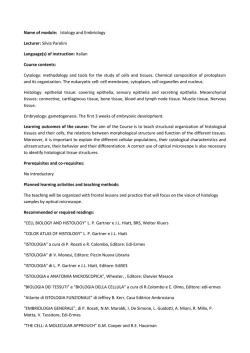
the same. A section of a portion of the retina reveals that is composed of
several layers (see Fig.1.1) in which ganglion cells (the output neurons of the
retina) lie innermost closest to the lens and front of the eye while photoreceptors (rods and cones) lie outermost against the pigment epithelium and
choroid. Light passes through several transparent nerve layers to reach the
rods and cones. A chemical change in the rods and cones send an electrical
signal back to the nerves. The signal goes rst to the bipolar and horizontal
6
cells, then to the amacrine cells and ganglion cells, then to the optic nerve
bres.
Figure 1.1: Section of the retina through its thickness. The image highlights
the neural structures.
The optic disc, a part of the retina sometimes called "the blind spot"
because it lacks photoreceptors, is located in the optic papilla, a nasal zone
where the optic-nerve bres leave the eye. The optic disc appears as an
oval white area of about 2x1.5mm. Temporal to this disc is the macula (see
Fig. 1.2). At its center, approximately 15mm to the left of the disc, is the
fovea, a spot measuring less than a quarter of a millimeter (200 µm) that is
responsible for sharp central vision. The circular eld of 6mm around the
fovea is considered the central retina, while the area beyond this is called
the peripheral retina.
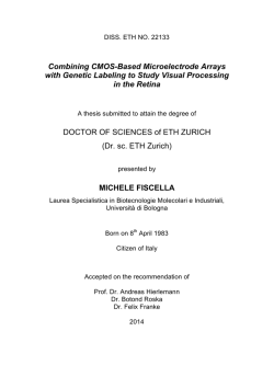
The retinal thickness shows great variations (see Fig. 1.3). The retina is
thinnest at the foveal oor (0.10, 0.150-0.200 mm) and thickest (0.23, 0.320
mm) at the foveal rim. Beyond the fovea the retina rapidly thins until the
equator. At the ora serrata the retina is thinnest (0.080 mm).
7
Figure 1.2: Sectional detail of the retina along the superior-inferior axis of
a left human eye through the optic nerve, showing details of the vascular
supply in this location.
Figure 1.3: The variation of human retinal thickness in mm around the fovea
(data from Sigelman and Ozanics (1982)).
1.1.1
Retinal vascular network.
There are two sources of blood supply to the mammalian retina: the central
retina artery (CRA) and the choroidal blood vessels. The choroid vessels
provide the greatest blood ow (65-85%) and are vital for the maintenance
of the outer retina (particularly the photoreceptores). The remaining 20-30%
blood ow to the retina comes from the central retina artery (see Fig. 1.4).
Within the optic nerve, the CRA divides to form two major trunks and each
of these divides again to form the superior nasal and temporal and the inferior
nasal and temporal arteries that supply the four quadrants of the retina.The
retinal venous branches are distributed in a similar fashion. The vessels
emerge from the optic nerve and run in a radial fashion curving toward and
around the fovea. The major arterial and venous branches and the successive
8
divisions of the retinal vasculature are present in the nerve ber layer close to
the internal limiting membrane. The retinal arterial circulation in the human
eye is a terminal system with no arteriovenous anastomoses (communication
between vessels) or communication with other arterial systems: thus, the
blood supply to a specic retinal quadrant comes exclusively from the specic
retinal arteries and veins that supply that quadrant, and any blockage of
blood supply results into infarction.
Figure 1.4: Section of the retina with the distribution of blood vessels.
taken from [2]
Figure
As the large arteries extend in the retina towards the periphery they
divide to form arteries with progressively smaller diameter, until they reach
the point where they return continuously to the venous drainage system.
This process of division occurs either dichotomously or at right angles to
the original vessels. The terminal arterioles and venules form an extensive
capillary network in the inner retina as far as the external border of the inner
nuclear layer.
The retinal vasculature is structured in three distinct layers: the supercial
(innermost) layer, the intermediate layer, within ganglion cells layer, and
the deep layer, within the inner nuclear layer (see Fig. 1.4). The larger
vessels lay in the innermost layer, whereas a plexus of capillaries occupy
the other two layers with precapillary arterioles and postcapillary venules
linking them to larger vessels. Blood ow of the arterioles in the supercial
9
layer is directed to the intermediate and deep layers of the retina. Normally,
no blood vessels from the the CRA extend into the outer plexiform layer,
the layer that divides the photoreceptores layer to the other layers. Thus,
the photoreceptor layer of the retina is free of the blood vessels supplied by
the CRA. The choriocapillaries provide the blood supply to photoreceptors.
Since the fovea contains only photoreceptores, this cone-rich area is free
of any branches from the CRA. The walls of all blood vessels except the
capillaries are composed of three distinct layers, or tunics (see Fig. 1.5).
The tunics surround a central blood-containing space called the lumen. The
inner most tunic, which is in intimate contact with the blood, is the tunica
intima. It contains the endothelium that lines the lumen of the vessel, and its
at cells t closely together, forming a slick surface that minimizes friction.
The endothelial cells of the retinal arteries are linked by tight junctions that
establish a blood-retinal barrier to prevent the movement of large molecules
or plasma proteins in or out of the retinal vessels. The middle layer, the
tunica media consists mostly of one or more layer of smooth muscle cells
(SMCs). Since small changes in blood vessel diameter greatly inuence blood
ow and blood pressure, the activities of the tunica media are critical in
regulating circulatory dynamics. The tunica media is usually the bulkiest
layer in arteries.
Figure 1.5: Schematic structure of the wall of blood vessels.
The outer most layer is the tunica adventitia and is composed of loosely
woven collagen brils that protect the vessel and anchor it to surrounding
structures. Capillaries are the smallest blood vessels. Their exceedingly thin
walls consist of just a thin tunica intima. Unlike the arteries and veins, capillaries are very thin and fragile. They are so thin that blood cells can only pass
10
through them in single le. The capillary wall is composed of three distinct
elements: endothelial cells, intramural pericytes and a basement lamina. The
exchange of oxygen and carbon dioxide takes place through the thin capillary wall. The red blood cells inside the capillary release their oxygen which
passes through the wall and into the surrounding tissue. The tissue releases
its waste products, like carbon dioxide, which passes through the wall and
into the red blood cells. The continuous endothelial cell layer is surrounded
by a basal lamina within which pericytes form a discontinuous layer in almost a one to one ratio with endothelial cells. Like SMCs, pericytes provide
structural support to the vasculature and represent the myogenic mechanism
for vasculature autoregulation of blood ow in response to changes in neural
activity. They are able to regulate the capillary diameter through contraction and relaxation. Pericytes are also involved in the regulation of vascular
permeability.
Arteries and veins physiology. In the human retina arteries and veins
accompany each other, but they are distinguished based on the branching
pattern and the size of the vessels. Pattern. The arteries tend to have
'Y-shape' branches with arms of equal diameter at the equator and at the
periphery of the retina. They give rise to side-arm branches which then progressively divide into dichotomic branches of arterioles. The arterioles give
rise to capillaries. As in the arteries, side-arm branches also arise from the
veins, and give rise to venule branches. Unlike the arterioles, the venules are
more likely to have a 'conveying type' branching pattern, which is also known
as strictly asymmetric branching. There are veins which are sensitively bigger than other, and they have a 'T-shape' and give uneven size to the whole
veins network. The arterioles with the delivery branching pattern are more
spaced out in comparison with the vessels with the conveting branching pattern. Measurements. The arteries around the optic nerve are approximately
100µm in diameter, with 18µm thick walls - then they decrease in diameter,
until the branched arteries lying in the deeper retina reach 15µm. The major
branches of the central veins close to the optic disk have a lumen of nearly
200µm with a thin wall made up of a single layer of endothelial cells having
a thin basement membrane (0.1µm). The lack of smooth muscle cells in the
venular vessel wall results in a loss of a rigid structural framework for such
vessels, resulting in shape changes under condition of sluggish blood ow
(e.g, diabetes) or with increased venous pressure. The retinal arteries have
a thicker muscular layer, which allows increased constriction in response to
pressure and chemical stimuli.
Blood ow of the supercial layer containing large vessels is mostly directed
to the vasculature at the intermediate and deep layers of the retina, as it is
shown in Figure 1.6.
11
Capillary physiology. Pattern. The retinal capillary network is spread
throughout the retina, diusely distributed between the arterial and venous
systems in the intermediate layer and in the deep layer, and it is anostomotic. The capillaries are connected in tri-junction connection pattern, in
which each capillary is connected to two other capillaries. The capillaries
either form a 'loop' shape if they are distributed in the same layer, or move
transversely to connect vessels in the other layers. In the human retina a
regional variation of the density of capillary distribution is reported: the capillary distribution at the equator region is denser than that in the peripheral
region. Measurements. There are three specic areas of the retina that are
devoid of capillaries, the 400 µm wide area centred around the fovea, the
one adjacent to the major vessels and the retinal periphery. The capillaries
network extends as far peripherally as retinal arteries and veins. The retinal
capillary lumen is extremely small (3.5-6 µm in diameter). Like capillary
networks elsewhere in the body, the retinal capillaries assume a meshwork
conguration to ensure adequate perfusion to all retinal cells. The deep capillary layer has mesh diameter (i.e., the distance between capillaries) that
averages 50µm in diameter but varies between 15 and 130 µm. The more
supercial capillary layer has slightly larger meshwork, on average 65µm in
diameter (16 to 150µm). In the mid-equatorial and anterior zones, where
the retina is thinner, only one capillary layer is present.
Figure 1.6: Schematic representation of the retinal layers and the connection
between vessels.
12
1.2
Geometrical Models of the Retina
Although it would be necessary to study uid ow and transport of solutes in
a real structure of the retina from medical imaging, this is beyond the scopes
of the present work. Moreover, we would need a large number of parameters,
which in some cases are dicult to determine experimentally (for example
the distribution of the large number of capillaries in the capillary beds).
Therefore, we use articial mathematical structures to describe the retina.
The results we get are in good agrement with experimental data showing
that we use an acceptable modelization of the real geometry. In this chapter
we discuss the geometrical models used to describe the arteriolar tree, the
capillary bed and the tissue, respectively.
1.2.1
Arteriolar Tree
We present two types of vascular tree structures that we use in our studies.
First, we describe the structure proposed in [20], a dichotomic branching
system, then we describe a structure more similar to the real retina based
on fractals.
1.2.1.1 Dichotomic Tree
In their paper [20], Takahashi and Nagaoka develop a theoretical and mathematical concept to quantitatively describe the hemodynamic behaviour in
the microvascular network of the human retina. A dichotomic symmetric
branching network of the retinal vasculature is constructed, based on a combination of Murray's law and a mathematical model of fractal vascular trees.
The optimal branching structure of a vascular tree is given by Q = krm ,
where Q is the volumetric ow rate, r is the inner radius of the vessel segment, k is a constant, and m a junction exponent which ranges between
2.7 and 3, as shown [19][17]. In [20], the constant m is set equal to 2.85,
a value that is more suitable for application to the retinal microcirculation
(see Fig. 1.7). It is proved mathematically that the exponent m is the sum of
a fractal dimension (D) and a branch exponent (α). Takahashi et al. apply
a fractal dimension of 1.70 and a branch exponent of 1.15.
The fractal dimension can quantify the property of a complex vascular network, and the value of α can also quantitatively dene the relation between
the length and radius of a branch segment as
L(r) = 7.4rα .
(1.1)
The equation is derived from data on cerebral vessels, but it is known from
studies that the vasculature of the retina and brain are similar.
13
Figure 1.7: Ratio of larger daughter-branch diameters to their mother-branch
diameters vs asymmetry ratio of the larger to the smaller daughter branch
diameters at some bifurcations in the human retina. Dotted and solid line:
curves predicted by Murray's Law with diameter exponent 3 and 2.85 respectively. Scattered data from photographed normal human eye.(Figure taken
from [20])
Combining Q = kr2.85 with conservation of mass ow rate, the conguration of a dichotomic vascular tree at every branching point can be expressed
by
2.85
2.85
+ r2,2
(1.2)
r12.85 = r2,1
where r1 is the radius of a mother branch, and r2,1 and r2,2 are the radii of
daughter branches at the same bifurcation. The larger arteriole, that originates directly from the central retinal artery (CRA), is given a generation
number of 1. Branches of respectively arteriole 1 are given a generation number of 2, and subsequent generations are formed in an identical fashion until
the ospring decreases about 6 µm in diameter. Individual precapillary vessels instead spread out into four true capillaries vessels, and then join again
to form a single postcapillary venule, as shown in Fig. 1.8.
14
Figure 1.8: Microvascular arterial network topologically represented as a successively repeating dichotomic branching system. Each parent vessel gives
rise to two osprings, each of the osprings gives rise to further two osprings, and so on. Four capillaries are assumed to divide from each precapillary. (Figure taken from [20])
In our study, we consider a network with 10 generations. The diameters
decrease from the larger arteriole, which has a diameter of 108 µm, value
taken as an input data for the model, through small arterioles to precapillaries, with diameter of 12.1µm.
Figure 1.9: Distribution of diameters as a function of the hierarchical level.
15
1.2.1.2 Diusion-limited aggregation model (DLA)
The application of fractals and fractal growth processes to the branching
blood vessels of the normal human retinal circulation was introduced by
Masters and Patt in 1989 [12]. Growing, branching objects can be reproduced by computer simulations in which the spatial dependence of a eld
satises the Laplace equation with moving boundary conditions. A class of
processes based on fractal growth is the diusion-limited aggregation model
(DLA) proposed by Witten and Sander in 1981 [23], and applicable to aggregation in any system where diusion is the primary means of transport
in the system. DLA can be described as the process whereby a single particle performs a random walk until it accidently hits an existing immobile
aggregate. Then, the particle attaches to the cluster and becomes immobile.
Besides this irreversible sticking no interaction of particles is present. This
extremely simple process produces surprisingly complex, branched objects
which are very appealing from a scientic point of view and have evidence
in natural phenomena. This is, for instance, approximately the case when
water molecules form a snow ake. Under appropriate conditions, the vicinity of the ake contains almost no water and molecules have to cross this
water poor region by means of Brownian motion before they can attach to
the growing aggregate. Another example is the electrolytic deposition of
material on an electrode. If the present electric eld is not too large, the
motion of ions will be dominated by diusion.
The simulation of a DLA yields branching patterns similar to the branching
patterns seen in the human retina. Moreover, a series of papers led to an
estimate of the fractal dimension for the retinal vessels of D = 1.7, which
is in good agreement with the dimension of a diusion-limited aggregation
cluster grown in two dimensions that is usually D = 1.71 . The fractal dimension is dened as D = ln(M )/ln(R) where R is the radius of the cluster,
the maximum distance between the rst particle to another, and M its mass
(i.e. the number of the particles that form the cluster).
In our study, we have used a Matlab code to obtain DLA clusters, an
example of which is depicted in Fig. 1.10. To build it, we consider a mass
M = 3000 and a maximum radius R = 300. Then we use the Hit-and-Miss
lter, a binary morphological operators, with few structuring elements to
modify the cluster (see Fig. 1.11), so that:
• segments of the cluster are formed by a single pixel in width (a procedure similar to skeletonization);
• segments do not intersect forming closed regions (loops);
• each line has at most two forks.
16
We note that though the mass of B in Fig. 1.10 is lower than the original
DLA, the fractal dimension is still similar to the value of retinal fractal
dimension.
Since the retina has an area of about 1089 mm2 (72% of a sphere about
22mm in diameter), we set a pixel to be equivalent to approximately κ µm
(κ depends on the size of the matrix representing the gure, in our case
κ = 162µm). In this way, we can determine the length of the various segments
in the DLA system.
Figure 1.10: A) The original DLA cluster. B) The
application of the morphological operator.
DLA cluster after the
Figure 1.11: A) A particular of the original cluster. B), C) and D) are the
same object as in A) after some application of the morphological operator.
In B) each segment has a width of one pixel, C) shows a deleted loop, while
D) shows a deleted trifurcation.
17
Then we determine the four major arteries, and we assign to these a
radius that decreases as one moves away from the center, between 54 and
15 µm. We assign to smaller branches a value which decreases moving away
from the main branches from 15 to 5 µm.
Figure 1.12: Colours represent the values of the radii of the vessel branches.
Larger radii correspond to the four major arteries.
18
1.2.2
Capillary Plexi
The capillaries are the main location where the transport of nutrients between blood and tissue takes place.
The number of capillaries is huge and the structure of the capillary plexus
is very complex. The retinal capillaries are embedded in the retinal tissue
and each of these has to be described by mathematical laws very dierent
from each other. Therefore we must treat the tissue and the capillaries as
two separated domains.
In the retinal tissue its individual components are not densely packed. Therefore the interstitial uid can ow freely within the tissue. For this reason,
the retinal tissue can be described as a porous medium with a single phase
ow, where with phase we mean a matter that has a homogeneous chemical
composition and physical state (in this case uid). The composition of interstitial uid is similar to blood plasma, which consists by 90% of water.
In the capillary bed, to avoid the high computational expenses that we incur if we use a discrete approach, can be introduced a capillary continuum,
which represents the capillary bed around the tissue as averaged quantity.
Hence, capillary bed can be described as a porous medium with a uid phase,
the blood, where the medium is represented by the tissue. To pass from a
discrete to a continuum description, we use the concept of a representative
elementary volume (REV) and we dene new eective parameters, as porosity, tortuosity or permeability.
For these reasons, we use a double continuum approach [5], in which the heterogeneous domain of capillary plexus is represented by two separate, but
spatially overlapping and interacting continua, one consisting of the capillaries and the tissue and the other of the interstitial uid and the tissue
(see Fig.1.13). At any point of the capillary plexus domain two values for
each eective parameter are dened: one for the capillaries and one for the
interstitial uid within tissue.
19
Figure 1.13: Schematic illustration of the general concept of the doublecontinuum model.(Figure taken from [5])
20
1.2.3
Tissue with layers
Anatomically, the retina is usually considered to consist of two main parts,
the outer retina (which is avascular) and the inner retina (which is supplied with blood). Moreover, it has a distinctly layered structure in which
oxygen sources and consumption are more compartmentalised than in other
tissues. The oxygen required in the retina is primarily derived from blood
in choroidal vessels and in the central retina artery. The choroidal blood
vessels supply oxygen to the outer retina whereas the central retina artery
supplies the inner retina.
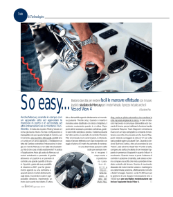
In this study, we assume that the retinal tissue is divided in eight layers
(see Fig. 1.14), based on their anatomical and functional properties [3]-[4].
The outer retina is formed by three layers: outer segments of the photoreceptors layer, inner segments of the photoreceptors layer and outer nuclear
layer. The inner retina is divided in ve layers: outer plexiform layer, inner nuclear layer, outer region of the inner plexiform layer, inner region of
the inner plexiform layer and Ganglion cell/nerve bre layer. Most of the
oxygen delivered by choroidal circulation to the outer retina is consumed by
inner segments of the photoreceptors because in this layer are localized the
majority of photoreceptors. A greater portion of the oxygen provided by
the retinal circulation to the inner retina is utilized by the inner plexiform
layer. Therefore, we will assume that the consumption of oxygen takes place
only in these two layers. In the Ganglion cell/nerve bre layer is located
the supercial capillary bed while in the outer plexiform layer is it the deep
capillary bed.
21
Figure 1.14: Scheme of retinal layers. Layer 1=outer segments of thephotoreceptors layer, Layer 2=inner segments of the photoreceptors layer,Layer
3 = and outer nuclear layer, Layer 4 = outer plexiform layer, Layer 5 = inner
nuclear layer, Layer 6 = outer region of the inner plexiform layer,Layer 7 =
inner region of the inner plexiform layer, Layer 8 = Ganglion cell/nerve bre
layer.(Figure taken from [3])
22
Chapter 2
Models of Blood Flow
The circulatory system in general, and so also the human retina we are
analyzing, consists of a network of many interconnected vessels, and the ow
through any segment depends not only on the ow resistance of that segment
but also on the resistance of other vessels connected to it in series and in
parallel.
Theoretical modeling, in combination with experimental studies, has the
potential to synthesize several observed or hypothesized mechanisms into a
unied mathematical framework. The model can then be used to predict the
overall behavior of the system, taking into account the interactions between
dierent mechanisms occurring at the level of individual cells or segments
and the interactions that arise in a network of interconnected segments. In
this chapter we rst introduce the Hagen-Poiseuille model for ow through
ducts, which provides a reasonable estimation for blood ow through vessels.
Then we present two models for the distribution of hemodynamic parameters
in the human retina.
2.1
Flow in the arteriolar tree
Flow in the arteriolar tree is supposed to be of Hagen-Poiseuille type.
Poiseuille ows are generated by pressure gradients, with application primarily to ducts. They are named after J.L.M. Poiseuille (1840), a French
physician who experimented with low-speed ow in tubes.
Consider a straight duct of arbitrary but constant shape. There will be an
entrance eect, i.e. a thin initial shear layer and core acceleration (see Figure 2.1). The shear layers grow and meet, and the core disappears within a
fairly short entrance length,Le .
For x > Le the velocity becomes purely axial and varies only with the lateral coordinates, so v = w = 0 and u = u(y, z) (see Figure 2.2). The ow is
then said to be fully developed. For fully developed ow the continuity and
23
Figure 2.1: Flow in the entry region of a tube.
(Figure taken from [22])
momentum equations for incompressible ows reduce to:


 ∂u = 0



∂x




2

∂p
∂ u ∂2u
0=−
+µ
+

∂x
∂y 2
∂z 2






∂p
∂p


=−
0=−
∂y
∂z
These equations indicate that the total pressure p is a function only of x for
this fully developed ow. Further, since u does not vary with x, it follows
from the x-momentum equation that the gradient ∂p/∂x must only be a
negative constant. The basic equation of fully developed duct ow is thus:
2
∂ u ∂2u
1 ∂p
+ 2 =
= const
(2.2)
∂y 2
∂z
µ ∂x
Note that the acceleration terms vanish here, since the ow is very slow.
24
Figure 2.2: Fully developed duct ow.
(Figure taken from [22])
Flow through a circular pipe
The ow through a circular pipe with radius R was rst studied by Hagen
(1839) and Poiseuille (1840). The Laplace operator in polar coordinates
under the hypothesis of radial symmetry and axial invariance reduces to:
1 d
d
2
∇ =
r
r dr
dr
and, under these hypothesis, the solution of the fully developed equation
ow, Eq. (2.2) is
1 ∂p 2
u(r) =
( )r + C1 lnr + C2 .
4µ ∂x
Since the velocity cannot be innite at the centerline we reject the logarithm
term and set C1 = 0. The no-slip condition is satised by setting C2 = 41 .
The pipe-ow solution is thus:
u=−
dp/dx 2
(R − r2 ),
4µ
so that the velocity distribution in fully developed laminar pipe ow is a
paraboloid of revolution about the centerline (Poiseuille paraboloid, see Figure 2.3).
The total volume rate of ow Q is
Z
Q=
udA,
section
which for the circular pipe gives
Qpipe =
πR4
8µ
25
dp
−
.
dx
(2.3)
Figure 2.3: Parabolic ow in a circular pipe.
The mean velocity is dened by v = Q/A and gives, in this case
Qpipe
.
πR2
Finally, the wall shear stress is constant and given by
1
du
dp
4µv
= R −
τw = µ −
=
.
dr w
2
dx
R
v=
2.1.1
(2.4)
Model equations
It is assumed that blood ow conforms to Hagen-Poiseuille's law in each vessel channel through consecutive bifurcations of the retinal microvasculature,
and that the movement of material across the exchange vessels is balanced
between blood and tissue.
Hagen-Poiseuille's law indicates that the decrease in pressure ∆P against
ow Q(r) along a branch of radius r and length L(r) can be written as:
∆P =
8µ(r)L(r)Q(r)
,
πr4
(2.5)
where µ(r) is the apparent viscosity of blood that depends on the size of
the vessel, and is supposed to follow a mathematical expression proposed by
Haynes in [9],
µ∞
µ(r) =
,
(2.6)
(1 + δ/r)2
where µ∞ is the asymptotic blood viscosity, set to 3.2·102 Poise and δ = 4.29.
Blood ow exerts a tangential force that acts on the luminal surface of the
blood vessel as τw (r) wall shear stress
τw (r) = µ(r)γw (r),
(2.7)
4Q
4v
=
3
πr
r
(2.8)
γw (r) =
26
where γw (r) is the shear rate at the wall surface.
For the conservation of ow, as represented in Figure 2.5, for each bifurcation
node the inow must be the same as the outow:
Qin = Qout
(2.9)
where Qin is the total inow and Qout is the total outow.
We observe that the vascular tree has analogies with a classical electrical
circuit: we can interpret the blood ow Q through vessels as the intensity of
current I , the pressure drop ∆P as the potential dierence ∆V , and nally
the conductance of the vessel as the conductance of the circuit, that is the
inverse of the resistance R.
Figure 2.4: Electrical circuit which represents an dichotomous arterial vasculature.
Figure 2.5: Conservation of ow (i.e. intensity of current) in a generic network tree: in each nodePi the outow in the adjacent nodes must equal the
inow so that we have j∈Adj(i) Iij = Ii
27
Remembering the Hagen-Poiseuille pressure drop equation:
8µL
Q,
πr4
∆P =
and comparing it with the equation governing the current ow through electrical network
∆V = Ri
we can see that the expression 8µL
is an equivalent of the resistance R for
πr4
blood ow. We dene its inverse:
G=
πr4
8µL
(2.10)
as the conductance of the network. To be precise, in each bifurcation node i,
where a vessel ends splitting into two daughter branches ij directed to nodes
j , the vessel conductance (vessel connecting node i and node j ) is dened as
follows:
4
πrij
Gij =
(2.11)
8µij Lij
where rij is the radius of the vessel at generation i, Lij the vessel length (the
lengths of the two branches are equal for symmetry), and µij the viscosity
of the vessel.
Extending these node properties to the whole tree level and combining it
with the conservation of ow we get an equivalent of Kirchho law for blood
ow:
X
X
Qij =
Gij (Pi − Pj ) = 0,
(2.12)
j∈Adj(i)
j∈Adj(i)
where Adj(i) is the set of indexes of network nodes adjacent to node i, Pi
and Pj are the pressures at the nodes i and j respectively. Subsequently, we
can compute the blood ow in the single vessels Qij using:
!−1
4
πrij
Qij
Pi − Pj = ∆Pij =
8muij Lij
=⇒ Qij = ∆Pij Gij .
(2.13)
Boundary nodal pressures are required to start the computation. The
boundary inlet node is the artery of generation 1, where the blood ow
enters the network. The boundary outlet nodes are the nodes where the
blood ow exits the network, in our case the capillaries.
In the case of binary network at each bifurcation nodes, because of the
symmetry of the network, the blood ow divides itself equally into the two
daughter branches:
28
Q1 (r1 ) = 2Q2 (r2 ) = ... = 2g−1 Qg (rg ),
and
−(g−1)
vg = 2
r1
rg
2
v1,
where r1 and v 1 are the radius and mean ow velocity of the trunk vessel of
generation 1 and g is the generic g − th ospring.
29
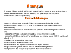
2.1.2
Numerical results
Using the model equations illustrated in the previous sections, we have computed the values of hemodynamic parameters using the binary tree and DLA
network, respectively. The blood pressure at the rst artery was estimated
by considering the hydrostatic and frictional pressure losses from the aorta
to the central retina artery, and xed at a value of 40mmHg. We consider
two conditions for the blood pressure at the outlet of the system:
• in a rst condition, we assume that 60% of nal branches goes into deep
capillary layer and that 30% goes into supercial capillary layer. We
increase the length of these branches by a length equal to the distance
between the plane of the arterial system and the respective planes of
the capillaries. We set the partial pressure equal to 20mmHg in all
nal branches.
• in a second condition, we set, in each nal branch, a xed blood pressure at the outlet of the system equal to 20mmHg.
In the binary model, we use both cases for the pressure at the outlet of the
system. In the DLA model, we use only the rst condition in its center and
we set the branches in its periphery as branches ending at the level of the
arterial system. If we compare the arterial tree to an electric circuit, we
treat the coupling between the capillary bed and arterial tree by inserting
in the branches of the system that descend to this an equivalent resistance
in parallel, which is calculated by comparing the capillary bed to a circuit
formed by a 600 square mesh. The calculation of the equivalent resistance is
described in the appendix. In this study we consider an equivalent resistance
equal to 1e11g/cm4 s, which we have obtained by considering the capillaries
of radius 2.5µm and length 50µm. Moreover, the coupling between arterial
tree and surrounding tissue in the branches that end in the arterial layer
is treated inserting an equivalent resistance. We set this value equal to
5e8g/cm4 s.
The results are shown in the next gures. We compare the values of
mean velocity and mean ow rate that we get in the vascular system with
data measured in Riva et al [15].
30
Figure 2.6: Distribution of mean blood pressure in the binary tree model
as a function of vessel diameter. These values are obtained by imposing an
outlet pressure equal to 20 mmHg .
Figure 2.7: Distribution of mean blood pressure in the binary tree model as a
function of vessel diameter. These values are obtained by imposing an outlet
pressure equal to 20 mmHg and requiring that 60 % of nal branches goes
into deep capillary layer, 30 % goes into the supercial capillary bed the other
part terminates in the arterial layer. The uctuations of mean pressure in
correspondance with each value of the vessel diameter are caused by increased
resistance of some nal branches to make the coupling to capillary beds.
31
Figure 2.8: Distribution of mean blood pressure in the DLA system as a
function of vessel diameter. These values are obtained by imposing an outlet
pressure equal to 20 mmHg and requiring that peripherical nal branches
terminate in the arterial layer, while internal nal branches are such that
60 % of these goes into deep capillary bed, 30 % goes into the supercial
capillary bed. The high uctuations of mean pressure around the diameter
value of 30µm are caused by the existence of nal branches near the input
of DLA system.
Figure 2.9: Distribution of mean velocity in the binary tree model compared
with experimental data in Riva et al. [15] as a function of vessel diameter .
These values are obtained by imposing an outlet pressure equal to 20 mmHg
.
32
Figure 2.10: Distribution of mean velocity in the binary tree model compared
with experimental data in Riva et al. [15] as a function of vessel diameter .
These values are obtained by imposing an outlet pressure equal to 20 mmHg
and requiring that 60 % of nal branches goes into deep capillary layer, 30
% goes into the supercial capillary bed and the other part terminates in
the arterial layer. The uctuations of mean velocity in correspondance with
each value of the vessel diameter are caused by increased resistance of some
nal branches to make the coupling to capillaries beds. The highest values
of mean velocity correspond to branches that end in the arterial layer.
33
Figure 2.11: Distribution of mean velocity in the DLA model compared
with experimental data in Riva et al. [15] as a function of vessel diameter.
These values are obtained by imposing an outlet pressure equal to 20 mmHg
and requiring that peripherical nal branches terminate in the arterial layer,
while internal nal branches are such that 60 % of these goes into deep
capillary bed, 30 % goes into the supercial capillary bed. The highest
values of mean velocity are located in the central branches that end in the
arterial layer. The results that are obtained with the DLA model are in
closer agreement with the experimental data than those obtained with the
binary tree model.
34
Figure 2.12: Distribution of mean ow rate in the binary tree model compared with experimental data in Riva et al. [15] as a function of vessel
diameter. These values are obtained by imposing an outlet pressure equal
to 20 mmHg .
Figure 2.13: Distribution of mean ow rate in the binary tree model compared with experimental data in Riva et al. [15] as a function of vessel
diameter. These values are obtained by imposing an outlet pressure equal to
20 mmHg and requiring that 60 % of nal branches goes into deep capillary
layer, 30 % goes into the supercial capillary bed the other part terminates
in the arterial layer. The uctuations of mean ow rate in correspondance
with each value of the vessel diameter are caused by increased resistance of
some nal branches to make the coupling to capillaries beds.
35
Figure 2.14: Distribution of mean ow rate in the DLA model compared
with experimental data in Riva et al. [15] as a function of vessel diameter.
These values are obtained by imposing an outlet pressure equal to 20 mmHg
and requiring that peripherical nal branches terminate in the arterial layer,
while internal nal branches are such that 60 % of these goes into deep
capillary bed, 30 % goes into the supercial capillary bed. The highest
values of mean ow rate are located in the central branches that end in the
arterial layer. The results that are obtained with the DLA model are in
closer accordance with the experimental data than those obtained with the
binary tree model.
36
The wall shear stress at the precapillary vessels increases, since the apparent viscosity increases due to the geometrical obstacle encountered by
the red blood cells owing in these narrow channels. The wall shear stress
of the vessels at the pre-equator and equator region is signicantly higher
than that at the periphery region, see [6]. This is reasonable because the
uid is owing outward from the center of the retina, hence the further from
the center the lower the pressure is. As a result, the driving force for the
ow in the arteriolar branches at the pre-equator region is higher than at
the periphery, hence the wall shear stress is higher.
This leads to an observation on the relationship between the high wall shear
stress and the vessel wall thickness of arterial vessels near the pre-equator
and equator regions.
The wall of retinal arteries near the optic disc (pre-equator region) comprises
ve to seven layers of smooth muscles. At the equator and periphery, however, the arterial wall has only two or three and one or two muscle layers,
respectively. This seems to suggest that the vessels at the pre-equator and
equator regions have adapted themselves by increasing their wall thickness
(i.e., smooth muscles) to sustain the higher wall shear stress.
Figure 2.15: Distribution of mean shear stress in the binary tree system as
a function of vessel diameter. These values are obtained by imposing outlet
pressure equal to 20 mmHg .
37
Figure 2.16: Distribution of mean shear stress in the binary tree system as
a function of vessel diameter. These values are obtained by imposing outlet
pressure equal to 20 mmHg and requiring that 60 % of nal branches goes
into deep capillary layer, 30 % goes into the supercial capillary bed the
other part terminates in the arterial layer. The uctuations of mean shear
stress in correspondance with each value of the vessel diameter are caused by
increased resistance of some nal branches to make the coupling to capillary
beds.
38
Figure 2.17: Distribution of mean shear stress in DLA system as a function
of vessel diameter. These values are obtained by imposing an outlet pressure
equal to 20 mmHg and requiring that peripherical nal branches terminate
in the arterial layer, while internal nal branches are such that 60 % of these
goes into deep capillary bed, 30 % goes into the supercial capillary bed.
The highest values of mean shear stress are located in the central branches
that end in the arterial layer.
39
Figure 2.18: The plot represents the spatial distribution of mean blood pressure in the DLA system. The colors represent the values of this. The pressure decreases along the main artery from the center to the periphery, to
reach 20mmHg. The lowest pressures at the center of system are caused by
imposing the Dirichlet boundary conditions.
40
Figure 2.19: The plot represents the spatial distribution of mean velocity in
the DLA system. The colors represent the values of this. The mean velocity
decreases along the main artery reaching very low levels in the periphery.
The highest values of the velocity correspond to the vessels that end in
the arterial plane and this fact is due to the high resistance applied to the
branches that descend into the capillary beds.
41
Figure 2.20: The plot represents the spatial distribution of mean ow rate
in the DLA system. The colors represent the values of this. The mean ow
rate decreases along the main artery reaching low values in the periphery.
42
Figure 2.21: The plot represents the spatial distribution of mean shear stress
in the DLA system. The colors represent the values of this. The highest vales
of mean shear stress correspond to the vessels in which there are the highest
values of mean velocity. Also, between these vessels, the value of mean shear
stress is greatest if the radius is smallest.
43
2.2
Flow in Capillary Plexi and in Interstitial Tissue
The retinal capillaries are embedded in the retinal tissue, but these domains
are very dierent from each other. To describe these, we use the doublecontinuum approach that we presented in Ch.1 in which they are treated
as two separate continua coupled by exchange functions. In this section we
briey describe the equations that govern the uid ow in these domains.
Retinal Tissue
Since we consider interstitial tissue as a porous medium, the ow velocity of
the interstitial uid can be described by Darcy's law:
K
→
−
v F = − (∇P ),
µ
(2.14)
−
where →
v F is the Darcy velocity, K is the intrinsic permeability tensor and
µ the uid viscosity of the uid phase.
The conservation of mass is expressed by the following equation:
−
∇ · (ρT →
v F ) + q − qF = 0
(2.15)
where ρT is the apparent mass density, i.e. the intrinsic mass density of uid
per unit volume (ρtissue ) multiplied by the volume fraction of tissue within
the model domain (fT = Vtissue /Vtot ), q represents the external sources or
sink (e.g. the inuence of the lymphatic system, that can be seen as a sink),
qF is the coupling variable for the ow between the two continua. Since
we consider a incompressible uid phase and a constant tissue porosity φ,
the temporal variation of the product of φ and ρT is not considered in the
continuity equation.
Retinal Capillary
As in the case of the retinal tissue, the capillary bed can be treated as
a porous medium, so that Darcy's law may be applied to determine the
blood ow velocity. The ow of blood can be described with the following
continuity equation:
−
∇ · (ρC →
v F ) + qF = 0
(2.16)
where ρC is the apparent mass density, i.e. the intrinsic mass density of uid
per unit volume (ρblood ) multiplied by the volume fraction of tissue within the
model domain (fC = Vcapillary /Vtot ), qF is the coupling variable for the ow
between the two continua. Since we consider a incompressible uid phase
and a constant tissue porosity φ = 1, the temporal variation of the product
of φ and ρC is not considered in the continuity equation.
44
Coupling Tissue-Capillary
The exchange of uid across the capillary walls into the retinal tissue and
vice-versa, is governed by an exchange term, the transfer or coupling function qF , that depends on the uid pressure gradient across the vessel wall.
According to Starling's law, net uid ow across a vessel wall is given by:
qF = ρmol Lp
Avessel
(Pc − Pis )
Vtissue
(2.17)
where Lp is the hydraulic conductivity of the vessel wall, Avessel /Vtissue is the
surface area of the retinal capillaries per unit volume of tissue and ρmol is the
intrinsic mass density of uid that passes from capillary into the interstitium
across the microvascular wall. The term within parenthesis is called the
transmural pressure, where pc and pis are the uid pressure in capillaries
and interstitial space, respectively.
2.2.1
Calculation of Permeability in Capillary Bed
In this section, we present the computation of the continuum intrinsic permeability tensor in the capillary bed, that depends mainly on the connectivity
of the capillary segments and their size. We divide the capillary domain
into 600 rectangular cuboid subvolumes (see Fig.2.22 ) and we calculate the
permeability tensor as in Reichold et al.[14]. In the x-direction (in a similar
way in the y -direction) we have:
Kx =
Fx,REV µLx,REV
| PC − PA | Ay,z,REV
(2.18)
where Fx,REV is the mass ow between the two faces normal to the x-axis,
µ is the dynamic viscosity of blood, PA and PC are the pressures in A and C
respectively, Ay,z,REV is the cross section area of REV parallel to y -z -plane.
The volume of blood is:
Vblood ' 2πr2 Lx − (2r)3
(2.19)
and the porosity of blood is:
φblood =
Vblood
2πr2 Lx − (2r)3
=
.
VREV
L2x δ
(2.20)
To calculate the value of Kx , we set an arbitrary pressure boundary
condition PA and PC and no-ow boundary conditions on the face parallel
to x-z -plane and x-y -plane . Since we suppose a linear trend for the pressure
between A and C , the pressure value in B is (PC + PA )/2. because of
symmetry, we consider the cylinder between B and C and assuming HagenPoiseuille blood ow, Fx,REV is:
Fx,REV =
45
πr4 4P
4µLx
(2.21)
Figure 2.22: The REV. We consider Lx =50µm, δ =30µm and r=2.5µm.
where
4P =| PB − PC |=
| PC − PA |
.
2
Hence the permeability in the subvolume in x-direction is:
Kx =
πr4
.
8δLx
The numerical value of Kx is 0.01 µm2 .
46
(2.22)
Chapter 3
Models for Solute Transport
and Delivery
In this Chapter we present the models which describe the transport of a
solute from blood ow through the retina tissue. First, we describe solute
transport across the arterial wall using a Wall-Free model and a Multilayer
model, then we present a model for solute transport in the capillary bed
and in the retinal tissue. At the end of each section we adapt the model
equations in the case the solute is constituted by oxygen.
3.1
Solute transport across the vessel wall
A schematic radial cross-section of a vessel consists of: 1) a red blood cell-rich
core (RBC), 2) a red blood cell-depleted plasma layer (PL), 3) endothelial
vascular wall (ET), 4) smooth muscle layer (SMC) and 5) tissue space. The
lumen comprises the RBC and PL layers (see Fig. 3.1).
In our study we consider that the lumen of a vessel is not divided actually in
RBC and PL, but is a unique continuum. Each blood vessel is considered as a
cylinder of given radius Rv and length Lv in a three-dimensional system with
cylindrical coordinates. The z axis corresponds to the axis of the cylinder,
as in Fig. 3.2. The general geometrical structure of the model consists in
concentric cylinders as shown in Fig .3.2.
We denote by ΩL the lumen, ΩET the endothelial wall, ΩSM C the smooth
muscle layer and ΩT the tissue layer. We indicate by Γi the part of ∂Ωi
corresponding to the common interface between two distinct domains, by
→
−
n i the unit outward normal vector with respect to ∂Ωi and Ri the distance
of the interface Γi from the z axis. Moreover, in the following we will denote
by ΓL,in and ΓL,out the inlet and outlet section of the lumen, respectively.
47
Figure 3.1: Schematic cross-section of the model geometry showing the multilayer structure of the vessel: RBC-rich core (CR), RBC-depleted plasma
layer (PL), endothelial vessel wall (ET), smooth muscle cell (SMC), and
tissue space (TS).
Figure 3.2: The considered subdomains and the partitioning of the boundaries for the arterial wall model.
48
3.1.1
The Wall-Free Model
In this section we consider only a lumen as a physical domain ΩL , while the
presence of the arterial wall is expressed by a "transfer" boundary condition.
We suppose that the solute, in addition to being transported and diused
along the vessel, also lters throughout the wall of the vessel itself.
The equations that describe the transport and diusion of solute in ΩL
are:

∂P
∂2P
∂
1 ∂


r
+
+
(vz P ) = 0
−D

2

r
∂r
∂r
∂z
∂z







∂P →

 −D
·−
n L = γ(P − Pwall )
∂r





P = Pinlet








−
−
J ·→
n L,out − vn+ P = αP − Jout · →
n L,out
in ΩL ,
(3.1a)
on ΓL ,
(3.1b)
on ΓL,in ,
(3.1c)
on ΓL,out .
(3.1d)
where D is the diusion coecient of the solute that we suppose constant,
−
A the constant cross-section area of ΩL , →
v the velocity of the blood, P is
the solute partial pressure, Pwall is the solute partial pressure in the vascular
wall, γ is the solute permeability across the lumen-wall interface, J is a ux
of density mass and ∂Ω represent a wall of the vessel. We consider a Dirichlet
condition at the start of vessel (ΓL,in ) and a Robin condition at the end of
the vessel (ΓL,out ) [10]: Pinlet is the partial pressure at the inlet of domain,
Jout is the ux of density mass at the distal of domain and α is a constant
velocity .
We dene

−
−

vn = →
v ·→
n



v + = (v + |v |)/2
n
n
n
− = (v − |v |)/2

v
n
n

n


v = v + + v − .
n
n
n
It is convenient to dene a new variable Pav = Pav (z), the average of P
on the section area:
R 2π R R
Pav =
0
0
rP (r, z)drdθ
.
πR2
We integrate Eq.(3.1a) on the section, obtaining:
49
(3.2)
Z
0
2π
Z
0
R
∂
−D
∂r
Z R
Z R
∂2P
∂
∂P
−D 2 rdr +
r
dr +
(vz P ) rdr dθ = 0.
∂r
∂z
0
0 ∂z
Using the fundamental theorem of calculus in the rst term, we obtain:
Z R
Z R
∂2P
∂
∂P +
−D 2 rdr +
(vz P ) rdr = 0,
−DR
∂r ΓL
∂z
∂z
0
0
and using the boundary conditions, Eq.(3.1b),
Z R
Z R
∂2P
∂
Rγ(P − Pwall ) +
−D 2 rdr +
(vz P ) rdr = 0.
∂z
0
0 ∂z
(3.3)
Using Eq. 3.2 and assuming that the variation of v is small along z in the
blood vessel, we replace vz with vmean , and we approximate P on ΓL with
Pav . We obtain the following averaged model for the transport of solute in
the vessel:

2
∂J


+ 2 Rγ(Pav − Pwall ) = 0


∂z
R






∂P


 J = −D av + vmean Pav
∂z





Pav = Pinlet








−
−
J ·→
n L,out − vn+ Pav = αPav − Jout · →
n L,out
in ΩL ,
(3.4a)
in ΩL ,
(3.4b)
on ΓL,in ,
(3.4c)
on ΓL,out ,
(3.4d)
To describe the solute transport in each vessel of the arterial tree we use
Eq. (3.4a). Eqs (3.4c)-(3.4d) are used as boundary conditions at the inlet
and outlet of the arterial tree, respectively. At each bifurcation node s, we
assume the continuity of mass uxes through each section:
−
−
−
A J ·→
n =A J ·→
n +A J ·→
n ,
(3.5)
i i
i
j j
j
k k
k
where i,j and k are the names of vessels that have s as common node, A
−
represents the section area, J represents the density mass ux and →
n the
unit outward normal vector with respect to boundary of the vessel at the
bifurcation node.
We solve numerically the convection-diusion-reaction equations of the FreeWall Model using the FEM and the Scharfetter-Gummel method. These
methods are described in the appendix.
50
3.1.2
The Multilayer Model
In this section we study the same problem as in the previous section, but
whit a geometry that is more similar to the real one. We consider, in this
model, a lumen, an endothelium layer and a smooth muscle cell layer. The
presence of the tissue layer is expressed by a boundary condition (see Fig.3.2)
We suppose that the solute transport occurs within the arteriole space via
convection and diusion through the plasma. The general mass balance for
the solute inside the arteriole is given by:
−2π(rDL
∂I(Pav,L )
∂PL
)|ΓL +
= 0,
∂r
∂z
where
2
I(Pav,L ) = πRL
(−DL
∂Pav,L
+ vmean Pav,L ),
∂z
R 2π R RL
Pav,L =
0
in ΩL
0
PL (r, z)rdrdθ
,
2
πRL
and where vmean is the mean of blood velocity in the lumen, as in the previous section.
In this model, the transport of solute in the arterial wall is controlled by diffusion through this region and consumption by endothelial cells and smooth
muscle cells. The rate of solute consumption follows the Michaelis-Menten
kinetics. So the transport in the wall is described by the following equation:
Km,i Pi
1 ∂
∂Pi
−
rDi
+
=0
in Ωi
(3.6)
r ∂r
∂r
K1/2,i + Pi
where Pi = Pi (r) is the radial partial pressure of solute in the arteriole wall,
Di the diusion coecient, Km,i and K1/2,i the constants of the MichaelisMenten law. The subscript i indicates whether we are in endothelium layer
(ET) or smooth muscle cells layer (SMC). We assume continuity of the solute
partial pressure and the mass ux at each boundary interface, so that the
equations that describe the transport and diusion of solute in lumen and
wall are:
51

∂I(Pav,L )
∂PL


)|ΓL +
=0
−2π(rDL


∂r
∂z







Km,ET PET
∂PE
1 ∂


rDE
+
=0
−


r ∂r
∂r
K1/2,ET + PET







Km,SM C PSM C
1 ∂
∂PSM C


−
rDSM C
+
=0


r ∂r
∂r
K1/2,SM C + PSM C








Pav,L = Pinlet









−
−

J ·→
n L,out − vn+ Pav,L = αPav,L − Jout · →
n L,out




∂PET
∂PL



 −DL ∂r + DET ∂r = 0








PET = Pav,L (z = Lv /2)









∂PSM C
∂PET


+ DSM C
=0
−DET


∂r
∂r








PET = PSM C









∂PSM C



 DSM C ∂r + hW PSM C = hW PT
in ΩL ,
(3.7a)
in ΩET ,
(3.7b)
in ΩSM C , (3.7c)
on ΓL,in , (3.7d)
on ΓL,out , (3.7e)
on ΓL ,
(3.7f)
on ΓL ,
(3.7g)
on ΓET ,
(3.7h)
on ΓE ,
(3.7i)
on ΓSM C . (3.7j)
We use the FEM and Scharfetter-Gummel method with the assumption
of continuity of mass ux through each vessel section to solve the system
equations in (3.7) corresponding to the lumen. The FEM and ScharfetterGummel method are described in the Appendix.
The equations that describe the solute transport in the endothelium and
smooth muscle cells layers, Eqs. (3.7b)-(3.7c), are non-linear, for this reason
we use a xed point method to linearize and solve them. We approximate
the variable Pi with its mean across the radius of the layer, i.e.:
PET ' Pav,ET
1
:=
RET − RL
PSM C ' Pav,SM C
Z
RET
PET (r)dr
in ΩET ,
RL
1
:=
RSM C − RET
52
Z
RSM C
PSM C (r)dr
RET
in ΩSM C ,
and we obtain:
1 ∂
∂PET
−
rDET
+ γ(Pav,ET )PET = 0, in ΩET ,
r ∂r
∂r
∂PSM C
1 ∂
rDSM C
+ γ(Pav,SM C )PSM C = 0, in ΩSM C .
−
r ∂r
∂r
where
γ(Pav,i ) =
Km,i
K1/2,i + Pav,i
(3.8)
(3.9)
with i = ET, SM C
Eqs (3.8) and (3.9) have the form of the so-called modied Bessel equations
of order 0 (Kelvin's equations of order 0). Their solutions are [1]:
s
s
!
!
DET
DET
PET = AI0 r/
+ BK0 r/
in ΩET ,
γ(Pav,ET )
γ(Pav,ET )
s
s
!
!
DSM C
DSM C
PSM C = CI0 r/
+ DK0 r/
in ΩSM C ,
γ(Pav,SM C )
γ(Pav,SM C )
where I0 and K0 are the modied Bessel functions of the rst and second
kind of order 0, and A, B , C and D are integration constants.
The Multilayer model can be seen as a coupling model which combines a
solute transport model in the vessel lumen (Eq.(3.7a)) and a solute transport
model in the vessel wall, ET and SMC (Eqs.(3.7b) and (3.7c)). The input
data for the model are: the inlet and outlet boundary conditions for the
lumen, the mean partial pressure in ET and SMC and the value of the
derivative of partial pressure in lumen in r-direction. We solve the lumen
model nding all its parameters. These are used to communicate with the
wall model until, after performing a xed point iteration over the iteration
counter k, the following conditions are satised,
(k+1)
(k)
kPav,ET − Pav,ET k∞
(k)
kPav,ET k∞
(k+1)
≤ Tol,
(k)
kPav,SM C − Pav,SM C k∞
(k)
kPav,SM C k∞
≤ Tol.
Then the found values are used to communicate with the lumen model.
This process is repeated until
53
(t+1)
(t)
kPav,L − Pav,L k∞
(t)
kPav,L k∞
≤ Tol.
t represents the outer iteration counter, i.e. the number of iterations of the
overall process.
3.1.3
The case of solute oxygen:
free oxygen and oxygen
carried by oxyhemoglobin
In blood there is a reversible dynamic reaction between the oxygen carrier,
Hemoglobin, and free oxygen in the plasma. Hemoglobin (Hb) is a protein
contained in the red blood cells that transports oxygen from the lungs to
the peripheral tissues of the body. In this section we present a model including both the free oxygen dissolved in plasma and the oxygen carried by
hemoglobin, as in [11]. The governing equation in plasma is:
→
−
∇ · (−Dp ∇[(1 − HD )Cp ] + V p (1 − HD )Cp ) = J
(3.10)
where Cp is the oxygen concentration in plasma, HD is the hematocrit (the
volume percentage (%) of RBCs in blood), Dp is the diusivity of free oxygen
→
−
in plasma, V p is the velocity of plasma and J is the released oxygen ux by
the RBCs. (1 − HD )Cp represents the percentage of the free oxygen.
It is assumed that free oxygen in the RBCs can easily pass through the
membrane of erythrocyte and exchange with outside plasma, while oxygen
bound to hemoglobin only exists in RBCs.
In RBCs, we have:
→
−
∇ · (−DHb ∇(HD CHb S) − Dc ∇(HD Cc ) + V rbc HD (Cc + CHb S)) =
= −J
(3.11)
where Cc is the free oxygen in RBCs, DHb is the diusivity of oxyhemoglobin
→
−
in RBCs, Dc is the diusivity of free oxygen in RBCs, V rbc is the velocity
of RBCs, CHb is the oxygen-carrying capability of hemoglobin in blood and
S is the oxyhemoglobin saturation function expressed by the Hill equation:
n
S = Pcn /(Pcn + P50
)
(3.12)
where P50 is the half partial pressure of oxygen saturation hemoglobin and
n is the Hill exponent. HD (Cc + CHb S) represents the percentage of the free
oxygen and the oxygen combined with Hb.
54
According to Henry's law, the free oxygen concentration (Ci ) and corresponding partial pressure (Pi ) are related by
Ci = α i P i
where αi is the oxygen solubility coecient in the relevant uid. Therefore
Eqs.(3.10) and (3.11) become:
in plasma
→
−
∇ · (−Dp ∇[(1 − HD )αp Pp ] + V p (1 − HC )αp Pp ) = J,
(3.13)
in RBCs:
→
−
∇ · (−DHb ∇(HD CHb S) − Dc ∇(HD αc Pc ) + V rbc HD (αc Pc + CHb S)) =
= −J. (3.14)
Adding Eq.(3.13) and Eq.(3.14), we obtain:
→
−
→
−
∇ · ( V rbc HD (αc Pc + CHb S) + V p (1 − HC )Cp ) =
= ∇ · (DHb ∇(HD CHb S) + Dc ∇(HD αc Pc ) + Dp ∇[(1 − HD )αp Pp ]). (3.15)
Assuming that there is no relative movement between plasma and RBCs,
i.e.,
→
−
→
−
→
−
V p = V rbc = V b
and that the diusivity of the free oxygen in RBCs is the same as that in
plasma,Dc = Dp and that Pp = Pc = Pb and αp (1 − HD ) + αc HD = αb , we
nally get:
→
−
HD CHb
DHb HD CHb ∂S
∇ · ( V p (Pb +
S) = ∇ · (Dp ∇Pb +
∇Pb )
αb
αb
∂Pb
and
∇ · [−(Dp +
∇ · [−(Dp +
DHb HD CHb ∂S
αb
∂Pb )∇Pb )
DHb HD CHb ∂S
αb
∂Pb )∇Pb
→
−
+ V p (Pb +
→
−
+ V p Pb (1 +
HD CHb
S)]
αb
= 0,
n−1
HD CHb Pb
n ) )]
αb
(Pbn +P50
= 0.
We let:
η(Pb ) = Dp +
DHb HD CHb ∂S
,
αb
∂Pb
ξ(Pb ) = 1 +
55
Pbn−1
HD CHb
n)
αb (Pbn + P50
and obtain:
→
−
∇ · [−η(Pb )∇Pb + V p (Pb ξ(Pb )] = 0.
(3.16)
Since (3.16) is a non-linear dierential equation, we use a xed point
method to linearize and solve it. We iterate the process until the relative
error is smaller than a given tolerance Tol, i.e.:
(k+1)
kPb
(k)
− Pb k
(k)
kPb k
≤ Tol.
Using the Wall-Free Model, we consider this boundary condition on the
interface ΓL :
αw
−
)
−→
n · (η(Pb )∇Pb ) = P0 (Pb − Pw
αb
(3.17)
−
where →
n w is the normal vector of Γw , P0 denotes the oxygen permeability across the lumen-wall interface, Pw the oxygen partial pressure in the
vascular wall and αw the oxygen solubility coecient in the vessel wall.
The values of the parameters used in the previous equations are given in
Tab. 4.1
56
3.2
Solute Transport in Capillary Beds and in Interstitial Tissue
In this section, we want to propose a method to treat the transport of the
solute in the capillary beds and in the interstitial tissue. As discussed in
Ch.1, we use a double continuum approach to describe solute transport in
the capillary layer.
The transport for the solute in the retinal tissue is described by the following
equation:
∂(CT fT φ)
−
+ ∇ · (CT fT →
v F − fT Def f ∇CT ) + CT − qT = 0
∂t
(3.18)
where CT is the solute concentration in the tissue, fT is the tissue volume
−
fraction, φ is the porosity, →
v f is the Darcy velocity, Def f is the eective
diusion coecient of the solute, rT represents the external sources or sink
and qT is the transport coupling variable. The second term describes the
advection and diusive transport of the solute within the tissue.
The transport for the solute in the retinal capillary bed is described by the
following equation:
∂(CC fC φ)
−
+ ∇ · (CC fC →
v F − fC Def f ∇CC ) + rC + qT = 0
∂t
(3.19)
where CC is the solute concentration in capillary, fC the capillary volume
−
fraction, φ is the porosity, →
v f is the Darcy velocity, Def f is the eective
diusion coecient of the solute, rC represents the external sources or sink
and qT is the transport coupling variable. The second term describes the advection and diusive transport of the solute within the tissue. In both cases,
the eective diusion coecient is dened as the product of the tortuosity
factor, the porosity of the medium and the diusion coecient of solute in
the uid phase.
Solute transport between the tissue and capillary continuum is described
by the coupling function qF , based on the characteristics of the transport
across the capillary wall that depends on the relative concentration gradient.
The Starling equation describes the advective and diusive transport of the
solute across the vessel wall:
qT = P
Avessel
(Cc − CT )
Vtissue
(3.20)
where P is permeability of the capillary wall, Avessel /Vtissue is the surface
area of the retinal capillaries per unit volume of tissue.
57
3.3
Solute transport in the tissue
In this section, we study the solute partial pressure distribution in the retinal
tissue. The model presented here is based on those proposed in [3] and in
[4], in which it is supposed that the retina is divided into eight layers, as
described in Ch.1, each with a distinct solute consumption or supply rate.
We suppose that, in the retinal tissue, the transport of solute is only due to
diusion. Therefore, in steady state conditions, the change in solute partial
pressure P is given by the equation:
(
∇ · J − q + s = 0,
(3.21)
J = −D∇P,
where D is the solute diusion coecient, q is the solute consumption
term and s is a delivery term.
According to the Michaelis-Menten equation, the consumption term for solute q is given by:
P Km
q=
,
(3.22)
P + K1/2
where Km is the maximal rate of solute consumption and K1/2 is the partial
pressure of solute at half maximal consumption speed. The amount of solute
transported from blood to tissue, according to the Fick principle, is given
by:
s = Q(αPblood − β(P )P ),
(3.23)
where Q is the blood ow rate, Pblood is the partial pressure of solute in
arterial blood, α is a constant and β(P ) is a function of P that describes the
source term of oxygen in tissue.
We assume to neglect solute diusion except along the Choroid-Vitreous
direction (see Fig. 1.1). Therefore the solute diusion model (3.21) becomes
a 1D model on the domain Ω = ∪j=1,..,8 Ωj (see Fig. 3.3), where z is the
distance from the Choroid, Ωj are the layers introduced in Ch.1, ΓC the
interface between retina and Choroid and ΓV the interface between retinal
tissue and vitreous.
Thus, we have eight dierent sub-models of the form Eq. (3.21), one for
each domain Ωj . We enforce that both solute partial pressure and ux J are
continuous on Γj . The coecient diusion Dj is set equal in each layer and
we consider a Dirichlet condition on ΓC and a Neumann condition on ΓV .
Then we obtain:
58
Figure 3.3: The domain for the model of solute transport in the tissue.

∂ 2 Pj


+ qj − sj = 0 in Ωj , j = 1, .., 8,
−D


∂x2








∂Pj
∂Pj+1


−D
= −D
in Γj , j = 1, .., 7,


∂x
∂x




in Γj , j = 1, .., 7,
Pj = Pj+1










P1 = PC









−D ∂P8 = 0
∂x
(3.24)
in ΓC ,
in ΓV ,
where Pj = P|Ω , qj is the consumption term as in Eq. (3.22), sj is the
j
delivery term as in Eq. (3.23), PC the solute partial pressure at ΓC .
59
3.3.1
The
O2
model for Retinal Tissue
Now we specialize the previous model using oxygen like solute. Layers 1, 3,
5, and 7 are assumed to have negligible oxygen consumption. This is based
on the known properties of layer 1 and 3 from the outer retina studies and
observations in the rat inner retina [4]. Since oxygen supply and consumption
are intermingled in layer 4 and 8, the absolute level of oxygen consumption
cannot be quantied. Oxygen supply and oxygen consumption in layer 4
and 8 can counterbalance each other. Therefore oxygen consumption and
oxygen supply in layer 4 and 8 can be assumed to be negligible. The oxygen
source term only applies to the inner retina since the outer retina does not
have any blood ow.
We assume that the delivery term is of the form [16]
n
bf
Pblood
(Pj )n
Hbδ
sj =
(Pblood − Pj ) +
n − (P )n + P n
n
+ P50
60
Pblood
α1
j
50
(3.25)
where the rst term is the source of oxygen coming from the free oxygen in
the blood and the second term the oxygen source coming from the Hb in the
RBCs. Moreover, Pblood is the partial pressure in arterial blood, Hb is the
hemoglobin concentration in blood, α1 is the solubility of oxygen in blood,
δ is the oxygen carrying capacity of hemoglobin and P50 is the half partial
pressure of oxygen saturation in Hb. The description of the hemoglobin
saturation curve (the expression within parenthesis multiplied by Hb) is the
well-known Hill equation, where n is the Hill coecient (Eq.(3.12)).
3.3.2
Numerical Solution
We solve the previous model with the FEM using a xed point procedure to
treat the non-linearity of the delivery term. The value of parameters that
we use are reported in the Table 4.1.
Fig. 3.4 shows the retinal oxygen prole under normal condition (light and
dark), with Pblood = PC = 80 mmHg and bf =0.2. The partial pressure
is maximal at the Choroid and decreases sharply in correspondance of the
outer region of inner plexiform layer (layer 6) and in correspondance of the
inner segments of photoreceptors (layer 2) where there is the major oxygen
consumption.
60
Figure 3.4: Retinal oxygen proles in normal condition, where pblood was set
to 80 mmHg. The yellow line represents the oxygen prole in dark condition
whereas the blue line represents the oxygen prole in light condition.
Fig. 3.5-3.6 show the oxygen proles under two dierent hyperoxia conditions, with bf =0.4, Pblood = PC = 250 mmHg, 405 mmHg. We can see
that, in such condition, the oxygen consumption of level 6 has little inuence
in the decrease of oxygen partial pressure in the inner retina.
Figure 3.5: Retinal oxygen proles in hyperoxia condition, where pblood was
set to 250 mmHg. The yellow line represents the oxygen prole in dark condition whereas the blue line represents the oxygen prole in light condition.
61
Figure 3.6: Retinal oxygen proles in extreme hyperoxia condition, where
pblood was set to 405 mmHg. The yellow line represents the oxygen prole
in dark condition whereas the blue line represents the oxygen prole in light
condition.
Fig. 3.7-3.8 show the oxygen prole that we obtain if we set all the source
terms in the inner retina equal to 0 (avascular retina). We can see that in
normal condition, the oxygen that comes from the blood vessels of the retina
plays a fundamental role in tissue oxygenation. The choroid is not able to
adequately feed all the layers of the retina. Under hyperoxic condition, the
oxygen from retinal vessel seems not be needed to feed retinal tissue since
the Choroid supplies a sucient quantity of oxygen.
62
Figure 3.7: Oxygen proles in avascular retina under normal condition,
where PC was set to 80 mmHg. The yellow line represents the oxygen prole
in dark condition whereas the blue line represents the oxygen prole in light
condition.
Figure 3.8: Oxygen proles in avascular retina under hyperoxia condition,
where PC was set to 250 mmHg. The yellow line represents the oxygen prole
in dark condition whereas the blue line represents the oxygen prole in light
condition.
63
Chapter 4
Multiscale coupled Model
In this Chapter we present a coupled model, which combines the blood ow
and the solute transport models (Wall-Free and Multilayer model) with the
tissue model reported in Ch. 3. We propose an iterative approach that
terminates when convergence between the models is achieved. At the end of
this section, a summary of the model equations is presented in Fig. 4.9. We
use both solute transport models in arterioles since we suppose that vessels
with radius under 15µm have a wall very thin and for these the layers of
SMCs and ET can be considered as a only domain. So, for these vessels,
we use the Wall-Free approach. In the other vessels, we use the Multilayer
model and we suppose that for each of these vessels a relationship between
thickness t of wall and radius r holds:
p
√
t r = const = Tmax Rmax ,
where Rmax is the maximum radius in arterial network and Tmax is the
thickness of its wall. This value is reported in Tab.4.1.
The input data of the model are:
• the inlet and outlet blood pressure in the arterial network,
• the inlet and outlet solute concentration in the arterial network,
• the solute concentration in the vessel walls.
First, the network for blood pressure is solved and all its characteristic quantities are found (Mean Pressure, Mean Flow Rate, Mean Velocity and Mean
Shear Stress). Then, we solve the solute transport model in vessels lumen
as described above and then we solve the solute transport model in wall of
vessels with radius greater than 15µm. After , we solve the solute transport
in tissue model and we check if the "external" convergence is reached; if not,
we iterate again the process solving the solute transport model in the arterial
network.
64
H
Figure 4.1: A schematic representation of the algorithm followed to implement the coupled model.
In the rst iteration of this model, we use the Wall-Free model in all
vessels in order to have a initial distribution of solute values in vessels that
respects the geometry of the arterial tree. A schematic representation of this
algorithm is shown in Fig. 4.1.
4.1
Numerical results
In this section we show the numerical results if we consider oxygen as solute.
Before doing this we describe the transfer functions that allow the coupling
between the arterial network and the tissue model. The coupling between
solute transport model in vessel lumen and wall has been already presented
in the Ch. 3. Moreover, we use Dirichlet conditions to calculate the oxygen
partial pressure in the vessels lumen at outlet of the arterial network unlike
Robin boundary conditions presented in the Ch. 3 in order to connect these
models with the model for solute transport in the tissue.
The variable bf in (3.25) is dened as the blood ow that arrives in a tissue
portion (assumed to be a cylinder), normalized by the weight of the portion
itself. We dene Q as the harmonic mean of all mean ows of vessels that go
into the capillary beds and S as the harmonic mean of all vessel cross sections.
The weight of tissue cylinder on which a vessel of section S is immersed is
given by S ∗ tcyl ∗ ρtissue , where we set tcyl = 10−2 cm and ρtissue = 1g/cm3 .
Therefore, bf is equal to :
bf =
Q
.
S ∗ tcyl ∗ ρtissue
(4.1)
Moreover, we chose Pblood as the harmonic mean between all mean oxygen
concentrations of vessels that go into capillary bed. The tissue model communicates to the arterial network the oxygen partial pressure in the vitreous
(Γv in tissue domain), and the harmonic mean of oxygen partial pressure in
each capillary bed (layer 4 and 8). These values are used to dene the partial
pressure of oxygen in the tissue and in the vessel wall, Pwall and PT , and
to dene the boundary conditions of the vessels that go into the capillary
layers, respectively. The boundary conditions for the other vessels are set
equal to PT .
Figs. 4.2-4.3-4.4 show the distribution of oxygen partial pressure in lumen, endothelium layer and smooth muscle cells layer, respectively, of each
vessel in the arterial network. In each of these gures, the values of pressure
are high in the center of the network and decrease along the four main arteries from center to periphery (see also Fig. 4.7). While the values of the
oxygen partial pressure for the vessels with radius less then 15µm in the
Fig. 4.2 represent the real values of this, calculated with Wall-Free model, in
66
the other gure these values are "dummy" values set equal to zero since in
these vessels we do not consider the endothelium and the smooth muscle cells
layers. Comparing these gures, we can see that if we consider a particular
vessel of the arterial tree, the oxygen partial pressure decreases passing from
the lumen to the endothelium and nally to the smooth muscle cells layer
(see also Fig.4.8).
Figure 4.2: Colours represent the value of oxygen partial pressure in vessel
lumen.
67
Figure 4.3: Colours represent the value of oxygen partial pressure in vessel
endothelial layer.
68
Figure 4.4: Colours represent the value of oxygen partial pressure in vessel
smooth muscle cell layer.
69
Fig 4.5 shows the distribution of oxyhemoglobin saturation in vessel lumen, dened as Eq. (3.12). This has the same trend of the distribution of
oxygen partial pressure and its values pass from about 95% to 55% from the
center to the periphery (see Fig. 4.7).
Figure 4.5: Colours represent the value of oxyhemoglobin saturation in vessel
lumen.
Fig 4.6 shows the retinal oxygen prole in the tissue, in light condition,
obtained by the coupling with the arterial network. The partial pressure is
maximal at the Choroid and decreases sharply in correspondence of layer 2
and 6 (inner plexiform layer and inner segments of photoreceptors respectively). This trend is similar to oxygen prole for the retinal tissue in the
literature.
70
Figure 4.6: Retinal oxygen prole in light condition obtained with the coupled model. The value of Pblood represents the average of the mean partial
pressure of oxygen in the vessels that reach the capillary beds and is used as
input in the tissue model.
71
Figure 4.7: The plots represent the value of oxygen partial pressure and
oxyhemoglobin saturation, respectively, as a function of distance from the
center of arterial network.
72
Figure 4.8: The plots represent the value of oxygen partial pressure in lumen and wall
of three dierent vessels of the arterial tree, chosen between the vessels with radius
greater then 15µm, as a function of distance from the axis of the vessel themself. The
dotted lines represent the interfaces between lumen-endothelium, endothelium-SMCs
and SMCs-tissue, respectively. Since in arterial models we approximate the value
oxygen partial pressure in each point of the lumen by its average on the section area,
we have lost the information about the oxygen prole into radial direction of the lumen
and for this reason we represent it by a constant.
73
74
∂PL
∂PET
+ DET
=0
∂r
∂r
∂PET
∂PSM C
+ DSM C
=0
∂r
∂r
DSM C
on ΓSM C .
on ΓE ,
on ΓET ,
on ΓL ,
on ΓL ,
on ΓL,out .
−
−
J ·→
n L,out − vn+ Pav = αPav − Jout · →
n L,out
in ΩL ,
on ΓL,in ,
∂Pav
+ vmean Pav
∂z
in ΩL ,
in ΓV .
in ΓC ,
Pav = Pinlet
J = −D
∂J
2
+ 2 Rγ(Pav − Pwall ) = 0
∂z
R
Wall-Free Model Equations
Figure 4.9: Summary of model equations for solute transport.
∂PSM C
+ hW PSM C = hW PT
∂r
PET = PSM C
−DET
PET = Pav,L (z = Lv /2)
−DL
∂P8
=0
∂x
on ΓL,out ,
−
−
J ·→
n L,out − vn+ Pav,L = αPav,L − Jout · →
n L,out
−D
P1 = PC
on ΓL,in ,
−
in Γj , j = 1, .., 7,
in Γj , j = 1, .., 7
∂Pj
∂Pj+1
= −D
∂x
∂x
Pav,L = Pinlet
−D
in ΩET ,
in Ωj , j = 1, .., 8,
∂ 2 Pj
+ qj − sj = 0
∂x2
Pj = Pj+1
Km,SM C PSM C
∂PSM C
rDSM C
+
=0
∂r
K1/2,SM C + Pav,SM C
−D
in ΩL ,
Tissue Model Equations
in ΩSM C ,
1 ∂
r ∂r
−2π(rDL
∂I(Pav,L )
∂PL
)|ΓL +
=0
∂r
∂z
Km,ET PET
1 ∂
∂PE
−
rDE
+
=0
r ∂r
∂r
K1/2,ET + Pav,ET
Multilayer Model Equations
Symbol
Value
Description
Reference
100 mmHg
26.6 mmHg
2.7
0.2 mlO2 /ml
2.82e-5 mlO2 /ml/mmHg
3.38e-5 mlO2 /ml/mmHg
1.5e-7 cm2 /s
2.18e-5 cm2 /s
0.45
0 mmHg cm/s
0 cm/s
Arteriole inlet O2 partial pressure
Half partial pressure of O2 saturation in Hb
Hill exponent
O2 carrying capability of Hb in blood
O2 solubility coecient in plasma
O2 solubility coecient in RBCs
Diusivity of Hb in RBCs
Diusivity of free O2 in plasma
Hematocrit
Arteriole outlet 02 diusive ux
02 permeability between arteriole and capillary
/
[11]
[11]
[11]
[11]
[11]
[11]
[11]
[11]
/
/
P0
Pw
αw
1.5e-2 cm/s
10 mmHg
2.4e-5 mlO2 /ml/mmHg
O2 permeability across the lumen-wall interface
O2 partial pressure in the vascular wall
/
/
[11]
DE
Km,E
K1/2,E
RE − RL
2.8 cm2 /s
150/1.34 mmHg/s
4.7 mmHg
1 µm
Diusivity of O2
O2 consumption rate
[7]
[7]
[7]
[7]
DSM C
Km,SM C
K1/2,SM C
RSM C − RE
2.8 cm2 /s
1/1.34 mmHg/s
1 mmHg
6 µm
Diusivity of O2
O2 consumption rate
[7]
[7]
[7]
[7]
10 mmHg
2.5e-2 cm/s
1e-5 cm2 /s
0.025 cm
90-180 mmHg/s
26 mmHg/s
2 mmHg
80-250-405 mmHg
26 mmHg
2 mmHg
2.7
80-250-405 mmHg
140 g/L
0.0616 mmol/g
0- 0.2 - 0.4
1.5e-3 nM/mmHg
O2 partial pressure in nerve bers layer
O2 permeability across the tissue-SMC interface
O2 diusion coecient
/
/
[3]
/
[3]
[3]
[3]
[3]
[3]
[3]
[3]
[3]
[3]
[3]
[3]
[3]
Arteriole lumen
Pinlet
P50
n
CHb
αp
αc
DHb
Dp
HD
Jout
α
Arteriole vessel wall
Endothelial vessel wall
Smooth muscle region
Tissue space
PT
hW
D
T
Km,2
Km,6
K1/2
PC
P50
K1/2
n
Pblood
Hb
δ
bf
α1
Michaelis-Menten constant
Thickness of endothelial wall
Michaelis-Menten constant
Thickness of Smooth muscle region
Thickness of the tissue
O2 consumption rate at layer 2 (light-dark)
O2 consumption rate at layer 6 (light-dark)
Michaelis-Menten constant
O2 partial pressure in Choroid
Half partial pressure of O2 saturation in Hb
Michaelis-Menten constant
Hill coecient
O2 partial pressure in arterial blood
The Hb concentration in blood
O2 carrying capacity of Hb
Blood ow rate in inner retina
O2 solubility in blood
Table 4.1: Parameters used in the numerical simulation.
75
Conclusions
Very few models in literature address the problem of solving the blood uiddynamical eld coupled with oxygen transport in each district of the retina.
At our knowledge, no models at all present a coupled model, which combines
together a model for the arterioles, one for the capillary and one for the tissue.
In this work we have tried to ll this gap, presenting a model for each district
of the retina. We have used an existing model for blood ow in the arterial
tree and we have coupled it with the capillary plexi and surrounding tissue
using conservation laws discretized with the Finite Element Method.
To this purpose, we have proposed a new geometrical model, based on a
Diusion Limited Algorithm, to describe the arterial tree, since in literature
we only found geometrical structures built as a dichotomic binary system,
obtaining a more realistic representation. To show the correctness of the
proposed model, we have validated it against several experimental measures.
We have also presented novel ideas for future research work. The doublecontinuum method proposed for the capillary bed may be developed and
coupled with the other models in order to obtain a distribution of hemodynamic variables and oxygen partial pressure more detailed than the one
obtained in this work. In this work, we don't have discussed the phenomenon
of autoregulation, the intrinsic ability of vascular bed to maintain its blood
ow relatively constant despite variations of the arterial pressure Autoregulation is pretty important for the correct functioning of mechanisms in the
retina and if fails, numerous pathologies can arise, eventually leading to
blindness. However, we believe that the models we presented in this work
can be used as a basis for a future research on these phenomena.
76
Appendix A
Calculation of Equivalent
Resistance in Capillaries Bed
In this appendix, we describe the calculation of the equivalent resistance
that we use to treat the coupling between arterial tree and capillaries bed.
Assuming that the capillary bed is a continuum, we consider this latter to
be formed by a periodic lattice of 600 unit cells (see Fig.A.1).
Figure A.1: Representation of the capillary bed based on the volume averaging
approach.
Assuming the Hagen-Poiseuille model for uid ow, the capillary domain can be interpreted as an electric circuit, where the intensity of current
I represents blood ow Q, the potential dierence 4V represents the pressure drop 4P while the conductance of the circuit represents the hydraulic
conductance of the vessel:
77
Q=
πr4
4P
8µl
←→
I = G4V.
(A.1)
So, we have a circuit as in Fig.A.2
Figure A.2: Capillary bed as an electric circuit. All resistances are equal to
each other.
We assume that all the blood ux coming from the arterial tree is "lumped"
at the central point of the capillary bed and there are pressures assigned at
the vertices of this domain. Therefore we insert a current generator at the
centre of the electric circuit and we suppose that the corner vertices of the
circuit are connected to ground. The Iinlet value is arbitrarily chosen.
Because of the symmetry of the network, we divide this latter in four squares
and study only one of these. To treat the sides of interface with the other
square, we replace each resistor R along these with a pair of shunted equal
resistors which has an equivalent resistance R (see Fig.A.3)
Using Kirchho's law, i.e. at any node (junction) the sum of currents
owing into that node is equal to the sum of currents owing out of that
78
Figure A.3: A quadrant of the electrical circuit.
node, we nd the value of V in each node of the circuit and in particular V1 ,
the potential value at the node where the current generator is applied. Then
we can dene the equivalent resistance as:
Req =
Vf − V1
.
Iinlet
Assuming µ = 3.2 ∗ 10−2 g/cms, we obtain Req = 1 ∗ 1011 g/cm4 s.
79
(A.2)
Appendix B
The Finite Element Method
In this Appendix we describe the numerical solution of the model, that we
presented with the 1-D Finite Element Method (FEM)[10]. Let Ω = (a, b) be
an open set in R and Γ = ∂Ω the boundary of Ω. The unit outward normal
−
−
vector to Γ is denoted by →
n and →
v is the given ow velocity.
The general problem consists of nding u = u(x) ∀x ∈ Ω, such that:

→
−
in Ω

 Lu ≡ ∇ · (−D∇u + v u) + σu = f
u=g
on ΓD = {x = a}


→
−
→
−
+
(−D∇u + v u) · n − v u = αu + β
on Γ = {x = b}
R
n
−
where D : Ω → R, →
v : Ω → R, σ : Ω → R, f : Ω → R, g : ΓD → R,
α : ΓR → R and β : ΓR → R are prescribed data. We consider D ∈ L∞ (Ω)
−
with D(x) > 0 a.e., →
v ∈ L∞ (Ω), σ ∈ L2 (Ω) with σ(x) > 0 a.e., f ∈ L2 (Ω),
1
2
g ∈ H (Ω), α ∈ L (ΓR ) with α(x) > 0 a.e. and β ∈ L2 (ΓR ) with β(x) > 0
a.e.
We note that the boundary condition on ΓR is equivalent to assigning
the total ux if vn = vn− or to assigning the diusive ux if vn = vn+ .
We dene the following function space:
S = {u ∈ H 1 (Ω)| u = g on ΓD }
V = {w ∈ H 1 (Ω)| w = 0 on ΓD }
The objective is to nd u ∈ S , such that
B(w, u) = L(w) ∀ w ∈ V,
(B.2)
where
−
B(w, u) = (∇w, D∇u − →
v u)L2 (Ω) + (w, σu)L2 (Ω) + (w, u(α + vn+ ))L2 (ΓR )
L(w) = (w, f )L2 (Ω) + (w, β)L2 (ΓR ) .
Considering a function φ ∈ V and the boundary conditions, the problem
(B.2) is equivalent to:
80
Find u ∈ S , such that
φ(b)[α(b) +
vn+ (b)]u(b)
Z
−
a
b
Z b
∂φ
J dx +
σuφdx =
∂x
a
Z b
f φdx + φ(b)β(b) ∀ φ ∈ V.
=
a
L : H 1 (Ω) → R is a linear and continuous functional, in fact:
|L(w)| ≤k f kL2 (Ω) k w kL2 (Ω) +β(b)w(b)
≤k f kH 1 (Ω) k w kH 1 (Ω) +C(k β kL2 (Ω) ) k w kH 1 (Ω)
≤ (k f kH 1 (Ω) +C) k w kH 1 (Ω)
B : H 1 (Ω) × H 1 (Ω) → R is a bilinear and continuous functional:
|B(w, u)| ≤ k ∇w kL2 (Ω) (k D kL∞ (Ω) k ∇u kL2 (Ω) + k v kL∞ (Ω) k u kL2 (Ω) )+
+ k σ kL2 (Ω) k w kL2 (Ω) k u kL2 (Ω) +(α(b) + vn+ (b))u(b)w(b)
≤ k w kH 1 (Ω) k u kH 1 (Ω) (k D kL∞ (Ω) + k v kL∞ (Ω) + k σ kL2 (Ω) )
+ C(k α kL2 (Ω) , k v kL∞ (Ω) ) k u kH 1 (Ω) k w kH 1 (Ω)
≤C k w kH 1 (Ω) k u kH 1 (Ω)
where C = C(k D kL∞ (Ω) , k v kL∞ (Ω) , k σ kL2 (Ω) , k α kL2 (Ω) ),
and coercive functional:
B(w, w) =(D∇w, ∇w)L2 (Ω) + (σw, w)L2 (Ω) + [(α + vn+ )w2 ]|Γ − (vw, ∇w)L2 (Ω)
D
but
Z
(vw, ∇w)L2 (Ω) =
2
Z
2
Z
∇(vw ) −
∇(v)w −
v∇(w)w
ZΩ
ZΩ
= (vn w2 )|ΓR −
∇(v)w2 −
v∇(w)w
ΩZ
Ω
1
∇(v)w2 ]
= [(vn w2 )|ΓR −
2
Ω
Ω
so that
81
1
B(w, w) =(D∇w, ∇w)L2 (Ω) + (σw, w)L2 (Ω) + [(α + vn+ )w2 ]|ΓR − (vn w2 )|ΓR +
2
Z
1
+
∇(v)w2
2 Ω
1
=(D∇w, ∇w)L2 (Ω) + (σw, w)L2 (Ω) + (αw2 )|ΓR + (∇vw, w)L2 (Ω) +
2
1
1
1
2
2
2
+ (vn w )|ΓR + (|vn |w )|ΓR − (vn w )|ΓR
2
2
2
1
=(D∇w, ∇w)L2 (Ω) + (σw, w)L2 (Ω) + (αw2 )|ΓR + (∇vw, w)L2 (Ω) +
2
1
2
+ (|vn |w )|ΓR
2
Hence, the hypotheses of the Lax-Milgram theorem are satised and problem
(B.2) has a unique solution.
Now we consider a partition of Ω into nite elements {ej }N
j=1 and place
N +1
{xj }j=1 nodes for this partition. Let Sh ⊂ S , Vh ⊂ V be continuous nite
elements spaces where:
Sh = {sh ∈ C 0 (Ω) | sh|ej ∈ P1 , ∀j = 1, .., N, sh |ΓD = g};
Vh = {vh ∈ C 0 (Ω) | vh|ej ∈ P1 , ∀j = 1, .., N, vh |ΓD = 0}.
The classical continuous Galerkin method is:
Find uh ∈ Sh , such that
B(wh , uh ) = L(wh ) ∀ wh ∈ Vh .
(B.3)
+1
If we consider {φj }N
j=1 as a basis of the space Vh with φj (xi ) = δi,j and
+1
{ψj }N
j=1 as a basis of the space Vh , we have
wh =
N
X
wj φ j
and
uh =
j=1
N
X
uj ψj .
j=1
We set Ωj = {x ∈ Ω|φj (x) 6= 0} and we obtain:
j+1 Z
X
i=j−1
∂φj
J + σui ψi φj )dx =
(−
∂x |Ωj
Ωj
82
Z
f φj
Ωj
whit j 6= 1, N + 1
(B.4)
and
(α(b) + vn+ (b))uN +1 −
Z
JN
eN
N
+1 Z
X
∂φN +1
dx +
σui ψi φN +1 dx =
∂x
e
N
Z i=N
=
f φN +1 dx + β(b).
eN
Using the mass-lumping technique and the Scharfetter-Gummel method (see
Appendix C), the corresponding linear system is:

1
0
0
···
···
A2,1 A2,2 A2,3
0
···


..
 0
.
A3,2 A3,3 A3,4

 ..
..
..
..
 .
.
.
.
0

 ..
..
..
..
..
 .
.
.
.
.
0
0
0
0
AN +1,N
0
0

u1
u2
..
.
..
.
..
.


b1
b2
..
.
..
.
..
.


 


 


 






0

 


=


 

0

 


 

 


0
AN +1,N +1
uN +1
bN +1
where

−vi−1 hi−1
Di−1


Be(
),
Ai,i−1 = −


h
Di−1

i−1







Di−1
vi−1 hi−1
Di
−vi hi
hi−1 + hi


A =
,
Be(
)+
Be(
) + σi


 i,i
hi−1
Di−1
hi
Di
2
i = 2, ..., N



D
vh

Ai,i+1 = − i Be( i i ),


hi
Di









bi = fi hi−1 + hi ,
2
and
AN +1,N = −
DN
−vN hN
Be(
),
hN
DN
AN +1,N +1 = +
DN
vN hN
hN
Be(
) + α(b) + vn+ (b) + σN
,
hN
DN
2
b1 = g(a),
bN +1 = fN +1
hN
+ β(b).
2
83
Figure B.1: The red line represents the shape function φt (s).
The nite element method can be used to solve the transport equation
in a domain more complex as the one presented to describe the arterial tree.
In this case the shape functions have a structure which reects the structure
of the domain (see Fig. B.1), i.e. if we consider a node xt and dene with
ej , ei , ek the only three elements that have xt as node, φt (s) is dened such
that:


 φr (xt ) = δt,r ,
φt|er (s) = 0

 φ (s) ∈ P (s)
t|er
1
where s is the curvilinear coordinate.
84
if r 6= j, i, k
if r = j, i, k.
Appendix C
The Scharfetter-Gummel
method
We consider a diusion-transport model in a 1-D domain, Ω = (0, 1), with a
homogeneous Dirichlet boundary conditions:

∂J(u)


=1
in Ω
(C.1a)


∂x




∂u
J(u) = −µ
+ au
with a>0
(C.1b)


∂x






u(0) = u(1) = 0.
(C.1c)
Dening the weak formulation as:
Find u ∈ V , such that:
B(u, v) = F (v) ∀v ∈ V,
(C.2)
where
1
∂v
B(u, v) =
−J(u) dx,
∂x
0
Z 1
F (v) =
1 · vdx,
Z
0
it can be shown that the hypotheses of the Lax-Milgram theorem are satised
and the problem has a unique solution. Considering a partition Γ = {ej }N
j=1
of Ω, the Galerkin problem associated with (C.2) is :
Find uh ∈ Vh (Γ) ⊂ V , such that:
B(uh , vh ) = F (vh ) ∀vh ∈ Vh ,
(C.3)
The Peclet number is a dimensionless number relevant in the study of
transport phenomena in uid ows and can be seen as a measure of the
85
relative importance of advection with respect to diusion. Locally, i.e. in
each element ej , it is dened as:
Peloc,j =
| a | hj
2µ
(C.4)
where hj is the length of element ej . If the Peclet number is larger that
one, the Galerkin solution is corrupted by non-physical oscillation. When
the advection term dominates the diusion term in the transport equation,
Peloc,j % and the Galerkin method loses its best approximation property
and consequently spurious oscillation appears. To solve this problem, there
are two ways. One is to take h = max | hj | with j = 1, ..., N suciently
small, but this can cause a very high computational cost, the other is to
use a method that modies the formulation of (C.5) to reduce the Peclet
number. One of these method is the Scharfetter-Gummel method, in which
(C.5) becomes:
Find uh ∈ Vh ⊂ V , such that:
Bh (uh , vh ) = Fh (vh ) ∀vh ∈ Vh ,
(C.5)
where
Bh (uh , vh ) = B(uh , vh ) + bh (uh , vh ),
Fh (vh ) = F (vh ) + fh (vh )
are modied forms with bh and fh proper stabilization terms.
We dene
Z 1
∂uh ∂vh
bh (uh , vh ) =
µφ(Peloc )
dx,
∂x ∂x
0
fh (vh ) = 0
where φ(t) is a stabilization function, such that:
φ(t) > 0 t > 0
(C.6a)
limt→0+ φ(t) = 0
(C.6b)
Then we have a new diusion coecient µh ,
µh = µ + µφ(Peloc ) ≥ µ
and a new Peclet number Peloc ,
Peloc =
|a|h
|a|h
Peloc
=
=
2µh
2µ(1 + φ(Peloc ))
1 + φ(Peloc )
86
that is less than (C.4) i
φ(Peloc ) > Peloc − 1.
(C.7)
The Scharfetter-Gummel method denes φ(t) as
φ(Peloc ) = Peloc − 1 + Be(2Peloc )
where
Be(x) =
x
ex − 1
is the inverse of the Bernoulli function. One can note that if Peloc >> 1,
φ(Peloc ) ' Peloc and Peloc is less than one.
In particular, if µ and a are constant in each element ej , Jj is constant
and is dened as:
Jj = −
µj
aj hj
−aj hj
(Be(
)uk − Be(
)ui )
hj
µj
µj
where uk and ui are the values of uh at the nodes of element ej .
87
(C.8)
Bibliography
[1]
Bessel Functions of the First and Second Kind. http://www.uma.ac.
ir/files/site1/a_akbari_994c8e8/bessel.pdf.
[2] B. Anand-Aptea and J. G. Hollyelda. Developmental
Retinal and Choroidal Vasculature. 2010.
Anatomy of the
[3] R. Avtar and D. Tandon. Mathematical Modelling of Intraretinal Oxygen
Partial Pressure . Trop J Pharm Res, 7(4):11071116, 2008.
A multi-layer model of retinal oxygen supply
and consumption helps explain the mutated rise in inner retinal PO2
during systemic hyperoxia. Comparative Biochemistry and Physiology,
[4] S. J. Cringle and D. Y. Yu.
132:6166, 2002.
A
Coupled Discrete/Continuum Model for Describing Cancer-Therapeutic
Transport in the Lung. PLoS ONE, 7(3): e31966., 2012.
[5] K. Erbertseder, J. Reichold, B. Flemisch, P. Jenny, and R. Helmig.
Development of an image Image-Based
network model of retinal vasculature . Ann. of Bio. Eng., 38:15661585,
[6] P. Ganesan, S. He, and H. Xu.
2010.
[7] S. I. Gundersen, G. Chen, and A. F. Palmer. Mathematical
NO and O2 transport in an arteriole facilitated by hemoglobi
carriers. 143:117, 2009.
model of
based O2
[8] A. Harris, G. Guidoboni, J.C. Arciero, A. Amireskandari, L. A. Tobe,
and B. A. Siesky. Ocular hemodynamics and glaucoma: the role of
mathematical modeling. Eur. J. Ophthalmol., 23(2):139146, 2013.
[9] R. H. Haynes. Physical
tube radius . 1960.
basis of the dependence of blood viscosity on the
[10] Thomas J. R. Hughes, Gerald Engel, Luca Mazzei, and Mats G. Larson.
The continuous Galerkin Method is Locally Conservative. 163:467488,
2000.
88
[11] D. Liu, N. B. Wood, N. Witt, A. D. Hughes, S. A. Thom, and X. Y.
Xu. Computational analysis of Transport in the retinal arterial network.
Curr. Eye Res., 34:945956, 2009.
Development of human retinal vessels:
embryological and clinical implications. Invest. Ophthalmol. Vis. Sci.,
[12] B. R. Masters and D. F. Platt.
77(30):391, 1989.
Dysfunctional regulation of ocular blood ow: a risk factor for glaucoma?
Clin. Ophthalmol., 2(4):849861, 2008.
[13] D. Moore, A. Harris, D. WuDunn, N. Kheradiya, and B. Siesky.
[14] J. Reichold, M. Stampanoni, A. L. Keller, A. Buck, P. Jenny, and et al.
Vascular graph model to simulate the cerebral blood ow in realistic vascular networks. Journal of Cerebral Blood Flow & Metabolism, 29:1429
1443, 2009.
Blood
velocity and volumetric ow rate in human retinal vessel. Invest. Ophthalmol. Vis. Sci., 26:11241132, 1985.
[15] C. E. Riva, J. E. Grunwald, S. H. Sinclair, and B. L. Perring.
[16] W. M. Roos. Theoretical estimation of retinal oxygenation during retinal
artery occlusion. Physiol. Meas., 25:15231532, 2004.
On concerning large vessles to small: the meaning on
Murray's law. J. Gen. Physiol, 78:431453, 1981.
[17] T. F. Sherman.
[18] C. Simon and I. Goldstein.
A new scientic method of identication.
New York State J. Medicine, 35(18):901906, 1935.
Morphological and morphometrical analysis
of circulation in hypertension and ischemic kidney.
[19] N. Suwa and T. Takahashi.
[20] T. Takahashi, T. Nagaoka, H. Panagida, T. Saitoh, A. Kamiya, T. Hein,
L. Kuo, and A. Yoshida. A mathematical model for the distribution of
hemodynamic paramters in the human retinal microvascular network.
J. Biorheol, 23(7786):29993013, 2009.
The fundus oculi in monozygotic twins:Report of six pairs of
identical twins. Arch. Ophthalmol., 54:225239, 1955.
[21] P. Tower.
[22] F. M. White.
Viscous uid ow. 1974.
[23] T. A. Witten and L. M. Sander. Diusion-limited aggregation,
phenomena. Phy. Rev. Lett., 47:14001403, 1981.
89
a kinetic

Oftalmologia Ambulatorio

Name of module: Istology and Embriology Lecturer: Silvia Parolini

Combining CMOS-Based Microelectrode Arrays - ETH E

Letter - QGIS Tutorials and Tips

Scarica scheda tecnica

Il sangue

EAI 4_2014.indd

SynergiCare Oxy - Itely Hair Fashion

Joystick piloting, so easy

MATERIALI PER IL DOCENTE MULTIMEDIALE BES E DSA