to appear in the March 2000 issue of The Astronomical Journal
Improved Color{Temperature Relations and Bolometric
Corrections for Cool Stars
M. L. Houdashelt,1 R. A. Bell
Department of Astronomy, University of Maryland, College Park, MD 20742-2421
and
A. V. Sweigart
Code 681, NASA/Goddard Space Flight Center, Greenbelt, MD 20771
ABSTRACT
We present new grids of colors and bolometric corrections for F{K stars
having 4000 K Te 6500 K, 0.0 log g 4.5 and {3.0 [Fe/H] 0.0.
A companion paper extends these calculations into the M giant regime
(3000 K Te 4000 K). Colors are tabulated for Johnson U{V and B{V;
Cousins V{R and V{I; Johnson-Glass V{K, J{K and H{K; and CIT/CTIO
V{K, J{K, H{K and CO. We have developed these color-temperature relations
by convolving synthetic spectra with the best-determined, photometric
lter-transmission-proles. The synthetic spectra have been computed with
the SSG spectral synthesis code using MARCS stellar atmosphere models as
input. Both of these codes have been improved substantially, especially at low
temperatures, through the incorporation of new opacity data. The resulting
synthetic colors have been put onto the observational systems by applying color
calibrations derived from models and photometry of eld stars which have
eective temperatures determined by the infrared-ux method. These color
calibrations have zero points which change most of the original synthetic colors
by less than 0.02 mag, and the corresponding slopes generally alter the colors
by less than 5%. The adopted temperature scale (Bell & Gustafsson 1989) is
conrmed by the extraordinary agreement between the predicted and observed
angular diameters of these eld stars, indicating that the dierences between the
1 Current address: Department of Physics & Astronomy, Johns Hopkins University, 3400 North Charles
Street, Baltimore, MD 21218
{2{
synthetic colors and the photometry of the eld stars are not due to errors in the
eective temperatures adopted for these stars. Thus, we have derived empirical
color-temperature relations from the eld-star photometry, which we use as one
test of our calibrated, theoretical, solar-metallicity, color-temperature relations.
Except for the coolest dwarfs (Te < 5000 K), our calibrated model colors are
found to match these relations, as well as the empirical relations of others, quite
well, and our calibrated, 4 Gyr, solar-metallicity isochrone also provides a good
match to color-magnitude diagrams of M67. We regard this as evidence that
our calibrated colors can be applied to many astrophysical problems, including
modelling the integrated light of galaxies. Because there are indications that
the dwarfs cooler than 5000 K may require dierent optical color calibrations
than the other stars, we present additional colors for our coolest dwarf models
which account for this possibility.
Subject headings: stars: fundamental parameters | stars: late-type | stars:
atmospheres | stars: evolution | infrared: stars
1. Introduction
Color-temperature (CT) relations and bolometric corrections (BCs) are often used to
infer the physical characteristics of stars from their photometric properties and, even more
commonly, to translate isochrones from the theoretical (eective temperature, luminosity)
plane into the observational (color, magnitude) plane. The latter allows the isochrones to be
compared to observational data to estimate the ages, reddenings and chemical compositions
of star clusters and to test the theoretical treatment of such stellar evolutionary phenomena
as convection and overshooting. Isochrones are also used in evolutionary synthesis to model
the integrated light of simple stellar populations, coeval groups of stars having the same
(initial) chemical composition, and accurate CT relations and BCs are needed to reliably
predict the observable properties of these stellar systems.
Theoretical color-temperature relations are generally produced by convolving models
of photometric lter-transmission-proles with synthetic spectra of stars having a range of
eective temperatures, surface gravities, and/or chemical compositions. Stellar atmosphere
models are an integral part of this process because the synthetic spectra are either
produced as part of the model atmosphere calculations themselves or come from later
computations in which the model atmospheres are used. Indeed, recent tabulations of
theoretical color-temperature relations, such as those of Buser & Kurucz (1992) and Bessell
{3{
et al. (1998), dier mainly in the details of the model atmosphere calculations (input
physics, opacities, equation of state, etc.), although there are dierences in the adopted
lter proles and other aspects of the synthetic color measurements as well.
VandenBerg & Bell (1985; hereafter VB85) and Bell & Gustafsson (1989; hereafter
BG89) have published color-temperature relations for cool dwarfs and cool giants,
respectively, which were derived from a combination of MARCS model atmospheres
(Gustafsson et al. 1975, Bell et al. 1976) and synthetic spectra computed with the SSG
spectral synthesis code (Bell & Gustafsson 1978; hereafter BG78; Gustafsson & Bell 1979;
BG89). However, since the work of VB85 and BG89, substantial improvements have
been made to the MARCS and SSG computer codes, the opacity data employed by each
(especially at low temperatures) and the spectral line lists used in SSG. In addition, some of
the photometric lter-transmission-proles used in the synthetic color measurements have
been replaced by more recent determinations, and the calibration of the synthetic colors has
been improved. Thus, as part of our evolutionary synthesis program, which will be fully
described in a forthcoming paper (Houdashelt et al. 2001; hereafter Paper III), we have
calculated an improved, comprehensive set of MARCS/SSG color-temperature relations
and bolometric corrections for stars cooler than 6500 K.
We present here the colors and BCs for a grid of F, G and K stars having
4000 K Te 6500 K, 0.0 log g 4.5 and {3.0 [Fe/H] 0.0. We discuss the
improvements made to the stellar modelling and compare our synthetic spectra of the
Sun and Arcturus to spectral atlases of these stars at selected infrared wavelengths. We
also describe the measurement and calibration of the synthetic colors and show the good
agreement between the resulting CT relations and their empirical counterparts derived
from observations of eld stars. A cooler grid, representing the M giants, is presented in a
companion paper (Houdashelt et al. 2000; hereafter Paper II).
The content of this paper is structured as follows. In Section 2, the computation of
the stellar atmosphere models and synthetic spectra is described, emphasizing the updated
opacity data and other recent improvements in these calculations. Section 3 discusses the
calibration of the synthetic colors. We rst rearm the eective temperature scale adopted
by BG89 and then use it to derive the color calibrations required to put the synthetic colors
onto the observational systems. The signicance of these calibrations is illustrated through
comparisons of a 4 Gyr, solar-metallicity isochrone and photometry of M67. In Section 4,
we present the improved grid of color-temperature relations and compare them to observed
trends and to previous MARCS/SSG results. A summary is given in Section 5.
{4{
2. The Models
To model a star of a given eective temperature, surface gravity and chemical
composition, a MARCS stellar atmosphere is calculated and is then used in SSG to produce
a synthetic spectrum. In this section, we describe these calculations more fully and how
they improve upon previous MARCS/SSG work. Because we display and discuss some
newly-calculated isochrones later in this paper, we start by briey describing the derivation
of these isochrones and the stellar evolutionary tracks used in their construction.
2.1. The Stellar Evolutionary Tracks and Isochrones
The stellar evolutionary tracks were calculated with the computer code and input
physics described by Sweigart (1997) and references therein. The tracks were calibrated by
matching a 4.6 Gyr, 1 M model to the known properties of the Sun. To simultaneously
reproduce the solar luminosity, radius and Z/X ratio of Grevesse & Noels (1993) required
Z = 0.01716, Y = 0.2798 and = 1.8452, where X, Y and Z are the mass fractions
of hydrogen, helium and metals, respectively, and is the convective mixing-length-topressure-scale-height ratio. The surface pressure boundary condition was specied by
assuming a scaled, solar T( ) relation. Diusion and convective overshooting were not
included in these calculations.
The solar-metallicity isochrones shown later in this paper are taken from the set
of isochrones we calculated for use in our evolutionary synthesis program. They were
produced by interpolating among stellar evolutionary tracks with masses ranging from
0.2 M through 1.5 M using the method of equivalent-evolutionary points (see e.g.,
Bergbusch & VandenBerg 1992). Further details of the derivation of these isochrones and
evolutionary tracks will be given in a future paper presenting our evolutionary synthesis
models (Paper III).
2.2. The MARCS Stellar Atmosphere Models
MARCS computes a ux-constant, homogeneous, plane-parallel atmosphere assuming
hydrostatic equilibrium and LTE. The continuous opacity sources used in the Maryland
version of this program include H?, H I, H?2 , H+2, He?, C I, Mg I, Al I, Si I, Fe I, electron
scattering, and Rayleigh scattering by H I and H2. In addition, for < 7200 A, the opacity
from atomic lines, as well as that due to molecular lines of MgH, CH, OH, NH, and the
violet system of CN, is included in the form of an opacity distribution function (ODF). At
{5{
longer wavelengths, an ODF representing the molecular lines of CO and the red system of
CN supplements the continuous opacities. The main improvements made to the MARCS
opacity data since the work of BG89 are the use of the H? free-free opacity of Bell &
Berrington (1987), replacing that of Doughty & Fraser (1966); the addition of continuous
opacities from the Opacity Project for Mg I, Al I and Si I and from Dragon & Mutschlecner
(1980) for Fe I; and the use of detailed ODFs over the entire wavelength range from
900{7200 A (earlier MARCS models used only schematic ODFs between 900 and 3000 A).
For all of the MARCS models, a value of 1.6 was used for the mixing-length-to-pressurescale-height ratio, and the y parameter, which describes the transparency of convective
bubbles (Henyey et al. 1965), was taken to be 0.076. In general, we have calculated an
ODF of the appropriate metallicity to use in computing the model atmospheres, and we
have adopted solar abundance ratios (but see Sections 3.2.2 and 2.4 for exceptions to these
two guidelines, respectively).
2.3. The SSG Synthetic Spectra
Unless otherwise specied, the synthetic spectra discussed in this paper have been
calculated at 0.1 A resolution and in two pieces, optical and infrared (IR). The optical
portion of the spectrum covers wavelengths from 3000{12000 A, and the IR section extends
from 1.0{5.1 m (the overlap is required for calculating J-band magnitudes). In addition,
the microturbulent velocity, , used to calculate each synthetic spectrum has been derived
from the star's surface gravity using the eld-star relation, = 2.22 { 0.322 log g (Gratton
et al. 1996), and the chemical composition used in the spectral synthesis was always the
same as that adopted for the corresponding MARCS model atmosphere.
The spectral computations used a version of SSG which has been continually updated
since the work of BG89. Here, the Bell & Berrington (1987) H? free-free opacity data
replaced that of Bell et al. (1975), although the dierences are small. The continuous
opacities of Mg I, Al I, Si I and Fe I described for the MARCS models have also been
incorporated into SSG, as have continuous opacities for OH and CH (Kurucz et al. 1987).
We used an updated version of the atomic and molecular spectral line list denoted as
the Bell \N" list by Bell et al. (1994; hereafter BPT94). This line list has been improved
through further detailed comparisons of synthetic and empirical, high-resolution spectra.
For < 1.0 m, it is supplemented by spectral lines of Ca, Sc, Ti, V, Cr, Mn, Fe, Co and Ni
which have been culled from the compilation of Kurucz (1991) in the manner described in
BPT94. Molecular data for the vibration-rotation bands of CO were taken from Goorvitch
{6{
(1994). We omit H2 O lines from our calculations, but molecular lines from the , , , 0, ,
and bands of TiO have been included in all of the synthetic spectra; the latter have been
given special consideration so that the observed relationship between TiO band depth and
spectral type in M giants is reproduced in the synthetic spectra. A complete explanation of
the sources of the TiO line data and the treatment of the TiO bands in general is given in
our companion paper presenting synthetic spectra of M giants (Paper II).
Spectral line list improvements have also been determined by comparing a synthetic
spectrum of Arcturus ( Boo) to the Arcturus atlas (Hinkle et al. 1995) and by comparing
a synthetic solar spectrum to the solar atlases of Delbouille et al. (1973), its digital
successors from the National Solar Observatory, and the solar atlas obtained by the
ATMOS experiment aboard the space shuttle (Farmer & Norton 1989). Identication of
the unblended solar spectral lines, especially in the J and H bandpasses, was aided by the
compilations of Solanki et al. (1990) and Ramsauer et al. (1995); the relevant atomic data
for these lines was taken from Biemont et al. (1985a, 1985b, 1986). Geller (1992) has also
identied many of the lines in the ATMOS spectrum, but few laboratory oscillator strengths
are available for these lines. In addition, Johansson & Learner (1990) reported about 360
new Fe I lines in the infrared, identifying them as transitions between the 3d64s(6 D)4d and
3d64s(6 D)4f states. More than 200 of these lines coincide in wavelength with lines in the
solar spectrum, but only 16 of them are included in the laboratory gf measurements of
Fe I lines by O'Brian et al. (1991). While some of the line identications may be in error,
Johansson & Learner have checked their identications by comparing the line intensities
from the laboratory source with those in the solar spectrum. They found that only four
of their lines were stronger in the solar spectrum than inferred from the laboratory data,
indicating that coincidence in wavelength implies a high probability of correct identication.
Additional sources of atomic data were Nave et al. (1994) for Fe I, Litzen et al. (1993)
for Ni I, Davis et al. (1978) for V I, Taklif (1990) for Mn I, Forsberg (1991) for Ti I, and
Kurucz (1991). Opacity Project gf-value calculations were used for lines of Na I, Mg I, Al I,
Si I, S I and Ca I. However, in view of the overall dearth of atomic data, \astrophysical" gf
values have been found for many lines by tting the synthetic and observed solar spectra.
Probably the greatest uncertainty remaining in the synthetic spectra is the \missing
ultraviolet (UV) opacity problem," which has been known to exist for some time (see e.g.,
Gustafsson & Bell 1979). Holweger (1970) speculated that this missing opacity could be
caused by a forest of weak Fe lines in the UV, and in fact, Buser & Kurucz (1992) have
claimed to have \solved" the problem through the use of a new, larger spectral line list.
However, this claim rests solely on the fact that the models calculated using this new list
produce better agreement between the synthetic and empirical color-color relations of eld
{7{
stars. While this improvement is evident and the UV opacity has denitely been enhanced
by the new line list, it is also clear that the missing UV opacity has not been \found."
BPT94 have shown that many of the spectral lines which appear in the new list are either
undetected or are much weaker in the observed solar spectrum than they are in the solar
spectrum synthesized from this line list.
Balachandran & Bell (1998) have recently examined the solar abundance of Be, which
has been claimed to be depleted with respect to the meteoritic abundance. They argue that
the OH lines of the A{X system, which appear in the same spectral region as the Be II lines
near 3130 A, should yield oxygen abundances for the Sun which match those derived from
the vibration-rotation lines of OH in the near-infrared. To produce such agreement requires
an increase in the continuous opacity in the UV corresponding, for example, to a thirty-fold
increase in the bound-free opacity of Fe I. Such an opacity enhancement not only brings the
solar Be abundance in line with the meteoritic value, but it also improves the agreement of
the model uxes with the limb-darkening behavior of the Be II lines and the solar uxes
measured by the Solstice experiment (Woods et al. 1996). However, this is such a large
opacity discrepancy that we have not included it in the models presented here. Thus, we
expect our synthetic U{V (and possibly B{V) colors to show the eects of insucient UV
opacity. For this reason, we recommend that the U{V colors presented in this paper be
used with caution.
After this paper was written, it was found that recent Fe I photoionization cross-sections
calculated by Bautista (1997) are much larger than those of Dragon & Mutschlecner (1980),
which we have used in our models. In the region of the spectrum encompassing the
aforementioned Be II lines (3130 A), these new cross-sections cause a reduction of 15%
in the solar continuous ux; this represents about half of the missing UV opacity at these
wavelengths. Further work is being carried out using Bautista's opacity data, with the
expectation of improving both our model atmospheres and synthetic spectra.
2.4. Mixing
The observed abundance patterns in low-mass red giants having approximately solar
metallicity indicate that these stars can mix CNO-processed material from the deep interior
outward into the stellar atmosphere. This mixing is in addition to that which accompanies
the rst dredge-up at the beginning of the red-giant-branch (RGB) phase of evolution. We
have included the eects of such mixing in both the stellar atmosphere models and the
synthetic spectra of the brighter red giants by assuming [C/Fe] = {0.2, [N/Fe] = +0.4 and
12 C/13 C = 14 (the \unmixed" value is 89) for these stars. These quantities are deduced
{8{
from abundance determinations in G8{K3 eld giants (Kjrgaard et al. 1982) and in eld
M giants (Smith & Lambert 1990), as well as from carbon isotopic abundance ratios in
open cluster stars (e.g., Gilroy & Brown 1991 for M67 members).
In our evolutionary synthesis program, we incorporate mixing for all stars more evolved
than the \bump" in the RGB luminosity function which occurs when the hydrogen-burning
shell, moving outward in mass, encounters the chemical composition discontinuity
produced by the deep inward penetration of the convective envelope during the preceding
rst-dredge-up. Sweigart & Mengel (1979) have argued that, prior to this point, mixing
would be inhibited by the mean molecular weight barrier caused by this composition
discontinuity. The M67 observations mentioned above and the work of Charbonnel (1994,
1995) and Charbonnel et al. (1998) also indicate that this extra mixing rst appears near
the RGB bump. For simplicity, we assume that the change in composition due to mixing
occurs instantaneously after a star has evolved to this point.
When modelling a group of stars of known age and metallicity, it is straightforward
to determine where the RGB bump occurs along the appropriate isochrone and then to
incorporate mixing in the models of the stars more evolved than the bump. However, for
a eld star of unknown age, this distinction is not nearly as clear because the position of
the RGB bump in the HR diagram is a function of both age and metallicity. To determine
which of our eld-star and grid models should include mixing eects, we have used our
solar-metallicity isochrones as a guide.
The RGB bump occurs near log g = 2.38 on our 4 Gyr, solar-metallicity isochrone
and at about log g = 2.46 on the corresponding 16 Gyr isochrone. Based upon these
gravities, we only include mixing eects in our eld-star and grid models having log g 2.4.
Using this gravity threshold should be reasonable when modelling the eld stars used to
calibrate the synthetic colors (see Section 3.2) because the majority of these stars have
approximately solar metallicities. However, this limit may not be appropriate for all of
our color-temperature grid models (see Section 4). Our isochrones show that the surface
gravity at which the RGB bump occurs decreases with decreasing metallicity at a given age.
Linearly extrapolating from these isochrones, which to-date only encompass metallicities
greater than about {0.5 dex in [Fe/H], it appears that perhaps the models having log g = 2.0
and [Fe/H] {2.0 should have included the eects of mixing as well.
Overall, including mixing in our models only marginally aects the resulting broad-band
photometry (see Section 3.3) but has a more noticeable inuence on the synthetic spectra
and some narrow-band colors.
{9{
2.5. Spectra of the Sun and Arcturus
To judge the quality of the synthetic spectra on which our colors are based, we
present some comparisons of observed and synthetic spectra of the Sun and Arcturus in the
near-infrared. At optical wavelengths, the agreement between our synthetic solar spectrum
and the observed spectrum of the Sun is similar to that presented by BPT94, Briley et
al. (1994) and Bell & Tripicco (1995). Renements of the near-infrared line lists are much
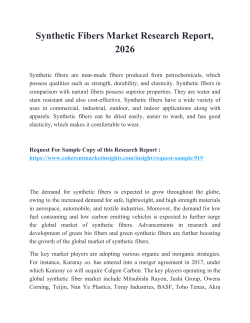
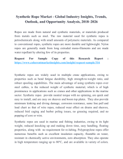
more recent, and some examples of near-IR ts can be found in Bell (1997) and in Figures 1
and 2, which compare our synthetic spectra of the Sun (5780 K, log g = 4.44) and Arcturus
(4350 K, log g = 1.50, [Fe/H] = {0.51, [C/H] = {0.67, [N/H] = {0.44, [O/H] = {0.25,
12 C/13 C = 7) to data taken from spectral atlases of these stars. In each gure, the synthetic
spectra are shown as dotted lines, and the observational data are represented by solid lines;
the former have been calculated at 0.01 A resolution and convolved to the resolution of the
empirical spectra.
The upper panel of Figure 1 shows our synthetic solar spectrum and the ATMOS
spectrum of the Sun (Farmer & Norton 1989) near the bandhead of the 12 CO(4,2) band.
The lower panel of this gure is a similar plot for Arcturus, but the observed spectrum is
taken from NOAO (Hinkle et al. 1995). In Figure 2, NOAO spectra of the Sun (Livingston
& Wallace 1991) and Arcturus (Hinkle et al. 1995) are compared to the corresponding
synthetic spectra in a region of the H band. The NOAO data shown in these two gures
are ground-based and have been corrected for absorption by the Earth's atmosphere. To
allow the reader to judge its importance, the telluric absorption at these wavelengths is
also displayed, in emission and to half-scale, across the bottoms of the appropriate panels;
these telluric spectra have been taken from the same sources as the observational data. The
slight wavelength dierence between the empirical and synthetic spectra in the lower panel
of Figure 1 occurs because the observed spectrum is calibrated using vacuum wavelengths,
while the spectral line lists used to calculate the synthetic spectra assume wavelengths in
air; this oset has been removed in the lower panel of Figure 2.
Note that the oxygen abundance derived for the Sun from the near-infrared vibrationrotation lines of OH is dependent upon the model atmosphere adopted. The Holweger
& Muller (1974) model gives a result 0.16 dex higher than the OSMARCS model of
Edvardsson et al. (1993). We use a logarithmic, solar oxygen abundance of 8.87 dex (on a
scale where H = 12.0 dex), only 0.04 dex smaller than the value inferred from the Holweger
& Muller model. Presumably, this is part of the reason that our CO lines are slightly too
strong in our synthetic solar spectrum while being about right in our synthetic spectrum
of Arcturus (see Figure 1). Overall, though, the agreement between the empirical and
synthetic spectra illustrated in Figures 1 and 2 is typical of that achieved throughout the
{ 10 {
J, H and K bandpasses.
3. The Calculation and Calibration of the Synthetic Colors
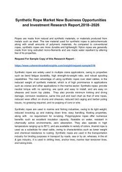
Colors are measured from the synthetic spectra by convolving the spectra with
lter-transmission-proles. To put the synthetic colors onto the respective photometric
systems, we then apply zero-point corrections based upon models of the A-type standard
star, Lyrae (Vega), since the colors of Vega are well-dened in most of these systems.
In this paper, we measure synthetic colors on the following systems using the ltertransmission-proles taken from the cited references { Johnson UBV and Cousins VRI:
Bessell (1990); Johnson-Glass JHK: Bessell & Brett (1988); CIT/CTIO JHK: Persson
(1980); and CIT/CTIO CO: Frogel et al. (1978). Gaussian proles were assumed for the
CO lters. In Figure 3, these lter-transmission-proles overlay our synthetic spectrum of
Arcturus.
The synthetic UBVRI colors are initially put onto the observed Johnson-Cousins system
using the Hayes (1985) absolute-ux-calibration data for Vega. Since Hayes' observations
begin at 3300 A, they must be supplemented by the uxes of a Vega model (9650 K,
log g = 3.90, [Fe/H] = 0.0; Dreiling & Bell 1980) shortward of this. The colors calculated
from the Hayes data are forced to match the observed colors of Vega by the choice of
appropriate zero points; we assume U{B = B{V = 0.0 for Vega and take V{R = {0.009 and
V{I = {0.005, as observed by Bessell (1983). The resulting zero points are then applied to
all of the synthetic UBVRI colors. While this results in UBVRI colors for our Vega model
which are slightly dierent than those observed, we prefer to tie the system to the Hayes
calibration, which is xed, rather than to the Vega model itself because the latter will
change as our modelling improves. The use of our model Vega uxes shortward of 3300 A
introduces only a small uncertainty in the U{B zero points.
Since there is no absolute ux calibration of Vega as a function of wavelength in the
infrared, the VJHK and CO colors are put onto the synthetic system by applying zero
point corrections which force the near-infrared colors of our synthetic spectrum of Vega to
all become 0.0. This is consistent with the way in which the CIT/CTIO and Johnson-Glass
systems are dened by Elias et al. (1982) and Bessell & Brett (1988), respectively.
{ 11 {
3.1. Testing the Synthetic Colors
As a test of our new isochrones and synthetic color calculations, we decided to compare
our 4 Gyr, solar-metallicity isochrone to color-magnitude diagrams (CMDs) of the Galactic
open cluster M67. We chose this cluster because it has been extensively observed and
therefore has a very well-determined age and metallicity. Recent metallicity estimates for
M67 (Janes & Smith 1984, Nissen et al. 1987, Hobbs & Thorburn 1991, Montgomery et al.
1993, Fan et al. 1996) are all solar or slightly subsolar, and the best age estimates of the
cluster each lie in the range of 3{5 Gyr, clustering near 4 Gyr (Nissen et al. 1987, Hobbs
& Thorburn 1991, Demarque et al. 1992, Montgomery et al. 1993, Meynet et al. 1993,
Dinescu et al. 1995, Fan et al. 1996). Thus, we expect this particular isochrone to be a
good match to all of the CMDs of M67.
We translated the theoretical isochrone to the color-magnitude plane by calculating
synthetic spectra for eective temperature/surface gravity combinations lying along it
and then measuring synthetic colors from these spectra. Absolute V-band and K-band
magnitudes were derived assuming MV = +4.84 and BCV = {0.12. After doing this, we
found that our isochrone and the M67 photometry diered systematically in some colors
(see Section 3.2.3), which led us to more closely examine the synthetic color calculations.
By modelling eld stars with relatively well-determined physical properties, we learned that,
after applying the Vega zero-point corrections, some of the synthetic colors were still not on
the photometric systems of the observers. Using these eld star models, we have derived the
linear color calibrations which are needed to put the synthetic colors onto the observational
systems. In the following sections, we describe the derivation of these color calibrations and
show how the application of these relations removes most of the disagreement between the
4 Gyr isochrone and the M67 colors, especially near the main-sequence turno.
Note, however, that the location of the isochrone in the HR diagram does depend upon
the details of the stellar interior calculations, such as the surface boundary conditions and
the treatment of convection, particularly at cooler temperatures. Near the main-sequence
turno, its detailed morphology could also be sensitive to convective overshooting (see
Demarque et al. 1992 and Nordstrom et al. 1997), which we have omitted. The primary
purpose in making comparisons between this isochrone and the M67 photometry is to test
the validity of using this and older isochrones to model the integrated light of galaxies.
;
;
{ 12 {
3.2. The Color Calibrations
It should not be too surprising, perhaps, that the colors measured directly from the
synthetic spectra are not always on the systems dened by the observational data. Bessell
et al. (1998) present an excellent discussion of this topic in Appendix E of their paper. They
conclude that, \As the standard systems have been established from natural system colors
using linear and non-linear corrections of at least a few percent, we should not be reluctant
to consider similar corrections to synthetic photometry to achieve good agreement with the
standard system across the whole temperature range of the models." Thus, we will not
explore why the synthetic colors need to be calibrated to put them onto the observational
systems but instead will focus upon the best way to derive the proper calibrations.
Paltoglou & Bell (1991), BPT94 and Tripicco & Bell (1991) have also looked at the
calibration of synthetic colors. They determined the relations necessary to make the
colors measured from the Gunn & Stryker (1983; hereafter GS83) spectral scans match
the observed photometry of the GS83 stars. This approach has the advantage that it is
model-independent, i.e., it is not tied in any way to the actual spectral synthesis, and should
therefore primarily be sensitive to errors in the lter-transmission-proles. Of course, it is
directly dependent upon the accuracy of the ux calibration of the GS83 scans.
The GS83 scans extend from 3130{10680 A and are comprised of blue and red sections;
these pieces have 20 A and 40 A resolution, respectively, and are joined at about 5750 A.
We have made comparisons of the GS83 scans of stars of similar spectral type and found
the relative ux levels of the blue portions to be very consistent from star to star; however,
there appear to be systematic dierences, often quite large, between the corresponding red
sections. This \wiggle" in the red part of the GS83 scans usually originates near 5750 A, the
point at which the blue and red parts are merged. Because of these discrepancies and other
suspected problems with the ux calibration of the GS83 scans (see e.g., Rufener & Nicolet
1988, Taylor & Joner 1990, Worthey 1994), we have chosen instead to calibrate the synthetic
colors by calculating synthetic spectra of a group of stars which have well-determined
physical properties and comparing the resulting synthetic colors to photometry of these
stars. The drawback of this method is that the calibrations are now model-dependent.
However, since we have decoupled the color calibrations and the GS83 spectra, this allows
us to calibrate both the optical and infrared colors in a consistent manner. In addition,
we use more recent determinations of the photometric lter-transmission-proles than the
previous calibrations cited above.
{ 13 {
3.2.1. Eective Temperature Measurements and the Field Star Sample
To calibrate the synthetic colors, we have chosen a set of eld stars which have
well-determined eective temperatures, since Te is the most critical determinant of stellar
color. Most stars in this set have surface gravity and metallicity measurements as well,
although we have not always checked that the log g and [Fe/H] values were found using
eective temperatures similar to those which we adopt.
The most straightforward way to derive the eective temperature of a star is
through measurement of its angular diameter and apparent bolometric ux. The eective
temperature can then be estimated from the angular diameter through the relation,
!0 25
f
bol
Te / 2
;
(1)
:
where is the limb-darkened angular diameter of the star, hereafter denoted LD, and fbol
is its apparent bolometric ux. Obviously, this method can only be used for nearby stars.
The infrared ux method (IRFM) of Blackwell & Shallis (1977) is regarded as one of
the more reliable ways to estimate Te for stars which are not near enough to have their
angular diameters measured. It relies on the temperature sensitivity of the ratio of the
apparent bolometric ux of a star to the apparent ux in an infrared bandpass (usually
the K band). Model atmosphere calculations are employed to predict the behavior of this
ux ratio with changing Te , and the resulting calibration is then used to infer eective
temperatures from observed uxes. IRFM temperatures have been published by Blackwell
et al. (1990), Blackwell & Lynas-Gray (1994), Saxner & Hammarback (1985; hereafter
SH85), Alonso et al. (1996), and BG89, among others, although BG89 used their color
calculations to adopt nal temperatures which are systematically 80 K cooler than their
IRFM estimates. BG89 also calculated angular diameters for the stars in their sample from
the apparent bolometric uxes that they used in the IRFM and their \adopted" eective
temperatures. We can check the accuracy of these BG89 Te values by comparing their
angular diameter predictions to recent measurements.
Pauls et al. (1997; hereafter PMAHH) have used the U.S. Navy Prototype Optical
Interferometer to make observations in 20 spectral channels between 5200 A and 8500 A
and have measured LD for two of the stars with IRFM temperatures quoted by BG89. In
addition, Mozurkewich et al. (1991) and Mozurkewich (1997) have presented uniform-disk
angular diameters (UD), measured with the Mark III Interferometer at 8000 A, for 20 of
BG89's stars, including the two observed by PMAHH; these data, which we will hereafter
refer to collectively as M97, must be converted to limb-darkened diameters before comparing
them to the other estimates.
{ 14 {
To determine the uniform-disk-to-limb-darkened conversion factor, we performed a
linear, least-squares t between the ratio LD/UD and spectral type for the giant stars
listed in Table 3 of Mozurkewich et al. (1991), using their angular diameters measured at
800 nm. In deriving this correction, And was omitted; LD for And (4.12 mas) does not
follow the trend of the other giants, possibly due to a typographical error (4.21 mas would
t the trend). We applied the resulting limb-darkening correction:
LD =UD = 1:078 + 0:002139 SP ;
(2)
where SP is the spectral type of the star in terms of its M subclass (i.e., SP = 0 for an
M0 star, SP = {1 for a K5 star, etc.), to the M97 angular diameters to derive LD for these
stars, keeping in mind that the predicted correction factor may not be appropriate for all
luminosity classes; for example, the above equation gives LD/UD = 1.033 for CMi, an
F5 IV{V star, while Mozurkewich et al. (1991) used 1.047.
The limb-darkened angular diameters of M97 and PMAHH are compared to the BG89
estimates in Table 1; the M97 and BG89 comparison is also illustrated in Figure 4. Note
that the PMAHH value for UMa is in much better agreement with the BG89 estimate
than is the M97 diameter. The average absolute and percentage dierences between
the BG89 and M97 angular diameters, in the sense BG89 { M97, are only {0.006 mas
and 0.87%, respectively. Translated into eective temperatures, these dierences become
{23 K and 0.44%. For the PMAHH data, the analogous numbers are +0.03 mas (0.51%)
and +13 K (0.30%), albeit for only two stars. This exceptional agreement between the
IRFM-derived and observed angular diameters is a strong conrmation of the \adopted"
eective temperatures of BG89 and gives us faith that any errors in the synthetic colors
which we measure for the stars taken from this source are not dominated by uncertainties
in their eective temperatures.
Since we are condent that the BG89 \adopted" Te scale for giant stars is accurate,
we have used a selection of their stars as the basis of the synthetic color calibrations.
Specically, we chose all of the stars for which they derived IRFM temperatures. However,
BG89 included only G and K stars in their work. For this reason, we have supplemented
the BG89 sample with the F and G dwarfs studied by SH85; before using the latter data,
of course, we must determine whether the IRFM temperatures of SH85 are consistent with
those of BG89.
There is only one star, HR 4785, for which both BG89 and SH85 estimated Te . The
IRFM temperature of SH85 is 5842 K, while BG89 adopt 5861 K. In addition, M97 has
measured an angular diameter for one of the SH85 stars, CMi (HR 2943). Applying
the limb-darkening correction used by Mozurkewich et al. (1991) for this star and using
the bolometric ux estimated by SH85 gives Te = 6569 K; SH85 derive 6601 K. Based
{ 15 {
upon these two stars, it appears that the SH85 eective temperature scale agrees with the
BG89 scale to within 20{30 K, which is well within the expected uncertainties in the
IRFM eective temperatures. Thus, we conclude that the two sets of measurements are in
agreement and adopt the IRFM temperatures of SH85 as given.
Table 2 lists the stars for which we have calculated synthetic spectra for use in
calibrating the synthetic color measurements and gives the eective temperatures, surface
gravities and metallicities used to model each. From BG89, we used the \adopted"
temperatures and metallicities given in their Table 3. In most cases, we used the surface
gravities and metallicities from this table as well. However, for seven of the stars, we
took the more recent log g determinations of Bonnell & Bell (1993a, 1993b). For the
SH85 stars, we assumed the average eective temperatures presented in their Table 7,
omitting stars HR 1008 and HR 2085, which may be peculiar (see SH85); the surface
gravities and metallicities of these stars were taken from Table 5 of SH85. We adopted
the BG89 parameters for HR 4785. For those stars with unknown surface gravities, log g
was estimated from our new isochrones, taking into account the metallicity and luminosity
class of the star, or from other stars of similar eective temperature and luminosity class.
Because most of the stars with well-determined chemical compositions have [Fe/H] 0.0,
solar abundances were assumed for those stars for which [Fe/H] had not been measured.
In Figure 5, we show where the stars used to calibrate the synthetic colors lie in the
log Te , log g plane. Our 3 Gyr and 16 Gyr, solar-metallicity isochrones are also shown in
this gure for reference. Figure 5a shows the entire sample of stars from Table 2; the other
panels present interesting subsets of the larger group. In panels b) and c), the metal-poor
([Fe/H] < {0.3) and metal-rich ([Fe/H] > +0.2) stars are shown, respectively. In panels d),
e) and f), the solar metallicity ({0.3 [Fe/H] +0.2) stars are broken up into the dwarfs
and subgiants (luminosity classes III{IV, IV, IV{V and V), the normal giants (classes II{III
and III), and the brighter giants (classes I and II), respectively.
Even though many of the eld stars in Figure 5a do not t the solar-metallicity
isochrones as well as one might expect, especially along the red-giant branch, examining
the subsets of these stars shows that the \outliers" are mostly brighter giants and/or
metal-poor stars; at a given surface gravity, these stars generally lie at higher temperatures
than the solar-metallicity isochrones, as would be expected from stellar-evolution theory
and observational data. The stars located near log Te = 3.7, log g = 2.7 in panel e) of
Figure 5 (the solar-metallicity giants) are probably clump stars. In fact, there are only
three stars in Figure 5 which lie very far from the positions expected from their physical
properties or spectral classication, and even their locations are not unreasonable. The
three stars in question are represented by lled symbols and are the metal-poor star, Tuc;
{ 16 {
the metal-rich giant, 72 Cyg; and the solar-metallicity giant, 31 Com. Tuc is unusual
in that SIMBAD assigns it the spectral type F1 III, yet it lies very near the turno of
the 3 Gyr, Z isochrone. The Michigan Spectral Survey (Houk & Cowley 1975) classies
this star as an F3 IV{V star, and SH85 listed it as an F-type dwarf, which appears
to be appropriate for its temperature and surface gravity, indicating that the SIMBAD
classication is probably incorrect. 72 Cyg is suspect only because it is hotter than the
solar-metallicity isochrones while having a supersolar metallicity. Since it could simply be
younger (i.e., more massive) than the other stars in the sample, we do not feel justied in
altering the parameters adopted for this star. The third star, 31 Com, lies further from the
isochrones than any other star, but it is classied as a G0 III peculiar star, so perhaps its
log g and Te are not unreasonable either.
Overall, Figure 5 indicates that the temperatures and gravities assigned to the stars in
Table 2 are good approximations to those one would infer from their spectral types and
metallicities.
3.2.2. Derivation of the Color Calibrations
We have calculated a MARCS stellar atmosphere model and an SSG synthetic spectrum
for each of the stars in Table 2. However, rather than compute a separate ODF for each star,
we chose to employ only three ODFs in these model atmosphere calculations { the same
ODFs used in our evolutionary synthesis work (Paper III). For stars with [Fe/H] < {0.3,
a Z = 0.006 ([Fe/H] = {0.46) ODF was used; stars having {0.3 [Fe/H] +0.2 were
assigned a solar-metallicity (Z = 0.01716) ODF; and a Z = 0.03 ([Fe/H] = +0.24) ODF
was used for stars with [Fe/H] > +0.2. The synthetic spectra were then calculated using
the metallicities of the corresponding ODFs.
To calibrate the synthetic colors, photometry of the eld stars in Table 2 has been
compiled from the literature. Since all of these stars are relatively nearby, no reddening
corrections have been applied to this photometry. The UBV photometry comes from
Mermilliod (1991) and Johnson et al. (1966). The VRI data is from Cousins (1980) and
Johnson et al. (1966); the latter were transformed to the Cousins system using the color
transformations of Bessell (1983). The VJHK photometry has been derived from colors
observed on the Johnson system by Johnson et al. (1966), Johnson et al. (1968), Lee
(1970) and Engels et al. (1981) and on the SAAO system by Glass (1974); the color
transformations given by Bessell & Brett (1988) were used to calculate the observed
Johnson-Glass and CIT/CTIO colors. Table 2 cites the specic sources of the photometry
used for each eld star. Unfortunately, we were unable to locate CO observations for a
{ 17 {
sucient number of these stars to be able to calibrate this index.
Although a few colors show a hint that a higher-order polynomial may be superior, we
have t simple linear, least-squares relations to the eld-star data, using the photometric
color as the dependent variable and the synthetic color as the independent variable in each
case and omitting the three coolest dwarfs. Figure 6 shows some of these color-calibration
ts (solid lines), and the zero points and slopes of all of the resulting relations are given
in Table 3; the values listed there are the 1 uncertainties in the coecients of the
least-squares ts. The number of stars used to derive each calibration equation, n, and the
colors spanned by the photometric data are also given in Table 3.
For the optical colors, the coolest dwarfs appear to follow a dierent color calibration
than the other eld stars, so we have also calculated a separate set of color calibrations for
cool dwarfs. This was done by tting a linear relation to the colors of the three reddest eld
dwarfs but forcing this t to intersect the \main" calibration relation of Table 3 at the color
corresponding to a 5000 K dwarf. These cool-dwarf color calibrations are shown as dashed
lines in Figure 6. However, we wish to emphasize that the cool-dwarf color calibrations are
very uncertain, being derived from photometry of only three stars (HR 8085, HR 8086 and
HR 8832); the choice of 5000 K as the temperature at which the cool dwarf colors diverge is
also highly subjective. Thus, since it is not clear to us whether the use of dierent optical
color calibrations for cool dwarfs is warranted, we will proceed by discussing and illustrating
the calibrated colors of the cool dwarf models which result when both the color calibrations
of Table 3 and the separate cool-dwarf calibrations are adopted. In Section 4.1.1, we further
discuss the coolest dwarfs in our sample and possible explanations for their erroneous colors.
Due to the small color range of the H{K photometry and the uncertainties in the
Johnson/SAAO H{K photometry and color transformations, the calibrations derived for
the H{K colors are highly uncertain; application of the corresponding calibrations may
not improve the agreement with the observational data signicantly. It is also apparent
that our U{V calculations are not very good, but we expect them to improve substantially
after the aforementioned Fe I data of Bautista (1997) have been incorporated into both
MARCS and SSG. Additionally, we want to emphasize that the mathematical form of the
color calibrations is presented here only to illustrate their signicance. We caution others
against the use of these specic relations to calibrate synthetic colors in general because the
coecients are dependent, at least in part, on our models.
The poor agreement between the synthetic and observed CIT/CTIO J{K colors,
contrasted with the relatively good t for Johnson-Glass J{K, is probably due to better
knowledge of the J-band lter-transmission-prole of the latter system. This is suggested
by the ratio of the scale factors (slopes) in Table 3 (JG/CIT = 0.976/0.895 = 1.090), which
{ 18 {
is very close to the slope of the color transformation (1.086) between the two systems found
by Bessell & Brett (1988). In other words, our synthetic colors for the two systems are very
similar, while the Bessell & Brett observational transformation indicates that they should
dier.
Even though most of our color calibrations call for only small corrections to the
synthetic colors, we have chosen to apply each of them because every relation has either a
slope or a zero point which is signicant at greater than the 1 level. We believe that using
these calibration equations will help us to reduce the uncertainties in the integrated galaxy
colors predicted by our evolutionary synthesis models (Paper III). Indeed, the importance
of calibrating the synthetic colors when modelling the integrated light of galaxies and other
stellar aggregates becomes apparent when the uncalibrated and calibrated colors of our
4 Gyr, solar-metallicity isochrone are compared to color-magnitude diagrams of M67.
3.2.3. The M67 Color-Magnitude Diagrams
The (uncalibrated) colors of our 4 Gyr, solar-metallicity isochrone were determined by
calculating synthetic spectra for eective temperature/surface gravity combinations lying
along it, measuring synthetic colors from these spectra and then applying the Vega-based
zero-point corrections to these colors. In Figure 7, we show the eects of applying the
color calibrations to the synthetic colors of the 4 Gyr, Z isochrone. In each panel of this
gure, the uncalibrated isochrone is shown as a dotted line, while the calibrated isochrones
are represented by a solid line (Table 3 color calibrations throughout) and a dashed line
(Table 3 relations + cool-dwarf calibrations for optical colors of main-sequence stars cooler
than 5000 K), respectively. The M67 UBVRI photometry of Montgomery et al. (1993) is
shown as small crosses in Figure 7, and the giant-star data tabulated by Houdashelt et al.
(1992) are represented by open circles.
We have corrected the M67 photometry for reddening using E(B{V) = 0.06 and
the reddening ratios of a K star as prescribed by Cohen et al. (1981); we also assumed
E(U{V)/E(B{V) = 1.71. This reddening value is on the upper end of the range of recent
estimates for M67 (Janes & Smith 1984, Nissen et al. 1987, Hobbs & Thorburn 1991,
Montgomery et al. 1993, Meynet et al. 1993, Fan et al. 1996), but we found that a reddening
this large produced the best overall agreement between the 4 Gyr, solar-metallicity isochrone
and the M67 photometry in the region of the main-sequence turno for the complete set of
CMDs which we examined. This reddening leaves the isochrone turno a bit bluer than the
midpoint of the turno-star color distribution in V{I and a bit redder than the analogous
M67 photometry in U{V, but it gives a reasonable t for the other colors. Because the
{ 19 {
turno stars in the MV , U{V CMD suggest a smaller reddening is more appropriate, we also
examined the possibility that the Montgomery et al. (1993) V{I colors are systematically
in error; however, they are consistent with the photometry of M67 reported by Chevalier
& Ilovaisky (1991) and by Joner & Taylor (1990). Most importantly, we simply trust our
synthetic V{I colors (and the corresponding reddening ratios) more than those in U{V,
given the aforementioned uncertainties in the bound-free Fe I opacity, so we accepted the
poorer turno t in the U{V CMD. We derived the absolute magnitudes of the M67 stars,
after correcting for extinction, assuming (m{M)0 = 9.60 (Nissen et al. 1987, Montgomery
et al. 1993, Meynet et al. 1993, Dinescu et al. 1995, Fan et al. 1996).
The agreement between the isochrone and the M67 observations is improved in all of
the CMDs (except perhaps in the H{K diagram, which is not shown) after the isochrone
colors have been calibrated to the photometric systems using the color calibrations derived
in Section 3.2.2. In fact, if we concentrate upon the main-sequence-turno region, there
is no further indication of problems with the synthetic colors, with the possible exception
of U{V, which again is sensitive to opacity uncertainties. The level of agreement between
the photometry and the isochrone along the red-giant branch strengthens this conclusion.
Of course, more R-band and deeper near-infrared photometry of M67 members would be
helpful in verifying this result for the respective colors.
We also note that the detailed t of the isochrone to the M67 turno could possibly
be improved by including convective overshooting in our stellar interior models. While
there is no general agreement regarding the importance of convective overshooting in M67
(see Demarque et al. 1992, Meynet et al. 1993, and Dinescu et al. 1995 for competing
views), solar-metallicity turno stars only slightly more massive than those in M67 do
show evidence for signicant convective overshooting (Nordstrom et al. 1997, Rosvick &
VandenBerg 1998). To help us examine this further, VandenBerg (1999) has provided us
with a 4 Gyr, solar-metallicity isochrone which includes the (small) amount of convective
overshooting which he considers to be appropriate for M67. This isochrone is in excellent
agreement with ours along the lower main-sequence but contains a \hook" feature at the
main-sequence turno, becoming cooler than our 4 Gyr, Z isochrone at MV =3.5 and then
hooking back to be hotter than ours at MV =3.0; this \hook" does appear to t the M67
photometry slightly better. Still, we do not expect convective overshooting to signicantly
aect our evolutionary synthesis models of elliptical galaxies because it will have an even
smaller impact upon the isochrones older than 4 Gyr.
In those colors for which the deepest photometry is available, the calibrated isochrone
is still bluer than the M67 stars on the lower main-sequence when only the color calibrations
of Table 3 are applied. Using separate calibrations for the cool dwarfs makes the faint part
{ 20 {
of the calibrated isochrone agree much better with the U{V and B{V colors of the faintest
M67 stars seen in Figure 7 but appears to overcorrect their V{I colors. This improved t
between the calibrated isochrone and the M67 photometry supports the use of dierent
color calibrations for the optical colors of the cool dwarfs, although there is a hint in
Figure 7 that perhaps the cool-dwarf calibrations should apply at an eective temperature
slightly hotter than 5000 K. Nevertheless, we do not nd lower main-sequence discrepancies
as worrisome as color dierences near the turno would be, since the lowest-mass stellar
interior models are sensitive to the assumed low-temperature opacities, equation of state
and surface pressure boundary treatment. In addition, these faint, lower-main-sequence
stars make only a small contribution to the integrated light of our evolutionary synthesis
models when a Salpeter IMF is assumed. Consequently, small errors in their colors will
not generally have a detectable eect on the integrated light of the stellar population
represented by the entire isochrone.
3.3. Uncertainties in the Synthetic Colors
While the color calibrations are technically appropriate only for stars with near-solar
metallicities, there is no evidence from the photometry of the eld star sample that the
synthetic color calibrations depend upon chemical composition. In fact, it is likely that
we are at least partially accounting for metallicity eects by applying color corrections
as a function of color rather than eective temperature. If the dierences between the
uncalibrated, synthetic colors and the photometry are due to errors in the synthetic
spectra caused by missing opacity, for example, then dierent color corrections would
be expected for two stars having the same temperature but dierent metallicities; the
more metal-poor star should require a smaller correction. This is in qualitative agreement
with the calibrations derived here, since this star would be bluer than its more metal-rich
counterpart.
In this section, we present the sensitivities of the colors to uncertainties in some of
the model parameters: eective temperature, surface gravity, metallicity, microturbulent
velocity ( ) and mixing. We estimate the uncertainties in these stellar properties to be
80 K in Te , 0.3 dex in log g, 0.25 dex in [Fe/H], and 0.25 km s?1 in . To examine
the implications of these uncertainties, we have varied the model parameters of the coolest
dwarf (61 Cyg B), the coolest giant ( Tau) and the hottest solar-metallicity dwarf (HR
4102) listed in Table 2 by the estimated uncertainties, constructing new model atmospheres
and synthetic spectra of these stars. We also constructed an Tau model which neglected
mixing. In Table 4, we present the changes in the uncalibrated synthetic colors which
{ 21 {
result when each of the model parameters is varied as described above. The color changes
presented in this table are the average changes produced by parameter variations in the
positive and negative directions. Since the VJHK color changes were almost always identical
for colors on the Johnson-Glass and CIT/CTIO systems, the (V{K), (J{K) and (H{K)
values given in Table 4 are applicable to either system.
If our uncertainty estimates are realistic, then it is clear from Table 4 that the variations
in most colors are dominated by the uncertainties in one parameter. For the V{R, V{I,
V{K, J{K and H{K colors, this parameter is Te , with the exception being the V{R color
of the cool dwarf, which appears to be especially metallicity-sensitive. The behavior of the
U{V and B{V colors is more complicated. Gravity and metallicity uncertainties dominate
U{V for the cool giant and the hot dwarf, but eective temperature uncertainties have the
greatest inuence on the U{V color of the cool dwarf. Uncertainties in each of the model
parameters have a similar signicance in determining the B{V color of the cool giant,
while those in Te dominate for the cool dwarf, and Te and [Fe/H] uncertainties are most
important in the hot dwarf. Overall, we conclude that estimating the formal uncertainties
of the synthetic colors needs to be done on a star-by-star and color-by-color basis, which
we have not attempted to do. However, it is encouraging to see that Te uncertainties
dominate so many of the color determinations, since our eective temperature scale is
well-established by the angular diameter measurements discussed in Section 3.2.1.
4. The New Color-Temperature Relations and Bolometric Corrections
From the comparisons of the calibrated, 4 Gyr, solar-metallicity isochrone and the
CMDs of M67, we conclude that the color calibrations that were derived in Section 3.2.2
and presented in Table 3 generally put the synthetic colors onto the photometric systems
of the observers but leave some of the optical colors of cool dwarfs too blue. These
calibrations, coupled with the previously described improvements in the model atmospheres
and synthetic spectra, have encouraged us to calculate a new grid of color-temperature
relations and bolometric corrections. The bolometric corrections are calculated after
calibrating the model colors, assuming BCV = {0.12 and MV = +4.84; when coupled
with the calibrated color of our solar model, (V{K)CIT = 1.530, we derive MK = +3.31
and BCK = +1.41. However, keep in mind that the color calibrations have been derived
from Population I stars, so the colors of the models having [Fe/H] <
{0.5 should be used
with some degree of caution (but see Section 3.3).
In Table 5, we present a grid of calibrated colors and K-band bolometric corrections
for stars having 4000 K Te 6500 K and 0.0 log g 4.5 at ve metallicities between
;
;
;
;
{ 22 {
[Fe/H] = {3.0 and solar metallicity; the optical colors of the dwarf (log g = 4.5) models
resulting from the use of the cool-dwarf color calibrations discussed in Section 3.2.2 are
enclosed in parentheses, allowing the reader to decide which color calibrations to adopt
for these models. We will now proceed to compare our new, theoretical color-temperature
relations to empirical relations of eld stars and to previous MARCS/SSG results.
4.1. Comparing Our Results to Other Empirical Color-Temperature Relations
In the following sections, we use the photometry and eective temperatures of the stars
listed in Table 2 to derive empirical color-temperature relations for eld giants and eld
dwarfs. We then compare our models and our empirical, solar-metallicity color-temperature
relations to the CT relations of eld stars which have been derived by Blackwell &
Lynas-Gray (1994; hereafter BLG94), Gratton et al. (1996; hereafter GCC96), Bessell
(1979; hereafter B79), Bessell (1995; hereafter B95), Bessell et al. (1998; hereafter BCP98)
and Bessell (1998; hereafter B98).
4.1.1. The Color-Temperature Relations of Our Field Stars
The color and temperature data for our set of color-calibrating eld stars are plotted
in Figures 8 and 9, where we have split the sample into giants (log g 3.6) and dwarfs
(log g > 3.6), shown in the lower and upper panels of the gures, respectively. We have
t quadratic relations to the eective temperatures of the dwarfs and giants separately
as a function of color to derive empirical, solar-metallicity color-temperature relations for
each; the resulting CT relations of the giants and dwarfs are shown as bold, solid lines and
bold, dotted lines, respectively, in these gures. The coecients of the ts (and their 1
uncertainties) are given in Table 6. The calibrated colors of our M67 isochrone (4 Gyr, Z)
are also plotted in Figures 8 and 9 as solid lines; the dashed lines in the upper panels of
Figure 8 show the calibrated isochrone when the cool-dwarf color calibrations are applied.
Comparisons with our other isochrones indicate that the CT relation of the solar-metallicity
isochrones is not sensitive to age.
Although we have divided our eld-star sample into giants and dwarfs, the empirical
CT relations of the two groups only appear to dier signicantly in (V{R)C and (V{I)C.
In B{V and J{K, the CT relations of the dwarfs and giants are virtually identical, and it
is only the color of the coolest dwarf that prevents the same from being true in V{K. The
dierences in the U{V color-temperature relations of the dwarfs and giants can largely be
{ 23 {
attributed to the manner in which we chose to perform the least-squares tting. Therefore,
we want to emphasize that our tabulation of separate CT relations for dwarfs and giants
does not necessarily infer that the two have signicantly dierent colors at a given Te .
It is apparent that the calibrated isochrone matches the properties of the eld giants
very nicely in Figures 8 and 9 and, in fact, is usually indistinguishable from the empirical
CT relation. However, using the color calibrations of Table 3, the dwarf and giant portions
of the isochrone diverge cooler than 5000 K in all colors; this same behavior is not always
seen in the stellar data. This discrepancy at cool temperatures means that one of the
following conditions must apply: 1) the eld star eective temperatures of the cool dwarfs
are systematically too hot; 2) the isochrones predict the wrong Te /gravity relation for
cool dwarfs; or 3) the cool dwarf temperatures and gravities are correct but the model
atmosphere and/or synthetic spectrum calculations are wrong for these stars. Only the
latter condition would lead to dierent color calibrations being required to put the colors of
cool dwarfs and cool giants onto the photometric systems.
The previously-mentioned comparison between our isochrones and those of VandenBerg
(1999) lead us to believe that the lower main-sequence of our 4 Gyr, solar-metallicity
isochrone is essentially correct, so it would appear that the synthetic colors of the coolest
dwarf models are bluer than the color calibrations of Table 3 would predict because either
we have adopted incorrect eective temperatures for these stars or there is some error in
the model atmosphere or synthetic spectrum calculations, such as a missing opacity source.
Unpublished work on CO band strengths in cool dwarfs suggests that part of the
problem could lie with the BG89 temperatures derived for these stars. In addition, some
IRFM work (Alonso et al. 1996) indicates that the eective temperatures adopted for
our K dwarfs cooler than 5200 K may be too hot by 100 K and infers an even larger
discrepancy (up to 400 K) for HR 8086. A recent angular diameter measurement (Pauls
1999) also predicts a hotter Te than we adopted for HR 1084. If our K-dwarf eective
temperatures are too warm, this would imply that the cool-dwarf color calibrations should
not be used because the errors lie in the model parameters adopted for the cool dwarfs
and not in the calculation of their synthetic spectra. However, Te errors of 100 K are not
suciently large to make the three cool eld dwarfs lie on the optical color calibrations of the
other stars (see Table 4). In addition, the similarities of the V{K and J{K colors of our two
coolest dwarfs and those of the calibrated isochrone at the assumed eective temperatures
argue that the Te estimates are essentially correct but do not preclude temperature changes
of the magnitude implied by the IRFM and angular diameter measurements. Thus, some
combination of Te errors and model uncertainties may conspire to produce the color eects
seen here, and more angular diameter measurements of K dwarfs would be very helpful
{ 24 {
in sorting out these possibilities. Nevertheless, the use of the cool-dwarf color calibrations
improves the agreement between the models and the empirical data so remarkably well in
Figures 7 and 8 that a good case can be made for their adoption.
As discussed in the Section 3.3, the model B{V colors of giants are noticeably dependent
on gravity at low temperatures. The agreement between the observed B{V colors and the
corresponding calibrated, synthetic colors for both the sample of eld stars and the cool
M67 giants suggests that the gravity-temperature relation of the isochrone truly represents
the eld stars, even at cool temperatures. While this is certainly anticipated, the fact that
it occurs indicates that the surface boundary conditions and mixing-length ratio used for
the interior models are satisfactory and gives us condence that these newly-constructed
isochrones are reasonable descriptions of the stellar populations they are meant to represent
in our evolutionary synthesis program.
4.1.2. Other Field-Star Color-Temperature Relations
BLG94 estimated eective temperatures for 80 stars using the IRFM and derived V{K,
Te relations for the single stars, known binaries and total sample which they studied.
Because these three relations are very similar, we have adopted their single star result for
our comparisons, after converting their V{K colors from the Johnson to the Johnson-Glass
system using the color transformation given by Bessell & Brett (1988). We expect the
BLG94 eective temperature scale to be in good agreement with that adopted here for the
eld stars used to derive the color calibrations { for the 19 stars in common between BLG94
and BG89, BLG94 report that the average dierence in Te is 0.02%. For later discussion,
we note that the coolest dwarf included in BLG94's sample is BS 1325, a K1 star, with
Te = 5163 K.
GCC96 derived their CT relations from photometry of about 140 of the BG89 and
BLG94 stars. They adjusted BG89's IRFM Te estimates to put them onto the BLG94
scale and then t polynomials to the eective temperatures as a function of color to
determine CT relations in Johnson's B{V, V{R2, R{I, V{K and J{K colors. In each color,
they derived three relations { one represents the dwarfs, and the other two apply to giants
bluer and redder than some specic color. For these relations, we have used B79's color
transformations to convert the Johnson V{R and V{I colors to the Cousins system; Bessell
& Brett (1988) again supplied the V{K and J{K transformations to the Johnson-Glass
2 Gratton (1998) has advised us that the a3 coecient of the Te , V{R relation of the bluer class III stars
should be +85.49; it is given as {85.49 in Table 1 of GCC96.
{ 25 {
system.
BCP98 combined the IRFM eective temperatures of BLG94 and temperatures
estimated from the angular diameter measurements of di Benedetto & Rabbia (1987), Dyck
et al. (1996) and Perrin et al. (1998) to derive a polynomial relation between V{K and
Te for giants. The color-temperature relations provided by B98 are presumably derived
in exactly the same manner from this same group of stars. For cool dwarfs, BCP98 also
determined a CT relation, this time in V{I, from the IRFM eective temperatures of
BLG94 and Alonso et al. (1996).
B79 merged his V{I, V{K color-color relation for eld giants and the V{K, Te relation
of Ridgway et al. (1980) to come up with a V{I, Te relation. He then combined this
with V{I, color trends to dene CT relations for giants in other colors. By assuming that
the same V{I, Te relation applied to giants and dwarfs with 4000 K Te 6000 K,
B79 derived dwarf-star CT relations in a similar manner. For the coolest dwarfs, updated
versions of B79's V{R, Te and V{I, Te relations were given by B95.
4.1.3. Comparisons of the Color-Temperature Relations
We compare our calibrated, solar-metallicity color grid to empirical determinations of
color-temperature relations of eld stars in Figures 10{14. For these comparisons, we break
our grid up into giants & subgiants, which we equate with models having 0.0 log g 4.0,
and dwarfs (log g = 4.5). In all of the gures in this section, the giant-star CT relations
appear in the upper panels, and the lower panels give the dwarf relations. The calibrated
colors of our solar-metallicity grid are shown as open circles (or as asterisks when the
cool-dwarf color calibrations have been used), but to relieve crowding in the giant-star plots,
we connect the model colors at a given Te by a solid line and plot only the highest and
lowest gravity models as open circles. Our empirical color-temperature relations (Table 6)
are shown as solid lines in Figures 10{14; the CT relations taken from the literature
are represented by the symbols indicated in the gures. In addition, our calibrated,
solar-metallicity, 4 Gyr isochrone is shown as a dotted line; the dashed line in the dwarf-star
panels of Figures 10{12 is the calibrated isochrone which results when the cool-dwarf color
calibrations have been used. Comparisons with our other solar-metallicity isochrones shows
that this CT relation is insensitive to age, so it should agree closely with the eld-star
relations. We omit the U{V and H{K color-temperature relations from these comparisons
because we are not aware of any recent determinations of eld-star relations in these colors,
which nevertheless are less well-calibrated than the others.
{ 26 {
For the giant stars, our empirical CT relations are in excellent agreement with the eld
relations of BLG94, GCC96, BCP98 and B98, with the temperature dierences at a given
color usually much less than 100 K. The 4 Gyr, Z isochrone also matches the eld-giant
relations quite well, as would be expected from Figures 8 and 9. In fact, most of the (small)
dierences between our empirical CT relations and the isochrone are probably due to our
decision to use quadratic relations to represent the eld stars; a quadratic function may
not be a good representation of the true color-temperature relationships, and such a t
often introduces a bit of excess curvature at the color extremes of the observational data.
The B79 color-temperature relations for giants are also seen to be in good agreement with
the other empirical and theoretical, giant-star data in V{R and V{I, but his B{V, Te
relation is bluer than the others; we have not attempted to determine the reason for this
discrepancy.
Overall, since the colors of the eld giants lie within the bounds of our solar-metallicity
grid at a given eective temperature and also show good agreement with the 4 Gyr
isochrone, our calibrated models are accurately reproducing the colors of solar-metallicity,
F{K eld giants of a specic temperature and surface gravity. Unfortunately, the dwarf-star
color-temperature relations do not show the same level of agreement as those of the giants,
overlying one another for Te >
5000 K but diverging at cooler eective temperatures.
Therefore, we will examine each of the CT relations of the dwarfs individually.
In B{V (Figure 10), the eld stars from Table 2 produce a CT relation which is in good
agreement with that of GCC96. When using the color calibrations of Table 3, our isochrone
and grid models of cool dwarfs are bluer than the empirical relations at a given Te , which
is consistent with the comparison to M67 in Figure 7, indicating that these calibrated B{V
colors are too blue. On the other hand, the agreement between these models and the CT
relation of B79 suggests that these grid and isochrone colors are essentially correct. Similar
quandaries are posed by the color-temperature relations of the dwarfs in V{R and V{I
(Figures 11 and 12). Here, the B79 relations predict slightly bluer colors than the analogous
isochrone and grid models at a given temperature, but B95's updated data for the coolest
dwarfs agrees with our calibrated isochrone and models quite well. Our empirical CT
relations for dwarfs and the GCC96 data, on the other hand, lie to the red of these models
and isochrones, again showing the same kind of discrepancy seen in the M67 comparisons.
Unfortunately, the BCP98 V{I, Te relation does not extend to cool enough temperatures
to help resolve the situation. Supplementing the color calibrations of Table 3 with the
(optical) cool-dwarf color calibrations, however, brings the solar-metallicity isochrone and
models into agreement with all of the eld-dwarf CT relations of GCC96 instead.
In Figure 13, we also see that there is one empirical CT relation (BLG94) which
{ 27 {
indicates that our cool-dwarf models are essentially correct at a given Te , while another
(GCC96) predicts that they are too blue, although the magnitude of disagreement in this
gure is much smaller than that seen in Figures 10{12. Since we are not aware of any
near-infrared photometry for lower-main-sequence stars in M67, we cannot use Figure 7 to
bolster any of the V{K CT relations. The only color in which all of the theoretical and
empirical data are in relative agreement for the dwarfs is J{K; this is shown in Figure 14.
We hesitate to emphasize the similarities between our empirical color-temperature
relations and the others plotted in the dwarf-star panels of Figures 10{14. Our V{K CT
relation for eld stars only diers from that of BLG94 because they neglected to treat
dwarfs and giants separately; if we do the same, these dierences disappear. Even so,
the coolest dwarf in the BLG94 study was BS 1325, a K1 V star with Te = 5163 K,
which is hotter than the temperature at which the dwarf and giant CT relations begin
to bifurcate, so it is somewhat misleading to extend BLG94's relation to redder colors in
the dwarf-star panel of Figure 13. Likewise, it is not surprising that our CT relations and
GCC96's relations are so compatible { GCC96 used the BLG94 and BG89 data to dene
their relations, so the cool end of their dwarf relations are dened by the same cool dwarfs
included in our sample. The poor agreement between the other empirical CT relations and
the dwarf-star relations of B79 is probably due to the manner in which B79 derived his
eld-star relations. He assumed a similar V{I, Te relation for cool dwarfs and cool giants,
an assumption which Figure 8 suggests to be inappropriate.
Overall, then, if we assume that the eective temperatures and photometry that we
have adopted for the eld stars of Table 2 and the members of M67 are all correct, we can
account for the similarities and the dierences between our color-temperature relations and
those taken from the literature. In this case, it appears that the CT relations of GCC96
are the most representative of eld dwarfs, while each of those which we have examined
are probably equally reliable for the eld giants (except B79's B{V, Te relation). This
also produces a consistent picture in which both the eld-star CT relations and the M67
photometry indicate that our model colors for cool dwarfs are too blue at a given eective
temperature if only the color calibrations of Table 3 are employed; adopting the cool-dwarf
color calibrations for Te < 5000 K then brings the models and the observational data into
close agreement.
However, we can envision an alternate scenario in which the coolest three (or more)
eld dwarfs have been assigned eective temperatures which are too hot. By lowering Te
by 100 K for HR 8085 and HR 8832 and by 200 K for HR 8086, these stars would lie
along the the same color calibrations as the other eld stars in all colors except perhaps
U{V and B{V. This would shift our empirical CT relations and those of GCC96 to bluer
{ 28 {
colors for the cool dwarfs and thus resolve the disagreement with B95's relations and the
models calibrated using the Table 3 color calibrations. It would also leave V{R and V{I as
the only two colors in which the dwarf-star and giant-star CT relations dier signicantly,
which is understandable, since the V, R and I bands contain many molecular features (e.g.,
TiO, CN) which are gravity-sensitive. However, the discrepancies between the calibrated,
4 Gyr, solar-metallicity isochrone (solid line in Figure 7) and the U{V and B{V photometry
of the lower main-sequence of M67 would likely remain.
Since it is not clear to us which of these situations applies, we have presented the
calibrated model colors for each case here. The essential pieces of information needed to
disentangle these two possibilities are angular diameter measurements of K dwarfs; these
would certainly aid us in testing the BG89 temperatures of the cool dwarfs in our sample
and conrming their CT relations. However, for the time-being, the small number of cool
dwarfs with eective temperature estimates and the fact that such stars make only a small
contribution to the integrated light of a galaxy have led us to adopt the calibration relations
given in Table 3 for the synthetic colors of all of our evolutionary synthesis models.
4.2. Comparisons to Previous MARCS/SSG Color-Temperature Relations
In Figures 15 and 16, we compare our new, solar-metallicity CT relations to the
previous MARCS/SSG results published by VB85 and BG89; the models of the former
and latter are shown as open and lled circles, respectively. In each panel of these gures,
we plot log g vs. color and use dotted lines to represent isotherms resulting from the
uncalibrated colors of our models; the isotherms produced by our improved, calibrated
colors (Table 3 calibrations only) are shown as solid lines. Thus, dierences between the
older colors and the appropriate dotted line can be identied with improvements in the
models and color measurements, and dierences between the dotted and solid lines of the
same temperature can be equated with the eects of calibrating the synthetic colors.
4.2.1. The Optical Color-Temperature Relations
In the upper panel of Figure 15, we compare our CT relations and the B{V colors
calculated by VB85 using the lter-transmission-proles of Matthews & Sandage (1963).
The calibrated B{V colors are always redder than their previous counterparts, but the
uncalibrated colors of the new models do not dier appreciably from those of VB85 for
Te >
5000 K; the main improvement in the B{V colors of these hotter stars is due to the
{ 29 {
color calibrations. At 4500 K, especially as log g decreases, the improved low-temperature
opacity data used here becomes important, and this becomes the dominant improvement
for cooler stars, although the color corrections inferred from the calibrations are still
substantial.
The V{R colors of VB85 and BG89, measured with the R-band lter of Cousins (1980),
are compared to our new, solar-metallicity color grid in the middle panel of Figure 15.
Surprisingly, for eective temperatures hotter than about 5000 K, the colors of the older
models are in good agreement with those of the newer, calibrated models; either the color
dierences produced by the lter-transmission-proles adopted by each group are being
almost exactly oset by the eects of the color calibrations which we have derived, or the
newer opacities used here have moved the V{R colors of the models to the blue. For the cool
giants, however, the calibrated V{R colors are signicantly redder than those previously
published.
For V{I, the new and old models are shown in the lower panel of Figure 15. This
diagram is similar to the V{R plot in that it is dicult to disentangle the color changes
produced by the use of dierent lter proles (VB85 and BG89 use the I-band lter
of Cousins 1980) and those resulting from improvements in the stellar modelling. It
is apparent, however, that the previous MARCS/SSG V{I colors are too red at hotter
temperatures (Te >
5500 K) and too blue at cooler temperatures.
4.2.2. The Near-Infrared Color-Temperature Relations
Figure 16 (upper panel) shows that the synthetic V{K colors on the CIT/CTIO
system are not altered appreciably by calibration, at least with respect to the color
range of the models and the magnitude of the color dierences which exist between the
newer and older models. While the colors of our models and those of BG89 are about
the same at Te = 4500 K, the newer models are redder at temperatures cooler than
this and the older models are redder at hotter temperatures. Dierences in the model
atmospheres and synthetic spectra are responsible for these eects, since BG89 used the
same lter-transmission-proles that we have.
The CIT/CTIO J{K colors shown in the lower panel of Figure 16 are all signicantly
bluer than those previously published. For the hotter models, improvements in MARCS and
the much better treatment of line absorption in SSG are the major causes of these blueward
shifts. In fact, the magnitude of the color dierences between the older colors and the newer,
uncalibrated colors is about the same at all temperatures. The color calibrations, however,
{ 30 {
while also making the model J{K colors bluer, grow in importance as Te decreases; this
eect begins to dominate the color shifts due to the model improvements at Te 4500 K.
5. Conclusion
We have calculated colors and bolometric corrections for grids of stellar models having
4000 Te 6500 K, 0.0 log g 4.5 and {3.0 [Fe/H] 0.0. The synthetic colors
which we measure include Johnson U{V and B{V; Cousins V{R and V{I; Johnson-Glass
V{K, J{K and H{K; and CIT/CTIO V{K, J{K, H{K and CO. These synthetic colors have
been determined by convolving the most recent estimates of the lter-transmission-proles
of the respective photometric systems with newly-calculated synthetic spectra. The
synthetic spectra are produced by the SSG spectral synthesis code, which has been updated
signicantly, especially in terms of its low-temperature opacity data and spectral line lists.
The MARCS model atmospheres which are used by SSG have also been calculated using
this new opacity data and improved opacity distribution functions.
We have found that the initial synthetic colors require small corrections to be put
onto the observational systems. Here, we have assembled a set of eld stars which have
eective temperatures measured using the infrared-ux method (IRFM), and we have used
photometry of these stars to derive the color calibrations needed to put the synthetic colors
onto the photometric systems. The scale factors and zero points of these calibrations are
gratifyingly close to unity and small, respectively, but the UBVRI colors of the coolest
dwarfs (Te < 5000 K) may require a more substantial correction. Nevertheless, the specic
color calibrations which we adopt are only applicable to models calculated with our versions
of the MARCS and SSG computer codes. We encourage others to examine the need for
such calibrations in their models as well.
Using the eld-star data adopted in deriving the color calibrations, we have also found
that the recent angular diameter measurements of Mozurkewich et al. (1991), Mozurkewich
(1997) and Pauls et al. (1997) match the angular diameters predicted by Bell & Gustafsson
(1989) very well, thus giving strong conrmation of the latter's eective temperature scale,
which we have adopted. Since most of the synthetic colors are much more sensitive to
eective temperature than they are to the other model parameters, such as metallicity and
surface gravity, this infers that the dierences between the uncalibrated, synthetic colors
and the eld-star photometry are not caused by errors in the temperatures of the eld-star
models. The coolest eld dwarfs may again prove an exception to this generalization, as
none of their angular diameters have been measured and their eective temperatures are
therefore more uncertain. Knowing that the IRFM-derived temperatures are accurate has
{ 31 {
also allowed us to determine empirical, color-temperature (CT) relations for these eld F{K
stars.
After calibrating our synthetic colors, our newly-calculated, 4 Gyr, Z isochrone is seen
to be in good agreement with optical and near-infrared color-magnitude diagrams of M67
from the upper main-sequence through the tip of the red-giant branch. For giants and for
dwarfs hotter than about 5000 K, our theoretical, solar-metallicity CT relations and solarmetallicity isochrones are also found to match the empirical, eld-star color-temperature
relations derived here and found elsewhere in the literature. For the coolest dwarfs (Te <
5000 K), there are some dierences between our empirical color-temperature relations and
the best-determined relations of others. The calibrated colors of the cool-dwarf models also
remain a bit bluer than the eld-star relations (at a given Te ) and the M67 main-sequence
stars (at a given absolute magnitude). Because we have not been able to determine whether
the synthetic, optical colors of the cool dwarf models are too blue because their adopted
eective temperatures are too hot or the synthetic spectra are in error, we present alternate
UBVRI colors for our models having Te < 5000 K and log g = 4.5. These colors are based
upon separate color calibrations derived from only the cool eld dwarfs and which greatly
improve the agreement between the calibrated, synthetic colors and the empirical data. We
leave it to the reader to decide which model colors they prefer.
This work would greatly benet from further eective temperature estimates of cool
dwarfs and measurements of the corresponding angular diameters needed to conrm them.
It would also be quite useful to acquire additional photometry of the eld stars used here
to derive the color calibrations. Only a small subset of these stars, which includes no
cool dwarfs, has been observed on the Cousins system, making the V{R and V{I color
calibrations less well-determined than some of the others. In addition, only Johnson
near-infrared photometry was available for the eld stars. Color transformations had to
be applied to this photometry before the Johnson-Glass and CIT/CTIO color calibrations
could be derived; this also prohibited the determination of a similar calibration for the
CIT/CTIO CO index.
Overall, the agreement between our theoretical CT relations and the empirical data
and between our 4 Gyr, solar-metallicity isochrone and the photometry of M67 indicates
that our synthetic spectra are generally providing a good representation of the spectral
energy distributions of stars of the corresponding Te , surface gravity and metallicity. This
conclusion is further supported by our synthetic spectra of M giants, which are presented
in a companion paper (Houdashelt et al. 2000). In a future paper (Houdashelt et al. 2001),
we will use similar synthetic spectra and newly-constructed isochrones as part of a program
to simulate the spectral energy distributions of early-type galaxies through evolutionary
{ 32 {
synthesis.
We would like to thank the National Science Foundation (Grant AST93-14931) and
NASA (Grant NAG53028) for their support of this research. We also thank Ben Dorman
for allowing us to use his isochrone-construction code and Mike Bessell for providing many
helpful suggestions on the manuscript. MLH would like to express his gratitude to Rosie
Wyse for providing support while this work was completed. The research has made use of
the Simbad database, operated at CDS, Strasbourg, France. The NSO/Kitt Peak FTS data
used here were produced by NSF/NOAO.
REFERENCES
Alonso, A., Arribas, S., & Martinez-Roger, C. 1996, A&AS, 117, 227
Azusienis, A., & Straizys, V. 1969, Soviet Astron. J., 13, 316
Balachandran, S. C., & Bell, R. A. 1998, Nature, 392, 791
Bautista, M. A. 1997, A&AS, 122, 167
Bell, K. L., & Berrington, K. A. 1987, J. Phys. B, 20, 801
Bell, K. L., Kingston, A. E., & McIlveen, W. A. 1975, J. Phys. B, 8, 659
Bell, R. A. 1997, in IAU Symp. 189, Fundamental Stellar Properties: The Interaction
Between Observation and Theory, ed. T. R. Bedding, A. J. Booth, & J. Davis
(Dordrecht: Kluwer), 159
Bell, R. A., Dwivedi, P. H., Branch, D., & Huaker, J. N. 1979, ApJS, 41, 593
Bell, R. A., Eriksson, K., Gustafsson, B., & Nordlund, A. 1976, A&AS, 23, 37
Bell, R. A., & Gustafsson, B. 1978, A&AS, 34, 229 (BG78)
Bell, R. A., & Gustafsson, B. 1989, MNRAS, 236, 653 (BG89)
Bell, R. A., Paltoglou, G., & Tripicco, M. J. 1994, MNRAS, 268, 771 (BPT94)
Bell, R. A., & Tripicco, M. J. 1995, in ASP Conf. Ser. 78, Astrophysical Applications of
Powerful New Databases, ed. S. J. Adelman, & W. L. Wiese (San Francisco: ASP),
365
{ 33 {
Bergbusch, P. A., & VandenBerg, D. A. 1992, ApJS, 81, 163
Bessell, M. S. 1979, PASP, 91, 589 (B79)
Bessell, M. S. 1983, PASP, 95, 480
Bessell, M. S. 1990, PASP, 102, 1181
Bessell, M. S. 1995, in The Bottom of the Main Sequence { And Beyond, ed. C. Tinney
(Berlin: Springer-Verlag), 123 (B95)
Bessell, M. S. 1998, private communication (B98)
Bessell, M. S., & Brett, J. M. 1988, PASP, 100, 1134
Bessell, M. S., Castelli, F., & Plez, B. 1998, A&A, 333, 231 (BCP98)
Biemont, E., Brault, J. W., Delbouille, L., & Roland, G. 1985a, A&AS, 61, 107
Biemont, E., Brault, J. W., Delbouille, L., & Roland, G. 1985b, A&AS, 61, 185
Biemont, E., Brault, J. W., Delbouille, L., & Roland, G. 1986, A&AS, 65, 21
Blackwell, D. E., & Lynas-Gray, A. E. 1994, A&A, 282, 899 (BLG94)
Blackwell, D. E., Petford, A. D., Arribas, S., Haddock, D. J., & Selby, M. J. 1990, A&A,
232, 396
Blackwell, D. E., & Shallis, M. J. 1977, MNRAS, 180, 177
Bonnell, J. T., & Bell, R. A. 1993a, MNRAS, 264, 319
Bonnell, J. T., & Bell, R. A. 1993b, MNRAS, 264, 334
Briley, M. M., Hesser, J. E., Bell, R. A., Bolte, M., & Smith, G. H. 1994, AJ, 108, 2183
Buser, R., & Kurucz, R. L. 1992, A&A, 264, 557
Charbonnel, C. 1994, A&A, 282, 811
Charbonnel, C. 1995, ApJ, 453, L41
Charbonnel, C., Brown, J. A., & Wallerstein, G. 1998, A&A, 332, 204
Chevalier, C., & Ilovaisky, S. A. 1991, A&AS, 90, 225
Cohen, J. G., Frogel, J. A., Persson, S. E., & Elias, J. H. 1981, ApJ, 249, 481
{ 34 {
Cousins, A. W. J. 1980, South African Astron. Obs. Circ., 1, 234
Davis, D. S., Andrew, K. L., & Verges, J. 1978, J. Opt. Soc. Am., 68, 235
Delbouille, L., Roland, G., & Neven, L. 1973, Photometric Atlas of the Solar Spectrum from
3000 to 10000, Institut d'Astrophysique de l'Universite de Liege, Observatoire
royal de Belgique
Demarque, P., Green, E. M., & Guenther, D. B. 1992, AJ, 103, 151
Di Benedetto, G. P., & Rabbia, Y. 1987, A&A, 188, 114
Dinescu, D. I., Demarque, P., Guenther, D. B., & Pinsonneault, M. H. 1995, AJ, 109, 2090
Doughty, N. A., & Fraser, P. A. 1966, MNRAS, 132, 267
Dragon, J. N., & Mutschlecner, J. P. 1980, ApJ, 239, 1045
Dreiling, L. A., & Bell, R. A. 1980, ApJ, 241, 736
Dyck, H. M., Benson, J. A., van Belle, G. T., & Ridgway, S. T. 1996, AJ, 111, 1705
Edvardsson, B., Andersen, J., Gustafsson, B., Lambert, D. L., Nissen, P. E., & Tomkin, J.
1993, A&A, 275, 101
Elias, J. H., Frogel, J. A., Matthews, K., & Neugebauer, G. 1982, AJ, 87, 1029
Engels, D., Sherwood, W. A., Wamsteker, W., & Schultz, G. V. 1981, A&AS, 45, 5
Fan, X., Burstein, D., Chen, J.-S., Zhu, J., Jiang, Z., Wu, H., Yan, H., Zheng, Z., Zhou, X.,
Fang, L.-Z., Chen, F., Deng, Z., Chu, Y., Hester, J. J., Windhorst, R. A., Li, Y., Lu,
P., Sun, W.-H., Chen, W.-P., Tsay, W.-S., Chiueh, T.-H., Chou, C.-K., Ko, C.-M.,
Lin, T.-C., Guo, H.-J., & Byun, Y.-I. 1996, AJ, 112, 628
Farmer, C. B., & Norton, R. H. 1989, A High-Resolution Atlas of the Infrared Spectrum of
the Sun and the Earth Atmosphere from Space, Vol. I: The Sun (NASA RP-1224)
(Washington: NASA)
Forsberg, P. 1991, Phys. Scr, 44, 446
Frogel, J. A., Persson, S. E., Aaronson, M., & Matthews, K. 1978, ApJ, 220, 75
Geller, M. 1992, A High-Resolution Atlas of the Infrared Spectrum of the Sun and the
Earth Atmosphere from Space, Vol. III: Key to Identication of Solar Features
(NASA RP-1224) (Washington: NASA)
{ 35 {
Gilroy, K. K., & Brown, J. A. 1991, ApJ, 371, 578
Glass, I. S. 1973, MNRAS, 164, 155
Glass, I. S. 1974, Mon. Notes Astron. Soc. South Africa, 33, 53
Goorvitch, D. 1994, ApJS, 95, 535
Gratton, R. G. 1998, private communication
Gratton, R. G., Carretta, E., & Castelli, F. 1996, A&A, 314, 191 (GCC96)
Grevesse, N., & Noels, A. 1993, in Origin and Evolution of the Elements, ed. N. Pratzo, E.
Vangioni-Flam, & M. Casse (Cambridge: Cambridge), 15
Gunn, J. E., & Stryker, L. L. 1983, ApJS, 52, 121 (GS83)
Gustafsson, B., & Bell, R. A. 1979, A&A, 74, 313
Gustafsson, B., Bell, R. A., Eriksson, K., & Nordlund, A. 1975, A&A, 42, 407
Hayes, D. S. 1985, in IAU Symp. 111, Calibration of Fundamental Stellar Quantities, ed.
D. S. Hayes, L. E. Pasinetti, & A. G. D. Philip (Dordrecht: Reidel), 225
Henyey, K., Vardya, M. S., & Bodenheimer, P. 1965, ApJ, 142, 841
Hinkle, K., Wallace, L., & Livingston, W. 1995, PASP, 107, 1042
Hobbs, L. M., & Thorburn, J. A. 1991, AJ, 102, 1070
Holweger, H. 1970, A&A, 4, 11
Holweger, H., & Muller, H. A. 1974, Sol. Phys., 39, 19
Houdashelt, M. L., Frogel, J. A., & Cohen, J. G. 1992, AJ, 103, 163
Houdashelt, M. L., Bell, R. A., & Sweigart, A. V. 2001, in preparation (Paper III)
Houdashelt, M. L., Bell, R. A., Sweigart, A. V., & Wing, R. F. 2000, AJ, accepted
(Paper II)
Houk, N., & Cowley, A. P. 1975, Michigan Catalogue of Two-Dimensional Spectral Types
for the HD Stars, Vol. 1 (Ann Arbor: Univ. Michigan Dept. Astron.)
Janes, K. A., & Smith, G. H. 1984, AJ, 89, 487
{ 36 {
Johansson, S., & Learner, R. C. M. 1990, ApJ, 354, 755
Johnson, H. L. 1965, ApJ, 141, 923
Johnson, H. L., MacArthur, J. W., & Mitchell, R. I. 1968, ApJ, 152, 465
Johnson, H. L., Mitchell, R. I., Iriarte, B., & Wisniewski, W. Z. 1966, Comm. Lun. Plan.
Lab, 4, 99
Joner, M. D., & Taylor, B. J. 1990, PASP, 102, 1004
Kjrgaard, P., Gustafsson, B., Walker, G. A. H., & Hultqvist, L. 1982, A&A, 115, 145
Kurucz, R. L. 1991, in Stellar Atmospheres: Beyond Classical Models, ed. L. Crivellari, I.
Hubeny, & D. G. Hummer (NATO ASI Ser. C, 341) (Dordrecht: Kluwer), 408
Kurucz, R. L., van Dishoeck, E. F., & Tarafdar, S. P. 1987, ApJ, 322, 992
Lee, T. A. 1970, ApJ, 162, 217
Litzen, U., Brault, J. W., & Thorne, A. P. 1993, Phys. Scr, 47, 628
Livingston, W., & Wallace, L. 1991, An Atlas of the Solar Spectrum in the Infrared from
1850 to 9000 cm?1 (1.1 to 5.4 microns) (N.S.O. Technical Report #91-001, July
1991)
Matthews, T. A., & Sandage, A. R. 1963, ApJ, 138, 30
Mermilliod, J.-C. 1991, ADC CD-ROM, Selected Astronomical Catalogs, Vol. 1
Meynet, G., Mermilliod, J.-C., & Maeder, A. 1993, A&AS, 98, 477
Montgomery, K. A., Marschall, L. A., & Janes, K. A. 1993, AJ, 106, 181
Mozurkewich, D. 1997, in Poster Proceedings of IAU Symposium 189 on Fundamental
Stellar Properties: The Interaction Between Observation and Theory, ed. T. R.
Bedding (Sydney: Univ. Sydney), 14 (M97)
Mozurkewich, D., Johnston, K. J., Simon, R. S., Bowers, P. F., & Gaume, R. 1991, AJ,
101, 2207
Nave, G., Johansson, S., Learner, R. C. M., Thorne, A. P., & Brault, J. W. 1994, ApJS, 94,
221
Nissen, P. E., Twarog, B. A., & Crawford, D. L. 1987, AJ, 93, 634
{ 37 {
Nordstrom, B., Andersen, J., & Andersen, M. I. 1997, A&A, 322, 460
O'Brian, T. R., Wicklie, M. E., Lawler, J. E., Whaling, W., & Brault, J. W. 1991, J. Opt.
Soc. Am. B, 8, 1185
Paltoglou, G., & Bell, R. A. 1991, MNRAS, 253, 449
Pauls, T. A. 1998, private communication
Pauls, T. A. 1999, private communication
Pauls, T. A., Mozurkewich, D., Armstrong, J. T., Hajian, A. R., & Hummel, C. A. 1997,
BAAS, 29, 1231 (PMAHH)
Perrin, G., Coude du Foresto, V., Ridgway, S. T., Mariotti, J.-M., Traub, W. A., Carleton,
N. P., & Lacasse, M. G. 1998, A&A, 331, 619
Persson, S. E. 1980, private communication
Ramsauer, J., Solanki, S. K., & Biemont, E. 1995, A&AS, 113, 71
Ridgway, S. T., Joyce, R. R., White, N. M., & Wing, R. F. 1980, ApJ, 235, 126
Rosvick, J. M., & VandenBerg, D. A. 1998, AJ, 115, 1516
Rufener, F., & Nicolet, B. 1988, A&A, 206, 357
Saxner, M., & Hammarback, G. 1985, A&A, 151, 372 (SH85)
Smith, V. V., & Lambert, D. L. 1990, ApJS, 72, 387
Solanki, S. K., Biemont, E., & Murset, U. 1990, A&AS, 83, 307
Sweigart, A. V. 1997, ApJ, 474, L23
Sweigart, A. V., & Mengel, J. G. 1979, ApJ, 229, 624
Taklif, A. G. 1990, Phys. Scr, 42, 69
Taylor, B. J., & Joner, M. D. 1990, AJ, 100, 830
Tripicco, M. J., & Bell, R. A. 1991, AJ, 102, 744
VandenBerg, D. A. 1999, private communication
VandenBerg, D. A., & Bell, R. A. 1985, ApJS, 58, 561 (VB85)
{ 38 {
Woods, T. N., et al 1996, J. Geophys. Res., D6, 9541
Worthey, G. 1994, ApJS, 95, 107
This preprint was prepared with the AAS LATEX macros v4.0.
{ 39 {
1
Line Depth
.8
.6
.4
Sun
.2
0
1
Line Depth
.8
.6
.4
α Boo
.2
0
2.352
2.354
2.356
2.358
λ (µm)
Fig. 1.| Comparison of our synthetic spectra of the Sun and Arcturus ( Boo) and the
observed spectra of these stars near the bandhead of the 12CO(4,2) band. Our synthetic
spectra are shown as dotted lines in each panel. The observational data is shown as solid
lines and has been taken from Farmer & Norton (1989) for the Sun (upper panel) and from
Hinkle et al. (1995) for Arcturus (lower panel). The latter is ground-based, and the solid
line along the lower part of the lower panel is the (substantial) amount of telluric absorption
in this part of the spectrum (Hinkle et al. 1995); it is drawn in emission and to half-scale.
{ 40 {
1
Line Depth
.8
.6
.4
Sun
.2
0
1
Line Depth
.8
.6
.4
α Boo
.2
0
1.552
1.554
1.556
1.558
λ (µm)
Fig. 2.| Comparison of our synthetic spectra of the Sun and Arcturus ( Boo) and the
observed spectra of these stars near the center of the H band. Our synthetic spectra are
shown as dotted lines in each panel. The observational data is shown as solid lines and has
been taken from Livingston & Wallace (1991) for the Sun (upper panel) and from Hinkle et
al. (1995) for Arcturus (lower panel). The solid lines along the lower part of each panel are
the telluric absorption in this part of the spectrum; it is taken from the same sources as the
empirical data and is drawn in emission and to half-scale.
{ 41 {
U
B
V
RC
Relative Fλ
1
IC
.5
0
4000
cont
CO
KJG
HCIT
JCIT
.5
8000
HJG
JJG
1
Relative Fλ
6000
o
λ (A)
KCIT
0
1
1.5
2
2.5
λ (µm)
Fig. 3.| The lter-transmission-proles used to measure the synthetic colors are shown
atop our synthetic spectrum of Arcturus (convolved to 2 A resolution). The UBVRCIC lter
proles are those of Bessell (1990). We display only one of Bessell's two B lter proles,
that which is used in the B{V calculations; it diers slightly from his BX lter used for U{B
colors. The Johnson-Glass (JG) JHK lters are taken from Bessell & Brett (1988) and shown
as dotted proles in the lower panel of the gure. Persson (1980) and Frogel et al. (1978)
supplied the JHK and CO lter proles of the CIT/CTIO system, respectively. These are
shown as solid lines in the lower panel, and the continuum lter used for the CO index is
labeled \cont."
φLD, BG89 (mas)
{ 42 {
20
10
φLD, M97 − φLD, BG89 (mas)
0
2
1
0
−1
−2
0
10
20
φLD, M97 (mas)
Fig. 4.| Comparison of the angular diameters measured by Mozurkewich et al. (1991)
and Mozurkewich (1997; M97 collectively) and those estimated from the \adopted" eective
temperatures of Bell & Gustafsson (1989; BG89). All angular diameters are limb-darkened
values; the M97 data plotted here were derived from his uniform-disk diameters as described
in the text. Error bars are those reported by the original authors; the M97 uncertainties are
approximately the size of the symbols in the upper panel. Measurements for G{K supergiants
and giants are shown as open circles and open triangles, respectively; subgiants are shown
as open squares. The upper panel presents the angular diameter comparison, and the solid
line represents equality of the BG89 and M97 diameters. The lower panel shows the absolute
dierences in the angular diameter estimates of the individual stars.
{ 43 {
log g
1
a)
b)
c)
d)
e)
f)
2
3
4
5
log g
1
2
3
4
5
log g
1
2
3
4
5
3.8
3.7 3.6
3.8 3.7 3.6
log Teff
log Teff
Fig. 5.| The eld stars used to calibrate the synthetic colors are plotted in the H-R diagram.
The solid lines in each panel are our 3 Gyr and 16 Gyr, solar-metallicity isochrones. The
six panels show a) the entire sample of stars, b) those having [Fe/H] < {0.3, c) the stars
with [Fe/H] > +0.2, d) the solar-metallicity ({0.3 [Fe/H] +0.2) dwarfs and subgiants
(classes IV and V), e) the solar-metallicity normal giants (class III), and f) the solarmetallicity bright giants (classes I and II). The three stars which lie in unexpected positions
in the H-R diagram are shown as lled points and are discussed in the text { they are Tuc,
a metal-poor star with Te = 6530 K; 72 Cyg, a metal-rich, 4715 K giant; and 31 Com, a
(peculiar) solar-metallicity giant having Te = 5761 K.
observed (B−V)J
observed (U−V)J
{ 44 {
3
2
1
1.5
1
.5
0
1
2
3
synthetic (U−V)J
.5
1
1.5
synthetic (B−V)J
.8
observed (V−I)C
observed (V−R)C
0
.6
.4
.2
.2
1
.5
.4
.6
.8
synthetic (V−R)C
.5
1
1.5
synthetic (V−I)C
4
1
observed (J−K)JG
observed (V−K)JG
1.5
3
2
1
.8
.6
.4
.2
1
2
3
4
synthetic (V−K)JG
.2
.4 .6 .8
1
synthetic (J−K)JG
Fig. 6.| Some of the color calibrations required to put the synthetic colors onto the
observational systems are illustrated. Solid lines are the linear, least-squares ts to the
data, excluding the three coolest dwarfs; dashed lines are the cool-dwarf color calibrations
described in the text. Dotted lines show equality of the synthetic and photometric colors.
Filled symbols represent dwarfs and subgiants (luminosity classes IV, V), and open symbols
are giants and supergiants (luminosity classes I, II, III). Sources of the photometry are
described in the text and listed in Table 2.
{ 45 {
MV
0
5
10
0
1
2
(U−V)J
3
4
.6
.8
(V−R)C
1
1.2
.5
1
(B−V)J
1.5
MV
0
5
10
.2
.4
.5
1
1.5
(V−I)C
2
2.5
MK
−5
0
5
1
2
3
4
(V−K)CIT
5
.5
1
(J−K)CIT
Fig. 7.| Photometry of stars in the Galactic open cluster M67 is compared to our 4 Gyr,
solar-metallicity isochrone. Small crosses and large open circles represent photometry taken
from Montgomery et al. (1993) and Houdashelt et al. (1992), respectively. The dotted line is
the uncalibrated isochrone, while the solid line is the calibrated isochrone which is produced
by applying the color calibrations given in Table 3 to the uncalibrated isochrone colors; the
dashed-line portion of the isochrone results when the cool-dwarf color calibrations are used
instead for the optical colors of the dwarf models having Te < 5000 K. Vertical dashed lines
show the color range of the eld stars used to derive the color calibrations.
{ 46 {
Teff (dwarfs)
4000
5000
6000
7000
Teff (giants)
4000
5000
6000
0
1 2 3
(U−V)J
4
.5
1
1.5
(B−V)J
.2
.4 .6 .8
(V−R)C
.5
1
1.5
(V−I)C
Fig. 8.| The empirical, optical color-temperature relations of our sample of eld dwarfs
(upper panels) and eld giants (lower panels) are shown. The bold, solid and bold, dotted
lines are quadratic ts to the eld-giant and eld-dwarf data, respectively; the coecients
of these relations are given in Table 6. The solid line is our calibrated, 4 Gyr, Z isochrone
(using the color calibrations of Table 3); the dashed line results when the cool-dwarf color
calibrations are used instead for the optical colors of the dwarf models having Te < 5000 K.
{ 47 {
Teff (dwarfs)
4000
5000
6000
7000
Teff (giants)
4000
5000
6000
1
2
3
(V−K)JG
4
1
2
3
(V−K)CIT
4 .2 .4 .6 .8 1
(J−K)JG
.2 .4 .6 .8 1
(J−K)CIT
Fig. 9.| The empirical, near-infrared color-temperature relations of our sample of eld
dwarfs (upper panels) and eld giants (lower panels) are shown. The bold, solid and
bold-dotted lines are quadratic ts to the eld-giant and eld-dwarf data, respectively; the
coecients of these relations are given in Table 6. The solid line is our calibrated, 4 Gyr,
Z isochrone.
{ 48 {
4000
Teff
Solar−Metallicity
Giants & Subgiants
5000
HBS models
HBS field relation
4 Gyr isochrone
GCC96
B79
B98
6000
4000
Teff
Solar−Metallicity
Dwarfs
5000
HBS models
HBS field relation
4 Gyr isochrone
GCC96
B79
6000
.5
1
(B−V)J
1.5
Fig. 10.| The Johnson B{V colors of the solar-metallicity models are compared to (B{V)
vs. eective temperature relations of eld stars. The upper panel presents the comparison
for giants; the lower panel shows dwarfs. In both panels, our model colors (HBS) are shown
as open circles (connected by solid lines in the giant-star panels), and the dotted lines
are the color-temperature relations predicted by our 4 Gyr, Z isochrone when the color
calibrations of Table 3 are used; the dashed line and asterisks are the lower main-sequence
of the calibrated isochrone and the HBS models, respectively, when the cool-dwarf color
calibrations are used instead for the dwarf models having Te < 5000 K. The solid lines are
the empirical relations derived here from the photometry of the eld stars used to calibrate
the synthetic colors. The eld relations of Gratton et al. (1996; GCC96), Bessell (1979; B79)
and Bessell (1998; B98) are represented by open triangles, lled squares and open squares,
respectively.
{ 49 {
4000
Teff
Solar−Metallicity
Giants & Subgiants
5000
HBS models
HBS field relation
4 Gyr isochrone
GCC96
B79
B98
6000
4000
Teff
Solar−Metallicity
Dwarfs
5000
HBS models
HBS field relation
4 Gyr isochrone
GCC96
B79
B95
6000
.2
.4
.6
(V−R)C
.8
1
Fig. 11.| The Cousins V{R colors of the solar-metallicity models are compared to (V{R)
vs. eective temperature relations of eld stars. The upper panel presents the comparison
for giants; the lower panel shows dwarfs. In both panels, our model colors (HBS) are shown
as open circles (connected by solid lines in the giant-star panels), and the dotted lines
are the color-temperature relations predicted by our 4 Gyr, Z isochrone when the color
calibrations of Table 3 are used; the dashed line and asterisks are the lower main-sequence
of the calibrated isochrone and the HBS models, respectively, when the cool-dwarf color
calibrations are used instead for the dwarf models having Te < 5000 K. The solid lines are
the empirical relations derived here from the photometry of the eld stars used to calibrate
the synthetic colors. The eld relations of Gratton et al. (1996; GCC96), Bessell (1979;
B79), Bessell (1998; B98) and Bessell (1995; B95) are represented by open triangles, lled
squares, open squares and crosses, respectively.
{ 50 {
4000
Teff
Solar−Metallicity
Giants & Subgiants
5000
HBS models
HBS field relation
4 Gyr isochrone
B79
GCC96
B98
6000
4000
Teff
Solar−Metallicity
Dwarfs
5000
HBS models
HBS field relation
4 Gyr isochrone
B79
GCC96
BCP98
B95
6000
.5
1
(V−I)C
1.5
2
Fig. 12.| The Cousins V{I colors of the solar-metallicity models are compared to (V{I)
vs. eective temperature relations of eld stars. The upper panel presents the comparison
for giants; the lower panel shows dwarfs. In both panels, our model colors (HBS) are shown
as open circles (connected by solid lines in the giant-star panels), and the dotted lines
are the color-temperature relations predicted by our 4 Gyr, Z isochrone when the color
calibrations of Table 3 are used; the dashed line and asterisks are the lower main-sequence
of the calibrated isochrone and the HBS models, respectively, when the cool-dwarf color
calibrations are used instead for the dwarf models having Te < 5000 K. The solid lines are
the empirical relations derived here from the photometry of the eld stars used to calibrate
the synthetic colors. The eld relations of Gratton et al. (1996; GCC96), Bessell (1979; B79),
Bessell (1998; B98), Bessell et al. (1998; BCP98) and Bessell (1995; B95) are represented
by open triangles, lled squares, open squares (giants), open squares (dwarfs) and crosses,
respectively.
{ 51 {
4000
Teff
Solar−Metallicity
Giants & Subgiants
5000
HBS models
HBS field relation
4 Gyr isochrone
GCC96
BLG94
BCP98
6000
4000
Teff
Solar−Metallicity
Dwarfs
5000
HBS models
HBS field relation
4 Gyr isochrone
GCC96
BLG94
6000
1
2
3
4
(V−K)JG
Fig. 13.| The Johnson-Glass V{K colors of the solar-metallicity models are compared to (V{
K) vs. eective temperature relations of eld stars. The upper panel presents the comparison
for giants; the lower panel shows dwarfs. In both panels, our model colors (HBS) are shown
as open circles (connected by solid lines in the giant-star panels), and the dotted lines are
the color-temperature relations predicted by our 4 Gyr, Z isochrone. The solid lines are the
empirical relations derived here from the photometry of the eld stars used to calibrate the
synthetic colors. The eld relations of Gratton et al. (1996; GCC96), Bessell et al. (1998;
BCP98) and Blackwell & Lynas-Gray (1994; BLG94) are represented by open triangles, open
squares and lled squares, respectively.
{ 52 {
4000
Teff
Solar−Metallicity
Giants & Subgiants
5000
HBS models
HBS field relation
4 Gyr isochrone
GCC96
6000
4000
Teff
Solar−Metallicity
Dwarfs
5000
HBS models
HBS field relation
4 Gyr isochrone
GCC96
6000
.2
.4
.6
.8
1
1.2
(J−K)JG
Fig. 14.| The Johnson-Glass J{K colors of the solar-metallicity models are compared to (J{
K) vs. eective temperature relations of eld stars. The upper panel presents the comparison
for giants; the lower panel shows dwarfs. In both panels, our model colors (HBS) are shown
as open circles (connected by solid lines in the giant-star panels), and the dotted lines are
the color-temperature relations predicted by our 4 Gyr, Z isochrone. The solid lines are
the empirical relations derived here from the photometry of the eld stars used to calibrate
the synthetic colors. The eld relations of Gratton et al. (1996; GCC96) are represented by
open triangles.
{ 53 {
log g
4
2
6500
0
6000
5500
5000
.5
4500
1
1.5
(B−V)J
log g
4
2
0
6500
6000
.2
5500
.4
5000
4500
.6
(V−R)C
4000
.8
log g
4
2
0
6500
6000
.5
5500
5000
1
(V−I)C
4500
4000
1.5
Fig. 15.| The Johnson B{V, Cousins V{R and Cousins V{I colors of the current and
previously-published MARCS/SSG models are compared in the upper, middle and lower
panels, respectively. The uncalibrated colors of our solar-metallicity models of a given
eective temperature are shown as dotted lines; solid lines give the corresponding calibrated
colors. Each set of models is labeled with the Te of the isotherm. Colors taken from Bell &
Gustafsson (1989; BG89) are shown as lled circles and those of VandenBerg & Bell (1985;
VB85) as open circles.
{ 54 {
log g
4
2
0
6500
6000
5500
5000
1
4500
2
(V−K)CIT
4000
3
log g
4
2
0
6500
.2
6000
5500
.4
5000
4500
.6
(J−K)CIT
4000
.8
1
Fig. 16.| The CIT/CTIO V{K and J{K colors of the current and previously-published
MARCS/SSG models are compared in the upper and lower panels, respectively. The
uncalibrated colors of our solar-metallicity models of a given eective temperature are shown
as dotted lines; solid lines give the corresponding calibrated colors. Each set of models is
labeled with the Te of the isotherm. Colors taken from Bell & Gustafsson (1989) are shown
as lled circles.
{ 55 {
Table 1.
Comparison of Limb-Darkened
Angular Diameters
LD (mas)
Star
HR No.
Ari
Tau
Tau
Gem
Cnc
Hya
Leo
UMa
617
1409
1457
2990
3249
3748
3873
4301
4335
4932
5235
5340
5602
5681
5854
6220
6418
6623
6705
8684
UMa
Vir
Boo
Boo
Boo
Boo
Ser
Her
Her
Her
Dra
Peg
BG89
M97
6.91
2.64
20.62
8.04
5.17
9.44
2.72
6.79
4.18
3.30
2.26
21.07
2.61
2.80
4.96
2.61
5.52
1.99
10.45
2.47
6.84
2.67
21.18
8.03
5.20
9.68
2.59
7.03
4.12
3.27
2.16
21.32
2.47
2.75
4.78
2.64
5.26
1.99
10.20
2.48
PMAHH
5.20
6.82a
aPauls (1998) provided this measurement; the value originally reported by PMAHH for UMa (LD = 7.11 mas)
was incorrect.
References for Table 1.
BG89 = Bell & Gustafsson (1989); M97 = Mozurkewich
et al. (1991) and Mozurkewich (1997); PMAHH = Pauls
et al. (1997).
Table 2.
HR
No.
33
98
219
224
244
434
458
464
483
617
740
799
818
824
937
1084
1101
1136
1325
1409
1457
1464
1543
1729
1907
1983
1995
2040
2047
2077
2574
2852
2943
2990
3249
3323
3748
3771
3873
3980
4054
4094
4247
4301
4335
4471
4496
HD
No.
693
2151
4614
4656
5015
9138
9826
9927
10307
12929
15798
16895
17206
17361
19373
22049
22484
23249
26965
28305
29139
29291
30652
34411
37160
38393
38656
39425
39587
40035
50778
58946
61421
62509
69267
71369
81797
82210
84441
87837
89449
90432
94264
95689
96833
100920
101501
Other
Namea
6 Cet
Hyi
Cas
Psc
Psc
And
51 And
Ari
Cet
Per
1 Eri
39 Ari
Per
Eri
10 tau
Eri
o2 Eri
Tau
Tau
2 Eri
3 Ori
Aur
2 Ori
Lep A
Aur
Col
1 Ori
Aur
CMa
Gem
CMi
Gem
Cnc
o UMa
Hya
24 UMa
Leo
31 Leo
40 Leo
Hya
46 LMi
UMa
UMa
Leo
61 UMa
Spectral
Typea
F5 V
G2 IV
G0 V
K4 IIIb
F8 V
K4 III
F8 V
K3 III
G1.5 V
K2 III
F5 V
F7 V
F5.5 V
K1.5 III
G0 V
K2 V
F9 IV-V
K0 IV
K1 V
G9.5 III
K5 III
G8 IIIa
F6 V
G1.5 IV-V
K0 IIIb
F7 V
G8 III
K2 III
G0 V
K0 III
K4 III
F0 V
F5 IV-V
K0 IIIb
K4 III
G5 III
K3 II-III
G4 III-IV
G1 II
K4 III
F6 IV
K4 III
K0 III
K0 Iab:
K1 III
G9 III
G8 V
{ 56 {
The Field Star Sample
Te b
6148
5860
5839
3918
6042
4046
6154
4425
5856
4499
6409
6373
6350
4636
5994
5156
5963
4976
5114
4896
3943
4974
6373
5819
4719
6259
4916
4519
5839
4831
3980
6957
6601
4896
4031
5176
4141
5279
5299
4092
6374
4028
4692
4655
4542
4802
5552
log gb
4.14
4.15
4.4
1.1d
4.09
1.2d
4.22
2.1
4.33
2.5
3.99
4.33
4.35
2.6d
4.19
4.61
4.18
3.95
4.65
2.5
1.25e
2.7d
4.35
4.19
2.17e
4.22
2.7d
2.3d
4.41
2.8
1.25f
4.17
4.08
2.8
1.35f
2.6
1.60e
3.5
2.4
1.45d
4.21
1.3d
3.0
2.2
2.3
2.80
4.60
[Fe/H]b
{0.45
{0.20
0.00g
{0.07
{0.04
{0.50
0.00
+0.12
{0.11
{0.25
{0.19
+0.16
+0.14
+0.03
+0.02
+0.05
{0.12
+0.05
{0.21
+0.16
{0.10
0.00g
+0.04
0.0
{0.54
{0.16
{0.35
0.00g
{0.09
+0.02
{0.03
{0.31
+0.02
{0.01
{0.21
+0.03
{0.19
{0.08
{0.13
0.00g
+0.09
{0.20
{0.23
{0.19
+0.03
{0.24
{0.14
Photometry
Sourcesc
1{4
134
125
1 3 2h
125
134
1 2 2h
1 2 2h
1 2 2h
126
134
125
134
1 2 2h
225
134
135
134
135
2 2 2h
126
134
134
125
1 3 2h
134
1 2 2h
1 3 2h
125
1 2 2h
134
1 2 2h
134
126
136
1 2 2h
137
1 2 2h
1 2 2h
1 2 2h
12{
234
1 2 2h
1 2 2h
1 2 2h
1 3 2h
125
Notes
V
SB
D
SB
V
DV
SB
V
V
V
D
V
V
CN{2
D
D
D
SB
DV
V, Ba+0.5
DV
V
V
V
D, Fe{1
V
V
SB
CN{0.5
V
{ 57 {
Table 2. (continued)
HR
No.
4518
4540
4630
4737
4785
4883
4983
5235
5287
5338
5340
5429
5447
5602
5634
5681
5777
5854
5868
5908
5914
5933
5947
6220
6299
6418
6498
6603
6623
6705
6869
6913
7063
7150
7314
7429
7462
7479
7503
7504
7602
7615
7806
7957
8085
8086
8181
HD
No.
102224
102870
105707
108381
109358
111812
114710
121370
123123
124850
124897
127665
128167
133208
134083
135722
138716
140573
141004
142198
142373
142860
143107
150997
153210
156283
157999
161096
161797
164058
168723
169916
173764
175775
180809
184406
185144
185758
186408
186427
188512
188947
194317
198149
201091
201092
203608
Other
Namea
UMa
Vir
Crv
Com
CVn
31 Com
Com
Boo
Hya
Vir
Boo
Boo
Boo
Boo
45 Boo
Boo
37 Lib
Ser
Ser
Lib
Her
Ser
CrB
Her
Oph
Her
Oph
Oph
Her
Dra
Ser
Sgr
Sct
2 Sgr
Lyr
Aql
Dra
Sge
16 Cyg A
16 Cyg B
Aql
Cyg
39 Cyg
Cep
61 Cyg A
61 Cyg B
Pav
Spectral
Typea
K0.5 IIIb
F9 V
K2 III
K1 III
G0 V
G0 IIIp
F9.5 V
G0 IV
K2 III
F7 IV
K1.5 III
K3 III
F2 V
G8 IIIa
F5 V
G8 III
K1 IV
K2 IIIb
G0 V
K0 III
F8 Ve
F6 IV
K2 III
G7.5 IIIb
K2 III
K3 Iab:
K3 Iab:
K2 III
G5 IV
K5 III
K0 III-IV
K1 IIIb
G4 IIa
G8/K0 II-III
K0 II
K3 IIIb
K0 V
G1 II
G1.5 Vb
G3 V
G8 IV
K0 III
K3 III
K0 IV
K5 V
K7 V
F6 V
Te b
4421
6147
4338
4681
5861
5761
6024
6048
4653
6111
4321
4303
6696
4929
6616
4832
4742
4556
5940
4782
5802
6246
4350
4913
4571
4123
4075
4603
5527
3955
4949
4674
4702
4643
4501
4456
5253
5429
5826
5664
5098
4887
4286
4996
4463
4252
6065
log gb
2.00
4.22
1.95d
2.6d
4.45
3.00
4.47
3.80
2.6d
3.99
1.59e
1.5
4.26
2.30
4.31
2.60
3.20
2.6
4.31
2.30e
4.33
4.24
1.95d
2.70
2.50
1.3d
1.2d
2.5
4.10
1.20e
3.17e
2.6d
2.2d
2.6d
1.72
2.2
4.50
2.4f
4.30
4.40
3.56
2.5
1.9
3.34
4.50
4.60
4.31
[Fe/H]b
{0.3
+0.13
0.00g
+0.17
{0.25
{0.20
+0.27
+0.16
0.00g
{0.41
{0.51
{0.50
{0.36
+0.04
{0.01
{0.32
{0.14
+0.18
+0.05
{0.24
{0.44
{0.32
{0.05
{0.13
{0.09
0.00g
+0.01
+0.18
+0.30
{0.23
{0.08
0.00g
0.00g
0.00g
{0.20
+0.08
{0.25
0.00g
0.00
0.00
{0.08
+0.11
+0.09
{0.17
{0.05
{0.05
{0.81
Photometry
Sourcesc
1 2 2h
1 3 2h
134
2 2 2h
1 2 2h
127
125
1 2 2h
134
13{
126
1 2 2h
1 2 2h
1 2 2h
1 2 2h
1 2 2h
1 3 2h
136
1 3 5h
1 3 2h
125
1 2 2h
126
1 2 2h
1 3 2h
1 2 2h
1 3 2h
136
1 2 2h
1 2 2h
1 3 2h
134
1 3 2h
134
1 2 2h
137
1 2 2h
1 2 2h
1 2 2h
1 2 2h
1 3 2h
1 2 2h
1 2 2h
1 2 2h
125
125
134
Notes
V
D
V
C, CN+1
SB
SB
CN{0.5
V
V
V
V
V, Ba+0.4
V
DV, CN{1
D
SB
V
D
V, CN{1
V
D
D
V, CN+1
SB
D
V
V
D
DV
D
D
DV
V
V
{ 58 {
Table 2. (continued)
HR
No.
8255
8499
8684
8694
8832
8848
8905
HD
No.
205512
211391
216131
216228
219134
219571
220657
Other
Namea
72 Cyg
Aqr
Peg
Cep
Tuc
Peg
Spectral
Typea
K1 III
G8 III
G8 III
K0 III
K3 V
F1 III
F8 IV
Te b
4715
4956
5044
4830
4896
6530
5897
log gb
2.
2.80
2.7d
2.7
4.50
3.93
3.92
[Fe/H]b
+0.25
{0.07
{0.14
+0.11
0.00
{0.33
{0.12
Photometry
Sourcesc
1 2 2h
134
1 2 2h
1 2 2h
125
134
1 2 2h
Notes
V
a Data were taken from SIMBAD.
b Stellar parameters were taken from Bell & Gustafsson (1989) or Saxner & Hammarb
ack (1985), unless otherwise noted.
c Sources of UBV, VRI and VJHK photometry: (1) Mermilliod 1991; (2) Johnson et al. 1966; (3) Cousins 1980; (4)
Glass 1974; (5) Johnson et al. 1968; (6) Lee 1970; (7) Engels et al. 1981.
d Isochrones were used to estimate log g from the eective temperature, luminosity class and metallicity.
e Log g was taken from Bonnell & Bell (1993a, 1993b).
f Log g was estimated from stars of similar eective temperature and luminosity class.
g Solar metallicity has been assumed.
h No H-band photometry was given.
Notes to Table 2.
D = double/multiple system; SB = spectroscopic binary; V = variable (as indicated by SIMBAD and/or Mermilliod 1991)
{ 59 {
Table 3.
Color
Zero Point
Johnson system:
U{V
+0.177
B{V
+0.019
Cousins system:
V{R
+0.020
V{I
{0.009
CIT/CTIO system:
V{K
{0.009
J{K
+0.016
H{K
+0.023
Johnson-Glass system:
V{K
{0.034
J{K
+0.014
H{K
+0.025
The Synthetic Color Calibrations
Slope
n
Photometry Range
0.022
0.009
1.158
1.039
0.015
0.010
100
100
0.28 U{V 3.44
0.32 B{V 1.54
0.007
0.011
1.003
1.030
0.015
0.011
99
99
0.21 V{R 0.86
0.40 V{I 1.68
0.014
0.008
0.007
1.006
0.896
1.178
0.006
0.012
0.107
98
98
43
0.84 V{K 3.67
0.17 J{K 0.90
0.01 H{K 0.20
0.014
0.008
0.007
1.010
0.977
1.050
0.006
0.014
0.096
98
98
43
0.82 V{K 3.65
0.18 J{K 0.97
0.01 H{K 0.21
{ 60 {
Table 4.
change
Sensitivity of Uncalibrated, Synthetic Colors to Model Parameters
(U-V)
(B-V)
cool giant = Tau (3943/1.25/0.00)a
Te 80 K
0.053
0.028
log g 0.3 dex
0.145
0.036
[Fe/H] 0.25 dex
0.145
0.028
vt 0.25 km s?1
0.045
0.021
omit mixing
+0.031
+0.020
a
cool dwarf = 61 Cyg B (4252/4.60/0.00)
Te 80 K
0.061
0.030
log g 0.3 dex
+0.016
0.007
[Fe/H] 0.25 dex
0.039
{0.004
vt 0.25 km s?1
0.031
0.009
hot dwarf = HR 4102 (6777/4.24/0.00)a
Te 80 K
0.007
0.014
log g 0.3 dex
0.040
0.006
[Fe/H] 0.25 dex
0.055
0.012
vt 0.25 km s?1
0.008
0.003
a Numbers
(V-R)
(V-I)
(V-K)
(J-K)
(H-K)
0.038
0.002
0.014
0.008
0.094
0.005
0.027
0.010
0.188
0.013
0.016
0.010
0.050
0.008
0.012
0.002
0.011
0.004
0.007
0.001
0.031
0.011
0.086
0.004
0.069
0.018
0.021
0.005
0.132
{0.019
0.035
0.004
0.034
0.012
0.005
0.001
0.010
0.005
0.004
0.001
0.009
0.005
0.017
0.009
0.007
0.001
0.040
0.012
0.018
0.001
0.011
0.004
0.007
0.001
0.001
0.002
0.001
+0.003
+0.002
0.001
{0.008
in parentheses are model parameters (Te /log g/[Fe/H]).
{0.017
{0.004
+0.006
0.000
{ 61 {
Table 5.
Calibrated Color-Temperature Relations
Johnson-Cousins
Johnson-Glass
CIT/CTIO
Te /log g/[Fe/H]
U{V
B{V
V{R
V{I
V{K
J{K
H{K
V{K
J{K
H{K
COa
BCK b
4000/0.00/0.00
4000/0.50/0.00
4000/1.00/0.00
4000/1.50/0.00
4000/2.00/0.00
4000/2.50/0.00
4000/3.00/0.00
4000/3.50/0.00
4000/4.00/0.00
4000/4.50/0.00
4.178
3.870
3.557
3.254
2.973
2.770
2.567
2.413
2.317
2.337
(2.940)
1.725
1.640
1.561
1.488
1.419
1.382
1.327
1.280
1.248
1.269
(1.466)
0.822
0.804
0.793
0.789
0.789
0.791
0.796
0.803
0.813
0.827
(0.965)
1.520
1.505
1.500
1.505
1.521
1.525
1.548
1.576
1.606
1.623
(1.899)
3.430
3.435
3.447
3.464
3.490
3.498
3.534
3.576
3.610
3.554
0.902
0.924
0.941
0.955
0.967
0.974
0.983
0.991
0.994
0.955
0.206
0.193
0.181
0.173
0.167
0.167
0.164
0.163
0.165
0.179
3.448
3.453
3.464
3.481
3.506
3.512
3.547
3.587
3.620
3.563
0.834
0.854
0.869
0.881
0.891
0.897
0.905
0.911
0.914
0.876
0.204
0.188
0.177
0.167
0.161
0.161
0.158
0.157
0.157
0.171
0.279
0.249
0.220
0.192
0.167
0.143
0.123
0.107
0.092
0.070
2.496
2.501
2.504
2.505
2.505
2.505
2.505
2.505
2.502
2.462
4250/0.00/0.00
4250/0.50/0.00
4250/1.00/0.00
4250/1.50/0.00
4250/2.00/0.00
4250/2.50/0.00
4250/3.00/0.00
4250/3.50/0.00
4250/4.00/0.00
4250/4.50/0.00
3.731
3.471
3.207
2.956
2.727
2.551
2.392
2.270
2.186
2.143
(2.617)
1.575
1.499
1.430
1.366
1.310
1.279
1.243
1.215
1.193
1.181
(1.334)
0.723
0.703
0.690
0.684
0.683
0.689
0.693
0.701
0.711
0.725
(0.820)
1.325
1.303
1.292
1.289
1.291
1.300
1.309
1.322
1.340
1.364
(1.537)
2.978
2.977
2.982
2.992
3.006
3.021
3.040
3.061
3.086
3.110
0.769
0.790
0.807
0.820
0.832
0.840
0.849
0.856
0.861
0.862
0.166
0.156
0.148
0.141
0.136
0.138
0.136
0.136
0.137
0.140
2.998
2.996
3.001
3.010
3.023
3.038
3.055
3.075
3.100
3.122
0.712
0.731
0.746
0.759
0.769
0.775
0.782
0.788
0.793
0.793
0.164
0.153
0.144
0.137
0.132
0.133
0.131
0.131
0.131
0.133
0.255
0.228
0.201
0.176
0.153
0.131
0.114
0.099
0.086
0.075
2.318
2.323
2.326
2.326
2.326
2.326
2.326
2.326
2.327
2.325
4500/0.00/0.00
4500/0.50/0.00
4500/1.00/0.00
4500/1.50/0.00
4500/2.00/0.00
4500/2.50/0.00
4500/3.00/0.00
4500/3.50/0.00
4500/4.00/0.00
4500/4.50/0.00
3.209
3.006
2.792
2.590
2.404
2.255
2.124
2.022
1.952
1.912
(2.235)
1.408
1.348
1.289
1.237
1.190
1.162
1.128
1.103
1.086
1.077
(1.177)
0.643
0.624
0.611
0.603
0.600
0.607
0.609
0.615
0.624
0.636
(0.694)
1.177
1.154
1.141
1.135
1.136
1.148
1.153
1.160
1.170
1.185
(1.285)
2.613
2.611
2.614
2.622
2.636
2.656
2.670
2.686
2.704
2.722
0.662
0.681
0.696
0.709
0.721
0.730
0.737
0.744
0.750
0.753
0.131
0.124
0.120
0.116
0.113
0.115
0.114
0.113
0.114
0.117
2.633
2.631
2.634
2.641
2.654
2.673
2.687
2.702
2.719
2.736
0.615
0.631
0.644
0.656
0.666
0.674
0.681
0.686
0.691
0.693
0.130
0.122
0.118
0.113
0.109
0.112
0.109
0.108
0.109
0.111
0.219
0.199
0.178
0.157
0.137
0.118
0.104
0.090
0.079
0.068
2.149
2.155
2.158
2.158
2.158
2.156
2.156
2.156
2.157
2.159
4750/0.00/0.00
4750/0.50/0.00
4750/1.00/0.00
4750/1.50/0.00
4750/2.00/0.00
4750/2.50/0.00
4750/3.00/0.00
4750/3.50/0.00
4750/4.00/0.00
4750/4.50/0.00
2.730
2.559
2.383
2.218
2.072
1.944
1.843
1.761
1.702
1.666
(1.825)
1.246
1.196
1.149
1.108
1.072
1.049
1.023
1.001
0.984
0.973
(1.019)
0.574
0.558
0.546
0.539
0.535
0.542
0.541
0.543
0.548
0.557
(0.583)
1.054
1.033
1.022
1.016
1.015
1.027
1.028
1.031
1.037
1.047
(1.091)
2.310
2.308
2.310
2.317
2.329
2.352
2.364
2.376
2.388
2.401
0.576
0.592
0.606
0.616
0.627
0.637
0.645
0.651
0.655
0.659
0.105
0.101
0.098
0.097
0.096
0.097
0.096
0.096
0.097
0.099
2.330
2.328
2.329
2.336
2.347
2.370
2.381
2.393
2.404
2.416
0.535
0.549
0.561
0.571
0.581
0.588
0.595
0.600
0.605
0.607
0.104
0.100
0.097
0.094
0.093
0.094
0.093
0.093
0.093
0.095
0.171
0.160
0.147
0.132
0.117
0.105
0.093
0.082
0.072
0.063
1.989
1.995
1.997
1.997
1.996
1.994
1.993
1.993
1.994
1.996
5000/0.00/0.00
5000/0.50/0.00
5000/1.00/0.00
5000/1.50/0.00
5000/2.00/0.00
5000/2.50/0.00
5000/3.00/0.00
5000/3.50/0.00
5000/4.00/0.00
5000/4.50/0.00
2.355
2.190
2.028
1.881
1.756
1.640
1.561
1.499
1.453
1.425
1.095
1.049
1.010
0.977
0.951
0.935
0.919
0.904
0.892
0.882
0.509
0.498
0.490
0.484
0.481
0.488
0.486
0.486
0.488
0.493
0.941
0.926
0.918
0.914
0.913
0.925
0.925
0.926
0.928
0.933
2.041
2.043
2.049
2.058
2.070
2.094
2.105
2.115
2.123
2.130
0.501
0.517
0.529
0.540
0.550
0.558
0.566
0.571
0.576
0.579
0.093
0.089
0.086
0.085
0.084
0.082
0.082
0.084
0.085
0.087
2.060
2.062
2.068
2.077
2.089
2.111
2.122
2.132
2.140
2.147
0.465
0.479
0.490
0.500
0.509
0.516
0.523
0.528
0.532
0.534
0.091
0.086
0.084
0.082
0.081
0.081
0.080
0.080
0.081
0.082
0.110
0.108
0.102
0.095
0.089
0.086
0.079
0.071
0.063
0.056
1.835
1.842
1.845
1.845
1.844
1.840
1.839
1.839
1.840
1.842
{ 62 {
Table 5. (continued)
Johnson-Cousins
Te /log g/[Fe/H]
Johnson-Glass
CIT/CTIO
COa
BCK b
U{V
B{V
V{R
V{I
V{K
J{K
H{K
V{K
J{K
H{K
5250/0.00/0.00
2.019
0.940
0.446
0.826
1.786
0.437
0.094
1.804
0.403
0.092
0.049
1.688
5250/0.50/0.00
1.871
0.905
0.439
0.820
1.799
0.451
0.088
1.817
0.418
0.085
0.051
1.696
5250/1.00/0.00
1.724
0.875
0.435
0.818
1.812
0.464
0.082
1.830
0.429
0.080
0.052
1.700
5250/1.50/0.00
1.593
0.850
0.433
0.818
1.826
0.475
0.079
1.845
0.439
0.076
0.052
1.700
5250/2.00/0.00
1.483
0.832
0.432
0.820
1.843
0.485
0.077
1.861
0.448
0.074
0.052
1.698
5250/2.50/0.00
1.373
0.824
0.438
0.830
1.863
0.491
0.074
1.881
0.454
0.072
0.061
1.693
5250/3.00/0.00
1.304
0.816
0.438
0.832
1.877
0.498
0.073
1.894
0.461
0.071
0.059
1.691
5250/3.50/0.00
1.250
0.808
0.438
0.834
1.887
0.504
0.073
1.904
0.466
0.071
0.056
1.690
5250/4.00/0.00
1.212
0.802
0.439
0.836
1.894
0.508
0.073
1.912
0.470
0.071
0.052
1.691
5250/4.50/0.00
1.192
0.799
0.442
0.840
1.899
0.510
0.075
1.916
0.471
0.073
0.047
1.692
5500/0.00/0.00
1.691
0.788
0.384
0.715
1.543
0.375
0.097
1.560
0.347
0.094
0.008
1.538
5500/0.50/0.00
1.580
0.768
0.383
0.717
1.569
0.391
0.089
1.586
0.361
0.086
0.013
1.551
5500/1.00/0.00
1.464
0.749
0.383
0.721
1.592
0.404
0.082
1.608
0.374
0.080
0.017
1.556
5500/1.50/0.00
1.355
0.735
0.385
0.727
1.613
0.416
0.078
1.631
0.384
0.075
0.020
1.558
5500/2.00/0.00
1.259
0.724
0.386
0.732
1.634
0.426
0.074
1.652
0.393
0.071
0.024
1.557
5500/2.50/0.00
1.158
0.722
0.391
0.743
1.656
0.434
0.069
1.674
0.401
0.067
0.034
1.553
5500/3.00/0.00
1.090
0.719
0.393
0.747
1.672
0.441
0.067
1.690
0.407
0.065
0.037
1.551
5500/3.50/0.00
1.034
0.717
0.395
0.751
1.684
0.445
0.065
1.701
0.412
0.062
0.038
1.549
5500/4.00/0.00
0.995
0.717
0.396
0.754
1.692
0.449
0.065
1.710
0.415
0.062
0.037
1.549
5500/4.50/0.00
0.974
0.719
0.400
0.759
1.698
0.451
0.066
1.716
0.418
0.064
0.035
1.550
5750/0.50/0.00
1.338
0.639
0.330
0.620
1.355
0.334
0.088
1.372
0.309
0.085
0.001
1.402
5750/1.00/0.00
1.254
0.633
0.335
0.629
1.386
0.349
0.080
1.404
0.323
0.078
0.004
1.412
5750/1.50/0.00
1.168
0.628
0.339
0.640
1.415
0.361
0.075
1.432
0.333
0.073
0.008
1.416
5750/2.00/0.00
1.084
0.626
0.343
0.650
1.441
0.371
0.070
1.458
0.344
0.068
0.011
1.417
5750/2.50/0.00
0.994
0.630
0.349
0.660
1.465
0.380
0.066
1.483
0.352
0.064
0.017
1.417
5750/3.00/0.00
0.926
0.633
0.352
0.667
1.483
0.388
0.063
1.501
0.359
0.060
0.020
1.415
5750/3.50/0.00
0.864
0.635
0.354
0.673
1.498
0.393
0.059
1.516
0.364
0.058
0.022
1.414
5750/4.00/0.00
0.816
0.638
0.357
0.680
1.509
0.398
0.058
1.528
0.367
0.056
0.024
1.414
5750/4.50/0.00
0.787
0.643
0.362
0.686
1.518
0.401
0.058
1.537
0.370
0.056
0.024
1.415
6000/0.50/0.00
1.147
0.523
0.281
0.530
1.165
0.286
0.087
1.183
0.265
0.084
{0.001
1.253
6000/1.00/0.00
1.105
0.536
0.289
0.544
1.201
0.299
0.078
1.219
0.278
0.075
0.001
1.268
6000/1.50/0.00
1.037
0.539
0.297
0.558
1.232
0.311
0.072
1.251
0.289
0.069
0.003
1.276
6000/2.00/0.00
0.963
0.544
0.303
0.571
1.262
0.321
0.067
1.280
0.298
0.065
0.006
1.280
6000/2.50/0.00
0.879
0.550
0.309
0.583
1.288
0.331
0.063
1.307
0.307
0.061
0.009
1.283
6000/3.00/0.00
0.806
0.557
0.314
0.593
1.309
0.339
0.059
1.328
0.314
0.058
0.011
1.283
6000/3.50/0.00
0.737
0.562
0.318
0.602
1.327
0.345
0.055
1.346
0.320
0.054
0.013
1.283
6000/4.00/0.00
0.678
0.567
0.322
0.611
1.342
0.350
0.053
1.361
0.324
0.052
0.015
1.283
6000/4.50/0.00
0.634
0.573
0.328
0.620
1.355
0.354
0.052
1.373
0.328
0.051
0.016
1.284
6250/0.50/0.00
0.981
0.413
0.236
0.451
1.000
0.246
0.086
1.019
0.229
0.081
{0.003
1.104
6250/1.00/0.00
0.982
0.444
0.247
0.465
1.037
0.258
0.077
1.055
0.239
0.074
0.000
1.125
6250/1.50/0.00
0.943
0.464
0.258
0.482
1.070
0.268
0.070
1.089
0.249
0.067
0.002
1.138
6250/2.00/0.00
0.878
0.473
0.267
0.497
1.100
0.278
0.065
1.119
0.257
0.062
0.003
1.145
6250/2.50/0.00
0.803
0.483
0.274
0.512
1.127
0.286
0.059
1.147
0.266
0.058
0.005
1.150
6250/3.00/0.00
0.727
0.492
0.280
0.525
1.150
0.294
0.055
1.169
0.273
0.054
0.007
1.152
6250/3.50/0.00
0.651
0.499
0.285
0.537
1.171
0.301
0.051
1.190
0.279
0.049
0.008
1.154
6250/4.00/0.00
0.578
0.504
0.291
0.549
1.188
0.307
0.048
1.208
0.284
0.047
0.009
1.155
6250/4.50/0.00
0.520
0.510
0.297
0.559
1.203
0.311
0.046
1.222
0.289
0.045
0.011
1.156
{ 63 {
Table 5. (continued)
Johnson-Cousins
Johnson-Glass
CIT/CTIO
Te /log g/[Fe/H]
U{V
B{V
V{R
V{I
V{K
J{K
H{K
V{K
J{K
H{K
COa
BCK b
6500/1.00/0.00
6500/1.50/0.00
6500/2.00/0.00
6500/2.50/0.00
6500/3.00/0.00
6500/3.50/0.00
6500/4.00/0.00
6500/4.50/0.00
0.866
0.858
0.814
0.748
0.674
0.595
0.516
0.443
0.348
0.384
0.405
0.420
0.432
0.442
0.449
0.455
0.208
0.221
0.232
0.242
0.249
0.255
0.262
0.268
0.393
0.411
0.428
0.446
0.461
0.476
0.490
0.503
0.890
0.922
0.952
0.981
1.005
1.026
1.047
1.064
0.222
0.231
0.238
0.247
0.255
0.261
0.268
0.272
0.075
0.068
0.063
0.057
0.052
0.048
0.044
0.041
0.910
0.941
0.972
1.001
1.025
1.046
1.067
1.084
0.207
0.214
0.222
0.230
0.237
0.243
0.248
0.253
0.072
0.065
0.060
0.055
0.051
0.047
0.042
0.040
{0.002
0.001
0.003
0.004
0.005
0.006
0.007
0.008
0.986
1.002
1.014
1.021
1.026
1.028
1.031
1.033
4000/0.00/{0.50
4000/0.50/{0.50
4000/1.00/{0.50
4000/1.50/{0.50
4000/2.00/{0.50
4000/2.50/{0.50
4000/3.00/{0.50
4000/3.50/{0.50
4000/4.00/{0.50
4000/4.50/{0.50
3.763
3.476
3.187
2.918
2.686
2.540
2.404
2.318
2.325
2.368
(2.990)
1.654
1.566
1.489
1.423
1.369
1.343
1.310
1.286
1.294
1.318
(1.541)
0.811
0.785
0.770
0.764
0.763
0.766
0.772
0.780
0.795
0.809
(0.939)
1.528
1.492
1.473
1.465
1.465
1.467
1.478
1.495
1.519
1.538
(1.781)
3.468
3.449
3.443
3.444
3.453
3.459
3.475
3.492
3.468
3.376
0.930
0.949
0.963
0.975
0.984
0.989
0.994
0.996
0.971
0.901
0.176
0.167
0.162
0.160
0.160
0.162
0.163
0.166
0.175
0.201
3.487
3.466
3.459
3.460
3.468
3.472
3.488
3.504
3.479
3.385
0.860
0.877
0.889
0.899
0.907
0.910
0.915
0.916
0.891
0.825
0.172
0.164
0.158
0.154
0.154
0.155
0.157
0.159
0.167
0.194
0.245
0.216
0.189
0.164
0.141
0.120
0.104
0.089
0.070
0.044
2.493
2.493
2.493
2.493
2.493
2.493
2.494
2.493
2.468
2.404
4250/0.00/{0.50
4250/0.50/{0.50
4250/1.00/{0.50
4250/1.50/{0.50
4250/2.00/{0.50
4250/2.50/{0.50
4250/3.00/{0.50
4250/3.50/{0.50
4250/4.00/{0.50
4250/4.50/{0.50
3.344
3.085
2.827
2.590
2.387
2.262
2.141
2.059
2.022
2.046
(2.456)
1.499
1.416
1.343
1.283
1.233
1.210
1.181
1.164
1.157
1.170
(1.317)
0.718
0.690
0.673
0.664
0.661
0.666
0.672
0.680
0.691
0.708
(0.796)
1.351
1.313
1.290
1.279
1.276
1.282
1.287
1.295
1.306
1.331
(1.490)
3.035
3.014
3.007
3.008
3.014
3.025
3.036
3.047
3.057
3.047
0.797
0.817
0.831
0.843
0.853
0.858
0.863
0.866
0.866
0.850
0.139
0.134
0.131
0.130
0.130
0.133
0.134
0.137
0.142
0.150
3.053
3.033
3.025
3.025
3.030
3.040
3.050
3.060
3.069
3.059
0.737
0.754
0.768
0.779
0.786
0.791
0.795
0.797
0.796
0.781
0.137
0.131
0.127
0.126
0.126
0.128
0.130
0.132
0.135
0.144
0.219
0.194
0.169
0.147
0.126
0.109
0.094
0.080
0.069
0.055
2.313
2.314
2.314
2.314
2.313
2.313
2.313
2.314
2.314
2.299
4500/0.00/{0.50
4500/0.50/{0.50
4500/1.00/{0.50
4500/1.50/{0.50
4500/2.00/{0.50
4500/2.50/{0.50
4500/3.00/{0.50
4500/3.50/{0.50
4500/4.00/{0.50
4500/4.50/{0.50
2.878
2.666
2.449
2.248
2.079
1.969
1.864
1.790
1.749
1.744
(1.956)
1.335
1.267
1.207
1.155
1.113
1.091
1.064
1.044
1.035
1.036
(1.115)
0.640
0.615
0.598
0.588
0.583
0.586
0.589
0.595
0.604
0.616
(0.665)
1.206
1.170
1.149
1.136
1.132
1.136
1.139
1.145
1.152
1.163
(1.255)
2.674
2.657
2.649
2.651
2.658
2.670
2.678
2.687
2.694
2.701
0.689
0.706
0.721
0.733
0.742
0.748
0.754
0.757
0.759
0.758
0.111
0.109
0.108
0.108
0.108
0.111
0.112
0.115
0.119
0.123
2.694
2.676
2.667
2.669
2.675
2.686
2.694
2.702
2.709
2.715
0.638
0.654
0.667
0.676
0.685
0.690
0.694
0.697
0.698
0.697
0.109
0.106
0.105
0.104
0.105
0.107
0.108
0.111
0.114
0.119
0.181
0.164
0.146
0.127
0.110
0.097
0.084
0.073
0.062
0.052
2.145
2.146
2.145
2.145
2.144
2.142
2.142
2.143
2.144
2.145
4750/0.00/{0.50
4750/0.50/{0.50
4750/1.00/{0.50
4750/1.50/{0.50
4750/2.00/{0.50
4750/2.50/{0.50
4750/3.00/{0.50
4750/3.50/{0.50
4750/4.00/{0.50
4750/4.50/{0.50
2.430
2.248
2.070
1.908
1.770
1.671
1.588
1.528
1.494
1.488
(1.532)
1.174
1.119
1.071
1.030
0.996
0.980
0.959
0.943
0.935
0.934
(0.961)
0.572
0.551
0.537
0.527
0.521
0.524
0.523
0.525
0.530
0.539
(0.557)
1.081
1.052
1.032
1.021
1.016
1.020
1.020
1.022
1.025
1.031
(1.070)
2.367
2.355
2.351
2.353
2.360
2.373
2.380
2.386
2.390
2.395
0.602
0.617
0.630
0.641
0.650
0.656
0.661
0.665
0.667
0.667
0.095
0.093
0.092
0.092
0.093
0.094
0.096
0.098
0.102
0.107
2.386
2.374
2.369
2.371
2.377
2.390
2.397
2.402
2.405
2.409
0.556
0.571
0.582
0.592
0.600
0.606
0.610
0.614
0.615
0.615
0.093
0.091
0.089
0.089
0.089
0.092
0.093
0.095
0.099
0.102
0.124
0.118
0.109
0.099
0.089
0.083
0.074
0.065
0.056
0.047
1.985
1.986
1.985
1.984
1.982
1.979
1.979
1.979
1.980
1.982
{ 64 {
Table 5. (continued)
Johnson-Cousins
Johnson-Glass
CIT/CTIO
Te /log g/[Fe/H]
U{V
B{V
V{R
V{I
V{K
J{K
H{K
V{K
J{K
H{K
CO
a
BCK
b
5000/0.00/{0.50
2.039
1.017
0.506
0.962
2.095
0.528
0.094
2.111
0.487
0.091
0.055
1.832
5000/0.50/{0.50
1.881
0.973
0.492
0.943
2.093
0.543
0.089
2.109
0.501
0.086
0.058
1.834
5000/1.00/{0.50
1.728
0.935
0.482
0.928
2.094
0.555
0.086
2.111
0.513
0.082
0.059
1.834
5000/1.50/{0.50
1.593
0.904
0.474
0.920
2.099
0.565
0.084
2.115
0.522
0.081
0.058
1.831
5000/2.00/{0.50
1.479
0.880
0.470
0.916
2.108
0.573
0.084
2.124
0.530
0.080
0.058
1.829
5000/2.50/{0.50
1.387
0.870
0.472
0.920
2.119
0.578
0.082
2.137
0.534
0.080
0.062
1.826
5000/3.00/{0.50
1.319
0.857
0.471
0.920
2.127
0.583
0.084
2.145
0.539
0.080
0.058
1.825
5000/3.50/{0.50
1.272
0.849
0.472
0.921
2.131
0.587
0.086
2.148
0.542
0.082
0.053
1.824
5000/4.00/{0.50
1.251
0.848
0.475
0.922
2.133
0.590
0.090
2.149
0.544
0.087
0.046
1.825
5000/4.50/{0.50
1.249
0.848
0.480
0.926
2.135
0.590
0.094
2.151
0.544
0.091
0.040
1.827
5250/0.00/{0.50
1.706
0.861
0.441
0.842
1.836
0.463
0.096
1.852
0.427
0.093
0.011
1.680
5250/0.50/{0.50
1.573
0.831
0.434
0.834
1.849
0.478
0.089
1.866
0.441
0.086
0.015
1.686
5250/1.00/{0.50
1.444
0.805
0.429
0.828
1.860
0.490
0.085
1.877
0.452
0.081
0.020
1.687
5250/1.50/{0.50
1.330
0.786
0.425
0.826
1.872
0.500
0.080
1.888
0.462
0.078
0.023
1.685
5250/2.00/{0.50
1.230
0.770
0.423
0.825
1.884
0.508
0.078
1.900
0.469
0.075
0.027
1.682
5250/2.50/{0.50
1.143
0.766
0.425
0.829
1.895
0.513
0.075
1.912
0.473
0.072
0.037
1.678
5250/3.00/{0.50
1.080
0.760
0.426
0.831
1.905
0.518
0.074
1.922
0.478
0.072
0.038
1.676
5250/3.50/{0.50
1.038
0.759
0.428
0.834
1.912
0.522
0.075
1.928
0.481
0.073
0.037
1.675
5250/4.00/{0.50
1.019
0.763
0.431
0.836
1.914
0.524
0.078
1.931
0.483
0.076
0.034
1.676
5250/4.50/{0.50
1.019
0.767
0.433
0.839
1.915
0.524
0.082
1.932
0.483
0.079
0.030
1.677
5500/0.00/{0.50
1.448
0.721
0.381
0.731
1.597
0.400
0.094
1.613
0.368
0.091
0.001
1.521
5500/0.50/{0.50
1.343
0.703
0.381
0.733
1.623
0.416
0.087
1.641
0.384
0.082
0.005
1.534
5500/1.00/{0.50
1.232
0.688
0.381
0.735
1.645
0.429
0.080
1.663
0.396
0.078
0.008
1.539
5500/1.50/{0.50
1.131
0.676
0.381
0.738
1.664
0.440
0.076
1.681
0.406
0.073
0.010
1.540
5500/2.00/{0.50
1.040
0.669
0.381
0.741
1.680
0.448
0.072
1.697
0.414
0.069
0.013
1.539
5500/2.50/{0.50
0.956
0.671
0.382
0.746
1.694
0.454
0.069
1.711
0.419
0.067
0.018
1.536
5500/3.00/{0.50
0.891
0.670
0.385
0.751
1.707
0.460
0.068
1.724
0.425
0.065
0.021
1.535
5500/3.50/{0.50
0.842
0.673
0.388
0.756
1.716
0.464
0.068
1.733
0.428
0.065
0.022
1.534
5500/4.00/{0.50
0.816
0.681
0.392
0.760
1.721
0.466
0.069
1.739
0.431
0.067
0.023
1.534
5500/4.50/{0.50
0.809
0.687
0.393
0.762
1.722
0.466
0.072
1.739
0.430
0.069
0.021
1.534
5750/0.50/{0.50
1.173
0.588
0.331
0.639
1.417
0.360
0.085
1.434
0.333
0.080
0.002
1.382
5750/1.00/{0.50
1.087
0.583
0.334
0.646
1.445
0.373
0.077
1.463
0.345
0.074
0.004
1.392
5750/1.50/{0.50
0.996
0.580
0.338
0.653
1.469
0.384
0.072
1.487
0.355
0.069
0.006
1.397
5750/2.00/{0.50
0.909
0.580
0.340
0.660
1.490
0.393
0.068
1.507
0.363
0.066
0.008
1.398
5750/2.50/{0.50
0.826
0.585
0.343
0.668
1.507
0.401
0.065
1.525
0.370
0.062
0.011
1.398
5750/3.00/{0.50
0.752
0.588
0.347
0.676
1.523
0.406
0.063
1.541
0.376
0.060
0.012
1.398
5750/3.50/{0.50
0.693
0.594
0.352
0.684
1.536
0.411
0.060
1.554
0.380
0.059
0.014
1.397
5750/4.00/{0.50
0.652
0.604
0.356
0.690
1.544
0.414
0.060
1.562
0.383
0.059
0.015
1.397
5750/4.50/{0.50
0.632
0.613
0.358
0.692
1.548
0.415
0.064
1.566
0.384
0.061
0.015
1.398
6000/0.50/{0.50
1.043
0.493
0.283
0.549
1.227
0.310
0.082
1.245
0.287
0.079
0.000
1.234
6000/1.00/{0.50
0.986
0.500
0.290
0.561
1.261
0.322
0.075
1.278
0.299
0.072
0.002
1.248
6000/1.50/{0.50
0.910
0.503
0.296
0.573
1.288
0.333
0.069
1.307
0.308
0.066
0.004
1.257
6000/2.00/{0.50
0.831
0.507
0.301
0.583
1.311
0.342
0.064
1.330
0.317
0.061
0.006
1.261
6000/2.50/{0.50
0.747
0.513
0.306
0.593
1.332
0.351
0.060
1.351
0.324
0.059
0.007
1.263
6000/3.00/{0.50
0.666
0.519
0.312
0.606
1.353
0.357
0.057
1.371
0.330
0.055
0.009
1.264
6000/3.50/{0.50
0.590
0.525
0.318
0.617
1.369
0.362
0.054
1.387
0.335
0.053
0.010
1.264
6000/4.00/{0.50
0.532
0.534
0.324
0.625
1.382
0.366
0.053
1.400
0.339
0.052
0.011
1.265
6000/4.50/{0.50
0.496
0.545
0.326
0.629
1.388
0.368
0.055
1.406
0.341
0.053
0.011
1.266
{ 65 {
Table 5. (continued)
Johnson-Cousins
Johnson-Glass
CIT/CTIO
Te /log g/[Fe/H]
U{V
B{V
V{R
V{I
V{K
J{K
H{K
V{K
J{K
H{K
COa
BCK b
6250/0.50/{0.50
6250/1.00/{0.50
6250/1.50/{0.50
6250/2.00/{0.50
6250/2.50/{0.50
6250/3.00/{0.50
6250/3.50/{0.50
6250/4.00/{0.50
6250/4.50/{0.50
0.920
0.901
0.848
0.777
0.699
0.615
0.531
0.454
0.400
0.396
0.425
0.439
0.447
0.454
0.459
0.466
0.473
0.484
0.239
0.249
0.257
0.265
0.272
0.279
0.287
0.294
0.298
0.469
0.482
0.495
0.510
0.523
0.539
0.553
0.565
0.572
1.059
1.091
1.120
1.147
1.171
1.193
1.213
1.230
1.241
0.266
0.278
0.288
0.297
0.305
0.312
0.318
0.321
0.325
0.081
0.073
0.067
0.061
0.057
0.052
0.049
0.047
0.047
1.077
1.109
1.140
1.166
1.190
1.212
1.232
1.249
1.259
0.247
0.258
0.267
0.275
0.282
0.289
0.294
0.299
0.301
0.078
0.069
0.064
0.059
0.054
0.051
0.047
0.045
0.045
{0.001
0.002
0.003
0.005
0.006
0.007
0.008
0.008
0.009
1.088
1.107
1.120
1.127
1.131
1.133
1.135
1.136
1.138
6500/1.00/{0.50
6500/1.50/{0.50
6500/2.00/{0.50
6500/2.50/{0.50
6500/3.00/{0.50
6500/3.50/{0.50
6500/4.00/{0.50
6500/4.50/{0.50
0.811
0.785
0.732
0.664
0.586
0.499
0.414
0.342
0.338
0.368
0.386
0.399
0.408
0.415
0.422
0.433
0.210
0.221
0.231
0.240
0.248
0.257
0.265
0.271
0.409
0.424
0.441
0.457
0.475
0.492
0.508
0.517
0.938
0.966
0.994
1.020
1.046
1.069
1.089
1.103
0.238
0.246
0.255
0.264
0.271
0.277
0.282
0.286
0.072
0.065
0.059
0.055
0.050
0.046
0.042
0.041
0.957
0.986
1.014
1.040
1.066
1.088
1.108
1.122
0.221
0.230
0.238
0.245
0.251
0.257
0.262
0.265
0.068
0.061
0.056
0.053
0.048
0.045
0.040
0.039
0.000
0.002
0.004
0.005
0.006
0.007
0.008
0.008
0.971
0.987
0.997
1.003
1.008
1.010
1.012
1.014
4000/0.00/{1.00
4000/0.50/{1.00
4000/1.00/{1.00
4000/1.50/{1.00
4000/2.00/{1.00
4000/2.50/{1.00
4000/3.00/{1.00
4000/3.50/{1.00
4000/4.00/{1.00
4000/4.50/{1.00
3.558
3.261
2.972
2.710
2.498
2.391
2.285
2.258
2.309
2.331
(2.928)
1.626
1.526
1.442
1.376
1.326
1.306
1.282
1.279
1.303
1.320
(1.542)
0.820
0.780
0.758
0.747
0.745
0.747
0.752
0.764
0.781
0.794
(0.918)
1.563
1.502
1.466
1.450
1.443
1.441
1.445
1.464
1.491
1.509
(1.740)
3.519
3.473
3.449
3.441
3.443
3.440
3.445
3.429
3.358
3.280
0.943
0.961
0.976
0.986
0.993
0.996
0.996
0.981
0.921
0.859
0.155
0.153
0.154
0.156
0.160
0.164
0.171
0.177
0.196
0.223
3.536
3.489
3.464
3.455
3.455
3.453
3.456
3.440
3.368
3.287
0.871
0.888
0.899
0.908
0.915
0.916
0.916
0.901
0.845
0.787
0.151
0.148
0.148
0.151
0.154
0.159
0.164
0.171
0.190
0.218
0.211
0.184
0.158
0.135
0.114
0.098
0.083
0.067
0.044
0.022
2.499
2.496
2.492
2.488
2.486
2.484
2.482
2.467
2.415
2.358
4250/0.00/{1.00
4250/0.50/{1.00
4250/1.00/{1.00
4250/1.50/{1.00
4250/2.00/{1.00
4250/2.50/{1.00
4250/3.00/{1.00
4250/3.50/{1.00
4250/4.00/{1.00
4250/4.50/{1.00
3.126
2.859
2.600
2.368
2.180
2.083
1.982
1.923
1.926
1.989
(2.361)
1.461
1.368
1.290
1.229
1.182
1.164
1.139
1.126
1.134
1.160
(1.301)
0.725
0.688
0.665
0.652
0.647
0.648
0.651
0.659
0.675
0.695
(0.777)
1.384
1.327
1.293
1.275
1.267
1.265
1.267
1.273
1.291
1.324
(1.480)
3.073
3.034
3.015
3.011
3.015
3.019
3.024
3.028
3.021
2.989
0.804
0.823
0.839
0.852
0.861
0.865
0.868
0.867
0.857
0.820
0.123
0.122
0.124
0.127
0.131
0.136
0.141
0.147
0.155
0.169
3.090
3.051
3.032
3.028
3.030
3.034
3.037
3.040
3.034
3.000
0.744
0.761
0.775
0.786
0.794
0.797
0.799
0.797
0.787
0.753
0.120
0.120
0.120
0.122
0.126
0.131
0.135
0.141
0.148
0.162
0.182
0.159
0.138
0.117
0.099
0.087
0.073
0.061
0.049
0.033
2.321
2.318
2.314
2.311
2.307
2.305
2.303
2.301
2.293
2.259
4500/0.00/{1.00
4500/0.50/{1.00
4500/1.00/{1.00
4500/1.50/{1.00
4500/2.00/{1.00
4500/2.50/{1.00
4500/3.00/{1.00
4500/3.50/{1.00
4500/4.00/{1.00
4500/4.50/{1.00
2.631
2.417
2.205
2.017
1.858
1.777
1.691
1.641
1.625
1.647
(1.795)
1.283
1.209
1.146
1.096
1.057
1.043
1.022
1.010
1.007
1.015
(1.083)
0.645
0.614
0.593
0.580
0.574
0.573
0.572
0.577
0.588
0.602
(0.645)
1.232
1.185
1.155
1.138
1.129
1.127
1.125
1.128
1.139
1.154
(1.242)
2.695
2.667
2.656
2.657
2.663
2.671
2.674
2.677
2.681
2.680
0.692
0.709
0.726
0.739
0.750
0.757
0.761
0.762
0.760
0.750
0.102
0.102
0.103
0.107
0.111
0.115
0.119
0.126
0.131
0.138
2.712
2.684
2.672
2.673
2.679
2.686
2.689
2.692
2.695
2.693
0.640
0.656
0.669
0.682
0.692
0.697
0.701
0.701
0.699
0.690
0.100
0.100
0.101
0.104
0.107
0.111
0.115
0.121
0.127
0.134
0.135
0.122
0.109
0.095
0.082
0.075
0.064
0.054
0.045
0.036
2.154
2.151
2.146
2.142
2.138
2.134
2.132
2.131
2.129
2.124
{ 66 {
Table 5. (continued)
Johnson-Cousins
Johnson-Glass
CIT/CTIO
Te /log g/[Fe/H]
U{V
B{V
V{R
V{I
V{K
J{K
H{K
V{K
J{K
H{K
COa
BCK b
4750/0.00/{1.00
4750/0.50/{1.00
4750/1.00/{1.00
4750/1.50/{1.00
4750/2.00/{1.00
4750/2.50/{1.00
4750/3.00/{1.00
4750/3.50/{1.00
4750/4.00/{1.00
4750/4.50/{1.00
2.129
1.952
1.790
1.651
1.536
1.469
1.410
1.378
1.367
1.377
(1.377)
1.097
1.043
0.997
0.962
0.935
0.930
0.920
0.913
0.910
0.912
(0.928)
0.567
0.546
0.531
0.521
0.515
0.514
0.512
0.513
0.520
0.529
(0.543)
1.091
1.059
1.037
1.025
1.018
1.016
1.013
1.014
1.022
1.028
(1.065)
2.368
2.357
2.354
2.361
2.370
2.379
2.383
2.387
2.390
2.390
0.604
0.620
0.635
0.648
0.658
0.665
0.670
0.672
0.671
0.667
0.099
0.096
0.095
0.095
0.097
0.099
0.103
0.109
0.114
0.119
2.384
2.373
2.370
2.377
2.386
2.396
2.399
2.402
2.405
2.404
0.557
0.573
0.586
0.598
0.607
0.613
0.617
0.619
0.618
0.614
0.095
0.093
0.092
0.092
0.094
0.095
0.100
0.106
0.111
0.115
0.057
0.057
0.058
0.059
0.057
0.060
0.053
0.046
0.038
0.031
1.997
1.994
1.988
1.982
1.977
1.972
1.969
1.967
1.966
1.964
5000/0.00/{1.00
5000/0.50/{1.00
5000/1.00/{1.00
5000/1.50/{1.00
5000/2.00/{1.00
5000/2.50/{1.00
5000/3.00/{1.00
5000/3.50/{1.00
5000/4.00/{1.00
5000/4.50/{1.00
1.721
1.580
1.450
1.339
1.248
1.187
1.144
1.122
1.117
1.133
0.924
0.886
0.856
0.834
0.819
0.822
0.821
0.821
0.821
0.826
0.494
0.483
0.475
0.469
0.466
0.466
0.465
0.466
0.469
0.474
0.956
0.941
0.930
0.924
0.921
0.921
0.919
0.921
0.925
0.929
2.076
2.086
2.096
2.109
2.122
2.131
2.138
2.142
2.144
2.142
0.530
0.547
0.561
0.573
0.583
0.589
0.594
0.596
0.596
0.592
0.100
0.095
0.091
0.089
0.088
0.088
0.091
0.095
0.100
0.106
2.091
2.100
2.111
2.124
2.138
2.148
2.155
2.158
2.160
2.157
0.488
0.504
0.517
0.528
0.537
0.543
0.547
0.549
0.548
0.546
0.097
0.092
0.088
0.086
0.085
0.085
0.088
0.093
0.097
0.102
0.008
0.012
0.017
0.022
0.026
0.036
0.036
0.033
0.028
0.023
1.839
1.839
1.835
1.830
1.825
1.819
1.816
1.813
1.811
1.810
5250/0.00/{1.00
5250/0.50/{1.00
5250/1.00/{1.00
5250/1.50/{1.00
5250/2.00/{1.00
5250/2.50/{1.00
5250/3.00/{1.00
5250/3.50/{1.00
5250/4.00/{1.00
5250/4.50/{1.00
1.450
1.333
1.219
1.113
1.022
0.957
0.914
0.891
0.885
0.900
0.774
0.753
0.736
0.721
0.711
0.719
0.725
0.730
0.736
0.744
0.428
0.425
0.422
0.421
0.421
0.422
0.423
0.424
0.427
0.431
0.834
0.831
0.829
0.830
0.832
0.835
0.835
0.839
0.842
0.846
1.818
1.843
1.863
1.884
1.902
1.916
1.925
1.930
1.932
1.929
0.462
0.481
0.495
0.507
0.517
0.525
0.529
0.532
0.531
0.528
0.097
0.090
0.085
0.081
0.079
0.079
0.080
0.084
0.089
0.093
1.834
1.859
1.880
1.900
1.917
1.932
1.940
1.946
1.948
1.944
0.426
0.443
0.456
0.468
0.477
0.483
0.488
0.490
0.489
0.487
0.093
0.086
0.081
0.079
0.076
0.076
0.078
0.081
0.085
0.091
0.003
0.005
0.007
0.010
0.012
0.017
0.019
0.020
0.019
0.018
1.676
1.681
1.681
1.678
1.674
1.670
1.666
1.664
1.662
1.661
5500/0.00/{1.00
5500/0.50/{1.00
5500/1.00/{1.00
5500/1.50/{1.00
5500/2.00/{1.00
5500/2.50/{1.00
5500/3.00/{1.00
5500/3.50/{1.00
5500/4.00/{1.00
5500/4.50/{1.00
1.254
1.165
1.067
0.966
0.876
0.797
0.741
0.705
0.688
0.697
0.652
0.642
0.633
0.625
0.619
0.626
0.636
0.646
0.654
0.666
0.371
0.373
0.375
0.376
0.379
0.382
0.386
0.387
0.389
0.393
0.727
0.732
0.738
0.743
0.749
0.755
0.760
0.763
0.767
0.772
1.591
1.627
1.656
1.681
1.703
1.720
1.732
1.742
1.745
1.743
0.402
0.421
0.436
0.448
0.458
0.466
0.472
0.476
0.476
0.474
0.094
0.085
0.079
0.075
0.072
0.071
0.071
0.073
0.077
0.081
1.607
1.644
1.673
1.697
1.720
1.737
1.749
1.758
1.762
1.759
0.370
0.388
0.402
0.414
0.423
0.430
0.436
0.439
0.439
0.436
0.089
0.081
0.076
0.072
0.069
0.068
0.068
0.071
0.074
0.079
0.001
0.004
0.006
0.008
0.009
0.011
0.012
0.013
0.013
0.013
1.513
1.525
1.529
1.529
1.528
1.525
1.523
1.521
1.520
1.519
5750/0.00/{1.00
5750/0.50/{1.00
5750/1.00/{1.00
5750/1.50/{1.00
5750/2.00/{1.00
5750/2.50/{1.00
5750/3.00/{1.00
5750/3.50/{1.00
5750/4.00/{1.00
5750/4.50/{1.00
1.097
1.037
0.957
0.872
0.784
0.701
0.627
0.572
0.538
0.528
0.538
0.539
0.539
0.540
0.540
0.547
0.557
0.569
0.579
0.591
0.319
0.326
0.331
0.335
0.339
0.344
0.350
0.354
0.356
0.360
0.631
0.642
0.651
0.660
0.670
0.680
0.689
0.694
0.699
0.705
1.389
1.431
1.465
1.493
1.517
1.538
1.556
1.568
1.575
1.575
0.348
0.367
0.382
0.395
0.404
0.413
0.419
0.424
0.425
0.424
0.093
0.082
0.075
0.071
0.067
0.065
0.063
0.063
0.066
0.070
1.405
1.448
1.483
1.511
1.535
1.556
1.573
1.585
1.592
1.592
0.322
0.340
0.353
0.365
0.374
0.382
0.387
0.392
0.393
0.392
0.089
0.079
0.072
0.067
0.065
0.062
0.060
0.061
0.064
0.067
{0.001
0.002
0.004
0.006
0.008
0.009
0.010
0.011
0.011
0.010
1.354
1.372
1.382
1.385
1.386
1.385
1.384
1.383
1.383
1.383
{ 67 {
Table 5. (continued)
Johnson-Cousins
Johnson-Glass
CIT/CTIO
Te /log g/[Fe/H]
U{V
B{V
V{R
V{I
V{K
J{K
H{K
V{K
J{K
H{K
COa
BCK b
6000/0.50/{1.00
6000/1.00/{1.00
6000/1.50/{1.00
6000/2.00/{1.00
6000/2.50/{1.00
6000/3.00/{1.00
6000/3.50/{1.00
6000/4.00/{1.00
6000/4.50/{1.00
0.937
0.883
0.811
0.732
0.648
0.564
0.490
0.436
0.402
0.453
0.464
0.470
0.476
0.482
0.491
0.503
0.514
0.524
0.279
0.287
0.294
0.300
0.307
0.315
0.322
0.325
0.328
0.555
0.568
0.580
0.592
0.606
0.619
0.629
0.636
0.642
1.249
1.284
1.315
1.342
1.368
1.388
1.404
1.415
1.420
0.319
0.333
0.345
0.355
0.363
0.369
0.375
0.378
0.379
0.080
0.073
0.067
0.063
0.059
0.056
0.054
0.055
0.058
1.267
1.303
1.334
1.361
1.386
1.406
1.422
1.433
1.438
0.295
0.308
0.319
0.328
0.336
0.342
0.347
0.350
0.350
0.076
0.069
0.064
0.060
0.056
0.054
0.052
0.054
0.056
0.001
0.003
0.005
0.006
0.007
0.008
0.009
0.009
0.009
1.225
1.239
1.246
1.249
1.250
1.249
1.249
1.250
1.250
6250/0.50/{1.00
6250/1.00/{1.00
6250/1.50/{1.00
6250/2.00/{1.00
6250/2.50/{1.00
6250/3.00/{1.00
6250/3.50/{1.00
6250/4.00/{1.00
6250/4.50/{1.00
0.842
0.821
0.768
0.699
0.619
0.533
0.449
0.377
0.322
0.370
0.399
0.414
0.423
0.430
0.436
0.447
0.459
0.470
0.237
0.246
0.255
0.264
0.272
0.282
0.291
0.297
0.299
0.475
0.488
0.503
0.519
0.536
0.552
0.566
0.576
0.583
1.081
1.115
1.148
1.176
1.204
1.228
1.251
1.265
1.275
0.275
0.287
0.299
0.309
0.317
0.324
0.329
0.334
0.337
0.079
0.071
0.065
0.059
0.055
0.051
0.048
0.047
0.048
1.099
1.135
1.166
1.195
1.223
1.247
1.269
1.283
1.293
0.255
0.266
0.277
0.286
0.294
0.300
0.306
0.309
0.312
0.075
0.067
0.061
0.056
0.053
0.049
0.047
0.045
0.046
0.000
0.002
0.004
0.006
0.007
0.007
0.008
0.009
0.009
1.079
1.099
1.109
1.115
1.118
1.119
1.120
1.120
1.122
6500/1.00/{1.00
6500/1.50/{1.00
6500/2.00/{1.00
6500/2.50/{1.00
6500/3.00/{1.00
6500/3.50/{1.00
6500/4.00/{1.00
6500/4.50/{1.00
0.749
0.722
0.667
0.599
0.519
0.433
0.349
0.279
0.321
0.350
0.368
0.381
0.391
0.400
0.412
0.424
0.209
0.220
0.230
0.240
0.251
0.262
0.269
0.273
0.414
0.430
0.449
0.469
0.487
0.506
0.519
0.527
0.961
0.992
1.021
1.051
1.079
1.105
1.124
1.140
0.247
0.256
0.266
0.275
0.281
0.288
0.293
0.297
0.070
0.064
0.058
0.053
0.049
0.045
0.042
0.041
0.980
1.011
1.041
1.070
1.098
1.124
1.145
1.159
0.230
0.238
0.247
0.255
0.262
0.267
0.273
0.276
0.066
0.060
0.055
0.052
0.047
0.044
0.040
0.039
0.001
0.003
0.004
0.006
0.007
0.008
0.008
0.009
0.963
0.977
0.986
0.991
0.994
0.996
0.998
0.999
4000/0.00/{2.00
4000/0.50/{2.00
4000/1.00/{2.00
4000/1.50/{2.00
4000/2.00/{2.00
4000/2.50/{2.00
4000/3.00/{2.00
4000/3.50/{2.00
4000/4.00/{2.00
4000/4.50/{2.00
3.590
3.250
2.925
2.654
2.444
2.339
2.278
2.266
2.262
2.275
(2.836)
1.694
1.571
1.466
1.378
1.311
1.285
1.278
1.287
1.294
1.303
(1.517)
0.903
0.835
0.785
0.751
0.733
0.730
0.739
0.752
0.763
0.774
(0.889)
1.726
1.613
1.530
1.474
1.441
1.431
1.444
1.464
1.477
1.490
(1.713)
3.680
3.577
3.501
3.451
3.416
3.388
3.342
3.280
3.227
3.201
0.931
0.951
0.965
0.974
0.977
0.968
0.935
0.884
0.844
0.820
0.150
0.157
0.165
0.175
0.184
0.192
0.204
0.222
0.239
0.247
3.693
3.590
3.514
3.463
3.426
3.398
3.351
3.288
3.235
3.208
0.857
0.876
0.888
0.895
0.897
0.888
0.857
0.810
0.771
0.749
0.146
0.152
0.160
0.170
0.179
0.187
0.199
0.217
0.234
0.244
0.128
0.110
0.091
0.074
0.058
0.052
0.035
0.017
0.003
{0.005
2.511
2.500
2.489
2.478
2.465
2.450
2.415
2.368
2.331
2.310
4250/0.00/{2.00
4250/0.50/{2.00
4250/1.00/{2.00
4250/1.50/{2.00
4250/2.00/{2.00
4250/2.50/{2.00
4250/3.00/{2.00
4250/3.50/{2.00
4250/4.00/{2.00
4250/4.50/{2.00
2.962
2.704
2.458
2.251
2.064
1.969
1.888
1.880
1.902
1.933
(2.269)
1.470
1.377
1.291
1.219
1.162
1.142
1.123
1.128
1.142
1.154
(1.293)
0.786
0.736
0.694
0.664
0.646
0.639
0.639
0.651
0.665
0.678
(0.753)
1.510
1.426
1.359
1.310
1.281
1.268
1.265
1.282
1.302
1.320
(1.474)
3.203
3.133
3.081
3.042
3.015
3.000
2.982
2.954
2.923
2.888
0.803
0.822
0.837
0.849
0.855
0.852
0.843
0.820
0.789
0.758
0.127
0.131
0.137
0.147
0.156
0.163
0.173
0.183
0.197
0.209
3.216
3.147
3.094
3.055
3.028
3.012
2.994
2.965
2.932
2.897
0.739
0.757
0.770
0.780
0.785
0.782
0.774
0.752
0.723
0.694
0.122
0.126
0.133
0.142
0.152
0.159
0.168
0.180
0.193
0.206
0.084
0.079
0.070
0.059
0.048
0.044
0.033
0.020
0.008
{0.001
2.335
2.325
2.313
2.302
2.291
2.278
2.265
2.241
2.209
2.182
{ 68 {
Table 5. (continued)
Johnson-Cousins
Johnson-Glass
CIT/CTIO
Te /log g/[Fe/H]
U{V
B{V
V{R
V{I
V{K
J{K
H{K
V{K
J{K
H{K
COa
BCK b
4500/0.00/{2.00
4500/0.50/{2.00
4500/1.00/{2.00
4500/1.50/{2.00
4500/2.00/{2.00
4500/2.50/{2.00
4500/3.00/{2.00
4500/3.50/{2.00
4500/4.00/{2.00
4500/4.50/{2.00
2.324
2.145
1.981
1.821
1.677
1.622
1.571
1.543
1.558
1.595
(1.708)
1.237
1.175
1.116
1.065
1.026
1.018
1.006
1.004
1.013
1.028
(1.102)
0.673
0.642
0.614
0.592
0.580
0.571
0.568
0.573
0.584
0.597
(0.638)
1.301
1.252
1.206
1.172
1.152
1.138
1.134
1.138
1.154
1.172
(1.268)
2.785
2.751
2.722
2.699
2.685
2.675
2.664
2.648
2.630
2.611
0.707
0.723
0.736
0.747
0.753
0.752
0.749
0.738
0.721
0.700
0.118
0.117
0.120
0.127
0.134
0.141
0.151
0.158
0.167
0.177
2.798
2.764
2.735
2.713
2.699
2.688
2.676
2.661
2.642
2.621
0.650
0.665
0.677
0.687
0.693
0.692
0.688
0.678
0.661
0.642
0.114
0.113
0.117
0.122
0.131
0.138
0.147
0.154
0.164
0.174
0.021
0.030
0.035
0.036
0.033
0.033
0.026
0.018
0.010
0.002
2.169
2.159
2.148
2.137
2.126
2.113
2.102
2.089
2.072
2.050
4750/0.00/{2.00
4750/0.50/{2.00
4750/1.00/{2.00
4750/1.50/{2.00
4750/2.00/{2.00
4750/2.50/{2.00
4750/3.00/{2.00
4750/3.50/{2.00
4750/4.00/{2.00
4750/4.50/{2.00
1.865
1.696
1.541
1.407
1.300
1.270
1.248
1.242
1.253
1.285
(1.285)
1.032
0.984
0.941
0.908
0.889
0.895
0.894
0.898
0.905
0.917
(0.936)
0.577
0.557
0.541
0.527
0.520
0.515
0.512
0.515
0.522
0.531
(0.546)
1.124
1.094
1.068
1.048
1.038
1.029
1.024
1.028
1.037
1.050
(1.096)
2.430
2.421
2.413
2.407
2.406
2.401
2.391
2.382
2.369
2.354
0.624
0.641
0.653
0.664
0.670
0.671
0.668
0.662
0.650
0.637
0.108
0.106
0.106
0.109
0.115
0.121
0.131
0.139
0.144
0.152
2.443
2.434
2.426
2.421
2.419
2.414
2.405
2.395
2.382
2.366
0.574
0.590
0.601
0.610
0.616
0.616
0.614
0.607
0.597
0.584
0.104
0.101
0.101
0.106
0.112
0.118
0.127
0.137
0.141
0.150
0.005
0.008
0.010
0.012
0.013
0.017
0.016
0.012
0.008
0.004
1.997
1.992
1.985
1.978
1.968
1.957
1.947
1.935
1.923
1.911
5000/0.00/{2.00
5000/0.50/{2.00
5000/1.00/{2.00
5000/1.50/{2.00
5000/2.00/{2.00
5000/2.50/{2.00
5000/3.00/{2.00
5000/3.50/{2.00
5000/4.00/{2.00
5000/4.50/{2.00
1.551
1.393
1.244
1.117
1.014
0.960
0.943
0.951
0.978
1.009
0.870
0.828
0.795
0.773
0.762
0.769
0.778
0.791
0.805
0.819
0.497
0.486
0.479
0.472
0.466
0.466
0.466
0.468
0.473
0.479
0.977
0.961
0.950
0.941
0.932
0.933
0.930
0.934
0.941
0.949
2.133
2.140
2.148
2.153
2.157
2.163
2.158
2.152
2.141
2.129
0.551
0.568
0.580
0.591
0.599
0.602
0.601
0.596
0.586
0.574
0.099
0.095
0.093
0.093
0.096
0.102
0.111
0.120
0.128
0.132
2.148
2.156
2.163
2.168
2.172
2.178
2.173
2.166
2.155
2.143
0.507
0.522
0.534
0.544
0.551
0.554
0.553
0.548
0.539
0.528
0.095
0.091
0.089
0.089
0.093
0.099
0.107
0.118
0.125
0.130
0.004
0.006
0.007
0.007
0.008
0.008
0.008
0.007
0.005
0.004
1.829
1.829
1.825
1.820
1.815
1.808
1.800
1.791
1.780
1.771
5250/0.00/{2.00
5250/0.50/{2.00
5250/1.00/{2.00
5250/1.50/{2.00
5250/2.00/{2.00
5250/2.50/{2.00
5250/3.00/{2.00
5250/3.50/{2.00
5250/4.00/{2.00
5250/4.50/{2.00
1.311
1.179
1.051
0.932
0.829
0.754
0.707
0.703
0.726
0.760
0.723
0.697
0.678
0.664
0.659
0.665
0.670
0.687
0.706
0.722
0.430
0.426
0.424
0.423
0.421
0.420
0.423
0.425
0.430
0.435
0.852
0.847
0.845
0.845
0.843
0.842
0.847
0.848
0.857
0.863
1.877
1.897
1.914
1.929
1.939
1.946
1.954
1.948
1.943
1.930
0.485
0.501
0.515
0.525
0.533
0.539
0.541
0.538
0.532
0.520
0.094
0.088
0.084
0.081
0.081
0.085
0.091
0.098
0.109
0.114
1.892
1.912
1.930
1.944
1.955
1.963
1.970
1.964
1.958
1.945
0.446
0.462
0.474
0.484
0.491
0.496
0.498
0.496
0.489
0.478
0.091
0.084
0.080
0.078
0.079
0.081
0.087
0.095
0.106
0.111
0.004
0.006
0.007
0.008
0.009
0.009
0.008
0.007
0.005
0.002
1.664
1.668
1.668
1.665
1.662
1.659
1.654
1.649
1.641
1.631
5500/0.00/{2.00
5500/0.50/{2.00
5500/1.00/{2.00
5500/1.50/{2.00
5500/2.00/{2.00
5500/2.50/{2.00
5500/3.00/{2.00
5500/3.50/{2.00
5500/4.00/{2.00
5500/4.50/{2.00
1.135
1.034
0.926
0.817
0.717
0.635
0.571
0.532
0.534
0.554
0.610
0.599
0.587
0.577
0.573
0.583
0.590
0.599
0.618
0.636
0.371
0.372
0.374
0.377
0.380
0.382
0.384
0.388
0.391
0.397
0.743
0.745
0.749
0.755
0.760
0.762
0.767
0.775
0.778
0.786
1.646
1.677
1.702
1.724
1.741
1.753
1.765
1.771
1.764
1.758
0.423
0.442
0.455
0.466
0.474
0.481
0.486
0.486
0.483
0.476
0.091
0.082
0.077
0.074
0.072
0.072
0.074
0.080
0.087
0.097
1.663
1.693
1.719
1.740
1.758
1.770
1.781
1.786
1.780
1.774
0.391
0.407
0.419
0.429
0.437
0.444
0.448
0.448
0.444
0.438
0.087
0.079
0.074
0.072
0.069
0.069
0.072
0.078
0.085
0.095
0.002
0.005
0.007
0.008
0.009
0.010
0.010
0.009
0.007
0.005
1.503
1.513
1.517
1.516
1.515
1.512
1.510
1.507
1.504
1.499
{ 69 {
Table 5. (continued)
Johnson-Cousins
Johnson-Glass
CIT/CTIO
Te /log g/[Fe/H]
U{V
B{V
V{R
V{I
V{K
J{K
H{K
V{K
J{K
H{K
COa
BCK b
5750/0.00/{2.00
5750/0.50/{2.00
5750/1.00/{2.00
5750/1.50/{2.00
5750/2.00/{2.00
5750/2.50/{2.00
5750/3.00/{2.00
5750/3.50/{2.00
5750/4.00/{2.00
5750/4.50/{2.00
0.996
0.922
0.833
0.743
0.651
0.569
0.497
0.434
0.400
0.402
0.504
0.503
0.501
0.501
0.502
0.512
0.527
0.533
0.544
0.563
0.319
0.324
0.328
0.333
0.340
0.345
0.349
0.353
0.357
0.362
0.645
0.652
0.660
0.671
0.681
0.690
0.695
0.704
0.710
0.716
1.438
1.476
1.505
1.531
1.555
1.574
1.588
1.601
1.603
1.598
0.367
0.386
0.400
0.410
0.419
0.427
0.432
0.436
0.435
0.432
0.090
0.080
0.074
0.069
0.066
0.064
0.063
0.066
0.070
0.077
1.456
1.493
1.522
1.549
1.572
1.592
1.605
1.618
1.620
1.615
0.340
0.356
0.369
0.379
0.387
0.394
0.399
0.402
0.401
0.399
0.086
0.076
0.071
0.066
0.064
0.061
0.061
0.064
0.068
0.075
0.001
0.004
0.005
0.007
0.008
0.009
0.009
0.009
0.008
0.007
1.347
1.363
1.370
1.373
1.373
1.372
1.370
1.369
1.368
1.367
6000/0.50/{2.00
6000/1.00/{2.00
6000/1.50/{2.00
6000/2.00/{2.00
6000/2.50/{2.00
6000/3.00/{2.00
6000/3.50/{2.00
6000/4.00/{2.00
6000/4.50/{2.00
0.836
0.774
0.699
0.619
0.536
0.458
0.386
0.326
0.297
0.419
0.427
0.434
0.443
0.453
0.469
0.481
0.487
0.502
0.277
0.285
0.292
0.301
0.309
0.317
0.321
0.326
0.331
0.563
0.576
0.589
0.604
0.618
0.628
0.638
0.647
0.653
1.286
1.319
1.350
1.377
1.402
1.421
1.437
1.450
1.450
0.333
0.348
0.359
0.368
0.376
0.382
0.387
0.390
0.389
0.078
0.071
0.066
0.061
0.058
0.055
0.055
0.057
0.061
1.305
1.338
1.367
1.395
1.420
1.439
1.455
1.468
1.468
0.308
0.322
0.332
0.341
0.348
0.353
0.358
0.360
0.359
0.074
0.067
0.062
0.059
0.055
0.053
0.053
0.055
0.059
0.003
0.005
0.006
0.007
0.008
0.009
0.009
0.009
0.009
1.217
1.229
1.234
1.236
1.236
1.235
1.235
1.236
1.236
6250/0.50/{2.00
6250/1.00/{2.00
6250/1.50/{2.00
6250/2.00/{2.00
6250/2.50/{2.00
6250/3.00/{2.00
6250/3.50/{2.00
6250/4.00/{2.00
6250/4.50/{2.00
0.763
0.733
0.675
0.604
0.526
0.444
0.365
0.293
0.234
0.347
0.371
0.385
0.394
0.404
0.418
0.433
0.444
0.451
0.234
0.243
0.253
0.263
0.274
0.285
0.292
0.297
0.302
0.480
0.494
0.511
0.528
0.547
0.563
0.576
0.586
0.596
1.109
1.145
1.176
1.207
1.236
1.262
1.283
1.299
1.309
0.286
0.298
0.310
0.319
0.328
0.335
0.341
0.346
0.348
0.077
0.069
0.064
0.058
0.054
0.051
0.048
0.048
0.049
1.127
1.163
1.195
1.226
1.255
1.280
1.302
1.318
1.328
0.265
0.277
0.287
0.296
0.304
0.310
0.316
0.320
0.322
0.073
0.066
0.060
0.055
0.052
0.049
0.047
0.046
0.048
0.001
0.003
0.005
0.007
0.008
0.009
0.009
0.010
0.010
1.071
1.089
1.099
1.104
1.105
1.105
1.106
1.106
1.107
6500/0.50/{2.00
6500/1.00/{2.00
6500/1.50/{2.00
6500/2.00/{2.00
6500/2.50/{2.00
6500/3.00/{2.00
6500/3.50/{2.00
6500/4.00/{2.00
6500/4.50/{2.00
0.668
0.677
0.646
0.593
0.524
0.445
0.363
0.284
0.211
0.257
0.300
0.328
0.347
0.361
0.373
0.390
0.404
0.413
0.195
0.206
0.218
0.229
0.241
0.254
0.264
0.270
0.275
0.406
0.419
0.438
0.457
0.478
0.498
0.516
0.528
0.541
0.953
0.983
1.016
1.048
1.080
1.111
1.137
1.157
1.174
0.246
0.255
0.265
0.275
0.283
0.291
0.298
0.304
0.308
0.077
0.069
0.063
0.057
0.053
0.049
0.045
0.043
0.042
0.972
1.003
1.036
1.067
1.099
1.131
1.156
1.176
1.193
0.229
0.238
0.247
0.255
0.263
0.271
0.276
0.281
0.286
0.073
0.065
0.059
0.054
0.051
0.047
0.044
0.041
0.040
0.000
0.002
0.003
0.005
0.007
0.007
0.008
0.009
0.010
0.933
0.955
0.968
0.975
0.979
0.982
0.982
0.982
0.983
4000/0.00/{3.00
4000/0.50/{3.00
4000/1.00/{3.00
4000/1.50/{3.00
4000/2.00/{3.00
4000/2.50/{3.00
4000/3.00/{3.00
4000/3.50/{3.00
4000/4.00/{3.00
4000/4.50/{3.00
3.672
3.424
3.140
2.860
2.629
2.514
2.390
2.315
2.290
2.314
(2.901)
1.772
1.671
1.572
1.473
1.395
1.362
1.328
1.311
1.307
1.315
(1.536)
0.986
0.921
0.858
0.804
0.775
0.758
0.754
0.753
0.755
0.763
(0.874)
1.885
1.769
1.659
1.570
1.519
1.491
1.486
1.479
1.478
1.484
(1.704)
3.844
3.710
3.581
3.472
3.382
3.295
3.230
3.188
3.169
3.162
0.912
0.919
0.921
0.916
0.902
0.870
0.836
0.814
0.803
0.795
0.173
0.183
0.195
0.207
0.218
0.229
0.244
0.255
0.258
0.257
3.853
3.719
3.589
3.480
3.390
3.303
3.237
3.195
3.175
3.168
0.837
0.843
0.845
0.839
0.825
0.796
0.764
0.744
0.733
0.726
0.167
0.178
0.191
0.204
0.214
0.225
0.240
0.251
0.254
0.253
0.040
0.037
0.030
0.020
0.009
0.003
{0.007
{0.013
{0.017
{0.018
2.522
2.500
2.474
2.446
2.412
2.369
2.328
2.303
2.290
2.283
{ 70 {
Table 5. (continued)
Johnson-Cousins
Johnson-Glass
CIT/CTIO
Te /log g/[Fe/H]
U{V
B{V
V{R
V{I
V{K
J{K
H{K
V{K
J{K
H{K
COa
BCK b
4250/0.00/{3.00
4250/0.50/{3.00
4250/1.00/{3.00
4250/1.50/{3.00
4250/2.00/{3.00
4250/2.50/{3.00
4250/3.00/{3.00
4250/3.50/{3.00
4250/4.00/{3.00
4250/4.50/{3.00
2.883
2.665
2.467
2.291
2.127
2.029
1.939
1.892
1.882
1.897
(2.210)
1.484
1.406
1.336
1.261
1.213
1.188
1.165
1.156
1.157
1.162
(1.304)
0.818
0.775
0.734
0.703
0.678
0.666
0.662
0.667
0.670
0.672
(0.745)
1.577
1.502
1.432
1.380
1.338
1.319
1.313
1.321
1.324
1.325
(1.482)
3.291
3.212
3.134
3.070
3.007
2.957
2.913
2.876
2.844
2.827
0.810
0.819
0.821
0.818
0.809
0.795
0.775
0.748
0.728
0.716
0.144
0.151
0.161
0.175
0.185
0.194
0.204
0.216
0.226
0.230
3.302
3.223
3.145
3.080
3.017
2.967
2.922
2.885
2.852
2.835
0.744
0.751
0.753
0.750
0.741
0.728
0.710
0.685
0.666
0.654
0.139
0.146
0.158
0.171
0.183
0.191
0.200
0.213
0.224
0.228
0.009
0.011
0.012
0.010
0.005
0.003
{0.004
{0.010
{0.014
{0.016
2.348
2.332
2.312
2.287
2.259
2.232
2.200
2.171
2.148
2.136
4500/0.00/{3.00
4500/0.50/{3.00
4500/1.00/{3.00
4500/1.50/{3.00
4500/2.00/{3.00
4500/2.50/{3.00
4500/3.00/{3.00
4500/3.50/{3.00
4500/4.00/{3.00
4500/4.50/{3.00
2.267
2.055
1.876
1.722
1.610
1.574
1.521
1.485
1.490
1.519
(1.581)
1.230
1.163
1.102
1.053
1.030
1.022
1.015
1.009
1.019
1.030
(1.105)
0.684
0.654
0.628
0.608
0.595
0.588
0.588
0.592
0.599
0.603
(0.647)
1.330
1.281
1.236
1.204
1.183
1.170
1.170
1.178
1.188
1.194
(1.298)
2.835
2.796
2.759
2.725
2.692
2.655
2.627
2.608
2.580
2.554
0.718
0.731
0.739
0.741
0.736
0.723
0.710
0.694
0.672
0.653
0.122
0.123
0.132
0.141
0.156
0.165
0.174
0.182
0.191
0.200
2.847
2.809
2.771
2.736
2.703
2.666
2.638
2.617
2.590
2.564
0.659
0.671
0.679
0.680
0.675
0.662
0.650
0.635
0.615
0.599
0.118
0.120
0.127
0.138
0.152
0.162
0.171
0.179
0.188
0.198
0.005
0.006
0.006
0.004
0.002
0.000
{0.002
{0.006
{0.009
{0.012
2.170
2.161
2.149
2.132
2.112
2.087
2.065
2.042
2.020
2.002
4750/0.00/{3.00
4750/0.50/{3.00
4750/1.00/{3.00
4750/1.50/{3.00
4750/2.00/{3.00
4750/2.50/{3.00
4750/3.00/{3.00
4750/3.50/{3.00
4750/4.00/{3.00
4750/4.50/{3.00
1.835
1.643
1.463
1.305
1.197
1.154
1.135
1.141
1.143
1.179
(1.179)
1.023
0.969
0.920
0.881
0.863
0.863
0.871
0.881
0.888
0.905
(0.917)
0.582
0.560
0.542
0.529
0.522
0.518
0.521
0.527
0.533
0.541
(0.560)
1.139
1.106
1.078
1.058
1.047
1.040
1.045
1.053
1.064
1.074
(1.131)
2.468
2.453
2.438
2.428
2.416
2.399
2.377
2.359
2.349
2.326
0.635
0.651
0.661
0.669
0.670
0.664
0.651
0.638
0.624
0.606
0.108
0.106
0.108
0.114
0.123
0.136
0.147
0.154
0.161
0.169
2.482
2.467
2.452
2.441
2.429
2.411
2.390
2.371
2.361
2.338
0.584
0.598
0.608
0.615
0.616
0.609
0.597
0.585
0.573
0.556
0.104
0.102
0.104
0.111
0.120
0.133
0.144
0.152
0.159
0.166
0.005
0.006
0.006
0.005
0.003
0.002
{0.001
{0.003
{0.005
{0.007
1.995
1.990
1.983
1.974
1.962
1.947
1.926
1.909
1.893
1.877
5000/0.00/{3.00
5000/0.50/{3.00
5000/1.00/{3.00
5000/1.50/{3.00
5000/2.00/{3.00
5000/2.50/{3.00
5000/3.00/{3.00
5000/3.50/{3.00
5000/4.00/{3.00
5000/4.50/{3.00
1.512
1.341
1.178
1.037
0.919
0.854
0.828
0.840
0.865
0.888
0.861
0.816
0.779
0.752
0.738
0.738
0.744
0.761
0.777
0.792
0.500
0.488
0.478
0.470
0.466
0.465
0.465
0.472
0.479
0.488
0.989
0.970
0.955
0.942
0.937
0.934
0.935
0.945
0.956
0.970
2.167
2.168
2.170
2.171
2.173
2.170
2.159
2.145
2.130
2.125
0.562
0.577
0.589
0.598
0.605
0.605
0.599
0.586
0.574
0.565
0.098
0.094
0.092
0.094
0.099
0.107
0.119
0.129
0.136
0.142
2.182
2.184
2.186
2.187
2.188
2.185
2.173
2.159
2.144
2.138
0.516
0.531
0.542
0.550
0.556
0.556
0.551
0.539
0.527
0.518
0.094
0.091
0.088
0.091
0.095
0.104
0.117
0.126
0.134
0.140
0.005
0.006
0.007
0.007
0.007
0.005
0.004
0.001
{0.001
{0.003
1.827
1.826
1.822
1.817
1.810
1.802
1.791
1.775
1.763
1.751
5250/0.00/{3.00
5250/0.50/{3.00
5250/1.00/{3.00
5250/1.50/{3.00
5250/2.00/{3.00
5250/2.50/{3.00
5250/3.00/{3.00
5250/3.50/{3.00
5250/4.00/{3.00
5250/4.50/{3.00
1.267
1.122
0.985
0.860
0.752
0.670
0.620
0.615
0.635
0.666
0.710
0.681
0.660
0.646
0.641
0.642
0.646
0.662
0.680
0.698
0.431
0.426
0.423
0.421
0.418
0.419
0.422
0.425
0.431
0.439
0.860
0.852
0.848
0.846
0.842
0.846
0.849
0.853
0.862
0.874
1.904
1.919
1.933
1.944
1.952
1.961
1.964
1.955
1.943
1.929
0.493
0.510
0.523
0.532
0.540
0.545
0.545
0.540
0.528
0.517
0.092
0.087
0.084
0.081
0.082
0.087
0.093
0.103
0.113
0.119
1.919
1.935
1.949
1.960
1.969
1.977
1.980
1.971
1.958
1.943
0.454
0.470
0.482
0.491
0.497
0.503
0.502
0.497
0.486
0.475
0.088
0.082
0.080
0.079
0.079
0.084
0.091
0.101
0.111
0.118
0.005
0.007
0.008
0.009
0.009
0.008
0.008
0.006
0.002
0.002
1.662
1.666
1.665
1.662
1.659
1.654
1.649
1.642
1.630
1.620
{ 71 {
Table 5. (continued)
Johnson-Cousins
Johnson-Glass
CIT/CTIO
Te /log g/[Fe/H]
U{V
B{V
V{R
V{I
V{K
J{K
H{K
V{K
J{K
H{K
COa
BCK b
5500/0.00/{3.00
5500/0.50/{3.00
5500/1.00/{3.00
5500/1.50/{3.00
5500/2.00/{3.00
5500/2.50/{3.00
5500/3.00/{3.00
5500/3.50/{3.00
5500/4.00/{3.00
5500/4.50/{3.00
1.089
0.978
0.862
0.749
0.651
0.569
0.502
0.462
0.465
0.482
0.593
0.581
0.568
0.559
0.559
0.569
0.574
0.582
0.600
0.617
0.370
0.370
0.372
0.375
0.378
0.379
0.383
0.387
0.391
0.397
0.747
0.748
0.751
0.756
0.760
0.762
0.771
0.776
0.782
0.791
1.666
1.693
1.715
1.736
1.751
1.764
1.777
1.779
1.773
1.763
0.431
0.447
0.461
0.472
0.480
0.486
0.490
0.489
0.486
0.475
0.090
0.081
0.077
0.074
0.072
0.072
0.076
0.081
0.090
0.099
1.683
1.709
1.732
1.753
1.768
1.780
1.792
1.796
1.789
1.778
0.397
0.413
0.426
0.435
0.443
0.448
0.453
0.451
0.447
0.437
0.086
0.078
0.074
0.071
0.069
0.069
0.074
0.079
0.088
0.098
0.003
0.005
0.007
0.008
0.009
0.010
0.010
0.009
0.007
0.004
1.503
1.511
1.514
1.514
1.511
1.508
1.505
1.503
1.498
1.490
5750/0.00/{3.00
5750/0.50/{3.00
5750/1.00/{3.00
5750/1.50/{3.00
5750/2.00/{3.00
5750/2.50/{3.00
5750/3.00/{3.00
5750/3.50/{3.00
5750/4.00/{3.00
5750/4.50/{3.00
0.950
0.869
0.776
0.685
0.595
0.514
0.441
0.379
0.348
0.348
0.488
0.486
0.484
0.485
0.489
0.502
0.515
0.521
0.533
0.551
0.318
0.321
0.326
0.332
0.338
0.344
0.347
0.352
0.357
0.362
0.647
0.653
0.661
0.672
0.682
0.690
0.696
0.708
0.713
0.720
1.453
1.486
1.513
1.539
1.564
1.582
1.596
1.610
1.612
1.609
0.373
0.391
0.403
0.414
0.423
0.430
0.436
0.440
0.439
0.436
0.088
0.079
0.073
0.069
0.066
0.064
0.064
0.067
0.071
0.079
1.470
1.504
1.531
1.557
1.581
1.599
1.614
1.627
1.628
1.626
0.344
0.360
0.373
0.383
0.391
0.397
0.402
0.406
0.404
0.401
0.084
0.075
0.069
0.066
0.064
0.061
0.061
0.065
0.068
0.076
0.002
0.004
0.006
0.007
0.009
0.009
0.009
0.009
0.008
0.007
1.347
1.362
1.368
1.370
1.370
1.368
1.366
1.364
1.362
1.361
6000/0.50/{3.00
6000/1.00/{3.00
6000/1.50/{3.00
6000/2.00/{3.00
6000/2.50/{3.00
6000/3.00/{3.00
6000/3.50/{3.00
6000/4.00/{3.00
6000/4.50/{3.00
0.789
0.725
0.650
0.570
0.489
0.412
0.343
0.282
0.257
0.404
0.413
0.421
0.430
0.443
0.460
0.474
0.479
0.496
0.275
0.282
0.290
0.299
0.308
0.315
0.320
0.326
0.331
0.563
0.576
0.589
0.605
0.619
0.629
0.640
0.651
0.656
1.293
1.326
1.356
1.384
1.410
1.430
1.447
1.461
1.461
0.337
0.350
0.361
0.371
0.379
0.385
0.391
0.394
0.393
0.077
0.070
0.065
0.060
0.057
0.055
0.055
0.057
0.061
1.311
1.344
1.374
1.402
1.428
1.448
1.466
1.479
1.479
0.312
0.324
0.334
0.343
0.350
0.357
0.361
0.364
0.363
0.073
0.067
0.062
0.059
0.055
0.053
0.053
0.055
0.060
0.003
0.005
0.007
0.008
0.008
0.009
0.009
0.009
0.009
1.215
1.226
1.232
1.233
1.233
1.231
1.231
1.230
1.230
6250/0.50/{3.00
6250/1.00/{3.00
6250/1.50/{3.00
6250/2.00/{3.00
6250/2.50/{3.00
6250/3.00/{3.00
6250/3.50/{3.00
6250/4.00/{3.00
6250/4.50/{3.00
0.725
0.694
0.636
0.565
0.488
0.407
0.330
0.258
0.200
0.335
0.359
0.372
0.384
0.395
0.412
0.429
0.439
0.446
0.232
0.241
0.251
0.262
0.274
0.284
0.291
0.297
0.303
0.480
0.494
0.511
0.529
0.548
0.565
0.578
0.590
0.600
1.114
1.149
1.181
1.214
1.245
1.272
1.294
1.312
1.324
0.288
0.301
0.312
0.322
0.331
0.338
0.345
0.350
0.353
0.076
0.069
0.063
0.058
0.054
0.051
0.048
0.048
0.050
1.134
1.168
1.200
1.233
1.263
1.290
1.313
1.331
1.343
0.267
0.279
0.290
0.299
0.307
0.314
0.319
0.324
0.326
0.072
0.065
0.060
0.055
0.052
0.048
0.047
0.046
0.048
0.001
0.003
0.006
0.007
0.008
0.009
0.009
0.010
0.010
1.071
1.087
1.096
1.101
1.102
1.101
1.101
1.100
1.101
6500/0.50/{3.00
6500/1.00/{3.00
6500/1.50/{3.00
6500/2.00/{3.00
6500/2.50/{3.00
6500/3.00/{3.00
6500/3.50/{3.00
6500/4.00/{3.00
6500/4.50/{3.00
0.635
0.645
0.615
0.562
0.491
0.414
0.331
0.255
0.182
0.243
0.290
0.319
0.338
0.352
0.368
0.386
0.401
0.408
0.194
0.204
0.216
0.228
0.241
0.254
0.264
0.270
0.276
0.406
0.419
0.438
0.458
0.480
0.502
0.518
0.532
0.546
0.956
0.987
1.020
1.055
1.089
1.121
1.149
1.171
1.190
0.247
0.257
0.267
0.277
0.286
0.294
0.302
0.308
0.313
0.077
0.069
0.061
0.056
0.052
0.048
0.045
0.042
0.042
0.975
1.006
1.040
1.074
1.108
1.141
1.168
1.190
1.210
0.230
0.238
0.247
0.257
0.265
0.273
0.280
0.286
0.290
0.073
0.065
0.059
0.054
0.051
0.047
0.044
0.041
0.040
0.000
0.002
0.003
0.005
0.007
0.008
0.009
0.010
0.010
0.931
0.952
0.965
0.972
0.976
0.978
0.977
0.976
0.977
a No color calibration applied; see
b BC = BC { (V{K).
V
K
text.
{ 72 {
Table 6.
Color
Stars
Johnson system:
U{V
dwarfs
giants
B{V
dwarfs
giants
Cousins system:
V{R
dwarfs
giants
V{I
dwarfs
giants
CIT/CTIO system:
V{K
dwarfs
giants
J{K
dwarfs
giants
Johnson-Glass system:
V{K
dwarfs
giants
J{K
dwarfs
giants
a Relations
The Empirical Color-Temperature Relationsa
a
b
c
Photometry Range
7151.26
6333.01
8330.06
7724.39
93.61
134.96
114.50
264.22
{1952.01
{960.922
{4924.18
{3672.01
191.82
123.597
318.54
465.85
341.164
78.2968
1410.47
795.808
72.613
26.8028
200.66
200.563
0.28 U{V 2.59
0.87 U{V 3.44
0.32 B{V 1.35
0.67 B{V 1.54
8757.63
8311.02
9058.78
8556.22
235.10
302.53
166.92
204.27
{10410.8
{9145.75
{6152.43
{5235.57
1081.3
1002.79
403.46
352.83
6078.04
4690.79
1987.84
1471.09
1101.99
808.86
217.38
148.20
0.21 V{R 0.82
0.37 V{R 0.86
0.40 V{I 1.55
0.70 V{I 1.68
8734.72
8434.40
8007.33
7401.02
74.87
126.35
208.99
181.43
{2456.60
{2135.46
{7197.76
{5386.10
84.23
95.43
1007.34
558.89
335.196
247.007
3064.10
1656.28
21.416
17.581
1091.27
421.84
0.84 V{K 3.30
1.62 V{K 3.67
0.17 J{K 0.79
0.35 J{K 0.90
8686.22
8391.84
7994.83
7392.33
73.45
124.82
207.13
181.24
{2441.65
{2123.30
{6622.88
{4958.79
83.57
94.91
924.28
515.79
334.789
246.460
2602.49
1407.05
21.441
17.597
926.17
359.61
0.82 V{K 3.29
1.60 V{K 3.65
0.18 J{K 0.85
0.38 J{K 0.97
have the form Te = a + b (color) + c (color)2 .

マダガスカルに生息するニシキオオツバメガの翅は、赤から紫まで多彩に

Language Instruction K

Synthetic Textile Fiber Market

classifying stars - Piscataway High School

Synthetic Rope

Synthetic Paper Market (1)

Synthetic Fibers Market

Synthetic Rope Market

Synthetic Rope Market

Synthetic Rope