LIALMC06_0321227638.QXP 2/26/04 10:41 AM Page 533 6 The Circular Functions and Their Graphs In August 2003, the planet Mars passed closer to Earth than it had in almost 60,000 years. Like Earth, Mars rotates on its axis and thus has days and nights. The photos here were taken by the Hubble telescope and show two nearly opposite sides of Mars. (Source: www.hubblesite.org) In Exercise 92 of 6.1 Radian Measure Section 6.2, we examine the length of a 6.2 The Unit Circle and Circular Functions Martian day. Phenomena such as rotation of a planet 6.3 Graphs of the Sine and Cosine on its axis, high and low tides, and changFunctions ing of the seasons of the year are modeled 6.4 Graphs of the Other Circular by periodic functions. In this chapter, we Functions see how the trigonometric functions of the previous chapter, introduced there in the Summary Exercises on Graphing Circular context of ratios of the sides of a right triFunctions angle, can also be viewed from the perspec6.5 Harmonic Motion tive of motion around a circle. 533 LIALMC06_0321227638.QXP 2/26/04 10:41 AM Page 534 534 CHAPTER 6 The Circular Functions and Their Graphs 6.1 Radian Measure Radian Measure of a Circle в– Converting Between Degrees and Radians y r вђЄ 0 r x в– Arc Length of a Circle в– Area of a Sector Radian Measure In most applications of trigonometry, angles are measured in degrees. In more advanced work in mathematics, radian measure of angles is preferred. Radian measure allows us to treat the trigonometric functions as functions with domains of real numbers, rather than angles. Figure 1 shows an angle вђЄ in standard position along with a circle of radius r. The vertex of вђЄ is at the center of the circle. Because angle вђЄ intercepts an arc on the circle equal in length to the radius of the circle, we say that angle вђЄ has a measure of 1 radian. вђЄ = 1 radian Figure 1 TEACHING TIP Students may resist the idea of using radian measure. Explain that radians have wide applications in angular motion problems (seen in Section 6.2), as well as engineering and science. Radian An angle with its vertex at the center of a circle that intercepts an arc on the circle equal in length to the radius of the circle has a measure of 1 radian. It follows that an angle of measure 2 radians intercepts an arc equal in 1 length to twice the radius of the circle, an angle of measure 2 radian intercepts an arc equal in length to half the radius of the circle, and so on. In general, if вђЄ is a central angle of a circle of radius r and вђЄ intercepts an arc of length s, then the s radian measure of вђЄ is r . Converting Between Degrees and Radians The circumference of a circleвЂ” the distance around the circleвЂ”is given by C а·‡ 2вђІ r, where r is the radius of the circle. The formula C а·‡ 2вђІ r shows that the radius can be laid off 2вђІ times around a circle. Therefore, an angle of 360В°, which corresponds to a complete circle, intercepts an arc equal in length to 2вђІ times the radius of the circle. Thus, an angle of 360В° has a measure of 2вђІ radians: 360РЉ а·‡ 2вђІ radians. An angle of 180В° is half the size of an angle of 360В°, so an angle of 180В° has half the radian measure of an angle of 360В°. 180РЉ а·‡ 1 Н‘2вђІН’ radians а·‡ вђІ radians DegreeНћradian relationship 2 We can use the relationship 180РЉ а·‡ вђІ radians to develop a method for converting between degrees and radians as follows. 180РЉ а·‡ вђІ radians TEACHING TIP Emphasize the difference between an angle of a degrees (written aВ°) and an angle of a radians (written a r, ar , or a). Caution students that although radian measures are often given exactly in terms of вђІ, they can also be approximated using decimals. 1РЉ а·‡ вђІ radian Divide by 180. 180 or 1 radian а·‡ 180РЉ Divide by вђІ. вђІ Converting Between Degrees and Radians вђІ 1. Multiply a degree measure by 180 radian and simplify to convert to radians. 2. Multiply a radian measure by 180РЉ вђІ and simplify to convert to degrees. LIALMC06_0321227638.QXP 2/26/04 10:41 AM Page 535 6.1 Radian Measure 535 EXAMPLE 1 Converting Degrees to Radians Convert each degree measure to radians. (a) 45В° Solution Some calculators (in radian mode) have the capability to convert directly between decimal degrees and radians. This screen shows the conversions for Example 1. Note that when exact values involving вђІ are required, such as вђІ in part (a), calculator ap4 proximations are not acceptable. (b) 249.8В° Н© (a) 45РЉ а·‡ 45 НЄ вђІ вђІ вђІ radian. radian а·‡ radian Multiply by 180 180 4 Н© (b) 249.8РЉ а·‡ 249.8 НЄ вђІ radian П· 4.360 radians 180 Nearest thousandth Now try Exercises 1 and 13. EXAMPLE 2 Converting Radians to Degrees Convert each radian measure to degrees. (a) 9вђІ 4 Solution This screen shows how a calculator converts the radian measures in Example 2 to degree measures. (a) (b) 4.25 (Give the answer in decimal degrees.) Н© НЄ Н© НЄ 9вђІ 9вђІ 180РЉ а·‡ а·‡ 405РЉ 4 4 вђІ (b) 4.25 а·‡ 4.25 Multiply by 180РЉ вђІ . 180РЉ П· 243.5РЉ вђІ Use a calculator. Now try Exercises 21 and 31. 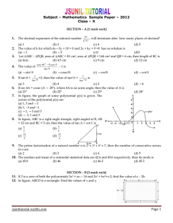y If no unit of angle measure is specified, then radian measure is understood. Figure 2 shows angles measuring 30 radians and 30В°. Be careful not to confuse them. CAUTION x 0 30 radians The following table and Figure 3 on the next page give some equivalent angles measured in degrees and radians. Keep in mind that 180Ш‡ вЂ« вђІ ШЌвЂ¬radians. y Degrees 30В° 0 30 degrees Figure 2 x Radians Degrees Radians Exact Approximate Exact Approximate 0В° 0 0 90В° вђІ 2 1.57 30В° вђІ 6 .52 180В° вђІ 3.14 45В° вђІ 4 .79 270В° 3вђІ 2 4.71 60В° вђІ 3 1.05 360В° 2вђІ 6.28 LIALMC06_0321227638.QXP 2/26/04 10:41 AM Page 536 536 CHAPTER 6 The Circular Functions and Their Graphs 90В° = вђІ 2 60В° = вђІ 120В° = 2вђІ 3 3 45В° = вђІ 135В° = 3вђІ 4 4 30В° = вђІ 150В° = 5вђІ 6 6 Looking Ahead to Calculus In calculus, radian measure is much easier to work with than degree measure. If x is measured in radians, then the derivative of f Н‘xН’ а·‡ sin x is 180В° = вђІ f Р€Н‘xН’ а·‡ cos x. However, if x is measured in degrees, then the derivative of f Н‘xН’ а·‡ sin x is f Р€Н‘xН’ а·‡ 0В° = 0 210В° = 7вђІ 330В° = 11вђІ 6 6 225В° = 5вђІ 315В° = 7вђІ 4 4 240В° = 4вђІ 300В° = 5вђІ 3 270В° = 3вђІ 3 2 вђІ cos x. 180 Figure 3 We use radian measure to simplify certain formulas, two of which follow. Each would be more complicated if expressed in degrees. Arc Length of a Circle We use the first formula to find the length of an arc of a circle. This formula is derived from the fact (proven in geometry) that the length of an arc is proportional to the measure of its central angle. In Figure 4, angle QOP has measure 1 radian and intercepts an arc of length r on the circle. Angle ROT has measure вђЄ radians and intercepts an arc of length s on the circle. Since the lengths of the arcs are proportional to the measures of their central angles, y T Q s R r вђЄ radians 1 radian r O r P x Figure 4 вђЄ s а·‡ . r 1 Multiplying both sides by r gives the following result. Arc Length TEACHING TIP To help students The length s of the arc intercepted on a circle of radius r by a central angle of measure вђЄ radians is given by the product of the radius and the radian measure of the angle, or s вЂ« ШЌвЂ¬rвђЄ, appreciate radian measure, show them that in degrees the formula for arc length is sа·‡ вђЄ вђЄвђІ r Н‘2вђІ rН’ а·‡ . 360 180 (See Exercise 54.) вђЄ in radians. When applying the formula s а·‡ rвђЄ, the value of вђЄ must be expressed in radians. CAUTION LIALMC06_0321227638.QXP 2/26/04 10:41 AM Page 537 6.1 Radian Measure 537 EXAMPLE 3 Finding Arc Length Using s а·‡ rвђЄ A circle has radius 18.2 cm. Find the length of the arc intercepted by a central angle having each of the following measures. (a) 3вђІ radians 8 (b) 144В° Solution (a) As shown in the figure, r а·‡ 18.2 cm and вђЄ а·‡ 38вђІ . s а·‡ rвђЄ s 3вђІ 8 Н©НЄ 3вђІ cm Substitute for r and вђЄ. 8 s а·‡ 18.2 r = 18.2 cm sа·‡ Arc length formula 54.6вђІ cm П· 21.4 cm 8 (b) The formula s а·‡ rвђЄ requires that вђЄ be measured in radians. First, convert вђЄ вђІ to radians by multiplying 144В° by 180 radian. Н© НЄ 144РЉ а·‡ 144 4вђІ вђІ а·‡ radians Convert from degrees to radians. 180 5 The length s is given by Н©НЄ 4вђІ 72.8вђІ П· 45.7 cm. а·‡ 5 5 s а·‡ rвђЄ а·‡ 18.2 Now try Exercises 49 and 51. 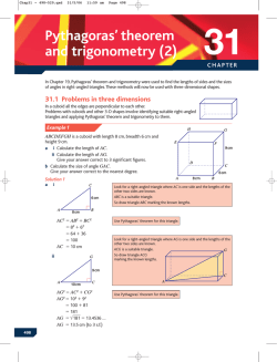EXAMPLE 4 Using Latitudes to Find the Distance Between Two Cities Reno, Nevada, is approximately due north of Los Angeles. The latitude of Reno is 40В° N, while that of Los Angeles is 34В° N. (The N in 34В° N means north of the equator.) The radius of Earth is 6400 km. Find the north-south distance between the two cities. Solution Reno s 6В° Los Angeles Latitude gives the measure of a central angle with vertex at EarthвЂ™s center whose initial side goes through the equator and whose terminal side goes through the given location. As shown in Figure 5, the central angle between Reno and Los Angeles is 40РЉ ПЄ 34РЉ а·‡ 6РЉ. The distance between the two cities can be found by the formula s а·‡ rвђЄ, after 6В° is first converted to radians. Н© НЄ 40В° 34В° 6400 km 6РЉ а·‡ 6 Equator вђІ вђІ а·‡ radian 180 30 The distance between the two cities is Figure 5 Н©НЄ s а·‡ rвђЄ а·‡ 6400 вђІ вђІ П· 670 km. Let r а·‡ 6400 and вђЄ а·‡ 30 . 30 Now try Exercise 55. LIALMC06_0321227638.QXP 2/26/04 10:41 AM Page 538 538 CHAPTER 6 The Circular Functions and Their Graphs EXAMPLE 5 Finding a Length Using s а·‡ rвђЄ 39.72В° A rope is being wound around a drum with radius .8725 ft. (See Figure 6.) How much rope will be wound around the drum if the drum is rotated through an angle of 39.72В°? .8725 ft Solution The length of rope wound around the drum is the arc length for a circle of radius .8725 ft and a central angle of 39.72В°. Use the formula s а·‡ rвђЄ, with the angle converted to radian measure. The length of the rope wound around the drum is approximately Figure 6 Н« Н© НЄН¬ s а·‡ rвђЄ а·‡ .8725 39.72 вђІ 180 П· .6049 ft. Now try Exercise 61(a). 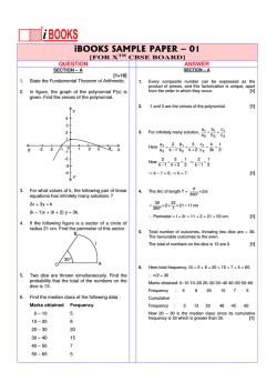EXAMPLE 6 Finding an Angle Measure Using s а·‡ rвђЄ 2. Two gears are adjusted so that the smaller gear drives the larger one, as shown in Figure 7. If the smaller gear rotates through 225В°, through how many degrees will the larger gear rotate? m 5c 4.8 cm Solution First find the radian measure of the angle, and then find the arc length on the smaller gear that determines the motion of the larger gear. Since 5вђІ 225РЉ а·‡ 4 radians, for the smaller gear, Н©НЄ Figure 7 s а·‡ rвђЄ а·‡ 2.5 12.5вђІ 25вђІ 5вђІ а·‡ а·‡ cm. 4 4 8 An arc with this length on the larger gear corresponds to an angle measure вђЄ, in radians, where s а·‡ rвђЄ 25вђІ а·‡ 4.8вђЄ 8 125вђІ П· вђЄ. 192 Substitute 258вђІ for s and 4.8 for r. 48 24 4.8 а·‡ 10 а·‡ 5 ; multiply 5 by 24 to solve for вђЄ. Converting вђЄ back to degrees shows that the larger gear rotates through Н© НЄ 125вђІ 180РЉ вђІ П· 117РЉ. Convert вђЄ а·‡ 125 192 to degrees. 192 вђІ Now try Exercise 63. вђЄ r Figure 8 The shaded region is a sector of the circle. Area of a Sector of a Circle A sector of a circle is the portion of the interior of a circle intercepted by a central angle. Think of it as a вЂњpiece of pie.вЂќ See Figure 8. A complete circle can be thought of as an angle with measure 2вђІ radians. If a central angle for a sector has measure вђЄ radians, then the sector вђЄ makes up the fraction 2вђІ of a complete circle. The area of a complete circle with 2 radius r is A а·‡ вђІr . Therefore, area of the sector а·‡ 1 вђЄ Н‘вђІ r 2Н’ а·‡ r 2вђЄ, 2вђІ 2 вђЄ in radians. LIALMC06_0321227638.QXP 2/26/04 10:41 AM Page 539 6.1 Radian Measure 539 This discussion is summarized as follows. Area of a Sector The area of a sector of a circle of radius r and central angle вђЄ is given by AвЂ«ШЌвЂ¬ 1 2 r вђЄ, 2 вђЄ in radians. As in the formula for arc length, the value of вђЄ must be in radians when using this formula for the area of a sector. CAUTION EXAMPLE 7 Finding the Area of a Sector-Shaped Field 321 m Find the area of the sector-shaped field shown in Figure 9. 15В° Solution First, convert 15В° to radians. Н© НЄ 15РЉ а·‡ 15 вђІ вђІ а·‡ radian 180 12 Now use the formula to find the area of a sector of a circle with radius r а·‡ 321. Aа·‡ Figure 9 Н©НЄ 1 2 1 вђІ r вђЄ а·‡ Н‘321Н’2 П· 13,500 m2 2 2 12 Now try Exercise 77. 6.1 Exercises вђІ вђІ 5вђІ 3вђІ 2. 3. 4. 3 2 6 2 7вђІ 8вђІ вђІ 5. 6. 7. ПЄ 4 3 4 7вђІ 8. ПЄ 9. .68 10. 1.29 6 11. 2.43 12. 3.05 13. 1.122 14. 2.140 15. 1 16. 2 1. Convert each degree measure to radians. Leave answers as multiples of вђІ. See Example 1(a). 1. 60РЉ 2. 90РЉ 3. 150РЉ 4. 270РЉ 5. 315РЉ 6. 480РЉ 7. ПЄ45РЉ 8. ПЄ210РЉ Convert each degree measure to radians. See Example 1(b). 9. 39РЉ 12. 174РЉ 50Р€ 10. 74РЉ 11. 139РЉ 10Р€ 13. 64.29РЉ 14. 122.62РЉ Concept Check In Exercises 15 вЂ“18, each angle вђЄ is an integer when measured in radians. Give the radian measure of the angle. 15. Оё 0 y 16. y Оё x 0 x LIALMC06_0321227638.QXP 2/26/04 10:41 AM Page 540 540 CHAPTER 6 The Circular Functions and Their Graphs 3 18. ПЄ1 21. 60РЉ 480РЉ 23. 315РЉ 24. 120РЉ 330РЉ 26. 675РЉ 27. ПЄ30РЉ ПЄ63РЉ 29. 114.6РЉ 286.5РЉ 31. 99.7РЉ 32. 19.6РЉ ПЄ564.2РЉ 34. ПЄ198.9РЉ Н™3 35. 1 36. Н™2 37. ПЄ 3 1 1 38. 39. ПЄ1 40. 2 2 Н™3 41. 42. ПЄ1 2 17. 22. 25. 28. 30. 33. y 17. 18. y Оё x 0 9 19. x Оё 0 In your own words, explain how to convert (a) degree measure to radian measure; (b) radian measure to degree measure. 9 20. Explain the difference between degree measure and radian measure. Convert each radian measure to degrees. See Example 2(a). вђІ 3 11вђІ 25. 6 21. 22. 8вђІ 3 23. 7вђІ 4 26. 15вђІ 4 27. ПЄ 24. вђІ 6 2вђІ 3 28. ПЄ 7вђІ 20 Convert each radian measure to degrees. Give answers using decimal degrees to the nearest tenth. See Example 2(b). 29. 2 30. 5 31. 1.74 32. .3417 33. ПЄ9.84763 34. ПЄ3.47189 Relating Concepts For individual or collaborative investigation (Exercises 35вЂ“42) In anticipation of the material in the next section, we show how to find the trigonometric function values of radian-measured angles. Suppose we want to find sin 56вђІ . One way to do this is to convert 56вђІ radians to 150В°, and then use the methods of Chapter 5 to evaluate: sin 1 5вђІ а·‡ sin 150РЉ а·‡ П© sin 30РЉ а·‡ . (Section 5.3) 6 2 Sine is positive in quadrant II. Reference angle for 150РЉ Use this technique to find each function value. Give exact values. 35. tan вђІ 4 39. sec вђІ 36. csc вђІ 4 Н© НЄ 40. sin ПЄ 7вђІ 6 37. cot 2вђІ 3 Н© НЄ 41. cos ПЄ вђІ 6 38. cos вђІ 3 Н© НЄ 42. tan ПЄ 9вђІ 4 LIALMC06_0321227638.QXP 2/26/04 10:41 AM Page 541 6.1 Radian Measure 541 2вђІ 44. 4вђІ 45. 8 46. 6 1 48. 1.5 49. 25.8 cm 3.08 cm 51. 5.05 m 169 cm 53. The length is вђІrвђЄ doubled. 54. s а·‡ 180 55. 3500 km 56. 1500 km 57. 5900 km 58. 8800 km 43. 47. 50. 52. Concept Check angle. Find the exact length of each arc intercepted by the given central 43. 44. вђІ 3 12 вђІ 2 4 Concept Check 45. Find the radius of each circle. 46. 6вђІ вђІ 2 3вђІ 4 Concept Check 3вђІ Find the measure of each central angle (in radians). 47. 48. 3 6 вђЄ вђЄ 3 4 Unless otherwise directed, give calculator approximations in your answers in the rest of this exercise set. Find the length of each arc intercepted by a central angle вђЄ in a circle of radius r. See Example 3. 49. r а·‡ 12.3 cm, вђЄ а·‡ 2вђІ radians 3 51. r а·‡ 4.82 m, вђЄ а·‡ 60РЉ 50. r а·‡ .892 cm, вђЄ а·‡ 11вђІ radians 10 52. r а·‡ 71.9 cm, вђЄ а·‡ 135РЉ 53. Concept Check If the radius of a circle is doubled, how is the length of the arc intercepted by a fixed central angle changed? 54. Concept Check Radian measure simplifies many formulas, such as the formula for arc length, s а·‡ r вђЄ. Give the corresponding formula when вђЄ is measured in degrees instead of radians. Distance Between Cities Find the distance in kilometers between each pair of cities, assuming they lie on the same north-south line. See Example 4. 55. Panama City, Panama, 9РЉ N, and Pittsburgh, Pennsylvania, 40РЉ N 56. Farmersville, California, 36РЉ N, and Penticton, British Columbia, 49РЉ N 57. New York City, New York, 41РЉ N, and Lima, Peru, 12РЉ S 58. Halifax, Nova Scotia, 45РЉ N, and Buenos Aires, Argentina, 34РЉ S LIALMC06_0321227638.QXP 2/26/04 10:41 AM Page 542 542 CHAPTER 6 The Circular Functions and Their Graphs 59. 61. 62. 64. 66. 44РЉ N 60. 43РЉ N (a) 11.6 in. (b) 37РЉ 5Р€ 12.7 cm 63. 38.5РЉ 18.7 cm 65. 146 in. (a) 39,616 rotations 59. Latitude of Madison Madison, South Dakota, and Dallas, Texas, are 1200 km apart and lie on the same north-south line. The latitude of Dallas is 33РЉ N. What is the latitude of Madison? 60. Latitude of Toronto Charleston, South Carolina, and Toronto, Canada, are 1100 km apart and lie on the same north-south line. The latitude of Charleston is 33РЉ N. What is the latitude of Toronto? Work each problem. See Examples 5 and 6. 61. Pulley Raising a Weight (a) How many inches will the weight in the figure rise if the pulley is rotated through an angle of 71РЉ 50Р€? (b) Through what angle, to the nearest minute, must the pulley be rotated to raise the weight 6 in.? 9.27 in. 62. Pulley Raising a Weight Find the radius of the pulley in the figure if a rotation of 51.6РЉ raises the weight 11.4 cm. r 63. Rotating Wheels The rotation of the smaller wheel in the figure causes the larger wheel to rotate. Through how many degrees will the larger wheel rotate if the smaller one rotates through 60.0РЉ? 64. Rotating Wheels Find the radius of the larger wheel in the figure if the smaller wheel rotates 80.0РЉ when the larger wheel rotates 50.0РЉ. 65. Bicycle Chain Drive The figure shows the chain drive of a bicycle. How far will the bicycle move if the pedals are rotated through 180РЉ? Assume the radius of the bicycle wheel is 13.6 in. 8 .1 6 cm 5.23 cm 11.7 cm r 1.38 in. 4.72 in. 66. Pickup Truck Speedometer The speedometer of TerryвЂ™s small pickup truck is designed to be accurate with tires of radius 14 in. (a) Find the number of rotations of a tire in 1 hr if the truck is driven at 55 mph. LIALMC06_0321227638.QXP 2/26/04 10:41 AM Page 543 6.1 Radian Measure 543 66. 67. 69. 72. 74. 76. 78. 80. 82. (b) 62.9 mi; yes .20 km 68. 850 ft 6вђІ 70. 16вђІ 71. 1.5 1 73. 1116.1 m2 3744.8 km2 75. 706.9 ft 2 10,602.9 yd2 77. 114.0 cm2 365.3 m2 79. 1885.0 mi2 19,085.2 km2 81. 3.6 16 m (b) Suppose that oversize tires of radius 16 in. are placed on the truck. If the truck is now driven for 1 hr with the speedometer reading 55 mph, how far has the truck gone? If the speed limit is 55 mph, does Terry deserve a speeding ticket? If a central angle is very small, there is little difference in length between an arc and the inscribed chord. See the figure. Approximate each of the following lengths by finding the necessary arc length. (Note: When a central angle intercepts an arc, the arc is said to subtend the angle.) Arc length в‰€ length of inscribed chord Arc Inscribed chord 67. Length of a Train A railroad track in the desert is 3.5 km away. A train on the track subtends (horizontally) an angle of 3РЉ 20Р€. Find the length of the train. 68. Distance to a Boat The mast of Brent SimonвЂ™s boat is 32 ft high. If it subtends an angle of 2РЉ 10Р€, how far away is it? Concept Check Find the area of each sector. 69. 70. 4вђІ 2вђІ вђЄ вђЄ 6 8 Concept Check Find the measure (in radians) of each central angle. The number inside the sector is the area. 71. 72. 3 sq units 8 sq units 2 4 Find the area of a sector of a circle having radius r and central angle вђЄ. See Example 7. 73. r а·‡ 29.2 m, вђЄ а·‡ 5вђІ radians 6 вђІ radians 2 77. r а·‡ 12.7 cm, вђЄ а·‡ 81РЉ 79. r а·‡ 40.0 mi, вђЄ а·‡ 135РЉ 75. r а·‡ 30.0 ft, вђЄ а·‡ 74. r а·‡ 59.8 km, вђЄ а·‡ 2вђІ radians 3 76. r а·‡ 90.0 yd, вђЄ а·‡ 5вђІ radians 6 78. r а·‡ 18.3 m, вђЄ а·‡ 125РЉ 80. r а·‡ 90.0 km, вђЄ а·‡ 270РЉ Work each problem. 81. Find the measure (in radians) of a central angle of a sector of area 16 in.2 in a circle of radius 3.0 in. 82. Find the radius of a circle in which a central angle of вђІ6 radian determines a sector of area 64 m2. LIALMC06_0321227638.QXP 2/26/04 10:41 AM Page 544 544 CHAPTER 6 The Circular Functions and Their Graphs 83. (a) 13 1 2вђІ (b) 480 ft РЉ; 3 27 160 П· 17.8 ft 9 (d) approximately 672 ft 2 84. 75.4 in.2 85. (a) 140 ft (b) 102 ft (c) 622 ft 2 86. (a) 550 m (b) 1800 m 87. 1900 yd2 88. 1.15 mi 83. Measures of a Structure The figure shows Medicine Wheel, a Native American structure in northern Wyoming. This circular structure is perhaps 2500 yr old. There are 27 aboriginal spokes in the wheel, all equally spaced. (c) Find the measure of each central angle in degrees and in radians. If the radius of the wheel is 76 ft, find the circumference. Find the length of each arc intercepted by consecutive pairs of spokes. Find the area of each sector formed by consecutive spokes. 95В° 7i n. in . 84. Area Cleaned by a Windshield Wiper The Ford Model A, built from 1928 to 1931, had a single windshield wiper on the driverвЂ™s side. The total arm and blade was 10 in. long and rotated back and forth through an angle of 95РЉ. The shaded region in the figure is the portion of the windshield cleaned by the 7-in. wiper blade. What is the area of the region cleaned? 10 (a) (b) (c) (d) 85. Circular Railroad Curves In the United States, circular railroad curves are designated by the degree of curvature, the central angle subtended by a chord of 100 ft. Suppose a portion of track has curvature 42РЉ. (Source: Hay, W., Railroad Engineering, John Wiley & Sons, 1982.) (a) What is the radius of the curve? (b) What is the length of the arc determined by the 100-ft chord? (c) What is the area of the portion of the circle bounded by the arc and the 100-ft chord? 86. Land Required for a Solar-Power Plant A 300-megawatt solar-power plant requires approximately 950,000 m2 of land area in order to collect the required amount of energy from sunlight. (a) If this land area is circular, what is its radius? (b) If this land area is a 35РЉ sector of a circle, what is its radius? 87. Area of a Lot A frequent problem in surveying city lots and rural lands adjacent to curves of highways and railways is that of finding the area when one or more of the boundary lines is the arc of a circle. Find the area of the lot shown in the figure. (Source: Anderson, J. and E. Michael, Introduction to Surveying, McGraw-Hill, 1985.) 88. Nautical Miles Nautical miles are used by ships and airplanes. They are different from statute miles, which equal 5280 ft. A nautical mile is defined to be the arc length along the equator intercepted by a central angle AOB of 1 min, as illustrated in the figure. If the equatorial radius of Earth is 3963 mi, use the arc length formula to approximate the number of statute miles in 1 nautical mile. Round your answer to two decimal places. 40 yd 60В° 30 yd O B A Nautical mile Not to scale LIALMC06_0321227638.QXP 2/26/04 10:41 AM Page 545 6.2 The Unit Circle and Circular Functions 545 89. radius: 3947 mi; circumference: 24,800 mi 90. approximately 2156 mi 91. The area is quadrupled. вђІ r 2вђЄ 92. A а·‡ 360 89. Circumference of Earth The first accurate estimate of the distance around Earth was done by the Greek astronomer Eratosthenes (276 вЂ“195 B.C.), who noted that the noontime position of the sun at the summer solstice differed by 7РЉ 12Р€ from the city of Syene to the city of Alexandria. (See the figure.) The distance between these two cities is 496 mi. Use the arc length formula to estimate the radius of Earth. Then find the circumference of Earth. (Source: Zeilik, M., Introductory Astronomy and Astrophysics, Third Edition, Saunders College Publishers, 1992.) Sun's rays at noon 496 mi 7В° 12' Shadow Syene Alexandria 7В° 12' 90. Diameter of the Moon The distance to the moon is approximately 238,900 mi. Use the arc length formula to estimate the diameter d of the moon if angle вђЄ in the figure is measured to be .517РЉ. вђЄ d Not to scale 91. Concept Check If the radius of a circle is doubled and the central angle of a sector is unchanged, how is the area of the sector changed? 92. Concept Check Give the corresponding formula for the area of a sector when the angle is measured in degrees. 6.2 The Unit Circle and Circular Functions Circular Functions в– Finding Values of Circular Functions Function Value в– Angular and Linear Speed x = cos s y = sin s Arc of length s (0, 1) (x, y) вђЄ (1, 0) 0 (0, вЂ“1) Unit circle x2 + y2 = 1 Figure 10 Determining a Number with a Given Circular In Section 5.2, we defined the six trigonometric functions in such a way that the domain of each function was a set of angles in standard position. These angles can be measured in degrees or in radians. In advanced courses, such as calculus, it is necessary to modify the trigonometric functions so that their domains consist of real numbers rather than angles. We do this by using the relationship between an angle вђЄ and an arc of length s on a circle. y (вЂ“1, 0) в– x Circular Functions In Figure 10, we start at the point Н‘1, 0Н’ and measure an arc of length s along the circle. If s Пѕ 0, then the arc is measured in a counterclockwise direction, and if s ПЅ 0, then the direction is clockwise. (If s а·‡ 0, then no arc is measured.) Let the endpoint of this arc be at the point Н‘x, yН’. The circle in Figure 10 is a unit circleвЂ” it has center at the origin and radius 1 unit (hence the name unit circle). Recall from algebra that the equation of this circle is x 2 П© y 2 а·‡ 1. (Section 2.1) LIALMC06_0321227638.QXP 2/26/04 10:41 AM Page 546 546 CHAPTER 6 The Circular Functions and Their Graphs We saw in the previous section that the radian measure of вђЄ is related to the arc length s. In fact, for вђЄ measured in radians, we know that s а·‡ rвђЄ. Here, r а·‡ 1, so s, which is measured in linear units such as inches or centimeters, is numerically equal to вђЄ, measured in radians. Thus, the trigonometric functions of angle вђЄ in radians found by choosing a point Н‘x, yН’ on the unit circle can be rewritten as functions of the arc length s, a real number. When interpreted this way, they are called circular functions. Looking Ahead to Calculus Circular Functions If you plan to study calculus, you must become very familiar with radian measure. In calculus, the trigonometric or circular functions are always understood to have real number domains. sin s вЂ« ШЌвЂ¬y csc s вЂ«ШЌвЂ¬ 1 y cos s вЂ« ШЌвЂ¬x (y sec s вЂ«ШЌвЂ¬ 0) 1 x (x 0) tan s вЂ«ШЌвЂ¬ y x (x 0) cot s вЂ«ШЌвЂ¬ x y (y 0) Since x represents the cosine of s and y represents the sine of s, and because of the discussion in Section 6.1 on converting between degrees and radians, we can summarize a great deal of information in a concise manner, as seen in Figure 11.* y (вЂ“ 12 , в€љ32 ) вђІ (0, 1) ( 12 , в€љ32 ) 90В° вђІ (вЂ“ в€љ22 , в€љ22 ) 3вђІ 2вђІ3 120В°2 60В° 3 вђІ ( в€љ22 , в€љ22 ) 45В° 4 в€љ3 , 1 вђІ (вЂ“ в€љ32 , 12 ) 5вђІ 4 135В° 30В° 6 ( 2 2 ) TEACHING TIP Draw a unit circle on the chalkboard and trace a point slowly counterclockwise, starting at Н‘1, 0Н’. Students should see that the y-value (sine function) starts at 0, increases to 1 (at вђІ2 radians), decreases to 0 (at вђІ radians), decreases again to ПЄ1 (at 32вђІ radians), and returns to 0 after one full revolution (2вђІ radians). This type of analysis will help illustrate the range associated with the sine and cosine functions. ( 6 150В° (вЂ“1, 0) 180В° вђІ 7вђІ 210В° 6 вЂ“ в€љ3 , вЂ“ 1 5вђІ 225В° 2 ( вЂ“ в€љ2 , 2 2 ) вЂ“ в€љ2 2 ( 4 ) вЂ“ 1, 2 4вђІ 3 вЂ“ в€љ3 2 ) 0 0В° 0 (1, 0) x 360В° 2вђІ 330В° 11вђІ в€љ3 , 1 6 вЂ“ 315В° 7вђІ (2 240В° 300В° 5вђІ 4 в€љ2 , вЂ“ в€љ2 3 3вђІ 2 2 270В° 2 1 , в€љ3 (0, вЂ“1) 2 вЂ“ 2 ( ( 2 ) ) ) Unit circle x2 + y2 = 1 Figure 11 Since sin s а·‡ y and cos s а·‡ x, we can replace x and y in the equation x 2 П© y 2 а·‡ 1 and obtain the Pythagorean identity NOTE cos2 s П© sin2 s а·‡ 1. The ordered pair Н‘x, yН’ represents a point on the unit circle, and therefore so ПЄ1 Х… x Х… 1 and ПЄ1 Х… y Х… 1, ПЄ1 Х… cos s Х… 1 and ПЄ1 Х… sin s Х… 1. *The authors thank Professor Marvel Townsend of the University of Florida for her suggestion to include this figure. LIALMC06_0321227638.QXP 2/26/04 10:41 AM Page 547 6.2 The Unit Circle and Circular Functions 547 For any value of s, both sin s and cos s exist, so the domain of these functions is y the set of all real numbers. For tan s, defined as x , x must not equal 0. The only вђІ вђІ 3вђІ 3вђІ way x can equal 0 is when the arc length s is 2 , ПЄ 2 , 2 , ПЄ 2 , and so on. To avoid a 0 denominator, the domain of the tangent function must be restricted to those values of s satisfying s Н‘2n П© 1Н’ вђІ , 2 n any integer. The definition of secant also has x in the denominator, so the domain of secant is the same as the domain of tangent. Both cotangent and cosecant are defined with a denominator of y. To guarantee that y 0, the domain of these functions must be the set of all values of s satisfying s nвђІ , n any integer. In summary, the domains of the circular functions are as follows. Domains of the Circular Functions Assume that n is any integer and s is a real number. Sine and Cosine Functions: (ШЉШ•, Ш•) Tangent and Secant Functions: Н sН‰ s Cotangent and Cosecant Functions: (cos s, sin s) = (x, y) y (0, 1) вђЄ (вЂ“1, 0) s=вђЄ x 0 (1, 0) x =1 {s Н‰ s nвђІ} вђІ 2 Н® Finding Values of Circular Functions The circular functions (functions of real numbers) are closely related to the trigonometric functions of angles measured in radians. To see this, let us assume that angle вђЄ is in standard position, superimposed on the unit circle, as shown in Figure 12. Suppose further that вђЄ is the radian measure of this angle. Using the arc length formula s а·‡ rвђЄ with r а·‡ 1, we have s а·‡ вђЄ. Thus, the length of the intercepted arc is the real number that corresponds to the radian measure of вђЄ. Using the definitions of the trigonometric functions, we have (0, вЂ“1) 2 + y2 (2n Ш‰ 1) sin вђЄ а·‡ y y а·‡ а·‡ y а·‡ sin s, r 1 and cos вђЄ а·‡ x x а·‡ а·‡ x а·‡ cos s, r 1 Figure 12 and so on. As shown here, the trigonometric functions and the circular functions lead to the same function values, provided we think of the angles as being in radian measure. This leads to the following important result concerning evaluation of circular functions. Evaluating a Circular Function Circular function values of real numbers are obtained in the same manner as trigonometric function values of angles measured in radians. This applies both to methods of finding exact values (such as reference angle analysis) and to calculator approximations. Calculators must be in radian mode when finding circular function values. LIALMC06_0321227638.QXP 2/26/04 10:41 AM Page 548 548 CHAPTER 6 The Circular Functions and Their Graphs EXAMPLE 1 Finding Exact Circular Function Values Find the exact values of sin 32вђІ , cos 32вђІ , and tan 32вђІ . Evaluating a circular function at the real number 32вђІ is equivalent to evaluating it at 32вђІ radians. An angle of 32вђІ radians intersects the unit circle at the point Н‘0, ПЄ1Н’, as shown in Figure 13. Since y Solution (0, 1) (вЂ“1, 0) вђЄ = 3вђІ 2 0 sin s а·‡ y, x cos s а·‡ x, tan s а·‡ and (1, 0) y , x it follows that (0, вЂ“1) sin 3вђІ а·‡ ПЄ1, 2 cos 3вђІ а·‡ 0, 2 and tan 3вђІ is undefined. 2 Figure 13 Now try Exercise 1. EXAMPLE 2 Finding Exact Circular Function Values TEACHING TIP Point out the importance of being able to sketch the unit circle as in Figure 13. This will enable students to more easily determine function values of mulвђІ . tiples of 2 (a) Use Figure 11 to find the exact values of cos 74вђІ and sin 74вђІ . (b) Use Figure 11 to find the exact value of tanН‘ ПЄ 53вђІ Н’. (c) Use reference angles and degree/radian conversion to find the exact value of cos 23вђІ . Solution (a) In Figure 11, we see that the terminal side of Н™2 Н™2 circle at Н‘ 2 ,ПЄ 2 Н’. Thus, cos 7вђІ Н™2 а·‡ 4 2 (b) Angles of ПЄ 53вђІ radians and intersect the unit circle at Н‘ and sin вђІ 3 radians 1 Н™3 2 , 2 , so Н© НЄ 7вђІ 4 radians intersects the unit 7вђІ Н™2 а·‡ПЄ . 4 2 are coterminal. Their terminal sides Н’ 5вђІ вђІ tan ПЄ а·‡ tan а·‡ 3 3 Н™3 2 1 2 а·‡ Н™3. (c) An angle of 23вђІ radians corresponds to an angle of 120В°. In standard position, 120В° lies in quadrant II with a reference angle of 60В°, so Cosine is negative in quadrant II. cos 2вђІ 1 а·‡ cos 120В° а·‡ ПЄcos 60РЉ а·‡ ПЄ . 3 2 Reference angle (Section 5.3) Now try Exercises 7, 17, and 21. Examples 1 and 2 illustrate that there are several methods of finding exact circular function values. NOTE LIALMC06_0321227638.QXP 2/26/04 10:41 AM Page 549 6.2 The Unit Circle and Circular Functions 549 EXAMPLE 3 Approximating Circular Function Values Find a calculator approximation to four decimal places for each circular function value. (a) cos 1.85 (b) cos .5149 (c) cot 1.3209 ( d ) secН‘ПЄ2.9234Н’ Solution (a) With a calculator in radian mode, we find cos 1.85 П· ПЄ.2756. (b) cos .5149 П· .8703 Use a calculator in radian mode. Radian mode This is how a calculator displays the result of Example 3(a), correct to four decimal digits. TEACHING TIP Remind students ПЄ1 ПЄ1 not to use the sin , cos , and tanПЄ1, keys when evaluating reciprocal functions with a calculator. (c) As before, to find cotangent, secant, and cosecant function values, we must use the appropriate reciprocal functions. To find cot 1.3209, first find tan 1.3209 and then find the reciprocal. cot 1.3209 а·‡ (d) secН‘ПЄ2.9234Н’ а·‡ 1 П· .2552 tan 1.3209 1 П· ПЄ1.0243 cosН‘ПЄ2.9234Н’ Now try Exercises 23, 29, and 33. CAUTION A common error in trigonometry is using calculators in degree mode when radian mode should be used. Remember, if you are finding a circular function value of a real number, the calculator must be in radian mode. Determining a Number with a Given Circular Function Value Recall from Section 5.3 how we used a calculator to determine an angle measure, given a trigonometric function value of the angle. EXAMPLE 4 Finding a Number Given Its Circular Function Value (a) Approximate the value of s in the interval Н“ 0, вђІ2 Н”, if cos s а·‡ .9685. (b) Find the exact value of s in the interval Н“ вђІ, 32вђІ Н”, if tan s а·‡ 1. The calculator is set to show four decimal digits in the answer. Figure 14 Solution (a) Since we are given a cosine value and want to determine the real number in Н“ 0, вђІ2 Н” having this cosine value, we use the inverse cosine function of a calculator. With the calculator in radian mode, we find cosПЄ1Н‘.9685Н’ П· .2517. (Section 5.3) See Figure 14. (Refer to your ownerвЂ™s manual to determine how to evaluate the sinПЄ1, cosПЄ1, and tanПЄ1 functions with your calculator.) (b) Recall that tan вђІ4 а·‡ 1, and in quadrant III tan s is positive. Therefore, This screen supports the result of Example 4(b). The calculator is in radian mode. Figure 15 Н© tan вђІ П© вђІ 4 НЄ а·‡ tan 5вђІ а·‡ 1, 4 and s а·‡ 54вђІ . Figure 15 supports this result. Now try Exercises 49 and 55. LIALMC06_0321227638.QXP 2/26/04 10:41 AM Page 550 550 CHAPTER 6 The Circular Functions and Their Graphs CONNECTIONS A convenient way to see the sine, cosine, and tangent trigonometric ratios geometrically is shown in Figure 16 for вђЄ in quadrants I and II. The circle shown is the unit circle, which has radius 1. By remembering this figure and the segments that represent the sine, cosine, and tangent functions, you can quickly recall properties of the trigonometric functions. Horizontal line segments to the left of the origin and vertical line segments below the x-axis represent negative values. Note that the tangent line must be tangent to the circle at Н‘1, 0Н’, for any quadrant in which вђЄ lies. y y sin вђЄ tan вђЄ 1 вђЄ cos вђЄ sin вђЄ 1 вђЄ (1, 0) x x cos вђЄ (1, 0) tan вђЄ вђЄ in quadrant II вђЄ in quadrant I Figure 16 y PQ а·‡ y а·‡ а·‡ sin вђЄ ; 1 x OQ а·‡ x а·‡ а·‡ cos вђЄ ; 1 y AB AB а·‡ а·‡ AB а·‡ 1 AO x (by similar triangles) а·‡ tan вђЄ For Discussion or Writing See Figure 17. Use the definition of the trigonometric functions and similar triangles to show that PQ а·‡ sin вђЄ, OQ а·‡ cos вђЄ, and AB а·‡ tan вђЄ. B P(x, y) 1 вђЄ O y x A(1, 0) Q Figure 17 Angular and Linear Speed The human joint that can be flexed the fastest вђІ is the wrist, which can rotate through 90В°, or 2 radians, in .045 sec while holding a tennis racket. Angular speed вђ» (omega) measures the speed of rotation and is defined by вђЄ вђ»а·‡ , t where вђЄ is the angle of rotation in radians and t is time. The angular speed of a human wrist swinging a tennis racket is вђ»а·‡ вђІ вђЄ а·‡ 2 П· 35 radians per sec. t .045 The linear speed v at which the tip of the racket travels as a result of flexing the wrist is given by v а·‡ rвђ», where r is the radius (distance) from the tip of the racket to the wrist joint. If r а·‡ 2 ft, then the speed at the tip of the racket is v а·‡ rвђ» П· 2Н‘35Н’ а·‡ 70 ft per sec, or about 48 mph. LIALMC06_0321227638.QXP 2/26/04 10:41 AM Page 551 6.2 The Unit Circle and Circular Functions 551 In a tennis serve the arm rotates at the shoulder, so the final speed of the racket is considerably faster. (Source: Cooper, J. and R. Glassow, Kinesiology, Second Edition, C.V. Mosby, 1968.) EXAMPLE 5 Finding Angular Speed of a Pulley and Linear Speed of a Belt A belt runs a pulley of radius 6 cm at 80 revolutions per min. (a) Find the angular speed of the pulley in radians per second. (b) Find the linear speed of the belt in centimeters per second. Solution TEACHING TIP Mention that, while problems involving linear and angular speed can be solved using the formula for circumference, the formulas presented in this section are much more efficient. (a) In 1 min, the pulley makes 80 revolutions. Each revolution is 2вђІ radians, for a total of 80Н‘2вђІН’ а·‡ 160вђІ radians per min. Since there are 60 sec in 1 min, we find вђ», the angular speed in radians per second, by dividing 160вђІ by 60. вђ»а·‡ 160вђІ 8вђІ а·‡ radians per sec 60 3 (b) The linear speed of the belt will be the same as that of a point on the circumference of the pulley. Thus, Н©НЄ v а·‡ rвђ» а·‡ 6 8вђІ а·‡ 16вђІ П· 50.3 cm per sec. 3 Now try Exercise 95. Suppose that an object is moving at a constant speed. If it travels a distance s in time t, then its linear speed v is given by vа·‡ s . t If the object is traveling in a circle, then s а·‡ rвђЄ, where r is the radius of the circle and вђЄ is the angle of rotation. Thus, we can write vа·‡ rвђЄ . t The formulas for angular and linear speed are summarized in the table. Angular Speed вђ»вЂ«ШЌвЂ¬ вђЄ t (вђ» in radians per unit time, вђЄ in radians) Linear Speed vвЂ«ШЌвЂ¬ s t vвЂ«ШЌвЂ¬ rвђЄ t v вЂ« ШЌвЂ¬rвђ» LIALMC06_0321227638.QXP 2/26/04 10:41 AM Page 552 552 CHAPTER 6 The Circular Functions and Their Graphs EXAMPLE 6 Finding Linear Speed and Distance Traveled by a Satellite 1600 km Satellite 6400 km A satellite traveling in a circular orbit 1600 km above the surface of Earth takes 2 hr to make an orbit. The radius of Earth is 6400 km. See Figure 18. (a) Find the linear speed of the satellite. (b) Find the distance the satellite travels in 4.5 hr. Solution Earth (a) The distance of the satellite from the center of Earth is r а·‡ 1600 П© 6400 а·‡ 8000 km. Not to scale Figure 18 For one orbit, вђЄ а·‡ 2вђІ, and s а·‡ rвђЄ а·‡ 8000Н‘2вђІН’ km. (Section 6.1) Since it takes 2 hr to complete an orbit, the linear speed is vа·‡ 8000Н‘2вђІН’ s а·‡ а·‡ 8000вђІ П· 25,000 km per hr. t 2 (b) s а·‡ vt а·‡ 8000вђІ Н‘4.5Н’ а·‡ 36,000вђІ П· 110,000 km Now try Exercise 93. 6.2 Exercises 1. 2. 3. 4. 5. 6. (a) 1 (a) 0 (a) 0 (a) 0 (a) 0 (a) 1 1 7. ПЄ 2 11. 14. 17. 20. 23. 26. 28. 30. 32. 34. (b) 0 (c) undefined (b) ПЄ1 (c) 0 (b) 1 (c) 0 (b) ПЄ1 (c) 0 (b) ПЄ1 (c) 0 (b) 0 (c) undefined 1 8. 9. ПЄ1 10. ПЄ2 2 1 ПЄ2 12. ПЄН™3 13. ПЄ 2 Н™2 16. ПЄН™2 ПЄН™3 15. 2 1 2Н™3 Н™3 18. ПЄ 19. 2 2 3 2Н™3 Н™2 Н™3 21. ПЄ 22. ПЄ 3 3 2 .5736 24. .7314 25. .4068 .5397 27. 1.2065 .1944 29. 14.3338 1.0170 31. ПЄ1.0460 ПЄ2.1291 33. ПЄ3.8665 1.1848 For each value of вђЄ, find (a) sin вђЄ, (b) cos вђЄ, and (c) tan вђЄ. See Example 1. 1. вђЄ а·‡ вђІ 2 4. вђЄ а·‡ 3вђІ 2. вђЄ а·‡ вђІ 3. вђЄ а·‡ 2вђІ 5. вђЄ а·‡ ПЄвђІ 6. вђЄ а·‡ ПЄ 3вђІ 2 Find the exact circular function value for each of the following. See Example 2. 7. sin 7вђІ 6 8. cos 5вђІ 3 9. tan 3вђІ 4 10. sec 2вђІ 3 4вђІ 3 14. tan 17вђІ 3 4вђІ 3 18. sin ПЄ Н© НЄ Н© НЄ 11. csc 11вђІ 6 12. cot 5вђІ 6 13. cos ПЄ 15. cos 7вђІ 4 16. sec 5вђІ 4 17. sin ПЄ 19. sec 23вђІ 6 20. csc 13вђІ 3 21. tan 5вђІ 6 Н© НЄ 22. cos 5вђІ 6 3вђІ 4 Find a calculator approximation for each circular function value. See Example 3. 23. sin .6109 24. sin .8203 25. cosН‘ПЄ1.1519Н’ 26. cosН‘ПЄ5.2825Н’ 27. tan 4.0203 28. tan 6.4752 29. cscН‘ПЄ9.4946Н’ 30. csc 1.3875 31. sec 2.8440 32. secН‘ПЄ8.3429Н’ 33. cot 6.0301 34. cot 3.8426 LIALMC06_0321227638.QXP 2/26/04 10:41 AM Page 553 6.2 The Unit Circle and Circular Functions 553 .7 36. ПЄ.75 37. 4 4.4 39. negative negative 41. negative positive 43. positive negative Н™2 Н™2 45. sin вђЄ а·‡ ; cos вђЄ а·‡ ; 2 2 tan вђЄ а·‡ 1; cot вђЄ а·‡ 1; sec вђЄ а·‡ Н™2; csc вђЄ а·‡ Н™2 8 15 46. sin вђЄ а·‡ ; cos вђЄ а·‡ ПЄ ; 17 17 8 15 tan вђЄ а·‡ ПЄ ; cot вђЄ а·‡ ПЄ ; 15 8 17 17 sec вђЄ а·‡ ПЄ ; csc вђЄ а·‡ 15 8 12 5 47. sin вђЄ а·‡ ПЄ ; cos вђЄ а·‡ ; 13 13 12 5 tan вђЄ а·‡ ПЄ ; cot вђЄ а·‡ ПЄ ; 5 12 13 13 sec вђЄ а·‡ ; csc вђЄ а·‡ ПЄ 5 12 1 Н™3 48. sin вђЄ а·‡ ПЄ ; cos вђЄ а·‡ ПЄ ; 2 2 Н™3 ; cot вђЄ а·‡ Н™3; tan вђЄ а·‡ 3 2Н™3 ; csc вђЄ а·‡ ПЄ2 sec вђЄ а·‡ ПЄ 3 49. .2095 50. .6720 51. 1.4426 52. 1.2799 53. .3887 54. 1.3634 2вђІ 5вђІ 55. 56. 6 3 35. 38. 40. 42. 44. Concept Check The figure displays a unit circle and an angle of 1 radian. The tick marks on the circle are spaced at every two-tenths radian. Use the figure to estimate each value. y 2 3 35. cos .8 .8 radian .6 radian .4 radian .2 radian 1 radian .8 .6 .4 .2 x .2 .4 .6 .8 36. sin 4 6 37. an angle whose cosine is ПЄ.65 38. an angle whose sine is ПЄ.95 4 5 Concept Check Without using a calculator, decide whether each function value is positive or negative. (Hint: Consider the radian measures of the quadrantal angles.) 39. cos 2 40. sinН‘ПЄ1Н’ 41. sin 5 42. cos 6 43. tan 6.29 44. tanН‘ПЄ6.29Н’ Concept Check Each figure in Exercises 45 вЂ“48 shows angle вђЄ in standard position with its terminal side intersecting the unit circle. Evaluate the six circular function values of вђЄ. 45. y ( 1 вЂ“ 15 , 8 17 17 ) x 0 x 0 1 48. y 1 y 1 0 1 вђЄ вђЄ 47. y 46. ( в€љ22 , в€љ22 ) 1 0 x x 1 вђЄ вђЄ (135 , вЂ“ 1213 ) 1 (вЂ“ в€љ23 , вЂ“ 12 ) Find the value of s in the interval Н“ 0, вђІ2 Н” that makes each statement true. See Example 4(a). 49. tan s а·‡ .2126 50. cos s а·‡ .7826 51. sin s а·‡ .9918 52. cot s а·‡ .2994 53. sec s а·‡ 1.0806 54. csc s а·‡ 1.0219 Find the exact value of s in the given interval that has the given circular function value. Do not use a calculator. See Example 4(b). 55. Н« Н¬ вђІ 1 , вђІ ; sin s а·‡ 2 2 56. Н« Н¬ 1 вђІ , вђІ ; cos s а·‡ ПЄ 2 2 LIALMC06_0321227638.QXP 2/26/04 10:41 AM Page 554 554 CHAPTER 6 The Circular Functions and Their Graphs 57. 60. 62. 63. 64. 65. 69. 70. 71. 73. 74. 75. 76. 77. 78. 79. 81. 82. 83. 84. 85. 4вђІ 7вђІ 7вђІ 58. 59. 3 6 4 11вђІ 61. Н‘ПЄ.8011, .5985Н’ 6 Н‘ПЄ.9668, ПЄ.2555Н’ Н‘.4385, ПЄ.8987Н’ Н‘ПЄ.7259, .6878Н’ I 66. IV 67. II 68. III 3вђІ radian per sec 32 вђІ radian per sec 25 6 min 72. 9 min 5 .180311 radian per sec 10.768 radians 9 radians per sec 5 6 radians per sec 1.83333 radians per sec 9.29755 cm per sec 216вђІ 18вђІ cm 80. yd 5 12 sec 3вђІ radian per sec 32 вђІ radian per hr 6 600вђІ radians per min 7вђІ cm per min 30 57. 59. Н« Н¬ Н« Н¬ вђІ, 3вђІ ; tan s а·‡ Н™3 2 3вђІ , 2вђІ ; tan s а·‡ ПЄ1 2 58. 60. Н« Н¬ Н« Н¬ вђІ, 3вђІ 1 ; sin s а·‡ ПЄ 2 2 3вђІ Н™3 , 2вђІ ; cos s а·‡ 2 2 Suppose an arc of length s lies on the unit circle x 2 П© y 2 а·‡ 1, starting at the point Н‘1, 0Н’ and terminating at the point Н‘x, yН’. (See Figure 10.) Use a calculator to find the approximate coordinates for Н‘x, yН’. (Hint: x а·‡ cos s and y а·‡ sin s.) 61. s а·‡ 2.5 62. s а·‡ 3.4 63. s а·‡ ПЄ7.4 64. s а·‡ ПЄ3.9 Concept Check For each value of s, use a calculator to find sin s and cos s and then use the results to decide in which quadrant an angle of s radians lies. 65. s а·‡ 51 66. s а·‡ 49 67. s а·‡ 65 68. s а·‡ 79 Use the formula вђ» а·‡ вђЄt to find the value of the missing variable. 69. вђЄ а·‡ 3вђІ radians, t а·‡ 8 sec 4 71. вђЄ а·‡ 2вђІ 5вђІ radian, вђ» а·‡ radian per min 9 27 72. вђЄ а·‡ 3вђІ вђІ radians, вђ» а·‡ radian per min 8 24 70. вђЄ а·‡ 2вђІ radians, t а·‡ 10 sec 5 73. вђЄ а·‡ 3.871142 radians, t а·‡ 21.4693 sec 74. вђ» а·‡ .90674 radian per min, t а·‡ 11.876 min Use the formula v а·‡ rвђ» to find the value of the missing variable. 75. v а·‡ 9 m per sec, r а·‡ 5 m 76. v а·‡ 18 ft per sec, r а·‡ 3 ft 77. v а·‡ 107.692 m per sec, r а·‡ 58.7413 m 78. r а·‡ 24.93215 cm, вђ» а·‡ .372914 radian per sec The formula вђ» а·‡ вђЄt can be rewritten as вђЄ а·‡ вђ» t. Using вђ» t for вђЄ changes s а·‡ r вђЄ to s а·‡ rвђ» t. Use the formula s а·‡ rвђ» t to find the value of the missing variable. вђІ radians per sec, t а·‡ 9 sec 3 2вђІ 80. r а·‡ 9 yd, вђ» а·‡ radians per sec, t а·‡ 12 sec 5 вђІ 81. s а·‡ 6вђІ cm, r а·‡ 2 cm, вђ» а·‡ radian per sec 4 3вђІ 82. s а·‡ km, r а·‡ 2 km, t а·‡ 4 sec 4 79. r а·‡ 6 cm, вђ» а·‡ Find вђ» for each of the following. 83. the hour hand of a clock 84. a line from the center to the edge of a CD revolving 300 times per min Find v for each of the following. 85. the tip of the minute hand of a clock, if the hand is 7 cm long LIALMC06_0321227638.QXP 2/26/04 10:41 AM Page 555 6.2 The Unit Circle and Circular Functions 555 1260вђІ cm per min 1500вђІ m per min 112,880вђІ cm per min 2вђІ sec 15.5 mph 92. 24.62 hr 2вђІ 93. (a) radian 365 вђІ (b) radian per hr 4380 (c) 66,700 mph 94. (a) 2вђІ radians per day; вђІ radian per hr (b) 0 12 (c) 12,800вђІ km per day or about 533вђІ km per hr (d) about 28,000 km per day or about 1200 km per hr 95. (a) .24 radian per sec (b) 3.11 cm per sec 96. larger pulley: 25вђІ radians per sec; 18 smaller pulley: 125вђІ radians per sec 48 86. 87. 88. 89. 91. 86. a point on the tread of a tire of radius 18 cm, rotating 35 times per min 87. the tip of an airplane propeller 3 m long, rotating 500 times per min (Hint: r а·‡ 1.5 m.) 88. a point on the edge of a gyroscope of radius 83 cm, rotating 680 times per min 89. Concept Check If a point moves around the circumference of the unit circle at the speed of 1 unit per sec, how long will it take for the point to move around the entire circle? 9 90. What is the difference between linear velocity and angular velocity? Solve each problem. See Examples 5 and 6. 91. Speed of a Bicycle The tires of a bicycle have radius 13 in. and are turning at the rate of 200 revolutions per min. See the figure. How fast is the bicycle traveling in miles per hour? (Hint: 5280 ft а·‡ 1 mi.) 13 in. 92. Hours in a Martian Day Mars rotates on its axis at the rate of about .2552 radian per hr. Approximately how many hours are in a Martian day? (Source: Wright, John W. (General Editor), The Universal Almanac, Andrews and McMeel, 1997.) 93. Angular and Linear Speeds of Earth Earth travels about the sun in an orbit that is almost circular. Assume that the orbit is a circle with radius 93,000,000 mi. Its angular and linear speeds are used in designing solar-power facilities. (a) Assume that a year is 365 days, and find the angle formed by EarthвЂ™s movement in one day. (b) Give the angular speed in radians per hour. (c) Find the linear speed of Earth in miles per hour. 94. Angular and Linear Speeds of Earth Earth revolves on its axis once every 24 hr. Assuming that EarthвЂ™s radius is 6400 km, find the following. (a) (b) (c) (d) angular speed of Earth in radians per day and radians per hour linear speed at the North Pole or South Pole linear speed at Quito, Ecuador, a city on the equator linear speed at Salem, Oregon (halfway from the equator to the North Pole) 95. Speeds of a Pulley and a Belt The pulley shown has a radius of 12.96 cm. Suppose it takes 18 sec for 56 cm of belt to go around the pulley. 12.96 cm (a) Find the angular speed of the pulley in radians per second. (b) Find the linear speed of the belt in centimeters per second. 96. Angular Speed of Pulleys The two pulleys in the figure have radii of 15 cm and 8 cm, respectively. The larger pulley rotates 25 times in 36 sec. Find the angular speed of each pulley in radians per second. 15 cm 8 cm LIALMC06_0321227638.QXP 2/26/04 10:41 AM Page 556 556 CHAPTER 6 The Circular Functions and Their Graphs 97. 3.73 cm 98. about 29 sec 99. 523.6 radians per sec 100. 125 ft per sec 97. Radius of a Spool of Thread A thread is being pulled off a spool at the rate of 59.4 cm per sec. Find the radius of the spool if it makes 152 revolutions per min. 98. Time to Move Along a Railroad Track A railroad track is laid along the arc of a circle of radius 1800 ft. The circular part of the track subtends a central angle of 40РЉ. How long (in seconds) will it take a point on the front of a train traveling 30 mph to go around this portion of the track? 99. Angular Speed of a Motor Propeller A 90-horsepower outboard motor at full throttle will rotate its propeller at 5000 revolutions per min. Find the angular speed of the propeller in radians per second. 100. Linear Speed of a Golf Club The shoulder joint can rotate at about 25 radians per sec. If a golferвЂ™s arm is straight and the distance from the shoulder to the club head is 5 ft, estimate the linear speed of the club head from shoulder rotation. (Source: Cooper, J. and R. Glassow, Kinesiology, Second Edition, C.V. Mosby, 1968.) 6.3 Graphs of the Sine and Cosine Functions Periodic Functions в– Graph of the Sine Function в– Graph of the Cosine Function в– Graphing Techniques, Amplitude, and Period в– Translations в– Combinations of Translations в– Determining a Trigonometric Model Using Curve Fitting Periodic Functions Many things in daily life repeat with a predictable pattern: in warm areas electricity use goes up in summer and down in winter, the price of fresh fruit goes down in summer and up in winter, and attendance at amusement parks increases in spring and declines in autumn. Because the sine and cosine functions repeat their values in a regular pattern, they are periodic functions. Figure 19 shows a sine graph that represents a normal heartbeat. Figure 19 Looking Ahead to Calculus Periodic Function Periodic functions are used throughout calculus, so you will need to know their characteristics. One use of these functions is to describe the location of a point in the plane using polar coordinates, an alternative to rectangular coordinates. (See Chapter 8). A periodic function is a function f such that f(x) вЂ« ШЌвЂ¬f(x Ш‰ np), for every real number x in the domain of f, every integer n, and some positive real number p. The smallest possible positive value of p is the period of the function. The circumference of the unit circle is 2вђІ, so the smallest value of p for which the sine and cosine functions repeat is 2вђІ. Therefore, the sine and cosine functions are periodic functions with period 2вђІ. LIALMC06_0321227638.QXP 2/26/04 10:41 AM Page 557 6.3 Graphs of the Sine and Cosine Functions 557 y (0, 1) Graph of the Sine Function In Section 6.1 we saw that for a real number s, the point on the unit circle corresponding to s has coordinates (cos s, sin s). See Figure 20. Trace along the circle to verify the results shown in the table. (cos s, sin s) s (вЂ“1, 0) (1, 0) 0 x As s Increases from 0 to (0, вЂ“1) Figure 20 Unit circle x 2 + y2 = 1 вђІ 2 sin s cos s Increases from 0 to 1 Decreases from 1 to 0 Decreases from 1 to 0 Decreases from 0 to ПЄ1 вђІ to 32вђІ Decreases from 0 to ПЄ1 Increases from ПЄ1 to 0 3вђІ 2 Increases from ПЄ1 to 0 Increases from 0 to 1 вђІ 2 to вђІ to 2вђІ To avoid confusion when graphing the sine function, we use x rather than s; this corresponds to the letters in the xy-coordinate system. Selecting key values of x and finding the corresponding values of sin x leads to the table in Figure 21. To obtain the traditional graph in Figure 21, we plot the points from the table, use symmetry, and join them with a smooth curve. Since y а·‡ sin x is periodic with period 2вђІ and has domain Н‘ПЄП±, П±Н’, the graph continues in the same pattern in both directions. This graph is called a sine wave or sinusoid. SINE FUNCTION Domain: Н‘ПЄП±, П±Н’ x y 0 0 вђІ 6 вђІ 4 вђІ 3 вђІ 2 1 2 Н™2 2 Н™3 2 вђІ 1 0 2вђІ ПЄ1 0 3вђІ 2 f(x) вЂ« ШЌвЂ¬sin x Range: Н“ПЄ1, 1Н” y 2 вЂ“вђІ 2 вЂ“2вђІ вЂ“ 3вђІ вЂ“вђІ 2 f(x) = sin x, вЂ“2вђІ в‰¤ x в‰¤ 2вђІ 3вђІ 2 1 0 вЂ“1 вђІ 2 вђІ x 2вђІ вЂ“2 f (x) = sin x 4 вЂ“2вђІ 2вђІ вЂ“4 Figure 21 вЂў The graph is continuous over its entire domain, Н‘ПЄП±, П±Н’. вЂў Its x-intercepts are of the form nвђІ, where n is an integer. вЂў Its period is 2вђІ. вЂў The graph is symmetric with respect to the origin, so the function is an odd function. For all x in the domain, sinН‘ПЄxН’ а·‡ ПЄsin x. LIALMC06_0321227638.QXP 2/26/04 10:41 AM Page 558 558 CHAPTER 6 The Circular Functions and Their Graphs Looking Ahead to Calculus The discussion of the derivative of a function in calculus shows that for the sine function, the slope of the tangent line at any point x is given by cos x. For example, look at the graph of y а·‡ sin x and notice that a tangent line 5вђІ 3вђІ вђІ at x а·‡ П® , П® , П® , . . . will be 2 2 2 horizontal and thus have slope 0. Now look at the graph of y а·‡ cos x and see that for these values, cos x а·‡ 0. Graph of the Cosine Function We find the graph of y а·‡ cos x in much the same way as the graph of y а·‡ sin x. In the table of values shown with Figure 22 for y а·‡ cos x, we use the same values for x as we did for the graph of y а·‡ sin x. Notice that the graph of y а·‡ cos x in Figure 22 has the same shape as the graph of y а·‡ sin x. It is, in fact, the graph of the sine function shifted, or вђІ translated, 2 units to the left. COSINE FUNCTION f(x) вЂ« ШЌвЂ¬cos x Domain: Н‘ПЄП±, П±Н’ x 0 1 Н™3 2 Н™2 2 1 2 вђІ 2вђІ y y вђІ 6 вђІ 4 вђІ 3 вђІ 2 3вђІ 2 Range: Н“ПЄ1, 1Н” 2 f(x) = cos x, вЂ“2вђІ в‰¤ x в‰¤ 2вђІ 1 вЂ“2вђІ вЂ“ 3вђІ вЂ“вђІ 2 вЂ“вђІ 2 вЂ“1 0 вђІ 2 вђІ x 3вђІ 2 2вђІ вЂ“2 0 ПЄ1 0 1 f (x) = cos x 4 вЂ“2вђІ 2вђІ вЂ“4 Figure 22 вЂў The graph is continuous over its entire domain, Н‘ПЄП±, П±Н’. вЂў Its x-intercepts are of the form Н‘2n П© 1Н’ вђІ2 , where n is an integer. вЂў Its period is 2вђІ. вЂў The graph is symmetric with respect to the y-axis, so the function is an even function. For all x in the domain, cosН‘ПЄxН’ а·‡ cos x. Notice that the calculator graphs of fН‘xН’ а·‡ sin x in Figure 21 and fН‘xН’ а·‡ cos x in Figure 22 are graphed in the window Н“ПЄ2вђІ, 2вђІН” by Н“ПЄ4, 4Н”, вђІ with Xscl а·‡ 2 and Yscl а·‡ 1. This is called the trig viewing window. (Your model may use a different вЂњstandardвЂќ trigonometric viewing window. Consult your ownerвЂ™s manual.) в– Graphing Techniques, Amplitude, and Period The examples that follow show graphs that are вЂњstretchedвЂќ or вЂњcompressedвЂќ either vertically, horizontally, or both when compared with the graphs of y а·‡ sin x or y а·‡ cos x. LIALMC06_0321227638.QXP 2/26/04 10:41 AM Page 559 6.3 Graphs of the Sine and Cosine Functions 559 EXAMPLE 1 Graphing y вЂ« ШЌвЂ¬a sin x Graph y а·‡ 2 sin x, and compare to the graph of y а·‡ sin x. Solution For a given value of x, the value of y is twice as large as it would be for y а·‡ sin x, as shown in the table of values. The only change in the graph is the range, which becomes Н“ПЄ2, 2Н”. See Figure 23, which includes a graph of y а·‡ sin x for comparison. x 0 вђІ 2 вђІ 3вђІ 2 2вђІ sin x 0 1 0 ПЄ1 0 2 sin x 0 2 0 ПЄ2 0 4 y вЂ“2вђІ 2вђІ y = 2 sin x Period: 2вђІ 2 вЂ“вђІ 2 вЂ“4 The thick graph style represents the function in Example 1. вЂ“2вђІ вЂ“ 3вђІ 2 y = sin x 3вђІ 2 1 0 вЂ“вђІ вЂ“1 вђІ 2 2вђІ x вђІ вЂ“2 Figure 23 The amplitude of a periodic function is half the difference between the maximum and minimum values. Thus, for both the basic sine and cosine functions, the amplitude is 1 1 Н“1 ПЄ Н‘ПЄ1Н’Н” а·‡ Н‘2Н’ а·‡ 1. 2 2 Generalizing from Example 1 gives the following. Amplitude The graph of y вЂ« ШЌвЂ¬a sin x or y вЂ« ШЌвЂ¬a cos x, with a 0, will have the same shape as the graph of y а·‡ sin x or y а·‡ cos x, respectively, except with range Н“ПЄН‰ a Н‰, Н‰a Н‰Н”. The amplitude is Н‰aН‰. Now try Exercise 7. TEACHING TIP Students may think that the period of y вЂ« ШЌвЂ¬sin 2x is 4вђІ. Explain that a factor of 2 causes values of the argument to increase twice as fast, thereby shortening the length of a period. No matter what the value of the amplitude, the periods of y а·‡ a sin x and y а·‡ a cos x are still 2вђІ. Consider y а·‡ sin 2x. We can complete a table of values for the interval Н“0, 2вђІН”. x 0 вђІ 4 вђІ 2 3вђІ 4 вђІ 5вђІ 4 3вђІ 2 7вђІ 4 2вђІ sin 2x 0 1 0 ПЄ1 0 1 0 ПЄ1 0 Note that one complete cycle occurs in вђІ units, not 2вђІ units. Therefore, the period here is вђІ, which equals 22вђІ . Now consider y а·‡ sin 4x. Look at the next table. x 0 вђІ 8 вђІ 4 3вђІ 8 вђІ 2 5вђІ 8 3вђІ 4 7вђІ 8 вђІ sin 4x 0 1 0 ПЄ1 0 1 0 ПЄ1 0 LIALMC06_0321227638.QXP 2/26/04 10:41 AM Page 560 560 CHAPTER 6 The Circular Functions and Their Graphs These values suggest that a complete cycle is achieved in reasonable since Н© НЄ вђІ 2 sin 4 Рё вђІ 2 or 2вђІ 4 units, which is а·‡ sin 2вђІ а·‡ 0. In general, the graph of a function of the form y а·‡ sin bx or y а·‡ cos bx, for b Пѕ 0, will have a period different from 2вђІ when b 1. To see why this is so, remember that the values of sin bx or cos bx will take on all possible values as bx ranges from 0 to 2вђІ. Therefore, to find the period of either of these functions, we must solve the three-part inequality 0 Х… bx Х… 2вђІ 0Х…xХ… 2вђІ . b (Section 1.7) Divide by the positive number b. 2вђІ 2вђІ Thus, the period is b . By dividing the interval Н“ 0, b Н” into four equal parts, we obtain the values for which sin bx or cos bx is ПЄ1, 0, or 1. These values will give minimum points, x-intercepts, and maximum points on the graph. Once these points are determined, we can sketch the graph by joining the points with a smooth sinusoidal curve. (If a function has b ПЅ 0, then the identities of the next chapter can be used to rewrite the function so that b Пѕ 0.) One method to divide an interval into four equal parts is as follows. Step 1 Find the midpoint of the interval by adding the x-values of the endpoints and dividing by 2. NOTE Step 2 Find the midpoints of the two intervals found in Step 1, using the same procedure. EXAMPLE 2 Graphing y вЂ« ШЌвЂ¬sin bx Graph y а·‡ sin 2x, and compare to the graph of y а·‡ sin x. Solution In this function the coefficient of x is 2, so the period is Therefore, the graph will complete one period over the interval Н“0, вђІН”. The endpoints are 0 and вђІ, and the three middle points are 1 Н‘0 П© вђІН’, 4 1 Н‘0 П© вђІН’, 2 and 2вђІ 2 а·‡ вђІ. 3 Н‘0 П© вђІН’, 4 which give the following x-values. 0, вђІ , 4 вђІ , 2 3вђІ , 4 вђІ Left endpoint First-quarter point Midpoint Third-quarter point Right endpoint We plot the points from the table of values given on page 559, and join them with a smooth sinusoidal curve. More of the graph can be sketched by repeating this cycle, as shown in Figure 24. The amplitude is not changed. The graph of y а·‡ sin x is included for comparison. LIALMC06_0321227638.QXP 2/26/04 10:42 AM Page 561 6.3 Graphs of the Sine and Cosine Functions 561 y y = sin x вЂ“ 3вђІ 2 1 .5 0 вЂ“вђІ 2 вЂ“вђІ вђІ 2 вЂ“.5 вЂ“1 x вђІ 3вђІ 2 2вђІ y = sin 2x Figure 24 Now try Exercise 15. Generalizing from Example 2 leads to the following result. Period For b Пѕ 0, the graph of y вЂ« ШЌвЂ¬sin bx will resemble that of y а·‡ sin x, but with 2вђІ period b . Also, the graph of y вЂ« ШЌвЂ¬cos bx will resemble that of y а·‡ cos x, 2вђІ but with period b . EXAMPLE 3 Graphing y вЂ« ШЌвЂ¬cos bx Graph y а·‡ cos Solution 2 x over one period. 3 The period is 2вђІ 2 3 а·‡ 3вђІ. We divide the interval Н“0, 3вђІН” into four equal parts to get the following x-values that yield minimum points, maximum points, and x-intercepts. 0, y 2 1 3вђІ 2 0 вЂ“1 вЂ“2 y = cos 2 x 9вђІ 4 3вђІ 3вђІ , 2 9вђІ , 4 3вђІ We use these values to obtain a table of key points for one period. 3 x 3вђІ 4 3вђІ , 4 x 0 3вђІ 4 3вђІ 2 9вђІ 4 3вђІ 2 3x 0 вђІ 2 вђІ 3вђІ 2 2вђІ cos 23 x 1 0 ПЄ1 0 1 Figure 25 The amplitude is 1 because the maximum value is 1, the minimum value is ПЄ1, and half of 1 ПЄ Н‘ПЄ1Н’ is 12 Н‘2Н’ а·‡ 1. We plot these points and join them with a smooth curve. The graph is shown in Figure 25. 2 0 3вђІ Now try Exercise 13. вЂ“2 This screen shows a graph of the function in Example 3. By choosing Xscl = 3вђІ , the 4 x-intercepts, maxima, and minima coincide with tick marks on the x-axis. NOTE Look at the middle row of the table in Example 3. The method of 2вђІ dividing the interval Н“ 0, b Н” into four equal parts will always give the values 0, вђІ 3вђІ 2 , вђІ, 2 , and 2вђІ for this row, resulting in values of ПЄ1, 0, or 1 for the circular function. These lead to key points on the graph, which can then be easily sketched. LIALMC06_0321227638.QXP 2/26/04 10:42 AM Page 562 562 CHAPTER 6 The Circular Functions and Their Graphs The method used in Examples 1вЂ“3 is summarized as follows. Guidelines for Sketching Graphs of Sine and Cosine Functions To graph y вЂ« ШЌвЂ¬a sin bx or y вЂ« ШЌвЂ¬a cos bx, with b Пѕ 0, follow these steps. 2вђІ Step 1 Find the period, b . Start at 0 on the x-axis, and lay off a distance of 2вђІ b . Step 2 Divide the interval into four equal parts. (See the Note preceding Example 2.) Step 3 Evaluate the function for each of the five x-values resulting from Step 2. The points will be maximum points, minimum points, and x-intercepts. Step 4 Plot the points found in Step 3, and join them with a sinusoidal curve having amplitude Н‰aН‰. Step 5 Draw the graph over additional periods, to the right and to the left, as needed. The function in Example 4 has both amplitude and period affected by the values of a and b. EXAMPLE 4 Graphing y вЂ« ШЌвЂ¬a sin bx Graph y а·‡ ПЄ2 sin 3x over one period using the preceding guidelines. Solution Step 1 For this function, b а·‡ 3, so the period is graphed over the interval Н“ 0, 23вђІ Н”. 2вђІ 3 . The function will be Step 2 Divide the interval Н“ 0, 23вђІ Н” into four equal parts to get the x-values 0, вђІ вђІ вђІ 2вђІ 6 , 3 , 2 , and 3 . Step 3 Make a table of values determined by the x-values from Step 2. y 2 x 0 вђІ 6 вђІ 3 вђІ 2 2вђІ 3 1 3x 0 вђІ 2 вђІ 3вђІ 2 2вђІ sin 3x 0 1 0 ПЄ1 0 ШЉ2 sin 3x 0 ПЄ2 0 2 0 0 вЂ“1 вЂ“2 x вђІ 6 вђІ 3 вђІ 2 2вђІ 3 y = вЂ“2 sin 3x Figure 26 Step 4 Plot the points Н‘0, 0Н’, Н‘ вђІ6 , ПЄ2 Н’, Н‘ вђІ3 , 0 Н’, Н‘ вђІ2 , 2 Н’, and Н‘ 23вђІ , 0 Н’, and join them with a sinusoidal curve with amplitude 2. See Figure 26. Step 5 The graph can be extended by repeating the cycle. Notice that when a is negative, the graph of y а·‡ a sin bx is the reflection across the x-axis of the graph of y а·‡ Н‰ a Н‰ sin bx. Now try Exercise 19. LIALMC06_0321227638.QXP 2/26/04 10:42 AM Page 563 6.3 Graphs of the Sine and Cosine Functions 563 y Translations In general, the graph of the function defined by y а·‡ f Н‘x ПЄ dН’ is translated horizontally when compared to the graph of y а·‡ fН‘xН’. The translation is d units to the right if d Пѕ 0 and Н‰ d Н‰ units to the left if d ПЅ 0. See Figure 27. With trigonometric functions, a horizontal translation is called a phase shift. In the function y а·‡ fН‘x ПЄ dН’, the expression x ПЄ d is called the argument. In Example 5, we give two methods that can be used to sketch the graph of a circular function involving a phase shift. y = f(x + 3) y = f(x) y = f (x вЂ“ 4) x 0 вЂ“3 4 Horizontal translations of y = f (x) EXAMPLE 5 Graphing y вЂ« ШЌвЂ¬sinН‘x ШЉ d Н’ Figure 27 Н© НЄ Graph y а·‡ sin x ПЄ вђІ . 3 вђІ Method 1 For the argument x ПЄ 3 to result in all possible values throughout one period, it must take on all values between 0 and 2вђІ, inclusive. Therefore, to find an interval of one period, we solve the three-part inequality Solution 0Х…xПЄ вђІ Х… 2вђІ 3 вђІ 7вђІ Х…xХ… . 3 3 Divide the interval Н“ 3 , вђІ 7вђІ 3 вђІ , 3 вђІ 3 Add to each part. Н” into four equal parts to get the following x-values. 5вђІ , 6 4вђІ , 3 11вђІ , 6 7вђІ 3 A table of values using these x-values follows. y y = sin x вЂ“ вђІ 3 ( y = sin x 1 вђІ вЂ“вђІ 6 0 вЂ“1 вђІ 3 4вђІ 3 5вђІ 6 Figure 28 ) 11вђІ 6 x 2вђІ 7вђІ 3 x вђІ 3 5вђІ 6 4вђІ 3 11вђІ 6 7вђІ 3 x ШЉ вђІ3 0 вђІ 2 вђІ 3вђІ 2 2вђІ вђІ sinН‘x ШЉ 3 Н’ 0 1 0 ПЄ1 0 We join the corresponding points to get the graph shown in Figure 28. The period is 2вђІ, and the amplitude is 1. Method 2 We can also graph y а·‡ sinН‘ x ПЄ вђІ3 Н’ using a horizontal translaвђІ вђІ tion. The argument x ПЄ 3 indicates that the graph will be translated 3 units to the right (the phase shift) as compared to the graph of y а·‡ sin x. In Figure 28 we вђІ show the graph of y а·‡ sin x as a dashed curve, and the graph of y а·‡ sinН‘ x ПЄ 3 Н’ as a solid curve. Therefore, to graph a function using this method, first graph the basic circular function, and then graph the desired function by using the appropriate translation. The graph can be extended through additional periods by repeating this portion of the graph over and over, as necessary. Now try Exercise 37. LIALMC06_0321227638.QXP 2/26/04 10:42 AM Page 564 564 CHAPTER 6 The Circular Functions and Their Graphs The graph of a function of the form y а·‡ c П© fН‘xН’ is translated vertically as compared with the graph of y а·‡ fН‘xН’. See Figure 29. The translation is c units up if c Пѕ 0 and Н‰ c Н‰ units down if c ПЅ 0. y y = 3 + f (x) 6 3 y = f (x) x 0 y = вЂ“5 + f (x) вЂ“4 Vertical translations of y = f (x) Figure 29 EXAMPLE 6 Graphing y вЂ« ШЌвЂ¬c Ш‰ a cos bx Graph y а·‡ 3 ПЄ 2 cos 3x. TEACHING TIP Students may find it easiest to sketch y вЂ« ШЌвЂ¬c Ш‰ f Н‘ xН’ by setting up a вЂњtemporary axisвЂќ at y вЂ« ШЌвЂ¬c. See Figure 30, for example. Solution The values of y will be 3 greater than the corresponding values of y in y а·‡ ПЄ2 cos 3x. This means that the graph of y а·‡ 3 ПЄ 2 cos 3x is the same as the graph of y а·‡ ПЄ2 cos 3x, vertically translated 3 units up. Since the period of y а·‡ ПЄ2 cos 3x is 23вђІ , the key points have x-values 0, вђІ , 6 вђІ , 3 вђІ , 2 2вђІ . 3 Use these x-values to make a table of points. x 0 вђІ 6 вђІ 3 вђІ 2 2вђІ 3 cos 3x 1 0 ПЄ1 0 1 2 cos 3x 2 0 ПЄ2 0 2 3 ШЉ 2 cos 3x 1 3 5 3 1 The key points are shown on the graph in Figure 30, along with more of the graph, sketched using the fact that the function is periodic. y 7 5 вЂ“2вђІ 2вђІ 4 c=3 вЂ“7 The function in Example 6 is shown using the thick graph style. Notice also the thin graph style for y = вЂ“2 cos 3x. 1 вЂ“вђІ вЂ“ 2вђІ вЂ“ вђІ 3 3 0 y = 3 вЂ“ 2 cos 3x x вђІ вђІ вђІ 2вђІ вђІ 6 3 2 3 Figure 30 Now try Exercise 45. LIALMC06_0321227638.QXP 2/26/04 10:42 AM Page 565 6.3 Graphs of the Sine and Cosine Functions 565 Combinations of Translations A function of the form y вЂ« ШЌвЂ¬c Ш‰ a sin bН‘x ШЉ dН’ y вЂ« ШЌвЂ¬c Ш‰ a cos bН‘x ШЉ dН’, or b Пѕ 0, can be graphed according to the following guidelines. TEACHING TIP Give several examples of sinusoidal graphs, and ask students to determine their corresponding equations. Point out that any given graph may have several different corresponding equations, all of which are valid. Many computer graphing utilities have animation features that allow you to incrementally change the values of a, b, c, and d in the sinusoidal graphs of y вЂ« ШЌвЂ¬c Ш‰ a sin bН‘x ШЉ d Н’ and y вЂ« ШЌвЂ¬c Ш‰ a cos bН‘x ШЉ d Н’. This provides an excellent visual image as to how these parameters affect sinusoidal graphs. Further Guidelines for Sketching Graphs of Sine and Cosine Functions Method 1 Follow these steps. Step 1 Find an interval whose length is one period part inequality 0 Х… bН‘x ПЄ dН’ Х… 2вђІ. 2вђІ b by solving the three- Step 2 Divide the interval into four equal parts. Step 3 Evaluate the function for each of the five x-values resulting from Step 2. The points will be maximum points, minimum points, and points that intersect the line y а·‡ c (вЂњmiddleвЂќ points of the wave). Step 4 Plot the points found in Step 3, and join them with a sinusoidal curve having amplitude Н‰ a Н‰. Step 5 Draw the graph over additional periods, to the right and to the left, as needed. Method 2 First graph the basic circular function. The amplitude of the 2вђІ function is Н‰ a Н‰, and the period is b . Then use translations to graph the desired function. The vertical translation is c units up if c Пѕ 0 and Н‰ c Н‰ units down if c ПЅ 0. The horizontal translation (phase shift) is d units to the right if d Пѕ 0 and Н‰ d Н‰ units to the left if d ПЅ 0. EXAMPLE 7 Graphing y вЂ« ШЌвЂ¬c Ш‰ a sin bН‘x ШЉ d Н’ Graph y а·‡ ПЄ1 П© 2 sinН‘4x П© вђІН’. Solution We use Method 1. First write the expression in the form c П© a sin bН‘x ПЄ dН’ by rewriting 4x П© вђІ as 4Н‘ x П© вђІ4 Н’: Н« Н© НЄН¬ y а·‡ ПЄ1 П© 2 sin 4 x П© вђІ 4 . Rewrite 4x П© вђІ as 4Н‘ x П© вђІ 4 Н’. Step 1 Find an interval whose length is one period. Н© НЄ 0Х…4 xП© вђІ 4 Х… 2вђІ вђІ вђІ Х… 4 2 вђІ вђІ ПЄ Х…xХ… 4 4 0Х…xП© Divide by 4. вђІ Subtract 4 . Step 2 Divide the interval Н“ ПЄ 4 , 4 Н” into four equal parts to get the x-values вђІ вђІ ПЄ вђІ , 4 ПЄ вђІ , 8 0, вђІ , 8 вђІ . 4 LIALMC06_0321227638.QXP 2/26/04 10:42 AM Page 566 566 CHAPTER 6 The Circular Functions and Their Graphs Step 3 Make a table of values. y вЂ“вђІ 2 вЂ“вђІ 4 вЂ“ 3вђІ 8 1 вЂ“вђІ 8 вЂ“1 ПЄ вђІ4 ПЄ вђІ8 0 вђІ 8 вђІ 4 x Ш‰ вђІ4 0 вђІ 8 вђІ 4 3вђІ 8 вђІ 2 4Н‘ x Ш‰ вђІ4 Н’ 0 вђІ 2 вђІ 3вђІ 2 2вђІ sin 4Н‘ x Ш‰ вђІ4 Н’ 0 1 0 ПЄ1 0 2 sin 4Н‘ x Ш‰ вђІ4 Н’ 0 2 0 ПЄ2 0 ПЄ1 1 ПЄ1 ПЄ3 ПЄ1 x вђІ 4 0вђІ 8 вђІ 2 x 3вђІ 8 вЂ“2 вЂ“3 y = вЂ“1 + 2 sin(4x + вђІ) Figure 31 c = вЂ“1 ШЉ1 Ш‰ 2 sin(4x Ш‰ вђІ) Steps 4 and 5 Plot the points found in the table and join them with a sinusoidal curve. Figure 31 shows the graph, extended to the right and left to include two full periods. Now try Exercise 49. Determining a Trigonometric Model Using Curve Fitting A sinusoidal function is often a good approximation of a set of real data points. EXAMPLE 8 Modeling Temperature with a Sine Function The maximum average monthly temperature in New Orleans is 82В°F and the minimum is 54В°F. The table shows the average monthly temperatures. The scatter diagram for a 2-year interval in Figure 32 strongly suggests that the temperatures can be modeled with a sine curve. Ш‡F Month Ш‡F Jan 54 July 82 Feb 55 Aug 81 Mar 61 Sept 77 Apr 69 Oct 71 May 73 Nov 59 June 79 Dec 55 Month Source: Miller, A., J. Thompson, and R. Peterson, Elements of Meteorology, 4th Edition, Charles E. Merrill Publishing Co., 1983. 85 1 25 50 Figure 32 (a) Using only the maximum and minimum temperatures, determine a function of the form fН‘xН’ а·‡ a sinН“bН‘x ПЄ dН’Н” П© c, where a, b, c, and d are constants, that models the average monthly temperature in New Orleans. Let x represent the month, with January corresponding to x а·‡ 1. LIALMC06_0321227638.QXP 2/26/04 10:42 AM Page 567 6.3 Graphs of the Sine and Cosine Functions 567 (b) On the same coordinate axes, graph f for a two-year period together with the actual data values found in the table. (c) Use the sine regression feature of a graphing calculator to determine a second model for these data. Solution (a) We use the maximum and minimum average monthly temperatures to find the amplitude a. aа·‡ 82 ПЄ 54 а·‡ 14 2 The average of the maximum and minimum temperatures is a good choice for c. The average is 82 П© 54 а·‡ 68. 2 Since the coldest month is January, when x а·‡ 1, and the hottest month is July, when x а·‡ 7, we should choose d to be about 4. We experiment with values just greater than 4 to find d. Trial and error using a calculator leads to d а·‡ 4.2. Since temperatures repeat every 12 months, b is 212вђІ а·‡ вђІ6 . Thus, Н« fН‘xН’ а·‡ a sinН“bН‘x ПЄ dН’Н” П© c а·‡ 14 sin Н¬ вђІ Н‘x ПЄ 4.2Н’ П© 68. 6 вђІ (b) Figure 33 shows the data points and the graph of y а·‡ 14 sin 6 x П© 68 for comparison. The horizontal translation of the model is fairly obvious here. 90 90 1 25 50 Values are rounded to the nearest hundredth. 1 50 (a) Figure 33 25 (b) Figure 34 (c) We used the given data for a two-year period to produce the model described in Figure 34(a). Figure 34(b) shows its graph along with the data points. Now try Exercise 73. LIALMC06_0321227638.QXP 2/26/04 10:42 AM Page 568 568 CHAPTER 6 The Circular Functions and Their Graphs 6.3 Exercises 1. D 2. C 5. 2 3. A 4. B 6. 3 Concept Check 1. y а·‡ ПЄsin x y y y = 2 cos x вЂ“вђІ 2 вђІ вЂ“2вђІ вЂ“2 0 2вђІ In Exercises 1вЂ“4, match each function with its graph. x 2вђІ x вђІ вЂ“3 вЂ“2вђІ вЂ“вђІ 2. y а·‡ ПЄcos x y B. 2 1 y = 3 sin x 3 0 y A. 0 вђІ 2 x вђІ 0 x вђІ 2вђІ вЂ“1 2 7. 3 вЂ“2 3 8. 4 y 3. y а·‡ sin 2x y y = 2 sin x y = 3 cos x 3 вЂ“вђІ 0 1 вђІ вЂ“1 2вђІ вЂ“2вђІ 4 вЂ“вђІ 1 x вЂ“2вђІ вЂ“1 0 вђІ 2вђІ 9. 1 y y = вЂ“cos x вЂ“2вђІ 2вђІ 0 1 y = вЂ“sin x вЂ“вђІ x вђІ вЂ“вђІ 1 вЂ“1 вЂ“2вђІ 11. 2 вђІ 2вђІ x 0 вЂ“1 вђІ 2вђІ 0 вЂ“1 вђІ x 2вђІ 11. y а·‡ ПЄ2 sin x y = вЂ“3 cos x 2 вЂ“2вђІ вЂ“вђІ 0 вЂ“2 x вђІ 2вђІ 13. 4вђІ ; 1 3 вЂ“2вђІ 2вђІ вђІ вЂ“вђІ 0 вЂ“3 y y = sin 1 x 13. y а·‡ sin 1 x 2 14. y а·‡ sin 16. y а·‡ cos 3 x 4 17. y а·‡ 2 sin 19. y а·‡ ПЄ2 cos 3x y = sin 2 x 2 1 12. y а·‡ ПЄ3 cos x Graph each function over a two-period interval. Give the period and amplitude. See Examples 2вЂ“4. x 14. 3вђІ ; 1 y вЂ“4вђІ вЂ“2вђІ Graph each function over the interval Н“ПЄ2вђІ, 2вђІН”. Give the amplitude. See Example 1. 2 5. y а·‡ 2 cos x 6. y а·‡ 3 sin x 7. y а·‡ sin x 3 3 8. y а·‡ cos x 9. y а·‡ ПЄcos x 10. y а·‡ ПЄsin x 4 y y = вЂ“2 sin x 2вђІ 0вЂ“1 4вђІ 1 x 0 3вђІ 3вђІ вЂ“3вђІ вЂ“ 3вђІ 15. вђІ ; 1 16. x 2 Concept Check given graph. 21. 8вђІ ;1 3 y 1 0 вЂ“1 вђІ вЂ“ 4вђІ 3 x 4вђІ 3 1 0 вЂ“ 8вђІ 5 20 4 8вђІ 3 3 x вЂ“5 22. 18. вђІ ; 3 .5 y y 3 y = 2 sin 1 x y = 3 sin 2x 4 0 4вђІ 8вђІ 18. y а·‡ 3 sin 2x In Exercises 21 and 22, give the equation of a sine function having the вЂ“20 y = cos 3 x 17. 8вђІ ; 2 2 1 x 4 15. y а·‡ cos 2x 20. y а·‡ ПЄ5 cos 2x y y = cos 2x вђІ 2 2 x 3 3 2 вЂ“8вђІ вЂ“4вђІ x 12. 3 y вЂ“вђІ 1 1 4. y а·‡ 2 cos x y D. 10. 1 y вЂ“вђІ 2 x y C. x вђІ вЂ“вђІ вЂ“ вђІ 2 0 вђІ вЂ“6 6 x 2 вЂ“3 вЂ“.5 LIALMC06_0321227638.QXP 2/26/04 10:42 AM Page 569 6.3 Graphs of the Sine and Cosine Functions 569 2вђІ ;2 3 19. y y y = вЂ“2 cos 3x 2 Concept Check Column II. 20. вђІ ; 5 5 3 вЂ“вђІ вЂ“ вђІ 2вђІ 3 3 2 вђІ 3 , phase shift а·‡ 2 4 B. amplitude а·‡ 3, period а·‡ вђІ, phase shift а·‡ 2 2вђІ 2 C. amplitude а·‡ 4, period а·‡ , phase shift а·‡ 3 3 4 2вђІ D. amplitude а·‡ 2, period а·‡ , phase shift а·‡ 3 3 вђІ 2 A. amplitude а·‡ 2, period а·‡ x вђІ 24. y а·‡ 2 sinН‘3x ПЄ 4Н’ вЂ“5 вЂ“2 There are other correct answers in Exercises 21 and 22. 1 21. y а·‡ 4 sin x 2 вђІ 1 22. y а·‡ sin x 4 2 23. B 24. D 25. C 26. A 27. D 28. C 29. B 30. A 31. 2; 2вђІ ; none; вђІ to the right вђІ 2 32. ; 2вђІ ; none; to the left 3 2 33. 4; 4вђІ ; none; вђІ to the left 1 34. ; 4вђІ ; none; 2вђІ to the left 2 2вђІ вђІ 35. 1; ; up 2; to the right 3 15 1 3вђІ 36. ; вђІ ; down 1; to the right 2 2 37. 38. y 25. y а·‡ 4 sinН‘3x ПЄ 2Н’ 26. y а·‡ 2 sinН‘4x ПЄ 3Н’ Concept Check Match each function with its graph. Н© НЄ Н© НЄ 27. y а·‡ sin x ПЄ вђІ 4 y A. 2 1 0 вЂ“1 вђІ 28. y а·‡ sin x П© 4 вђІ x 1 2вђІ 0 вЂ“1 вЂ“2 29. y а·‡ 1 П© sin x y B. y C. x вђІ 2вђІ y D. 1 1 30. y а·‡ ПЄ1 П© sin x вЂ“вђІ 4 0 вЂ“1 3вђІ 4 x 0 вЂ“1 x вђІ 4 7вђІ 4 5вђІ 4 9вђІ 4 y 9вђІ 4 1 0 вЂ“1 вђІ 5вђІ Find the amplitude, the period, any vertical translation, and any phase shift of the graph of each function. See Examples 5 вЂ“ 7. 1 x 13вђІ 4 4 4 17вђІ 4 y = sin x вЂ“ вђІ 4 ( y 0 вђІ вЂ“2 3 10вђІ 3 7вђІ 3 13вђІ 3 ( ) ) 40. 4вђІ 3 7вђІ 3 y = cos x вЂ“ вђІ 3 y 2 x 0вђІ вЂ“1 3 39. x 13вђІ 3 0 вЂ“3 7вђІ 2 ) 42. y 4 3 2 35. y а·‡ 2 ПЄ sin 3x ПЄ вђІ 5 вЂ“вђІ y = вЂ“4 sin (2x вЂ“ вђІ) 0 4 x y 1 x sin П©вђІ 2 2 36. y а·‡ ПЄ1 П© 1 cosН‘2x ПЄ 3вђІН’ 2 вђІ 3 40. y а·‡ 3 sin x ПЄ 3вђІ 2 Graph each function over a one-period interval. 43. y а·‡ Н© 1 1 вђІ cos xПЄ 2 2 4 НЄ 42. y а·‡ 3 cosН‘4x П© вђІН’ 44. y а·‡ ПЄ Н© 3 вђІ 1 sin xП© 4 4 8 Graph each function over a two-period interval. See Example 6. 1 0 вђІ вЂ“1 2 34. y а·‡ 38. y а·‡ cos x ПЄ вђІ 3 41. y а·‡ ПЄ4 sinН‘2x ПЄ вђІН’ y = 3 cos (4x + вђІ) 2 вђІ sin x П© 3 2 Н© НЄ Н© НЄ вђІ 4 39. y а·‡ 2 cos x ПЄ вђІ 4 НЄ Н© НЄ Н© НЄ вЂ“3 43. Н© Н© НЄ Н© НЄ 32. y а·‡ Graph each function over a two-period interval. See Example 5. x 3вђІ 2 Н© 37. y а·‡ sin x ПЄ y 0 вђІ вђІ НЄ 11вђІ 2 ( 41. x вђІ П© 2 2 x 3вђІ 2 y = 3 sin x вЂ“ 3вђІ 2 ( ) 31. y а·‡ 2 sinН‘x ПЄ вђІН’ 33. y а·‡ 4 cos 3 y = 2 cos x вЂ“ вђІ 3 вЂ“4 II 23. y а·‡ 3 sinН‘2x ПЄ 4Н’ 0 x 0 вђІ 3 I y = вЂ“5 cos 2x 1 вЂ“ 2вђІ вЂ“ вђІ Match each function in Column I with the appropriate description in x 9вђІ 2 5вђІ 2 y = 1 cos 1 x вЂ“ вђІ 4 2 2 ( ) 45. y а·‡ ПЄ1 ПЄ 2 cos 5x 46. y а·‡ 1 ПЄ 2 3 sin x 3 4 НЄ LIALMC06_0321227638.QXP 2/26/04 10:42 AM Page 570 570 CHAPTER 6 The Circular Functions and Their Graphs y 44. 1 y = вЂ“ 1 sin 3 x + вђІ 8 4 4 0 x ( вЂ“вђІ 7вђІ 6 6 ) Н© НЄ Н© НЄ 49. y а·‡ ПЄ3 П© 2 sin x П© y y = вЂ“1 вЂ“ 2 cos 5x вЂ“ 2вђІ 1 2вђІ 5 0 5 x 51. y а·‡ вЂ“3 1 вЂ“ 8вђІ вЂ“ 4вђІ 3 0 3 47. 1 x 2 50. y а·‡ 4 ПЄ 3 cosН‘x ПЄ вђІН’ 52. y а·‡ ПЄ Н© НЄ вђІ 5 П© cos 3 x ПЄ 2 6 In Exercises 53 and 54, find the equation of a sine function having the 53. Н‘ Note: Xscl а·‡ 4 . Н’ вђІ x 4вђІ 8вђІ 3 3 2 sin 3 x 3 4 y=1вЂ“ вђІ 2 вђІ 1 П© sin 2 x П© 2 4 Concept Check given graph. y 46. 48. y а·‡ ПЄ3 П© 3 sin Graph each function over a one-period interval. See Example 7. 5вђІ 2 вЂ“1 45. 1 x 2 47. y а·‡ 1 ПЄ 2 cos 5 y y = 1 вЂ“ 2 cos 1 x 2 3 4вђІ вЂ“4вђІ 1 x вЂ“3вђІ вЂ“вђІ вђІ 3вђІ вЂ“5 вЂ“5 y 48. 54. (Note: Yscl а·‡ вђІ.) y = вЂ“3 + 3 sin 1 x 2 вЂ“4вђІ 5 вЂ“вђІ 0 вђІ вЂ“3 4вђІ x 5 вЂ“6 49. 50. вЂ“3 y y вЂ“ вђІ2 x вђІ 2 9вђІ 2 7 y = 4 вЂ“ 3 cos (x вЂ“ вђІ) 4 вЂ“5 1 0 вЂ“3 вђІ 2вђІ 3вђІ вЂ“5 y = вЂ“3 + 2 sin x + вђІ 2 x (Modeling) Solve each problem. ( ) 51. y y = 1 + sin 2 x + вђІ 4 2 2 1 x вЂ“вђІ вЂ“ вђІ 0 вђІ вђІ 2 2 вЂ“2 ( 52. ) 55. Average Annual Temperature Scientists believe that the average annual temperature in a given location is periodic. The average temperature at a given place during a given season fluctuates as time goes on, from colder to warmer, and back to colder. The graph shows an idealized description of the temperature (in РЉF) for the last few thousand years of a location at the same latitude as Anchorage, Alaska. Average Annual Temperature (Idealized) y 5вђІ 6 x 0 80В° 100,000 вђІ 6 вЂ“5 y = вЂ“ 5 + cos 3 x вЂ“ вђІ 6 2 ( ) 150,000 2 вЂ“4 There are other correct answers in Exercises 53 and 54. вђІ 53. y а·‡ 3 sin 2 x ПЄ 4 Н© НЄ 54. y а·‡ вђІ sin вђІ Н‘x ПЄ .5Н’ 55. (a) 80РЉ; 50РЉ (b) 15РЉ (c) about 35,000 yr (d) downward 50,000 0 вЂ“1 3 65В° В°F 50В° Years ago (a) (b) (c) (d) Find the highest and lowest temperatures recorded. Use these two numbers to find the amplitude. Find the period of the function. What is the trend of the temperature now? LIALMC06_0321227638.QXP 2/26/04 10:42 AM Page 571 6.3 Graphs of the Sine and Cosine Functions 571 56. Blood Pressure Variation The graph gives the variation in blood pressure for a typical person. Systolic and diastolic pressures are the upper and lower limits of the periodic changes in pressure that produce the pulse. The length of time between peaks is called the period of the pulse. Blood Pressure Variation Pressure (in mm mercury) 120 80 40 Systolic Period =.8 sec pressure Diastolic pressure .8 0 1.6 Time (in seconds) (a) Find the amplitude of the graph. (b) Find the pulse rate (the number of pulse beats in 1 min) for this person. 57. Activity of a Nocturnal Animal Many of the activities of living organisms are periodic. For example, the graph below shows the time that a certain nocturnal animal begins its evening activity. Activity of a Nocturnal Animal Time P.M. 8:00 7:30 7:00 6:30 5:30 Apr Jun Aug Oct Dec Feb Apr 5:00 4:30 4:00 Month (a) Find the amplitude of this graph. (b) Find the period. 58. Position of a Moving Arm The figure shows schematic diagrams of a rhythmically moving arm. The upper arm RO rotates back and forth about the point R; the position of the arm is measured by the angle y between the actual position and the downward vertical position. (Source: De Sapio, Rodolfo, Calculus for the Life Sciences. Copyright В© 1978 by W. H. Freeman and Company. Reprinted by permission.) y R R R R R R O O O O O y O y R Angle of arm, y 56. (a) 20 (b) 75 57. (a) about 2 hr (b) 1 yr 3 1 4вђІ t 58. (a) y а·‡ sin (b) sec 3 3 2 O y _1 3 _3 2 0 вЂ“ _1 3 t Time, in seconds, t This graph shows the relationship between angle y and time t in seconds. (a) Find an equation of the form y а·‡ a sin kt for the graph shown. (b) How long does it take for a complete movement of the arm? LIALMC06_0321227638.QXP 2/26/04 10:42 AM Page 572 572 CHAPTER 6 The Circular Functions and Their Graphs Tides for Kahului Harbor The chart shows the tides for Kahului Harbor (on the island of Maui, Hawaii). To identify high and low tides and times for other Maui areas, the following adjustments must be made. High, П©40 min, П©.1 ft; Low, П©18 min, ПЄ.2 ft Maalaea: High, П©1:52, ПЄ.1 ft; Low, П©1:19, ПЄ.2 ft Makena: High, П©1:21, ПЄ.5 ft; Low, П©1:09, ПЄ.2 ft Lahaina: High, П©1:18, ПЄ.2 ft; Low, П©1:01, ПЄ.1 ft Hana: JANUARY 19 20 6 Noon 6 am pm 6 Noon 6 am pm 21 6 Noon 6 am pm 22 6 Noon 6 am pm 3 3 2 2 1 1 0 0 Feet 2.6 ПЄ .2 60. approximately а·‡ 1.2 2 61. approximately 6:00 P.M.; approximately .2 ft 62. approximately 7:19 P.M.; approximately 0 ft 63. approximately 2:00 A.M.; approximately 2.6 ft 64. approximately 3:18 A.M.; approximately 2.4 ft 4вђІ 65. 1; 240РЉ or 3 2вђІ 66. 1; 120РЉ or 3 1 67. (a) 5; (b) 60 60 (c) 5; 1.545; ПЄ4.045; ПЄ4.045; 1.545 (d) E Feet 59. 24 hr Source: Maui News. Original chart prepared by Edward K. Noda and Associates. 5 .0083 0 .025 .0167 .033 вЂ“5 t Use the graph to work Exercises 59 вЂ“64. 59. The graph is an example of a periodic function. What is the period (in hours)? E = 5 cos 120вђІt 60. What is the amplitude? 61. At what time on January 20 was low tide at Kahului? What was the height? 62. Repeat Exercise 61 for Maalaea. 63. At what time on January 22 was high tide at Kahului? What was the height? 64. Repeat Exercise 63 for Lahaina. Musical Sound Waves Pure sounds produce single sine waves on an oscilloscope. Find the amplitude and period of each sine wave graph in Exercises 65 and 66. On the vertical scale, each square represents .5; on the horizontal scale, each square represents 30РЉ or вђІ6 . 65. 66. (Modeling) Solve each problem. 67. Voltage of an Electrical Circuit The voltage E in an electrical circuit is modeled by E а·‡ 5 cos 120вђІ t, where t is time measured in seconds. (a) Find the amplitude and the period. (b) How many cycles are completed in 1 sec? (The number of cycles (periods) completed in 1 sec is the frequency of the function.) (c) Find E when t а·‡ 0, .03, .06, .09, .12. 1 (d) Graph E for 0 Х… t Х… 30 . LIALMC06_0321227638.QXP 2/26/04 10:42 AM Page 573 6.3 Graphs of the Sine and Cosine Functions 573 68. (a) 3.8; 1 (b) 20 20 68. Voltage of an Electrical Circuit modeled by (c) ПЄ3.074; 1.174; ПЄ3.074; ПЄ3.074; 1.174 E (d) 0 t .025 E а·‡ 3.8 cos 40вђІ t, where t is time measured in seconds. (a) (b) (c) (d) 3.8 .05 вЂ“3.8 E = 3.8 cos 40вђІt 69. (a) L(x) = .022x 2 + .55x + 316 + 3.5 sin(2вђІx) 365 For another electrical circuit, the voltage E is Find the amplitude and the period. Find the frequency. See Exercise 67(b). Find E when t а·‡ .02, .04, .08, .12, .14. Graph one period of E. 69. Atmospheric Carbon Dioxide At Mauna Loa, Hawaii, atmospheric carbon dioxide levels in parts per million (ppm) have been measured regularly since 1958. The function defined by LН‘xН’ а·‡ .022x 2 П© .55x П© 316 П© 3.5 sinН‘2вђІ xН’ 15 325 35 1 5 , , 4 4 9 3 7 , . . . ; minimums: x а·‡ , , 4 4 4 11 ,... 4 70. (a) (b) maximums: x а·‡ C(x) = .04x 2 + .6x + 330 + 7.5 sin(2вђІx) can be used to model these levels, where x is in years and x а·‡ 0 corresponds to 1960. (Source: Nilsson, A., Greenhouse Earth, John Wiley & Sons, 1992.) (a) Graph L in the window Н“15, 35Н” by Н“325, 365Н”. (b) When do the seasonal maximum and minimum carbon dioxide levels occur? 9 (c) L is the sum of a quadratic function and a sine function. What is the significance of each of these functions? Discuss what physical phenomena may be responsible for each function. 70. Atmospheric Carbon Dioxide Refer to Exercise 69. The carbon dioxide content in the atmosphere at Barrow, Alaska, in parts per million (ppm) can be modeled using the function defined by CН‘xН’ а·‡ .04x 2 П© .6x П© 330 П© 7.5 sinН‘2вђІ xН’, 380 where x а·‡ 0 corresponds to 1970. (Source: Zeilik, M. and S. Gregory, Introductory Astronomy and Astrophysics, Brooks/Cole, 1998.) 5 320 25 (c) CН‘xН’ а·‡ .04Н‘x ПЄ 1970Н’2 П© .6Н‘x ПЄ 1970Н’ П© 330 П© 7.5 sinН“2вђІ Н‘x ПЄ 1970Н’Н” 71. (a) 1РЉ (b) 19РЉ (c) 53РЉ (d) 58РЉ (e) 48РЉ (f) 12РЉ (a) Graph C in the window Н“5, 25Н” by Н“320, 380Н”. possible reasons why the amplitude of the oscillations in the graph of C 9 (b) Discuss is larger than the amplitude of the oscillations in the graph of L in Exercise 69, which models Hawaii. (c) Define a new function C that is valid if x represents the actual year, where 1970 Х… x Х… 1995. 71. Temperature in Fairbanks The temperature in Fairbanks is modeled by TН‘xН’ а·‡ 37 sin Н« Н¬ 2вђІ Н‘x ПЄ 101Н’ П© 25, 365 where TН‘xН’ is the temperature in degrees Fahrenheit on day x, with x а·‡ 1 corresponding to January 1 and x а·‡ 365 corresponding to December 31. Use a calculator to estimate the temperature on the following days. (Source: Lando, B. and C. Lando, вЂњIs the Graph of Temperature Variation a Sine Curve?вЂќ, The Mathematics Teacher, 70, September 1977.) (a) March 1 (day 60) (d) June 15 (b) April 1 (day 91) (e) September 1 (c) Day 150 (f) October 31 72. Fluctuation in the Solar Constant The solar constant S is the amount of energy per unit area that reaches EarthвЂ™s atmosphere from the sun. It is equal to 1367 watts LIALMC06_0321227638.QXP 2/26/04 10:42 AM Page 574 574 CHAPTER 6 The Circular Functions and Their Graphs 72. (a) 1.998 watts per m2 (b) ПЄ46.461 watts per m2 (c) 46.478 watts per m2 (d) Answers may vary. A possible answer is N а·‡ 82.5. (Since N represents a day number, which should be a natural number, we might interpret day 82.5 as noon on the 82nd day.) Answer graphs for Exercises 73(a), (b), and (e) are included on page A-38 of the answer section at the back of the text. 73. (a) yes (b) It represents the average yearly temperature. (c) 14; 12; 4.2 (d) f Н‘xН’ а·‡ вђІ 14 sin Н‘x ПЄ 4.2Н’ П© 50 6 (e) The function gives an excellent model for the given data. (f) Н« Н¬ TI-83 Plus fixed to the nearest hundredth. 74. (a) 70.4РЉ (b) See the graph in part (d). (c) f Н‘xН’ а·‡ вђІ 19.5 cos Н‘x ПЄ 7.2Н’ П© 70.5 6 (d) The function gives an excellent model for the data. f(x) = 19.5 cos вђІ (x вЂ“ 7.2) + 70.5 6 Н« 95 Н¬ [ ] per square meter but varies slightly throughout the seasons. This fluctuation вЊ¬S in S can be calculated using the formula вЊ¬S а·‡ .034S sin Н« In this formula, N is the day number covering a four-year period, where N а·‡ 1 corresponds to January 1 of a leap year and N а·‡ 1461 corresponds to December 31 of the fourth year. (Source: Winter, C., R. Sizmann, and Vant-Hunt (Editors), Solar Power Plants, Springer-Verlag, 1991.) (a) (b) (c) (d) Calculate вЊ¬S for N а·‡ 80, which is the spring equinox in the first year. Calculate вЊ¬S for N а·‡ 1268, which is the summer solstice in the fourth year. What is the maximum value of вЊ¬S? Find a value for N where вЊ¬S is equal to 0. (Modeling) Solve each problem. See Example 8. 73. Average Monthly Temperature The average monthly temperature (in РЉF) in Vancouver, Canada, is shown in the table. 25 (e) TI-83 Plus fixed to the nearest hundredth. Month Jan Ш‡F Month Ш‡F 36 July 64 (a) Plot the average monthly temperature Feb 39 Aug 63 over a two-year period letting x а·‡ 1 Mar 43 Sept 57 correspond to the month of January during the first year. Do the data seem Apr 48 Oct 50 to indicate a translated sine graph? May 55 Nov 43 (b) The highest average monthly temperature is 64РЉF in July, and the lowest average June 59 Dec 39 monthly temperature is 36РЉF in January. Their average is 50РЉF. Graph the data Source: Miller, A. and J. Thompson, together with the line y а·‡ 50. What Elements of Meteorology, 4th Edition, does this line represent with regard to Charles E. Merrill Publishing Co., 1983. temperature in Vancouver? (c) Approximate the amplitude, period, and phase shift of the translated sine wave. (d) Determine a function of the form f Н‘xН’ а·‡ a sin bН‘x ПЄ dН’ П© c, where a, b, c, and d are constants, that models the data. (e) Graph f together with the data on the same coordinate axes. How well does f model the given data? (f) Use the sine regression capability of a graphing calculator to find the equation of a sine curve that fits these data. 74. Average Monthly Temperature The average monthly temperature (in РЉF) in Phoenix, Arizona, is shown in the table. 1 45 Н¬ 2вђІ Н‘82.5 ПЄ NН’ . 365.25 (a) Predict the average yearly temperature and compare it to the actual value of 70РЉF. (b) Plot the average monthly temperature over a two-year period by letting x а·‡ 1 correspond to January of the first year. (c) Determine a function of the form f Н‘xН’ а·‡ a cos bН‘x ПЄ dН’ П© c, where a, b, c, and d are constants, that models the data. (d) Graph f together with the data on the same coordinate axes. How well does f model the data? (e) Use the sine regression capability of a graphing calculator to find the equation of a sine curve that fits these data. Ш‡F Month Ш‡F Jan 51 July 90 Feb 55 Aug 90 Mar 63 Sept 84 Apr 67 Oct 71 May 77 Nov 59 June 86 Dec 52 Month Source: Miller, A. and J. Thompson, Elements of Meteorology, 4th Edition, Charles E. Merrill Publishing Co., 1983. LIALMC06_0321227638.QXP 2/26/04 10:42 AM Page 575 6.4 Graphs of the Other Circular Functions 575 6.4 Graphs of the Other Circular Functions Graphs of the Cosecant and Secant Functions of Ordinates Graphs of the Tangent and Cotangent Functions в– в– Addition Graphs of the Cosecant and Secant Functions Since cosecant values are reciprocals of the corresponding sine values, the period of the function y а·‡ csc x is 2вђІ, the same as for y а·‡ sin x. When sin x а·‡ 1, the value of csc x is also 1, and when 0 ПЅ sin x ПЅ 1, then csc x Пѕ 1. Also, if ПЄ1 ПЅ sin x ПЅ 0, then csc x ПЅ ПЄ1. (Verify these statements.) As Н‰ x Н‰ approaches 0, Н‰ sin x Н‰ approaches 0, and Н‰ csc x Н‰ gets larger and larger. The graph of y а·‡ csc x approaches the vertical line x а·‡ 0 but never touches it, so the line x а·‡ 0 is a vertical asymptote. In fact, the lines x а·‡ nвђІ, where n is any integer, are all vertical asymptotes. Using this information and plotting a few points shows that the graph takes the shape of the solid curve shown in Figure 35. To show how the two graphs are related, the graph of y а·‡ sin x is shown as a dashed curve. y y 1 1 y = sin x вЂ“2вђІ вЂ“вђІ 0 вђІ x 2вђІ 0 вЂ“2вђІ вЂ“1 Y2 = csc X вЂ“2вђІ 2вђІ x 2вђІ y = sec x Period: 2вђІ Figure 35 4 y = cos x вЂ“1 y = csc x Period: 2вђІ Y1 = sin X вђІ вЂ“вђІ Figure 36 A similar analysis for the secant leads to the solid curve shown in Figure 36. The dashed curve, y а·‡ cos x, is shown so that the relationship between these two reciprocal functions can be seen. Typically, calculators do not have keys for the cosecant and secant functions. To graph y а·‡ csc x with a graphing calculator, use the fact that csc x а·‡ Trig window; connected mode Figure 37 Y1 = cos X Y2 = sec X 4 вЂ“2вђІ 2вђІ Trig window; connected mode Figure 38 1 . sin x The graphs of Y1 а·‡ sin X and Y2 а·‡ csc X are shown in Figure 37. The calculator is in split screen and connected modes. Similarly, the secant function is graphed by using the identity sec x а·‡ 1 , cos x as shown in Figure 38. Using dot mode for graphing will eliminate the vertical lines that appear in Figures 37 and 38. While they suggest asymptotes and are sometimes called pseudo-asymptotes, they are not actually parts of the graphs. See Figure 39 on the next page, for example. в– LIALMC06_0321227638.QXP 2/26/04 10:42 AM Page 576 576 CHAPTER 6 The Circular Functions and Their Graphs f(x) вЂ« ШЌвЂ¬csc x COSECANT FUNCTION Domain: Н•x Н‰ x nвђІ, where n is an integerН– Range: Н‘ПЄП±, ПЄ1Н” Књ Н“1,П±Н’ y x y 0 undefined 2 вђІ 6 вђІ 3 вђІ 2 2вђІ 3 вђІ 3вђІ 2 f(x) = csc x 4 2Н™3 3 1 1 2Н™3 3 вЂ“2вђІ 0 вђІ вЂ“1 вЂ“вђІ вЂ“2вђІ x 2вђІ 2вђІ undefined ПЄ1 вЂ“4 Dot mode 2вђІ undefined f (x) = csc x Figure 39 вЂў The graph is discontinuous at values of x of the form x а·‡ nвђІ and has verвЂў вЂў вЂў вЂў tical asymptotes at these values. There are no x-intercepts. Its period is 2вђІ. Its graph has no amplitude, since there are no maximum or minimum values. The graph is symmetric with respect to the origin, so the function is an odd function. For all x in the domain, cscН‘ПЄxН’ а·‡ ПЄcsc x. SECANT FUNCTION Domain: Н• x Н‰ x Н‘2n П© where n is an integer Н– 1Н’ вђІ2 , f(x) вЂ« ШЌвЂ¬sec x Range: Н‘ПЄП±, ПЄ1Н” Књ Н“1,П±Н’ y f(x) = sec x x 4 y ПЄ вђІ2 ПЄ вђІ4 undefined Н™2 1 0 вђІ Н™2 4 вђІ undefined 2 1 вЂ“2вђІ вЂ“вђІ 0 вЂ“1 x вђІ вЂ“2вђІ 2вђІ 2вђІ вЂ“4 Dot mode f(x) = sec x Figure 40 (continued) LIALMC06_0321227638.QXP 2/26/04 10:42 AM Page 577 6.4 Graphs of the Other Circular Functions 577 вЂў The graph is discontinuous at values of x of the form x а·‡ Н‘2n П© 1Н’ вђІ2 and вЂў вЂў вЂў вЂў has vertical asymptotes at these values. There are no x-intercepts. Its period is 2вђІ. Its graph has no amplitude, since there are no maximum or minimum values. The graph is symmetric with respect to the y-axis, so the function is an even function. For all x in the domain, secН‘ПЄxН’ а·‡ sec x. In the previous section, we gave guidelines for sketching graphs of sine and cosine functions. We now present similar guidelines for graphing cosecant and secant functions. Guidelines for Sketching Graphs of Cosecant and Secant Functions To graph y вЂ« ШЌвЂ¬a csc bx or y вЂ« ШЌвЂ¬a sec bx, with b Пѕ 0, follow these steps. Step 1 Graph the corresponding reciprocal function as a guide, using a dashed curve. To Graph Use as a Guide y а·‡ a csc bx y а·‡ a sin bx y а·‡ a sec bx y а·‡ a cos bx Step 2 Sketch the vertical asymptotes. They will have equations of the form x а·‡ k, were k is an x-intercept of the graph of the guide function. Step 3 Sketch the graph of the desired function by drawing the typical U-shaped branches between the adjacent asymptotes. The branches will be above the graph of the guide function when the guide function values are positive and below the graph of the guide function when the guide function values are negative. The graph will resemble those in Figures 39 and 40 in the function boxes on the previous page. Like graphs of the sine and cosine functions, graphs of the secant and cosecant functions may be translated vertically and horizontally. The period of both basic functions is 2вђІ. LIALMC06_0321227638.QXP 2/26/04 10:42 AM Page 578 578 CHAPTER 6 The Circular Functions and Their Graphs EXAMPLE 1 Graphing y вЂ« ШЌвЂ¬a sec bx Graph y а·‡ 2 sec 1 x. 2 Solution Step 1 This function involves the secant, so the corresponding reciprocal function will involve the cosine. The guide function to graph is 1 x. 2 y а·‡ 2 cos Using the guidelines of Section 6.3, we find that this guide function has amplitude 2 and one period of the graph lies along the interval that satisfies the inequality 0Х… 1 x Х… 2вђІ, 2 or Н“0, 4вђІН”. (Section 1.7) Dividing this interval into four equal parts gives the key points Н‘вђІ, 0Н’, Н‘0, 2Н’, Н‘2вђІ, ПЄ2Н’, Н‘3вђІ, 0Н’, Н‘4вђІ, 2Н’, which are joined with a smooth dashed curve to indicate that this graph is only a guide. An additional period is graphed as seen in Figure 41(a). y y y = 2 sec 12 x 1 x 2 y = 2 cos is used as a guide. 2 вЂ“4вђІ вЂ“3вђІ вЂ“2вђІ вЂ“вђІ 2 x 0 вЂ“2 вђІ 2вђІ 3вђІ вЂ“4вђІ 4вђІ вЂ“3вђІ вЂ“2вђІ x 0 вЂ“вђІ вђІ вЂ“2 (a) 2вђІ 3вђІ 4вђІ (b) Figure 41 6 вЂ“4вђІ Step 2 Sketch the vertical asymptotes. These occur at x-values for which the guide function equals 0, such as 4вђІ x а·‡ ПЄ3вђІ, x а·‡ ПЄвђІ, x а·‡ вђІ, x а·‡ 3вђІ. See Figure 41(a). вЂ“6 Dot mode This is a calculator graph of the function in Example 1. 1 Step 3 Sketch the graph of y а·‡ 2 sec 2 x by drawing the typical U-shaped branches, approaching the asymptotes. See Figure 41(b). Now try Exercise 7. LIALMC06_0321227638.QXP 2/26/04 10:42 AM Page 579 6.4 Graphs of the Other Circular Functions 579 EXAMPLE 2 Graphing y вЂ« ШЌвЂ¬a cscН‘x ШЉ d Н’ Graph y а·‡ Н© НЄ 3 вђІ csc x ПЄ . 2 2 Solution Step 1 Use the guidelines of Section 6.3 to graph the corresponding reciprocal function 3 вђІ y а·‡ sin x ПЄ , 2 2 Н© НЄ shown as a red dashed curve in Figure 42. Step 2 Sketch the vertical asymptotes through the x-intercepts of the graph of 3 вђІ вђІ y а·‡ 2 sinН‘ x ПЄ 2 Н’. These have the form x а·‡ Н‘2n П© 1Н’ 2 , where n is an integer. See the black dashed lines in Figure 42. Step 3 Sketch the graph of y а·‡ 32 cscН‘ x ПЄ вђІ2 Н’ by drawing the typical U-shaped branches between adjacent asymptotes. See the solid blue graph in Figure 42. y 4 y = 3 csc x вЂ“ вђІ 2 вЂ“2вђІ ( 2 ) 2 2вђІ 1 вЂ“4 Dot mode This is a calculator graph of the function in Example 2. вЂ“вђІ 2 y = 3 sin x вЂ“ вђІ 2 2 вЂ“ 3вђІ 2 0 вЂ“1 вЂ“вђІ ( вђІ 2 x вђІ 3вђІ 2 2вђІ 5вђІ 2 ) Figure 42 Now try Exercise 9. Graphs of the Tangent and Cotangent Functions Unlike the four functions whose graphs we studied previously, the tangent function has period sin x вђІ. Because tan x а·‡ cos x , tangent values are 0 when sine values are 0, and undefined when cosine values are 0. As x-values go from ПЄ вђІ2 to вђІ2 , tangent values go from ПЄП± to П± and increase throughout the interval. Those same values are repeated as x goes from вђІ2 to 32вђІ , 32вђІ to 52вђІ , and so on. The graph of y а·‡ tan x from ПЄвђІ to 32вђІ is shown in Figure 43. y 2 вЂ“вђІ 4 вЂ“вђІ 0вђІ вђІ 4 2 вЂ“вђІ 2 вђІ вЂ“2 y = tan x Period: вђІ Figure 43 x 3вђІ 2 LIALMC06_0321227638.QXP 2/26/04 10:42 AM Page 580 580 CHAPTER 6 The Circular Functions and Their Graphs The cotangent function also has period вђІ. Cotangent values are 0 when cosine values are 0, and undefined when sine values are 0. (Verify this also.) As x-values go from 0 to вђІ, cotangent values go from П± to ПЄП± and decrease throughout the interval. Those same values are repeated as x goes from вђІ to 2вђІ, 2вђІ to 3вђІ, and so on. The graph of y а·‡ cot x from ПЄвђІ to вђІ is shown in Figure 44. y 1 вЂ“вђІ вЂ“вђІ 2 0 вђІ 2 вђІ x TANGENT FUNCTION f(x) вЂ« ШЌвЂ¬tan x y = cot x Domain: Н• x Н‰ x Period: вђІ Н‘2n П© 1Н’ вђІ2 , where n is an integer Н– Range: Н‘ПЄП±, П±Н’ Figure 44 y x ПЄ вђІ2 ПЄ вђІ4 0 вђІ 4 вђІ 2 y f(x) = tan x 4 2 undefined ПЄ1 0 1 undefined вЂ“вђІ 4 1 0 вђІ 4 вЂ“вђІ 2 вђІ 2 x вЂ“2вђІ 2вђІ вЂ“2 вЂ“4 Dot mode f(x) = tan x, вЂ“ вђІ < x < вђІ 2 2 Figure 45 вЂў The graph is discontinuous at values of x of the form x а·‡ Н‘2n П© 1Н’ вђІ2 and вЂў вЂў вЂў вЂў has vertical asymptotes at these values. Its x-intercepts are of the form x а·‡ nвђІ. Its period is вђІ. Its graph has no amplitude, since there are no minimum or maximum values. The graph is symmetric with respect to the origin, so the function is an odd function. For all x in the domain, tanН‘ПЄxН’ а·‡ ПЄtan x. COTANGENT FUNCTION f(x) вЂ« ШЌвЂ¬cot x nвђІ, where n is an integerН– Domain: Н•x Н‰ x Range: Н‘ПЄП±, П±Н’ y f(x) = cot x 4 x y 0 undefined 1 0 вђІ 4 вђІ 2 3вђІ 4 вђІ ПЄ1 undefined 1 0 вђІ вђІ вЂ“1 4 2 вђІ x вЂ“2вђІ 2вђІ вЂ“4 Dot mode f(x) = cot x, 0 < x < вђІ Figure 46 (continued) LIALMC06_0321227638.QXP 2/26/04 10:42 AM Page 581 6.4 Graphs of the Other Circular Functions 581 вЂў The graph is discontinuous at values of x of the form x а·‡ nвђІ and has verвЂў вЂў вЂў вЂў tical asymptotes at these values. Its x-intercepts are of the form x а·‡ Н‘2n П© 1Н’вђІ2 . Its period is вђІ. Its graph has no amplitude, since there are no minimum or maximum values. The graph is symmetric with respect to the origin, so the function is an odd function. For all x in the domain, cotН‘ПЄxН’ а·‡ ПЄcot x. The tangent function can be graphed directly with a graphing calculator, using the tangent key. To graph the cotangent function, however, we must use x one of the identities cot x а·‡ tan1 x or cot x а·‡ cos sin x since graphing calculators generally do not have cotangent keys. в– Guidelines for Sketching Graphs of Tangent and Cotangent Functions TEACHING TIP Emphasize to stu- To graph y вЂ« ШЌвЂ¬a tan bx or y вЂ« ШЌвЂ¬a cot bx, with b Пѕ 0, follow these steps. dents that the period of the tangent and cotangent functions is 2вђІ вђІ , not . b b Step 1 Determine the period, вђІb . To locate two adjacent vertical asymptotes, solve the following equations for x: вђІ вђІ For y а·‡ a tan bx: and bx а·‡ bx а·‡ ПЄ . 2 2 For y а·‡ a cot bx: bx а·‡ 0 and bx а·‡ вђІ. Step 2 Sketch the two vertical asymptotes found in Step 1. Step 3 Divide the interval formed by the vertical asymptotes into four equal parts. Step 4 Evaluate the function for the first-quarter point, midpoint, and thirdquarter point, using the x-values found in Step 3. Step 5 Join the points with a smooth curve, approaching the vertical asymptotes. Indicate additional asymptotes and periods of the graph as necessary. EXAMPLE 3 Graphing y вЂ« ШЌвЂ¬tan bx Graph y а·‡ tan 2x. Solution Step 1 The period of this function is вђІ2 . To locate two adjacent vertical вђІ вђІ asymptotes, solve 2x а·‡ ПЄ 2 and 2x а·‡ 2 (since this is a tangent funcвђІ вђІ tion). The two asymptotes have equations x а·‡ ПЄ 4 and x а·‡ 4 . вђІ Step 2 Sketch the two vertical asymptotes x а·‡ П® 4 , as shown in Figure 47 on the next page. LIALMC06_0321227638.QXP 2/26/04 10:42 AM Page 582 582 CHAPTER 6 The Circular Functions and Their Graphs Step 3 Divide the interval Н‘ ПЄ 4 , 4 Н’ into four equal parts. This gives the following key x-values. вђІ вђІ y first-quarter value: ПЄ 0вђІ вђІ 8 4 вЂ“вђІ вЂ“вђІ 4 8 middle value: 0, third-quarter value: вђІ 8 Step 4 Evaluate the function for the x-values found in Step 3. 1 вЂ“вђІ 2 вђІ , 8 вђІ 2 x вЂ“1 x ПЄ вђІ8 0 вђІ 8 2x ПЄ вђІ4 0 вђІ 4 tan 2x ПЄ1 0 1 Step 5 Join these points with a smooth curve, approaching the vertical asymptotes. See Figure 47. Another period has been graphed, one half period to the left and one half period to the right. y = tan 2x Period: вђІ 2 Figure 47 Now try Exercise 21. EXAMPLE 4 Graphing y вЂ« ШЌвЂ¬a tan bx Graph y а·‡ ПЄ3 tan Solution y вЂ“вђІ вЂ“ вђІ 0 2 y = вЂ“3 tan 2 x Period: 2вђІ вђІ 2 вђІ вЂ“3 Figure 48 The period is вђІ 1 2 а·‡ 2вђІ. Adjacent asymptotes are at x а·‡ ПЄвђІ and x а·‡ вђІ. Dividing the interval ПЄвђІ ПЅ x ПЅ вђІ into four equal parts gives key вђІ вђІ x-values of ПЄ 2 , 0, and 2 . Evaluating the function at these x-values gives the key points. 1 3 1 x. 2 Н© НЄ x ПЄ вђІ ,3 , 2 Н‘0, 0Н’, Н© НЄ вђІ , ПЄ3 2 By plotting these points and joining them with a smooth curve, we obtain the graph shown in Figure 48. Because the coefficient ПЄ3 is negative, the graph is 1 reflected across the x-axis compared to the graph of y а·‡ 3 tan 2 x. Now try Exercise 29. 1 The function defined by y а·‡ ПЄ3 tan 2 x in Example 4, graphed in Figure 48, has a graph that compares to the graph of y а·‡ tan x as follows. 1 1 1. The period is larger because b а·‡ 2 , and 2 ПЅ 1. NOTE 2. The graph is вЂњstretchedвЂќ because a а·‡ ПЄ3, and Н‰ПЄ3 Н‰ Пѕ 1. 3. Each branch of the graph goes down from left to right (that is, the function decreases) between each pair of adjacent asymptotes because a а·‡ ПЄ3 ПЅ 0. When a ПЅ 0, the graph is reflected across the x-axis compared to the graph of y а·‡ Н‰ a Н‰ tan bx. LIALMC06_0321227638.QXP 2/26/04 10:42 AM Page 583 6.4 Graphs of the Other Circular Functions 583 EXAMPLE 5 Graphing y вЂ« ШЌвЂ¬a cot bx Graph y а·‡ 1 cot 2x. 2 y Solution Because this function involves the cotangent, we can locate two adjacent asymptotes by solving the equations 2x а·‡ 0 and 2x а·‡ вђІ. The lines x а·‡ 0 вђІ вђІ (the y-axis) and x а·‡ 2 are two such asymptotes. Divide the interval Н‘ 0, 2 Н’ into вђІ вђІ 3вђІ four equal parts, getting key x-values of 8 , 4 , and 8 . Evaluating the function at these x-values gives the following key points. y = 1 cot 2x 2 Period: вђІ 2 1 3вђІ 8 0 вђІ вђІ 8 4 x вђІ 2 Н© НЄ Н© НЄ Н© вђІ 1 , , 8 2 вЂ“1 вђІ ,0 , 4 3вђІ 1 ,ПЄ 8 2 НЄ Joining these points with a smooth curve approaching the asymptotes gives the graph shown in Figure 49. Figure 49 Now try Exercise 31. Like the other circular functions, the graphs of the tangent and cotangent functions may be translated horizontally and vertically. EXAMPLE 6 Graphing a Tangent Function with a Vertical Translation Graph y а·‡ 2 П© tan x. Analytic Solution Graphing Calculator Solution Every value of y for this function will be 2 units more than the corresponding value of y in y а·‡ tan x, causing the graph of y а·‡ 2 П© tan x to be translated 2 units up compared with the graph of y а·‡ tan x. See Figure 50. To see the vertical translation, observe the coordinates displayed at the bottoms of the screens in Figures 51 вђІ and 52. For X а·‡ 4 П· .78539816, Y1 а·‡ tan X а·‡ 1, while for the same X-value, y Y2 а·‡ 2 П© tan X а·‡ 2 П© 1 а·‡ 3. 4 4 2 1 вЂ“ 3вђІ вЂ“вђІ 2 вЂ“вђІ 2 0 вђІ вЂ“1 2 вЂ“2 y = 2 + tan x Figure 50 вђІ x вђІ 2 вЂ“вђІ 2 вЂ“вђІ 2 вђІ 2 3вђІ 2 вЂ“4 Dot mode Figure 51 вЂ“4 Dot mode Figure 52 Now try Exercise 37. LIALMC06_0321227638.QXP 2/26/04 10:42 AM Page 584 584 CHAPTER 6 The Circular Functions and Their Graphs EXAMPLE 7 Graphing a Cotangent Function with Vertical and Horizontal Translations Н© НЄ Graph y а·‡ ПЄ2 ПЄ cot x ПЄ вђІ . 4 Solution Here b а·‡ 1, so the period is вђІ. The graph will be translated down 2 units (because c а·‡ ПЄ2), reflected across the x-axis (because of the negative sign in front of the cotangent), and will have a phase shift (horizontal translaвђІ вђІ tion) 4 unit to the right Н‘ because of the argument Н‘ x ПЄ 4 Н’Н’. To locate adjacent asymptotes, since this function involves the cotangent, we solve the following equations: y вЂ“вђІ 2 вЂ“ 3вђІ 4 xПЄ 1 вЂ“вђІ 4 0 вђІ вђІ вђІ 3вђІ 4 2 4 x 5вђІ 4 вђІ вђІ а·‡ 0, so x а·‡ 4 4 вђІ ) Figure 53 5вђІ вђІ а·‡ вђІ, so x а·‡ . 4 4 5вђІ Н© НЄ Н© НЄ c = вЂ“2 ( xПЄ Dividing the interval 4 ПЅ x ПЅ 4 into four equal parts and evaluating the function at the three key x-values within the interval gives these points. вђІ , ПЄ3 , 2 вЂ“3 y = вЂ“2 вЂ“ cot x вЂ“ вђІ 4 and 3вђІ , ПЄ2 , 4 Н‘вђІ, ПЄ1Н’ Join these points with a smooth curve. This period of the graph, along with the 3вђІ вђІ one in the domain interval Н‘ ПЄ 4 , 4 Н’, is shown in Figure 53. Now try Exercise 45. Addition of Ordinates New functions can be formed by adding or subtracting other functions. A function formed by combining two other functions, such as y а·‡ cos x П© sin x, has historically been graphed using a method known as addition of ordinates. (The x-value of a point is sometimes called its abscissa, while its y-value is called its ordinate.) To apply this method to this function, we graph the functions y а·‡ cos x and y а·‡ sin x. Then, for selected values of x, we add cos x and sin x, and plot the points Н‘x, cos x П© sin xН’. Joining the resulting points with a sinusoidal curve gives the graph of the desired function. While this method illustrates some valuable concepts involving the arithmetic of functions, it is time-consuming. With graphing calculators, this technique is easily illustrated. Let Y1 а·‡ cos X, Y2 а·‡ sin X, and Y3 а·‡ Y1 П© Y2. Figure 54 shows the result when Y1 and Y2 are graphed in thin graph style, and Y3 а·‡ cos X П© sin X is graphed in thick вђІ graph style. Notice that for X а·‡ 6 П· .52359878, Y1 П© Y2 а·‡ Y3. 2 2 вЂ“2вђІ 2вђІ вЂ“2 вЂ“2вђІ 2 2вђІ вЂ“2 вЂ“2вђІ 2вђІ вЂ“2 Figure 54 Now try Exercise 61. LIALMC06_0321227638.QXP 2/26/04 10:42 AM Page 585 6.4 Graphs of the Other Circular Functions 585 6.4 Exercises 1. B 2. C 6. F 7. y 3. E 4. A 5. D y = 3 sec 1 x Concept Check In Exercises 1вЂ“6, match each function with its graph from choices AвЂ“F. y 8. 4 3 2 4вђІ вЂ“2вђІ 0 2вђІ вЂ“3 x 6вђІ 2вђІ вЂ“вђІ 0 вђІ x 1. y а·‡ ПЄcsc x 2. y а·‡ ПЄsec x 4. y а·‡ ПЄcot x 5. y а·‡ tan x ПЄ Н© НЄ y A. 3вђІ 3. y а·‡ ПЄtan x B. Н© НЄ вђІ 4 6. y а·‡ cot x ПЄ C. y вђІ 4 y y = вЂ“2 sec 1 x 2 9. 10. y 0 1 вЂ“вђІ 2 x вђІ 3вђІ вђІ 2 y 0 y = вЂ“ 1 csc x + вђІ 2 2 ( x вђІ 3вђІ вђІ 2 ( 11. D. 1 x 0 вђІ 0 вЂ“ вђІвЂ“1 2 2вђІ x вђІ 2 y E. y F. y ) 12. y вЂ“1 2 y = 1 csc x вЂ“ вђІ 2 2 ) 1 x 1 0 вЂ“вђІ 2 2 вђІ вЂ“вђІ 4 y x 0 0 вЂ“вђІ 2 3вђІ 4 x вђІ 2 0 x вђІ 4 5вђІ 4 вђІ 1 0 вЂ“1 вђІ x 5вђІ 4 4 9вђІ 4 y = csc x вЂ“ вђІ 4 ( 1 4 0 3вђІ 5вђІ 7вђІ вЂ“ вђІ вЂ“1 4 4 ) 4 ( y = sec x + 3вђІ 4 13. x ) 10. y а·‡ y 3вђІ 7вђІ 4 1 5вђІ 7вђІ 9вђІ вЂ“10 вђІ 4 4 4 y = sec x + вђІ 4 ( x 4 1 6 0 вђІ вЂ“1 вђІ 2вђІ 5вђІ вЂ“ 3 ) 6 3 3 y = csc x + вђІ 3 ) ( 15. 16. y y x 3 3 3 y = sec 1 x + вђІ 3 2 ( 2 1 0 9вђІ вЂ“1 вђІ 3вђІ 5вђІ 3 2 ) 2 2 ( x 2 y = csc 1 x вЂ“ вђІ 4 2 17. y 5 3 y = 2 + 3 sec (2x вЂ“ вђІ) 11. y а·‡ csc x ПЄ вђІ 4 12. y а·‡ sec x П© 14. y а·‡ csc x П© вђІ 3 15. y а·‡ sec Н© НЄ Н© НЄ Н© НЄ Н© НЄ Н© НЄ 13. y а·‡ sec x П© вђІ 4 20. y а·‡ 2 П© Н© НЄ Н© НЄ 1 вђІ xПЄ 2 4 0 вЂ“ вђІ вЂ“1 2 вђІ 2 вђІ 3вђІ 2 9. y а·‡ ПЄ 3вђІ 4 1 вђІ xП© 2 3 17. y а·‡ 2 П© 3 secН‘2x ПЄ вђІН’ вђІ 2 19. y а·‡ 1 ПЄ Н© НЄ 1 3вђІ csc x ПЄ 2 4 1 1 sec xПЄвђІ 4 2 1 x 2 21. y а·‡ tan 4x 22. y а·‡ tan 24. y а·‡ 2 cot x 25. y а·‡ 2 tan 1 x 4 26. y а·‡ 27. y а·‡ cot 3x 28. y а·‡ ПЄcot 1 x 2 29. y а·‡ ПЄ2 tan 1 x 1 x 2 Graph each function over a one-period interval. See Examples 3 вЂ“5. ) 18. y 2 вђІ 3вђІ 5вђІ 0 4 4 4 вЂ“1 1 вђІ csc x ПЄ 2 2 16. y а·‡ csc 7вђІ x 8. y а·‡ ПЄ2 sec 18. y а·‡ 1 ПЄ 2 csc x П© 4вђІ 3 1 7вђІ 10вђІ 13вђІ вЂ“10 вђІ Н© НЄ Н© НЄ Н© НЄ вђІ 1 csc x П© 2 2 1 x 4 7. y а·‡ 3 sec 14. y Graph each function over a one-period interval. See Examples 1 and 2. 4 x y = 1 вЂ“ 2 csc x + вђІ 2 ( ) 30. y а·‡ 3 tan 1 x 2 31. y а·‡ 1 cot 4x 2 23. y а·‡ 2 tan x 1 cot x 2 32. y а·‡ ПЄ Graph each function over a two-period interval. See Examples 6 and 7. 33. y а·‡ tanН‘2x ПЄ вђІН’ 34. y а·‡ tan Н© НЄ x П©вђІ 2 1 x 4 1 cot 2x 2 Н© 35. y а·‡ cot 3x П© вђІ 4 НЄ LIALMC06_0321227638.QXP 2/26/04 10:42 AM Page 586 586 CHAPTER 6 The Circular Functions and Their Graphs 19. 20. 2 1 0 3вђІ 4 11вђІ 4 7вђІ 4 2 ( 21. y ) вЂ“вђІ вђІ вђІ 16 8 x y 23. вЂ“вђІ 4 вђІ вђІ 2 x x Concept Check false, tell why. 26. вЂ“вђІ 0 2 вЂ“2вђІ вЂ“2 вђІ 2вђІ x 0 вђІ вђІ вЂ“2 2 y = 2 cot x y x y = 2 tan 1 x 1 вЂ“10 28. y 40. y а·‡ ПЄ2 ПЄ cot x 42. y а·‡ 3 П© 1 cotН‘2x ПЄ 3вђІН’ 2 1 tan x 2 44. y а·‡ ПЄ2 П© 3 tanН‘4x П© вђІН’ Н© НЄ вђІ 2 46. y а·‡ Н© НЄ 2 3 tan xПЄвђІ ПЄ2 3 4 In Exercises 47вЂ“52, tell whether each statement is true or false. If 47. The smallest positive number k for which x а·‡ k is an asymptote for the tangent function is вђІ2 . 48. The smallest positive number k for which x а·‡ k is an asymptote for the cotangent function is вђІ2 . 50. The secant and cosecant functions are undefined for the same values. x вђІ вђІ 2 51. The graph of y а·‡ tan x in Figure 45 suggests that tanН‘ПЄxН’ а·‡ tan x for all x in the domain of tan x. 52. The graph of y а·‡ sec x in Figure 40 suggests that secН‘ПЄxН’ а·‡ sec x for all x in the domain of sec x. 2 27. 38. y а·‡ 1 ПЄ tan x 49. The tangent and secant functions are undefined for the same values. y y = 1 cot x 4 43. y а·‡ ПЄ1 П© 1 x 2 y 37. y а·‡ 1 П© tan x 41. y а·‡ ПЄ1 П© 2 tan x 1 вЂ“1 y = 2 tan x 25. y = tan ) НЄ 45. y а·‡ 1 ПЄ 2 cot 2 x П© вЂ“вђІ 2 вЂ“вђІ 2 2 вЂ“2 2 y 24. вђІ 2 2 0 ( y = 2 + 1 sec 1 x вЂ“ вђІ 1 вЂ“1 8 вђІ 2вђІ 3вђІ 22. y = tan 4x вЂ“вђІ 16 0 вЂ“вђІ 0 x 2 y = 1 вЂ“ 1 csc x вЂ“ 3вђІ 4 2 3вђІ 2 39. y а·‡ 1 ПЄ cot x 2 x вђІ 3вђІ 2вђІ 5вђІ вђІ 2 Н© 36. y а·‡ cot 2x ПЄ y y 53. Concept Check If c is any number, then how many solutions does the equation c а·‡ tan x have in the interval Н‘ПЄ2вђІ, 2вђІН”? y 54. Concept Check If c is any number such that ПЄ1 ПЅ c ПЅ 1, then how many solutions does the equation c а·‡ sec x have over the entire domain of the secant function? 1 0 вђІ 6 x вђІ 3 1 вЂ“1 0 вђІ x 2вђІ вЂ“1 29. 56. Consider the function defined by gН‘xН’ а·‡ ПЄ2 cscН‘4x П© вђІН’. What is the domain of g? What is its range? y = вЂ“cot 1 x y = cot 3x 2 30. y 55. Consider the function defined by f Н‘xН’ а·‡ ПЄ4 tanН‘2x П© вђІН’. What is the domain of f? What is its range? y 3 2 (Modeling) Solve each problem. 0 x вЂ“2вђІ 0 вЂ“2 57. Distance of a Rotating Beacon A rotating beacon is located at point A next to a long wall. (See the figure.) The beacon is 4 m from the wall. The distance d is given by вЂ“3 y = вЂ“2 tan 1 x y = 3 tan 1 x 4 2 31. 32. 2 2 d а·‡ 4 tan 2вђІ t, y y 0 вђІ вЂ“вђІ 2вђІ x вђІ 8 вђІ 4 вЂ“2 x 0 вђІ 4 вђІ 2 x вЂ“2 y = 1 cot 4x 2 y = вЂ“ 1 cot 2x 2 Answer graphs for odd-numbered Exercises 33вЂ“45 are included on page A-39 of the answer section at the back of the text. where t is time measured in seconds since the beacon started rotating. (When t а·‡ 0, the beacon is aimed at point R. When the beacon is aimed to the right of R, the value of d is positive; d is negative if the beacon is aimed to the left of R.) Find d for each time. (a) (b) (c) (d) (e) tа·‡0 t а·‡ .4 t а·‡ .8 t а·‡ 1.2 Why is .25 a meaningless value for t? d R 4m a A LIALMC06_0321227638.QXP 2/26/04 10:42 AM Page 587 6.4 Graphs of the Other Circular Functions 587 34. 36. 58. Distance of a Rotating Beacon given by y y In the figure for Exercise 57, the distance a is a а·‡ 4Н‰ sec 2вђІ t Н‰. 1 x 0 вђІ 2вђІ 3вђІ вЂ“вђІ ( y = tan x + вђІ 2 1 0 вђІ вђІ вЂ“1 4 2 ) ( 40. y вђІ 2 2 вЂ“ вђІ 0 вђІ 2 2 3вђІ 2 9 60. x вЂ“2 x 44. y y 0 вЂ“вђІ 3 2 вЂ“ 3вђІ вЂ“ вђІ вђІ 8 8 8 вЂ“1 вђІ 2 3вђІ Between each pair of successive asymptotes, a portion of the graph of y а·‡ sec x or y а·‡ csc x resembles a parabola. Can each of these portions actually be a parabola? Explain. x 61. Y1 а·‡ sin X, Y2 а·‡ sin 2X x 2 Relating Concepts y = вЂ“2 + 3 tan (4x + вђІ) For individual or collaborative investigation (Exercises 63вЂ“68) 46. y 8вђІ 10вђІ 3 3 2вђІ 4вђІ 3 3 0 вЂ“2 62. Y1 а·‡ cos X, Y2 а·‡ sec X вЂ“2 вђІ 2 0 y = 3 + 1 tan x 2 (c) t а·‡ 1.24 Use a graphing calculator to graph Y1, Y2, and Y1 П© Y2 on the same screen. Evaluate each of the three functions at X а·‡ вђІ6 , and verify that Y1Н‘ вђІ6 Н’ П© Y2Н‘ вђІ6 Н’ а·‡ Н‘Y1 П© Y2Н’ Н‘ вђІ6 Н’. See the discussion on addition of ordinates. y = вЂ“2 вЂ“ cot x y = 1 вЂ“ tan x 42. (b) t а·‡ .86 59. Simultaneously graph y а·‡ tan x and y а·‡ x in the window Н“ПЄ1, 1Н” by Н“ПЄ1, 1Н” with a calculator. Write a sentence or two describing the relationship of tan x and 9 graphing x for small x-values. ) y вђІ вЂ“вђІ вЂ“ 1 вђІ 0 (a) t а·‡ 0 4 y = cot 2x вЂ“ 3вђІ 2 38. Find a for each time. x вђІ 5вђІ вђІ 2вђІ Consider the function defined by y а·‡ ПЄ2 ПЄ cotН‘ x ПЄ exercises in order. x вђІ 4 Н’ from Example 7. Work these 63. What is the smallest positive number for which y а·‡ cot x is undefined? ( ) y = 2 tan 3 x вЂ“ вђІ вЂ“ 2 3 4 47. true 48. false; The smallest such k is вђІ. 49. true 50. false; Secant values are undefined when вђІ П© nвђІ, while cosecant xа·‡ 2 values are undefined when x а·‡ nвђІ. 51. false; tanН‘ПЄxН’ а·‡ ПЄtan x for all x in the domain. 52. true 53. four 54. none Н 64. Let k represent the number you found in Exercise 63. Set x ПЄ вђІ4 equal to k, and solve to find the smallest positive number for which cotН‘ x ПЄ вђІ4 Н’ is undefined. 65. Based on your answer in Exercise 64 and the fact that the cotangent function has period вђІ, give the general form of the equations of the asymptotes of the graph of y а·‡ ПЄ2 ПЄ cotН‘ x ПЄ вђІ4 Н’. Let n represent any integer. 66. Use the capabilities of your calculator to find the smallest positive x-intercept of the graph of this function. 67. Use the fact that the period of this function is вђІ to find the next positive x-intercept. 68. Give the solution set of the equation ПЄ2 ПЄ cotН‘ x ПЄ вђІ4 Н’ а·‡ 0 over all real numbers. Let n represent any integer. Н® Н Н‘2n П© 1Н’ вЂ“3 вђІ , where n is an integer ; range: Н‘ПЄП±, П±Н’ 56. domain: x Н‰ x 4 Н® nвђІ , where n is an integer ; 4 вђІ range: Н‘ПЄП±, ПЄ2Н” Књ Н“2, П±Н’ 57. (a) 0 m (b) ПЄ2.9 m (c) ПЄ12.3 m (d) 12.3 m (e) It leads to tan , which is undefined. 2 вђІ 58. (a) 4 m (b) 6.3 m (c) 63.7 m In Exercises 61 and 62, we show the display for Y1 П© Y2 at X а·‡ . 6 5вђІ 5вђІ 61. 62. 63. вђІ 64. 65. y а·‡ П© nвђІ 3 4 4 4 66. approximately .3217505544 вЂ“2вђІ 2вђІ вЂ“2вђІ 2вђІ 67. approximately 3.463343208 68. Н•x Н‰ x а·‡ .3217505544 П© nвђІН– 55. domain: x Н‰ x вЂ“4 LIALMC06_0321227638.QXP 2/26/04 10:42 AM Page 588 588 CHAPTER 6 The Circular Functions and Their Graphs Summary Exercises on Graphing Circular Functions Answer graphs for the Summary Exercises are given on page A-39 of the answer section at the back of the text. These summary exercises provide practice with the various graphing techniques presented in this chapter. Graph each function over a one-period interval. 1. y а·‡ 2 sin вђІ x 3. y а·‡ ПЄ2 П© .5 cos 2. y а·‡ 4 cos 1.5x вђІ Н‘x ПЄ 1Н’ 4 вђІx 2 вђІx 6. y а·‡ 3 tan П©вђІ 2 4. y а·‡ 3 sec Н© 5. y а·‡ ПЄ4 csc .5x Graph each function over a two-period interval. 7. y а·‡ ПЄ5 sin x 3 Н© 8. y а·‡ 10 cos 9. y а·‡ 3 ПЄ 4 sinН‘2.5x П© вђІН’ НЄ x вђІ П© 4 2 НЄ 10. y а·‡ 2 ПЄ secН“вђІ Н‘x ПЄ 3Н’Н” 6.5 Harmonic Motion Simple Harmonic Motion в– Damped Oscillatory Motion Simple Harmonic Motion In part A of Figure 55, a spring with a weight attached to its free end is in equilibrium (or rest) position. If the weight is pulled down a units and released (part B of the figure), the springвЂ™s elasticity causes the weight to rise a units Н‘a Пѕ 0Н’ above the equilibrium position, as seen in part C, and then oscillate about the equilibrium position. If friction is neglected, this oscillatory motion is described mathematically by a sinusoid. Other applications of this type of motion include sound, electric current, and electromagnetic waves. y a 0 A. B. C. вЂ“a Figure 55 y (0, a) P(x, y) Q(0, y) y (вЂ“a, 0) O вђЄ x x R(x, 0) (a, 0) (0, вЂ“a) Figure 56 To develop a general equation for such motion, consider Figure 56. Suppose the point PН‘x, yН’ moves around the circle counterclockwise at a uniform angular speed вђ». Assume that at time t а·‡ 0, P is at Н‘a, 0Н’. The angle swept out by ray OP at time t is given by вђЄ а·‡ вђ»t. The coordinates of point P at time t are x а·‡ a cos вђЄ а·‡ a cos вђ»t and y а·‡ a sin вђЄ а·‡ a sin вђ»t. As P moves around the circle from the point Н‘a, 0Н’, the point QН‘0, yН’ oscillates back and forth along the y-axis between the points Н‘0, aН’ and Н‘0, ПЄaН’. Similarly, the point RН‘x, 0Н’ oscillates back and forth between Н‘a, 0Н’ and Н‘ПЄa, 0Н’. This oscillatory motion is called simple harmonic motion. LIALMC06_0321227638.QXP 2/26/04 10:42 AM Page 589 6.5 Harmonic Motion 589 2вђІ The amplitude of the motion is Н‰aН‰, and the period is вђ» . The moving points P and Q or P and R complete one oscillation or cycle per period. The number of вђ» cycles per unit of time, called the frequency, is the reciprocal of the period, 2вђІ , where вђ» Пѕ 0. Simple Harmonic Motion TEACHING TIP Mention that simple harmonic motion is an important topic for students majoring in engineering or physics. The position of a point oscillating about an equilibrium position at time t is modeled by either s(t) вЂ« ШЌвЂ¬a cos вђ» t or s(t) вЂ« ШЌвЂ¬a sin вђ» t, where a and вђ» are constants, with вђ» Пѕ 0. The amplitude of the motion is Н‰ a Н‰, the period is 2вђ»вђІ , and the frequency is 2вђ»вђІ . EXAMPLE 1 Modeling the Motion of a Spring Suppose that an object is attached to a coiled spring such as the one in Figure 55. It is pulled down a distance of 5 in. from its equilibrium position, and then released. The time for one complete oscillation is 4 sec. (a) Give an equation that models the position of the object at time t. (b) Determine the position at t а·‡ 1.5 sec. (c) Find the frequency. Solution (a) When the object is released at t а·‡ 0, the distance of the object from the equilibrium position is 5 in. below equilibrium. If sН‘tН’ is to model the motion, then sН‘0Н’ must equal ПЄ5. We use sН‘tН’ а·‡ a cos вђ» t, with a а·‡ ПЄ5. We choose the cosine function because cos вђ»Н‘0Н’ а·‡ cos 0 а·‡ 1, and ПЄ5 Рё 1 а·‡ ПЄ5. (Had we chosen the sine function, a phase shift would have been required.) The period is 4, so 2вђІ а·‡ 4, вђ» вђ»а·‡ or вђІ . Solve for вђ». (Section 1.1) 2 Thus, the motion is modeled by sН‘tН’ а·‡ ПЄ5 cos (b) After 1.5 sec, the position is Н« sН‘1.5Н’ а·‡ ПЄ5 cos вђІ t. 2 Н¬ вђІ Н‘1.5Н’ П· 3.54 in. 2 Since 3.54 Пѕ 0, the object is above the equilibrium position. (c) The frequency is the reciprocal of the period, or 14 . Now try Exercise 9. LIALMC06_0321227638.QXP 2/26/04 10:42 AM Page 590 590 CHAPTER 6 The Circular Functions and Their Graphs EXAMPLE 2 Analyzing Harmonic Motion Suppose that an object oscillates according to the model sН‘tН’ а·‡ 8 sin 3t, where t is in seconds and sН‘tН’ is in feet. Analyze the motion. The motion is harmonic because the model is of the form sН‘tН’ а·‡ a sin вђ» t. Because a а·‡ 8, the object oscillates 8 ft in either direction from its 2вђІ starting point. The period 3 П· 2.1 is the time, in seconds, it takes for one complete oscillation. The frequency is the reciprocal of the period, so the object 3 completes 2вђІ П· .48 oscillation per sec. Solution Now try Exercise 15. y3 = e вЂ“x sin x Damped Oscillatory Motion In the example of the stretched spring, we disregard the effect of friction. Friction causes the amplitude of the motion to diminish gradually until the weight comes to rest. In this situation, we say that the motion has been damped by the force of friction. Most oscillatory motions are damped, and the decrease in amplitude follows the pattern of exponential decay. A typical example of damped oscillatory motion is provided by the function defined by y1 = e вЂ“x .5 0 sН‘tН’ а·‡ eПЄt sin t. 2вђІ вЂ“.2 y2 = вЂ“e вЂ“x Figure 57 Figure 57 shows how the graph of y3 а·‡ eПЄx sin x is bounded above by the graph of y1 а·‡ eПЄx and below by the graph of y2 а·‡ ПЄeПЄx. The damped motion curve dips below the x-axis at x а·‡ вђІ but stays above the graph of y2. Figure 58 shows a traditional graph of sН‘tН’ а·‡ eПЄt sin t, along with the graph of y а·‡ sin t. y 1 y= y = sin t eвЂ“ t s(t) = e вЂ“ tsin t t вђІ вЂ“1 2вђІ y = вЂ“e вЂ“ t Figure 58 Shock absorbers are put on an automobile in order to damp oscillatory motion. Instead of oscillating up and down for a long while after hitting a bump or pothole, the oscillations of the car are quickly damped out for a smoother ride. Now try Exercise 21. LIALMC06_0321227638.QXP 2/26/04 10:42 AM Page 591 6.5 Harmonic Motion 591 6.5 Exercises 1. (a) sН‘tН’ а·‡ 2 cos 4вђІ t (b) sН‘1Н’ а·‡ 2; The weight is neither moving upward nor downward. At t а·‡ 1, the motion of the weight is changing from up to down. 4вђІ 2. (a) sН‘tН’ а·‡ 5 cos t 3 (b) sН‘1Н’ а·‡ ПЄ2.5; upward 3. (a) sН‘tН’ а·‡ ПЄ3 cos 2.5вђІ t (b) sН‘1Н’ а·‡ 0; upward 5вђІ 4. (a) sН‘tН’ а·‡ ПЄ4 cos t 3 (b) sН‘1Н’ а·‡ ПЄ2; downward 5. sН‘tН’ а·‡ .21 cos 55вђІ t .3 0 (Modeling) Springs period P. Suppose that a weight on a spring has initial position sН‘0Н’ and (a) Find a function s given by sН‘tН’ а·‡ a cos вђ» t that models the displacement of the weight. (b) Evaluate sН‘1Н’. Is the weight moving upward, downward, or neither when t а·‡ 1? Support your results graphically or numerically. 1. sН‘0Н’ а·‡ 2 in.; P а·‡ .5 sec 2. sН‘0Н’ а·‡ 5 in.; P а·‡ 1.5 sec 3. sН‘0Н’ а·‡ ПЄ3 in.; P а·‡ .8 sec 4. sН‘0Н’ а·‡ ПЄ4 in.; P а·‡ 1.2 sec (Modeling) Music A note on the piano has given frequency F. Suppose the maximum displacement at the center of the piano wire is given by sН‘0Н’. Find constants a and вђ» so that the equation sН‘tН’ а·‡ a cos вђ» t models this displacement. Graph s in the viewing window Н“0, .05Н” by Н“ПЄ.3, .3Н”. 5. F а·‡ 27.5; sН‘0Н’ а·‡ .21 6. F а·‡ 110; sН‘0Н’ а·‡ .11 7. F а·‡ 55; sН‘0Н’ а·‡ .14 8. F а·‡ 220; sН‘0Н’ а·‡ .06 .05 (Modeling) Solve each problem. See Examples 1 and 2. 9. Spring An object is attached to a coiled spring, as in Figure 55. It is pulled down a distance of 4 units from its equilibrium position, and then released. The time for one complete oscillation is 3 sec. вЂ“.3 6. sН‘tН’ а·‡ .11 cos 220вђІ t .3 0 .05 (a) Give an equation that models the position of the object at time t. (b) Determine the position at t а·‡ 1.25 sec. (c) Find the frequency. 10. Spring Repeat Exercise 9, but assume that the object is pulled down 6 units and the time for one complete oscillation is 4 sec. вЂ“.3 11. Particle Movement Write the equation and then determine the amplitude, period, and frequency of the simple harmonic motion of a particle moving uniformly around a circle of radius 2 units, with angular speed 7. sН‘tН’ а·‡ .14 cos 110вђІ t .3 (a) 2 radians per sec 0 .05 вЂ“.3 8. sН‘tН’ а·‡ .06 cos 440вђІ t .3 0 .05 (b) 4 radians per sec. 12. Pendulum What are the period P and frequency T of oscillation of a pendulum of L length 12 ft? Н‘ Hint: P а·‡ 2вђІ Н™32 , where L is the length of the pendulum in feet and P is in seconds. Н’ 13. Pendulum In Exercise 12, how long should the pendulum be to have period 1 sec? 14. Spring The formula for the up and down motion of a weight on a spring is given by k t. sН‘tН’ а·‡ a sin m Н± If the spring constant k is 4, what mass m must be used to produce a period of 1 sec? 15. Spring вЂ“.3 9. (a) sН‘tН’ а·‡ ПЄ4 cos (b) 3.46 in. (c) 1 3 2вђІ t 3 The height attained by a weight attached to a spring set in motion is sН‘tН’ а·‡ ПЄ4 cos 8вђІ t inches after t seconds. (a) Find the maximum height that the weight rises above the equilibrium position of y а·‡ 0. (b) When does the weight first reach its maximum height, if t Х† 0? (c) What are the frequency and period? LIALMC06_0321227638.QXP 2/26/04 10:42 AM Page 592 592 CHAPTER 6 The Circular Functions and Their Graphs 10. (a) sН‘tН’ а·‡ ПЄ6 cos вђІ t 2 1 4 11. (a) sН‘tН’ а·‡ 2 sin 2t ; amplitude: 2; period: вђІ ; 1 frequency: вђІ (b) sН‘tН’ а·‡ 2 sin 4t ; amplitude: 2; вђІ 2 period: ; frequency: 2 вђІ вђІ 4 12. period: ; frequency: 4 вђІ 8 1 13. 2 14. 2 вђІ вђІ 1 15. (a) 4 in. (b) after sec 8 1 (c) 4 cycles per sec; sec 4 1 16. (a) amplitude: ; 2 Н™2 period: Н™2вђІ ; frequency: 2вђІ 1 (b) sН‘tН’ а·‡ sin Н™2t 2 17. (a) 5 in. (b) 2 cycles per sec; 1 1 sec (c) after sec 2 4 (d) approximately 4; After 1.3 sec, the weight is about 4 in. above the equilibrium position. 5 18. (a) 4 in. (b) cycles вђІ вђІ per sec; sec 5 вђІ (c) after sec 10 (d) approximately 2; After 1.466 sec, the weight is about 2 in. above the equilibrium position. 19. (a) sН‘tН’ а·‡ ПЄ3 cos 12t вђІ (b) sec 6 20. (a) sН‘tН’ а·‡ ПЄ2 cos 6вђІ t (b) 3 cycles per sec 21. 0; вђІ ; They are the same. 22. for y1 вђІ and y2: 1.5707963 П· ; for 2 y1 and y3: none in Н“0, вђІН”; вђІ Because sin а·‡ 1, 2 вђІ e ПЄвђІЦЂ 2 sin а·‡ e ПЄвђІЦЂ 2. 2 (b) 2.30 in. (c) 16. Spring (See Exercise 14.) A spring with spring constant k а·‡ 2 and a 1-unit mass m attached to it is stretched and then allowed to come to rest. (a) If the spring is stretched 12 ft and released, what are the amplitude, period, and frequency of the resulting oscillatory motion? (b) What is the equation of the motion? 17. Spring The position of a weight attached to a spring is sН‘tН’ а·‡ ПЄ5 cos 4вђІ t inches after t seconds. (a) What is the maximum height that the weight rises above the equilibrium position? (b) What are the frequency and period? (c) When does the weight first reach its maximum height? (d) Calculate and interpret sН‘1.3Н’. 18. Spring The position of a weight attached to a spring is sН‘tН’ а·‡ ПЄ4 cos 10t inches after t seconds. (a) What is the maximum height that the weight rises above the equilibrium position? (b) What are the frequency and period? (c) When does the weight first reach its maximum height? (d) Calculate and interpret sН‘1.466Н’. 19. Spring A weight attached to a spring is pulled down 3 in. below the equilibrium position. (a) Assuming that the frequency is вђІ6 cycles per sec, determine a model that gives the position of the weight at time t seconds. (b) What is the period? 20. Spring A weight attached to a spring is pulled down 2 in. below the equilibrium position. (a) Assuming that the period is 13 sec, determine a model that gives the position of the weight at time t seconds. (b) What is the frequency? Use a graphing calculator to graph y1 а·‡ e ПЄt sin t, y2 а·‡ e ПЄt, and y3 а·‡ ПЄe ПЄt in the viewing window Н“0, вђІН” by Н“ПЄ.5, .5Н”. 21. Find the t-intercepts of the graph of y1. Explain the relationship of these intercepts with the x-intercepts of the graph of y а·‡ sin x. 22. Find any points of intersection of y1 and y2 or y1 and y3. How are these points related to the graph of y а·‡ sin x ? LIALMC06_0321227638.QXP 2/26/04 10:42 AM Page 593 CHAPTER 6 Summary 593 Chapter 6 Summary KEY TERMS linear speed v 6.1 radian sector of a circle 6.2 unit circle circular functions angular speed вђ» 6.3 periodic function period sine wave (sinusoid) amplitude frequency damped oscillatory motion phase shift argument 6.4 addition of ordinates 6.5 simple harmonic motion QUICK REVIEW CONCEPTS EXAMPLES 6.1 Radian Measure An angle with its vertex at the center of a circle that intercepts an arc on the circle equal in length to the radius of the circle has a measure of 1 radian. Degree/Radian Relationship 180В° вЂ« вђІ ШЌвЂ¬radians Converting Between Degrees and Radians вђІ 1. Multiply a degree measure by 180 radian and simplify to convert to radians. 2. Multiply a radian measure by 180В° вђІ and simplify to convert to degrees. Convert 135В° to radians. 135В° а·‡ 135 Н© НЄ вђІ 3вђІ radian а·‡ radians 180 4 Convert ПЄ 53вђІ radians to degrees. ПЄ Arc Length The length s of the arc intercepted on a circle of radius r by a central angle of measure вђЄ radians is given by the product of the radius and the radian measure of the angle, or s вЂ« ШЌвЂ¬rвђЄ , вђЄ in radians. Area of a Sector The area of a sector of a circle of radius r and central angle вђЄ is given by Н© НЄ 5вђІ 180В° 5вђІ radians а·‡ ПЄ а·‡ ПЄ300В° 3 3 вђІ In the figure, s а·‡ rвђЄ so вђЄа·‡ s 3 а·‡ radian. r 4 The area of the sector in the figure is Aа·‡ 1 A вЂ« ШЌвЂ¬r 2вђЄ , 2 вђЄ in radians. s=3 вђЄ 0 r=4 Н©НЄ 1 3 Н‘4Н’2 2 4 а·‡ 6 square units. LIALMC06_0321227638.QXP 2/26/04 10:42 AM Page 594 594 CHAPTER 6 The Circular Functions and Their Graphs CONCEPTS EXAMPLES 6.2 The Unit Circle and Circular Functions Circular Functions Start at the point Н‘1, 0Н’ on the unit circle x 2 П© y 2 а·‡ 1 and lay off an arc of length Н‰ s Н‰ along the circle, going counterclockwise if s is positive, and clockwise if s is negative. Let the endpoint of the arc be at the point Н‘x, yН’. The six circular functions of s are defined as follows. (Assume that no denominators are 0.) sin s вЂ« ШЌвЂ¬y csc s вЂ«ШЌвЂ¬ 1 y Use the unit circle to find each value. sin 1 5вђІ а·‡ 6 2 cos 3вђІ а·‡0 2 tan s вЂ«ШЌвЂ¬ y x tan вђІ а·‡ 4 1 x cot s вЂ«ШЌвЂ¬ x y csc 1 7вђІ а·‡ ПЄН™2 а·‡ 4 ПЄ Н™22 sec 1 2Н™3 7вђІ а·‡ а·‡ПЄ Н™3 6 3 ПЄ 2 cot вђІ а·‡ 3 sec s вЂ«ШЌвЂ¬ The Unit Circle y (вЂ“ ) ( (0, 1) ) вђІ 2вђІ 2 вЂ“ в€љ2 , в€љ2 2 2 3вђІ 3 120В° вЂ“ в€љ3 , 1 5вђІ 4 135В° 2 2 6 150В° ( ( 1 , в€љ3 2 2 ) (вЂ“1, 0) 180В° вђІ 7вђІ 210В° 6 вЂ“ в€љ3 , вЂ“ 1 5вђІ 225В° 2 2 ) 4 4вђІ 3 (вЂ“ в€љ22 , вЂ“ в€љ22 ) (вЂ“ 12 , вЂ“ в€љ32 ) Н™2 2 Н™2 2 cos s вЂ« ШЌвЂ¬x ( 1 , в€љ3 2 2 90В° вђІ 60В° 3 вђІ 45В° 4 0 30В° ( ) в€љ2 2 вђІ 6 в€љ2 2 в€љ3 , 1 2 2 а·‡ Н™3 3 ) , ( 1 2 Н™3 2 а·‡1 ) 0В° 0 (1, 0) x 360В° 2вђІ 330В° 11вђІ в€љ3 , 1 6 вЂ“ 315В° 7вђІ (2 2 240В° 300В° 5вђІ 4 в€љ2 , вЂ“ в€љ2 3 3вђІ 2 2 270В° 2 1 , в€љ3 вЂ“ (0, вЂ“1) 2 2 ( ( ) ) ) Unit circle x2 + y2 = 1 Formulas for Angular and Linear Speed Angular Speed вђ»вЂ«ШЌвЂ¬ вђЄ t (вђ» in radians per unit time, вђЄ in radians) Linear Speed vвЂ«ШЌвЂ¬ s t vвЂ«ШЌвЂ¬ rвђЄ t v вЂ« ШЌвЂ¬rвђ» A belt runs a pulley of radius 8 in. at 60 revolutions per min. Find the angular speed вђ» in radians per minute, and the linear speed v of the belt in inches per minute. вђ» а·‡ 60Н‘2вђІН’ а·‡ 120вђІ radians per min v а·‡ rвђ» а·‡ 8Н‘120вђІН’ а·‡ 960вђІ in. per min LIALMC06_0321227638.QXP 2/26/04 10:42 AM Page 595 CHAPTER 6 CONCEPTS Summary 595 EXAMPLES 6.3 Graphs of the Sine and Cosine Functions Graph y а·‡ sin 3x. Sine and Cosine Functions y y 1 y = sin x 0 вЂ“1 вђІ 2 вђІ x 3вђІ 2 y 1 y = cos x 0 2вђІ вЂ“1 Domain: Н‘ПЄП±, П±Н’ Range: Н“ПЄ1, 1Н” Amplitude: 1 Period: 2вђІ x вђІ вђІ 2 y = sin 3x 1 3вђІ 2 2вђІ 0 вЂ“1 Domain: Н‘ПЄП±, П±Н’ Range: Н“ПЄ1, 1Н” Amplitude: 1 Period: 2вђІ вђІ 3 x 2вђІ вђІ 3 4вђІ 3 period: 23вђІ amplitude: 1 domain: Н‘ПЄП±, П±Н’ range: Н“ПЄ1, 1Н” Graph y а·‡ ПЄ2 cos x. The graph of y вЂ« ШЌвЂ¬c Ш‰ a sin b(x ШЉ d ) y вЂ« ШЌвЂ¬c Ш‰ a cos b(x ШЉ d ), or b Пѕ 0, has 1. amplitude Н‰ a Н‰, 2. period y y = вЂ“2 cos x 2 2вђІ b , 3. vertical translation c units up if c Пѕ 0 or Н‰ c Н‰ units down if c ПЅ 0, and 4. phase shift d units to the right if d Пѕ 0 or Н‰ d Н‰ units to the left if d ПЅ 0. See pages 562 and 565 for a summary of graphing techniques. x 0 2вђІ 4вђІ вЂ“2 period: 2вђІ amplitude: 2 domain: Н‘ПЄП±, П±Н’ range: Н“ПЄ2, 2Н” 6.4 Graphs of the Other Circular Functions Graph one period of y а·‡ secН‘ x П© вђІ4 Н’. Cosecant and Secant Functions y y y y = sec x вЂ“вђІ 2 1 вЂ“вђІ вЂ“1 y = csc x 0 вђІ 2 вђІ x 1 вђІ 2 вЂ“вђІ вЂ“ вђІ 0 вЂ“1 2 вђІ x вђІ Domain: Н• x Н‰ x nвђІ, Domain: Н• x Н‰ x Н‘2n П© 1Н’ 2 , where n an integer Н– where n an integer Н– Range: Н‘ПЄП±, ПЄ1Н” Књ Н“1, П±Н’ Range: Н‘ПЄП±, ПЄ1Н” Књ Н“1, П±Н’ Period: 2вђІ Period: 2вђІ See page 577 for a summary of graphing techniques. 1 3вђІ 4 x 0 вЂ“1 вђІ 4 5вђІ 7вђІ 9вђІ 4 4 4 y = sec x + вђІ 4 ( ) period: 2вђІ phase shift: ПЄ вђІ4 domain: Н• x Н‰ x вђІ 4 П© nвђІ , where n is an integer Н– range: Н‘ПЄП±, ПЄ1Н” Књ Н“1, П±Н’ (continued) LIALMC06_0321227638.QXP 2/26/04 10:42 AM Page 596 596 CHAPTER 6 The Circular Functions and Their Graphs CONCEPTS EXAMPLES Graph one period of y а·‡ 2 tan x. Tangent and Cotangent Functions y y y y = tan x 1 0 вЂ“вђІ 2 y = cot x вђІ 2 x вђІ 2 0 вђІ Domain: Н• x Н‰ x Н‘2n П© 1Н’ 2 , where n is an integer Н– Range: Н‘ПЄП±, П±Н’ Period: вђІ вђІ 2 2 1 вђІ x 0 вЂ“вђІ 2 Domain: Н•x Н‰ x nвђІ, where n is an integerН– Range: Н‘ПЄП±, П±Н’ Period: вђІ x вЂ“2 y = 2 tan x period: вђІ domain: Н• x Н‰ x Н‘2n П© 1Н’ вђІ2 , where n is an integer Н– range: Н‘ПЄП±, П±Н’ See page 581 for a summary of graphing techniques. 6.5 Harmonic Motion Simple Harmonic Motion The position of a point oscillating about an equilibrium position at time t is modeled by either sН‘tН’ вЂ« ШЌвЂ¬a cos вђ» t sН‘tН’ вЂ« ШЌвЂ¬a sin вђ» t, or A spring oscillates according to sН‘tН’ а·‡ ПЄ5 cos 6t, where t is in seconds and sН‘tН’ is in inches. where a and вђ» are constants, with вђ» Пѕ 0. The amplitude of amplitude а·‡ Н‰ПЄ5Н‰ а·‡ 5 the motion is Н‰ a Н‰, the period is 2вђ»вђІ, and the frequency is 2вђ»вђІ . period а·‡ frequency а·‡ 2вђІ вђІ а·‡ 6 3 3 вђІ Chapter 6 Review Exercises 1. (a) II (b) III (c) III (d) I 40вђІ 2вђІ 3. 4. 5. 225В° 3 9 6. ПЄ216В° 1. Consider each angle in standard position having the given radian measure. In what quadrant does the terminal side lie? (a) 3 9 (b) 4 (c) ПЄ2 (d) 7 2. Which is largerвЂ”an angle of 1В° or an angle of 1 radian? Discuss and justify your answer. Convert each degree measure to radians. Leave answers as multiples of вђІ. 3. 120В° 4. 800В° Convert each radian measure to degrees. 5. 5вђІ 4 6. ПЄ 6вђІ 5 LIALMC06_0321227638.QXP 2/26/04 10:42 AM Page 597 CHAPTER 6 вђІ (b) 3.15В°; .055 radian 200 4вђІ in. (b) 12вђІ in. 8. (a) 3 9. 35.8 cm 10. 2263 in.2 1 11. 41 yd 12. radian 2 1 13. radian 14. 16 sq units 2 15 15. sec 16. 108 radians 32 17. 1260вђІ m per sec вђІ 18. radian per sec 36 7. (a) Review Exercises 597 7. Railroad Engineering The term grade has several different meanings in construc1 tion work. Some engineers use the term grade to represent 100 of a right angle and express grade as a percent. For instance, an angle of .9В° would be referred to as a 1% grade. (Source: Hay, W., Railroad Engineering, John Wiley & Sons, 1982.) (a) By what number should you multiply a grade to convert it to radians? (b) In a rapid-transit rail system, the maximum grade allowed between two stations is 3.5%. Express this angle in degrees and radians. 8. Concept Check Suppose the tip of the minute hand of a clock is 2 in. from the center of the clock. For each of the following durations, determine the distance traveled by the tip of the minute hand. (a) 20 min 2 in. (b) 3 hr Solve each problem. Use a calculator as necessary. 9. Arc Length The radius of a circle is 15.2 cm. Find the length of an arc of the circle intercepted by a central angle of 34вђІ radians. 10. Area of a Sector A central angle of 74вђІ radians forms a sector of a circle. Find the area of the sector if the radius of the circle is 28.69 in. 11. Height of a Tree A tree 2000 yd away subtends an angle of 1В° 10Р€. Find the height of the tree to two significant digits. 12. Rotation of a Seesaw The seesaw at a playground is 12 ft long. Through what angle does the board rotate when a child rises 3 ft along the circular arc? Consider the figure here for Exercises 13 and 14. 13. What is the measure of вђЄ in radians? 14. What is the area of the sector? вђЄ 8 4 Solve each problem. 15. Find the time t if вђЄ а·‡ 512вђІ radians and вђ» а·‡ 89вђІ radians per sec. 16. Find angle вђЄ if t а·‡ 12 sec and вђ» а·‡ 9 radians per sec. 17. Linear Speed of a Flywheel Find the linear speed of a point on the edge of a flywheel of radius 7 m if the flywheel is rotating 90 times per sec. 18. Angular Speed of a Ferris Wheel A Ferris wheel has radius 25 ft. If it takes 30 sec for the wheel to turn 56вђІ radians, what is the angular speed of the wheel? LIALMC06_0321227638.QXP 2/26/04 10:42 AM Page 598 598 CHAPTER 6 The Circular Functions and Their Graphs 19. A а·‡ вђІ r 2, the formula for the 1 area of a circle 20. ПЄ 2 21. ПЄН™3 22. 2 23. .9703 24. ПЄ11.4266 7вђІ 2вђІ 25. .5148 26. 27. 3 6 28. (a) 0; The face of the moon 1 is not visible. (b) ; Half the 2 face of the moon is visible. (c) 1; The face of the moon is 1 completely visible. (d) ; Half 2 the face of the moon is visible. 1 19. Concept Check Consider the area-of-a-sector formula A а·‡ 2 r 2вђЄ. What wellknown formula corresponds to the special case вђЄ а·‡ 2вђІ? Find the exact function value. Do not use a calculator. 20. cos Н© НЄ 2вђІ 3 21. tan ПЄ 7вђІ 3 Н© НЄ 22. csc ПЄ 11вђІ 6 Use a calculator to find an approximation for each circular function value. Be sure your calculator is set in radian mode. 23. cosН‘ПЄ.2443Н’ 24. cot 3.0543 25. Approximate the value of s in the interval Н“ 0, вђІ2 Н” if sin s а·‡ .4924. Find the exact value of s in the given interval that has the given circular function value. Do not use a calculator. 26. Н« Н¬ вђІ , вђІ ; tan s а·‡ ПЄН™3 2 27. Н« Н¬ вђІ, 3вђІ 2Н™3 ; sec s а·‡ ПЄ 2 3 (Modeling) Solve each problem. 28. Phase Angle of the Moon Because the moon orbits Earth, we observe different phases of the moon during the period of a month. In the figure, t is called the phase angle. Moon t Earth Sun The phase F of the moon is computed by FН‘tН’ а·‡ 1 Н‘1 ПЄ cos tН’, 2 and gives the fraction of the moonвЂ™s face that is illuminated by the sun. (Source: Duffet-Smith, P., Practical Astronomy with Your Calculator, Cambridge University Press, 1988.) Evaluate each expression and interpret the result. Н©НЄ Н©НЄ вђІ 3вђІ (c) FН‘вђІН’ (d) F 2 2 29. Atmospheric Effect on Sunlight The shortest path for the sunвЂ™s rays through EarthвЂ™s atmosphere occurs when the sun is directly overhead. Disregarding the curvature of Earth, as the sun moves lower on the horizon, the distance that sunlight passes through the atmosphere increases by a factor of csc вђЄ, where вђЄ is the angle of elevation of the sun. This increased distance reduces both the intensity of the sun and the amount of ultraviolet light that reaches EarthвЂ™s surface. See the figure at the top of the next page. (Source: Winter, C., R. Sizmann, and Vant-Hunt (Editors), Solar Power Plants, Springer-Verlag, 1991.) (a) FН‘0Н’ (b) F LIALMC06_0321227638.QXP 2/26/04 10:42 AM Page 599 CHAPTER 6 29. (b) вђІ 6 (c) less ultraviolet вђІ 30. B 3 31. D 32. 2; 2вђІ ; none; none light when вђЄ а·‡ Atmosphere d h вђІ ; none; 3 33. not applicable; вђЄ 1 2вђІ ; ; none; none 2 3 none 34. Earth 2вђІ ; none; none 36. 2; 5 1 ; 3вђІ ; 8вђІ ; 1 up; none 37. 4 3 up; none 38. 3; 2вђІ ; none; вђІ to the left 39. 1; 2вђІ ; none; 2 3вђІ to the right 40. not 4 вђІ applicable; вђІ ; none; to the 8 right 41. tangent 42. sine y 43. cosine 44. 35. 2; (a) Verify that d а·‡ h csc вђЄ. (b) Determine вђЄ when d а·‡ 2h. (c) The atmosphere filters out the ultraviolet light that causes skin to burn. Compare the difference between sunbathing when вђЄ а·‡ вђІ2 and when вђЄ а·‡ вђІ3 . Which measure gives less ultraviolet light? 30. Concept Check Which one of the following is true about the graph of y а·‡ 4 sin 2x? A. It has amplitude 2 and period вђІ2 . C. Its range is Н“0, 4Н”. 31. Concept Check 1 y а·‡ ПЄ3 cos 2 x? B. It has amplitude 4 and period вђІ. D. Its range is Н“ПЄ4, 0Н”. Which one of the following is false about the graph of A. Its range is Н“ПЄ3, 3Н”. B. Its domain is Н‘ПЄП±, П±Н’. C. Its amplitude is 3, and its period is 4вђІ. D. Its amplitude is 3, and its period is вђІ. 3 2 1 x 0 вђІ вђІ вЂ“1 2 вЂ“2 вЂ“3 y = 3 cos 2x 45. Review Exercises 599 For each function, give the amplitude, period, vertical translation, and phase shift, as applicable. 46. y y 32. y а·‡ 2 sin x 33. y а·‡ tan 3x 35. y а·‡ 2 sin 5x 36. y а·‡ 1 П© 2 sin 34. y а·‡ ПЄ 1 cos 3x 2 1 0 x вђІ вђІ 6 3 1 0 вЂ“1 вђІ 5вђІ 4 4 вЂ“1 x 9вђІ 4 y = cos x вЂ“ вђІ 4 ( y = 1 cot 3x Н© НЄ ) 38. y а·‡ 3 cos x П© 2 47. 48. 37. y а·‡ 3 ПЄ 3вђІ 4 40. y а·‡ Н© НЄ 39. y а·‡ ПЄsin x ПЄ 1 2 cos x 4 3 Н© 1 вђІ csc 2x ПЄ 2 4 НЄ y y 1 0 вЂ“1 вђІ 2 1 x 4 вђІ 2 x вђІ Concept Check 3 2 1 41. period is вђІ, x-intercepts are of the form nвђІ, where n is an integer 0 вЂ“1 y = tan x вЂ“ вђІ 2 ( ) 2вђІ 3 y = 1 + 2 cos 3x 2 0 вЂ“1 вЂ“4 x 42. period is 2вђІ, graph passes through the origin 43. period is 2вђІ, graph passes through the point Н‘ вђІ2 , 0 Н’ y 49. Identify the circular function that satisfies each description. y = вЂ“1 вЂ“ 3 sin 2x вђІ 4 вђІ x Graph each function over a one-period interval. 3вђІ 4 44. y а·‡ 3 cos 2x Н© НЄ 45. y а·‡ 1 cot 3x 2 Н© НЄ 46. y а·‡ cos x ПЄ вђІ 4 вђІ 48. y а·‡ 1 П© 2 cos 3x 49. y а·‡ ПЄ1 ПЄ 3 sin 2x 2 9 50. Explain how by observing the graphs of y а·‡ sin x and y а·‡ cos x on the same axes, one can see that for exactly two x-values in Н“0, 2вђІН’, sin x а·‡ cos x. What are the two x-values? 47. y а·‡ tan x ПЄ LIALMC06_0321227638.QXP 2/26/04 10:42 AM Page 600 600 CHAPTER 6 The Circular Functions and Their Graphs d Solve each problem. 50 вђІ 4 0 вђІ 2 вђЄ d = 50 cot вђЄ 52. (c) (b) (e) 54. (b) (a) 12.3 hr (b) 1.2 ft 1.56 ft 53. (a) 30В° 60В° (c) 75В° (d) 86В° 86В° (f) 60В° (a) See the graph in part (d). Н« Н¬ вђІ f Н‘xН’ а·‡ 25 sin Н‘x ПЄ 4.2Н’ П© 50 6 (d) The function gives an excellent model for the data. f(x) = 25 sin вђІ (x вЂ“ 4.2) + 50 6 80 [ ] 51. Viewing Angle to an Object Let a person h 1 feet tall stand d feet from an object h 2 feet tall, where h 2 Пѕ h 1. Let вђЄ be the angle of elevation to the top of the object. See the figure. вђЄ h2 h1 d (a) Show that d а·‡ Н‘h 2 ПЄ h 1Н’ cot вђЄ. (b) Let h 2 а·‡ 55 and h 1 а·‡ 5. Graph d for the interval 0 ПЅ вђЄ Х… вђІ2 . y 52. (Modeling) Tides The figure shows a function f that models the tides in feet at Clearwater Beach, Florida, x hours after midnight starting on August 26, 1998. (Source: Pentcheff, D., WWW Tide and Current Predictor.) 4 Tides (in feet) 51. (b) (a) Find the time between high tides. (b) What is the difference in water levels between high tide and low tide? (c) The tides can be modeled by (14.7, 2.6) (2.4, 2.6) 3 (27, 2.6) 2 (8.7, 1.4) 1 (21, 1.4) x 0 f Н‘xН’ а·‡ .6 cosН“.511Н‘x ПЄ 2.4Н’Н” П© 2. 4 8 12 16 20 24 28 Time (in hours) Estimate the tides when x а·‡ 10. 1 25 20 53. (Modeling) Maximum Temperatures The maximum afternoon temperature in a given city might be modeled by (e) t а·‡ 60 ПЄ 30 cos xвђІ , 6 where t represents the maximum afternoon temperature in month x, with x а·‡ 0 representing January, x а·‡ 1 representing February, and so on. Find the maximum afternoon temperature for each month. TI-83 Plus fixed to the nearest hundredth. (a) January (d) June (b) April (e) August 54. (Modeling) Average Monthly Temperature The average monthly temperature (in В°F) in Chicago, Illinois, is shown in the table. (a) Plot the average monthly temperature over a two-year period. Let x а·‡ 1 correspond to January of the first year. (b) Determine a model function of the form f Н‘xН’ а·‡ a sin bН‘x ПЄ dН’ П© c, where a, b, c, and d are constants. 9 (c) Explain the significance of each constant. (d) Graph f together with the data on the same coordinate axes. How well does f model the data? (e) Use the sine regression capability of a graphing calculator to find the equation of a sine curve that fits these data. (c) May (f) October Month В°F Month В°F Jan 25 July 74 Feb 28 Aug 75 Mar 36 Sept 66 Apr 48 Oct 55 May 61 Nov 39 June 72 Dec 28 Source: Miller, A., J. Thompson, and R. Peterson, Elements of Meteorology, 4th Edition, Charles E. Merrill Publishing Co., 1983. 55. (Modeling) Pollution Trends The amount of pollution in the air fluctuates with the seasons. It is lower after heavy spring rains and higher after periods of little rain. In addition to this seasonal fluctuation, the long-term trend is upward. An idealized graph of this situation is shown in the figure on the next page. LIALMC06_0321227638.QXP 2/26/04 10:42 AM Page 601 CHAPTER 6 Test 55. (a) 100 (b) 258 (c) 122 (d) 296 56. amplitude: 3; 1 period: вђІ ; frequency: вђІ 57. amplitude: 4; period: 2; 1 frequency: 58. The period is 2 the time to complete one cycle. The amplitude is the maximum distance (on either side) from the initial point. 59. The frequency is the number of cycles in one unit of time; ПЄ4; 0; ПЄ2Н™2 55. (continued) Circular functions can be used to model the fluctuating part of the pollution levels, and exponential functions can be used to model long-term growth. The pollution level in a certain area might be given by y а·‡ 7Н‘1 ПЄ cos 2вђІxН’ Н‘x П© 10Н’ П© 100e .2x, 601 600 0 6 0 where x is the time in years, with x а·‡ 0 representing January 1 of the base year. July 1 of the same year would be represented by x а·‡ .5, October 1 of the following year would be represented by x а·‡ 1.75, and so on. Find the pollution levels on each date. (a) January 1, base year (c) January 1, following year (b) July 1, base year (d) July 1, following year An object in simple harmonic motion has position function s inches from an initial point, where t is the time in seconds. Find the amplitude, period, and frequency. 57. sН‘tН’ а·‡ 4 sin вђІ t 56. sН‘tН’ а·‡ 3 cos 2t 58. In Exercise 56, what does the period represent? What does the amplitude represent? 59. In Exercise 57, what does the frequency represent? Find the position of the object from the initial point at 1.5 sec, 2 sec, and 3.25 sec. Chapter 6 Test 2вђІ вђІ 2. ПЄ 3. .09 3 4 4. 135В° 5. ПЄ210В° 6. 229.18В° 4 7. (a) (b) 15,000 cm2 3 вђІ 8. 2 radians 9. (a) radians 3 10вђІ 5вђІ (b) cm (c) cm per sec 3 9 1. Convert each degree measure to radians. 1. 120В° 2. ПЄ45В° 3. 5В° (to the nearest hundredth) Convert each radian measure to degrees. 4. 3вђІ 4 5. ПЄ 7вђІ 6 6. 4 (to the nearest hundredth) 7. A central angle of a circle with radius 150 cm cuts off an arc of 200 cm. Find each measure. (a) the radian measure of the angle (b) the area of a sector with that central angle 8. Rotation of Gas Gauge Arrow The arrow on a carвЂ™s gasoline gauge is 12 in. long. See the figure. Through what angle does the arrow rotate when it moves 1 in. on the gauge? Empty Full LIALMC06_0321227638.QXP 2/26/04 10:42 AM Page 602 602 CHAPTER 6 The Circular Functions and Their Graphs Н™2 Н™3 11. ПЄ 2 2 12. undefined 13. ПЄ2 вђІ 14. (a) .9716 (b) 3 15. (a) вђІ (b) 6 (c) Н“ПЄ3, 9Н” вђІ (d) ПЄ3 (e) to the left 4 вђІ that is, ПЄ 4 16. 17. 9. Angular and Linear Speed of a Point Suppose that point P is on a circle with вђІ radius 10 cm, and ray OP is rotating with angular speed 18 radian per sec. 10. Н© (a) Find the angle generated by P in 6 sec. (b) Find the distance traveled by P along the circle in 6 sec. (c) Find the linear speed of P. Find each circular function value. НЄ 2 y = вЂ“ cos 2x x вђІ вђІ 2 0 2 вЂ“1 0 вЂ“1 вЂ“2 вђІ 3вђІ 2вђІ вђІ 2 вЂ“2 x 2 y = вЂ“csc 2x 18. y = tan x вЂ“ вђІ 2 y ( ) 1 3 2 y = вЂ“1 + 2 sin (x + вђІ) вЂ“2вђІ вЂ“вђІ вђІ 2вђІ x 0 вЂ“1 вЂ“2 вЂ“3 y вЂ“вђІ 2 вђІ 2 вђІ 3вђІ 2 y = вЂ“2 вЂ“ cot x вЂ“ вђІ 2 ( 2вђІ 3 17. y а·‡ ПЄcsc 2x Н© НЄ Н© НЄ вђІ 2 19. y а·‡ ПЄ1 П© 2 sinН‘x П© вђІН’ вђІ 2 21. (Modeling) Average Monthly Temperature The average monthly temperature (in В°F) in Austin, Texas, can be modeled using the circular function defined by 20. y а·‡ ПЄ2 ПЄ cot x ПЄ Н« Н¬ вђІ Н‘x ПЄ 4Н’ П© 67.5, 6 where x is the month and x а·‡ 1 corresponds to January. (Source: Miller, A., J. Thompson, and R. Peterson, Elements of Meteorology, 4th Edition, Charles E. Merrill Publishing Co., 1983.) ) f(x) = 17.5 sin вђІ (x вЂ“ 4) + 67.5 6 90 1 13. sec (b) What is the amplitude of its graph? (d) What is the y-intercept of its graph? f Н‘xН’ а·‡ 17.5 sin 21. (a) [ (a) What is its period? (c) What is its range? (e) What is its phase shift? x 0 вЂ“2 3вђІ 2 15. Consider the function defined by y а·‡ 3 ПЄ 6 sinН‘ 2x П© вђІ2 Н’. 18. y а·‡ tan x ПЄ y 20. 12. tan 16. y а·‡ ПЄcos 2x x=вђІ x = вЂ“вђІ 19. 7вђІ 6 Graph each function over a two-period interval. Identify asymptotes when applicable. x вђІ 0 вЂ“1 вЂ“вђІ 11. cos ПЄ (b) Find the exact value of s in the interval Н“ 0, вђІ2 Н”, if cos s а·‡ 12 . 2 1 1 Н© НЄ 3вђІ 4 14. (a) Use a calculator to approximate s in the interval Н“ 0, вђІ2 Н”, if sin s а·‡ .8258. y y вЂ“вђІ вЂ“ вђІ 10. sin ] 25 45 (b) 17.5; 12; 4 to the right; 67.5 up (c) approximately 52В°F (d) 50В°F in January; 85В°F in July (e) approximately 67.5В°; This is the vertical translation. 1 22. (a) 4 in. (b) after sec 8 1 (c) 4 cycles per sec; sec 4 Graph f in the window Н“1, 25Н” by Н“45, 90Н”. Determine the amplitude, period, phase shift, and vertical translation of f. What is the average monthly temperature for the month of December? Determine the maximum and minimum average monthly temperatures and the months when they occur. (e) What would be an approximation for the average yearly temperature in Austin? How is this related to the vertical translation of the sine function in the formula for f ? (a) (b) (c) (d) 22. (Modeling) Spring The height of a weight attached to a spring is sН‘tН’ а·‡ ПЄ4 cos 8вђІt inches after t seconds. (a) Find the maximum height that the weight rises above the equilibrium position of y а·‡ 0. (b) When does the weight first reach its maximum height, if t Х† 0? (c) What are the frequency and period? LIALMC06_0321227638.QXP 2/26/04 10:42 AM Page 603 CHAPTER 6 Quantitative Reasoning Chapter 6 Quantitative Reasoning Does the fact that average monthly temperatures are periodic affect your utility bills? In an article entitled вЂњI Found Sinusoids in My Gas BillвЂќ (Mathematics Teacher, January 2000), Cathy G. Schloemer presents the following graph that accompanied her gas bill. Thousands of cubic feet Your Energy Usage MCF 26 24 22 20 18 16 14 12 10 8 6 4 2 Average monthly temp (В°F) 85 80 75 70 65 60 55 50 45 40 35 30 25 1996 D J F M A M J J A S O N D J 1. 1998 Notice that two sinusoids are suggested here: one for the behavior of the average monthly temperature and another for gas use in MCF (thousands of cubic feet). 1. If January 1997 is represented by x а·‡ 1, the data of estimated ordered pairs (month, temperature) is given in the list shown on the two graphing calculator screens below. TI-83 Plus fixed to the nearest hundredth 85 вЂ“.1 13 Use the sine regression feature of a graphing calculator to find a sine function that fits these data points. Then make a scatter diagram, and graph the function. 20 2. If January 1997 is again represented by x а·‡ 1, the data of estimated ordered pairs (month, gas use in MCF) is given in the list shown on the two graphing calculator screens below. 2. TI-83 Plus fixed to the nearest hundredth 30 Use the sine regression feature of a graphing calculator to find a sine function that fits these data points. Then make a scatter diagram, and graph the function. вЂ“.1 вЂ“2 13 9 3. Answer the question posed at the beginning of this exercise, in the form of a short paragraph. 603