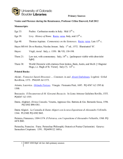
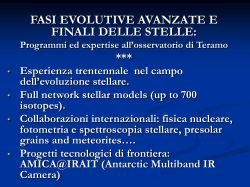
Geosci. Model Dev., 9, 431–450, 2016
www.geosci-model-dev.net/9/431/2016/
doi:10.5194/gmd-9-431-2016
© Author(s) 2016. CC Attribution 3.0 License.
FPLUME-1.0: An integral volcanic plume model accounting for ash
aggregation
A. Folch1 , A. Costa2 , and G. Macedonio3
1 CASE
Department, Barcelona Supercomputing Center, Barcelona, Spain
Nazionale di Geofisica e Vulcanologia, Sezione di Bologna, Bologna, Italy
3 Istituto Nazionale di Geofisica e Vulcanologia, Sezione di Napoli, Naples, Italy
2 Istituto
Correspondence to: A. Folch ([email protected])
Received: 22 July 2015 – Published in Geosci. Model Dev. Discuss.: 17 September 2015
Revised: 22 December 2015 – Accepted: 5 January 2016 – Published: 2 February 2016
Abstract. Eruption source parameters (ESP) characterizing
volcanic eruption plumes are crucial inputs for atmospheric
tephra dispersal models, used for hazard assessment and
risk mitigation. We present FPLUME-1.0, a steady-state 1-D
(one-dimensional) cross-section-averaged eruption column
model based on the buoyant plume theory (BPT). The model
accounts for plume bending by wind, entrainment of ambient
moisture, effects of water phase changes, particle fallout and
re-entrainment, a new parameterization for the air entrainment coefficients and a model for wet aggregation of ash particles in the presence of liquid water or ice. In the occurrence
of wet aggregation, the model predicts an effective grain size
distribution depleted in fines with respect to that erupted at
the vent. Given a wind profile, the model can be used to determine the column height from the eruption mass flow rate or
vice versa. The ultimate goal is to improve ash cloud dispersal forecasts by better constraining the ESP (column height,
eruption rate and vertical distribution of mass) and the effective particle grain size distribution resulting from eventual
wet aggregation within the plume. As test cases we apply the
model to the eruptive phase-B of the 4 April 1982 El Chichón
volcano eruption (México) and the 6 May 2010 Eyjafjallajökull eruption phase (Iceland). The modular structure of the
code facilitates the implementation in the future code versions of more quantitative ash aggregation parameterization
as further observations and experiment data will be available
for better constraining ash aggregation processes.
1
Introduction
Volcanic plumes (e.g. Sparks, 1997) are turbulent multiphase flows containing volcanic gas, entrained ambient air
and moisture and tephra, consisting on both juvenile (resulting from magma fragmentation), crystal and lithic (resulting
from wall rock erosion) particles ranging from metre-sized
blocks to micron-sized fine ash (diameter ≤ 63 µm). Sustained volcanic plumes present a negatively buoyant basal
thrust region where the mixture rises due to its momentum.
As ambient air is entrained by turbulent mixing, it heats and
expands, thereby reducing the average density of the mixture.
It leads to a transition to the convective region, in which positive buoyancy drives the mixture up to the so-called neutral
buoyancy level (NBL), where the mixture density equals that
of the surrounding atmosphere. Excess of momentum above
the NBL (overshooting) can drive the mixture higher forming
the umbrella region, where tephra disperses horizontally first
as a gravity current (e.g. Costa et al., 2013; Carazzo et al.,
2014) and then under passive wind advection forming a volcanic cloud (see Fig. 1).
Quantitative observations and models of volcanic plumes
are essential to provide realistic source terms to atmospheric
dispersal models, aimed at simulating atmospheric tephra
transport and/or the resulting fallout deposit (e.g. Folch,
2012). Plume models range in complexity from 1-D (onedimensional) integral models built upon the buoyant plume
theory (BPT) of Morton et al. (1956) to sophisticated multiphase Computational Fluid Dynamics (CFD) models (e.g.
Suzuki et al., 2005; Esposti Ongaro et al., 2007; Suzuki and
Koyaguchi, 2009; Herzog and Graf, 2010; Suzuki and Koyaguchi, 2013). The latter group of models are valuable to understand physical phenomena and the role of different param-
Published by Copernicus Publications on behalf of the European Geosciences Union.
432
A. Folch et al.: FPLUME-1.0
Total plume height
Gravity
current
Passive
transport
Umbrella
region
H_t
H_b
Neutral buoyancy level (NBL)
s
Particle
fallout
Particle
fallout
θ
Particle re-entrainment
Plume
axis
Wind
velocity
z
ua
Shear wind
entrainment
Convective
region
Wind
profile
Plume
axis
û
Plume cross
section
ua cos θ
θ
x
Vortex wind
entrainment
ua sin θ
g
Jet
region
Volcano
vent
Vent level
Sea level
Figure 1. Sketch of an axisymmetric volcanic plume raising in a wind profile. Three different regions (jet thrust, convective thrust and
umbrella) are indicated, with the convective region reaching a height Hb (that of the neutral buoyancy level), and the umbrella region raising
up to Ht above the sea level (a.s.l.). The inset plot details a plume cross section perpendicular to the plume axis, inclined of an angle θ with
respect to the horizontal.
eters but, given their high computational cost, coupling with
atmospheric dispersal models at an operational level is still
unpractical. Moreover, even sophisticated 3-D multiphase
models can have serious problems to accurately describe
the physical processes related to closure equations, computational spatial resolution, etc. For this reason, simpler 1D cross-section-averaged models or even empirical relationships between plume height and eruption rate (e.g. Mastin
et al., 2009; Degruyter and Bonadonna, 2012) are used in
practice to furnish eruption source parameters (ESP) to atmospheric transport models, the results of which strongly depend on the source term quantification (i.e. determination of
plume height, eruption rate, vertical distribution of mass and
particle grain size distribution).
Many plume models based on the BPT have been proposed after the seminal studies of Wilson (1976) and Sparks
(1986) to address different aspects of plume dynamics. For
example, Woods (1993) proposed a model to include the latent heat associated with condensation of water vapour and
quantify its effects upon the eruption column. Ernst et al.
(1996) presented a model considering particle sedimentation
and re-entrainment from plume margins. Bursik (2001) analysed how the interaction with wind enhances entrainment of
air, plume bending and decrease of the total plume height
for a given eruption rate. Several other plume models exist (see Costa et al., 2015, and references therein), considering different modelling approaches, simplifying assumptions
and model parameterizations. It is well recognized that the
Geosci. Model Dev., 9, 431–450, 2016
values of the air entrainment coefficients have a large influence on the results of the plume models. On the other hand,
volcanic ash aggregation (e.g. Brown et al., 2012) can occur
within the eruption column or, under certain circumstances,
downstream within the ash cloud (Durant et al., 2009). In
any case, the formation of ash aggregates (with typical sizes
around few hundreds of µm and less dense than the primary
particles) dramatically impacts particle transport dynamics
thereby reducing the atmospheric residence time of aggregating particles and promoting the premature fallout of fine
ash. As a result, atmospheric transport models neglecting aggregation tend to overestimate far-range ash cloud concentrations, leading to an overestimation of the risk posed by
ash clouds on civil aviation and an underestimation of ash
loading in the near field. So far, no plume model tries to predict the formation of ash aggregates in the eruptive column
and how it affects the particle grain size distribution erupted
at the vent. This can be explained in part because aggregation mechanisms are complex and not fully understood yet,
although theoretical models have been proposed for wet aggregation (Costa et al., 2010; Folch et al., 2010).
Here we present FPLUME-1.0, a steady-state 1-D crosssection-averaged plume model, which accounts for plume
bending, entrainment of ambient moisture, effects of water
phase changes on the energy budget, particle fallout and reentrainment by turbulent eddies, variable entrainment coefficients fitted from experiments and particle aggregation in
presence of liquid water or ice that depends on plume dy-
www.geosci-model-dev.net/9/431/2016/
A. Folch et al.: FPLUME-1.0
433
namics, particle properties, and amount of liquid water and
ice existing in the plume. The modelling of aggregation in
the plume, proposed here for the first time, allows our model
to predict an effective total grain size distribution (TGSD)
depleted in fines with respect to that erupted at the vent. The
ultimate goal is to improve ash cloud forecasts by better constraining these relevant aspects of the source term. In this
manuscript, we present first the governing equations for the
plume and aggregation models and then apply the combined
model to two test cases, the eruptive phase-B of the 1982 El
Chichón volcano eruption (México) and the 6 May 2010 Eyjafjallajökull eruption phase (Iceland).
Fig. 1) are the following (for the meaning of the used symbols see Tables 1 and 2):
2
P̂
Physical plume model
We consider a volcanic plume as a multiphase mixture of
volatiles, suspended particles (tephra) and entrained ambient
air. For simplicity, water (in vapour, liquid or ice phase) is
assumed the only volatile species, being either of magmatic
origin or incorporated through the ingestion of moist ambient
air. Erupted tephra particles can form by magma fragmentation or by erosion of the volcanic conduit, and can vary
notably in size, shape and density. For historical reasons,
field volcanologists describe the continuous spectrum of particle sizes in terms of the dimensionless 8-scale (Krumbein,
1934):
d(8) = d∗ 2−8 = d∗ e−8 log 2 ,
(1)
where d is the particle size and d∗ = 10−3 m is a reference length (i.e. 2−8 is the direction-averaged particle size
expressed in mm). The vast majority of modelling strategies, discretize the continuous particle grain size distribution
(GSD) by grouping particles in n different 8-bins, each with
an associated particle mass fraction (the models based on
moments (e.g. de’ Michieli Vitturi et al., 2015) are the exception). Because particle size exerts a primary control on
sedimentation, 8-classes are often identified with terminal
settling velocity classes although, strictly, a particle settling
velocity class is defined not only by particle size but also
by its density and shape. We propose a model for volcanic
plumes as a multiphase homogeneous mixture of water (in
any phase), entrained air, and n particle classes, including
a parameterization for the air entrainment coefficients and
a wet aggregation model. Because the governing equations
based upon the BPT are not adequate above NBL, we also
propose a new semi-empirical model to describe such a region.
2.1
Governing equations
The steady-state cross-section-averaged governing equations
for axisymmetric plume motion in a turbulent wind (see
www.geosci-model-dev.net/9/431/2016/
n
X
d M̂i
d M̂
= 2π rρa ue +
,
ds
ds
i=1
d P̂
= π r 2 ρa − ρ̂ g sin θ + ua cos θ (2π rρa ue )
ds
n
X
d M̂i
,
+ û
ds
i=1
dθ
= π r 2 ρa − ρ̂ g cos θ − ua sin θ (2π rρa ue ) ,
ds
(2a)
(2b)
(2c)
1
d Ê
= 2π rρa ue (1 − wa )ca Ta + wa hwa (Ta ) + gz + u2e
ds
2
n
X d M̂i
,
(2d)
+ cp T̂
ds
i=1
d M̂a
= 2π rρa ue (1 − wa ),
ds
(2e)
d M̂w
= 2π rρa ue wa ,
ds
(2f)
−1
d M̂i
χ usi
f ue
−
=−
1+
M̂i + A+
i − Ai ,
ds
r û
usi dr/ds
(2g)
dx
= cos θ cos 8a ,
ds
(2h)
dy
= cos θ sin 8a ,
ds
(2i)
dz
= sin θ,
ds
(2j)
where M̂ = π r 2 ρ̂ û is the total mass flow rate, P̂ = M̂ û is the
total axial (stream-wise) momentum flow rate, θ is the plume
bent over angle with respect to the horizontal (i.e. θ = 90◦ for
a plume raising vertically), Ê = M̂(Ĥ +gz+ 21 û2 ) is the total
energy flow rate, Ĥ is the enthalpy flow rate of the mixture,
T̂ = T̂ (Ĥ ) is the mixture temperature, M̂a is the mass flow
rate of dry air, M̂w = M̂ x̂w is the mass flow rate of volatiles
(including water vapour, liquid and ice), hwa is the enthalpy
Geosci. Model Dev., 9, 431–450, 2016
434
A. Folch et al.: FPLUME-1.0
Table 1. List of Latin symbols. Quantities with a hat denote bulk (top-hat averaged) quantities. Throughout the text, the subindex o (e.g. M̂o ,
ûo ) indicates values of quantities at the vent (s = 0).
Symbol
−
A+
i (Ai )
AB
ADS
AS
ATI
ca
cl
cp
cs
cv
Cd
Ĉi
Df
dA
di
el
es
Ê
fˆ
f
fi
g
hl
hs
hv
hl0
hs0
hv0
hwa
M̂
M̂a
M̂i
M̂w
Ni
ṅi
ṅtot
ntot
P̂
P
Pv
r
s
T̂
Ta
Tf
û
ua
ue
usi
wa
x
x̂l
x̂s
x̂v
x̂p
x̂w
y
z
zs
Definition
Units
Comments
Aggregation source (sink) terms
Collision frequency by Brownian motion
Collision frequency by differential sedimentation
Collision frequency by fluid shear
Collision frequency by turbulent inertia
Specific heat capacity of air at constant pressure
Specific heat capacity of liquid water
Specific heat capacity of particles (pyroclasts)
Specific heat capacity of solid water (ice)
Specific heat capacity of water vapour
Particle drag coefficient
Mass concentration of particles of class i
Fractal exponent
Diameter of the aggregates
Diameter of particles of class i
Saturation pressure of water vapour over liquid
Saturation pressure of water vapour over solid (ice)
Energy flow rate
Correction factor for aggregation
Particle re-entrainment parameter
Mass fraction of particle class i
Gravitational acceleration
Enthalpy per unit mass of liquid water
Enthalpy per unit mass of ice
Enthalpy per unit mass of vapour
Enthalpy per unit mass of liquid water at T = T0
Enthalpy per unit mass of ice at T = T0
Enthalpy per unit mass of vapour at T = T0
Enthalpy per unit mass of water in the atmosphere
Total mass flow rate
Mass flow rate of dry air
Mass flow rate of particles of class i
Mass flow rate of volatiles (water in any phase)
Number of particles of diameter di in an aggregate
Number of aggregating particles per unit volume and time
Total particle decay per unit volume and time
Number of particles per unit volume available for aggregation
Axial (stream-wise) momentum flow rate
Pressure
Partial pressure of water vapour
Cross section plume radius
Distance along the plume axis
Mixture temperature
Ambient air temperature
Freezing temperature
Mixture velocity along the plume axis
Horizontal wind (air) velocity
Air entrainment velocity (by turbulent eddies)
Terminal settling velocity of particle class i
Mass fraction of water in the entrained ambient air
Horizontal coordinate
Mass fraction of liquid water
Mass fraction of solid water (ice)
Mass fraction of water vapour
Mass fraction of particles (pyroclasts)
Mass fraction of volatiles (water)
Horizontal coordinate
Vertical coordinate
Dimensionless height
kgs−1 m−1
Given by Eqs. (28) and (29)
Given by Eq. (41a)
Given by Eq. (41c)
Given by Eq. (41b)
Given by Eq. (41d)
Default value 1000
Default value 4200
Default value 1600
Default value 2000
Default value 1900
Given by Eq. (15)
Given by Eq. (43)
Values between 2.8 and 3 (Costa et al., 2010)
One single aggregated class is assumed
Sphere equivalent diameter for irregular shapes
Given by Eq. (9)
Given by Eq. (10)
Ê = M̂(ĉT̂ + gz + 21 û2 )
See Appendix A. Values between 2-4.
Given
by Eq. (13)
P
fi = 1
Value of 9.81
Given by Eq. (6b)
Given by Eq. (6a)
Given by Eq. (6c)
Geosci. Model Dev., 9, 431–450, 2016
m3 s−1
m−1 s−1
s−1
m3 s−1
J kg−1 K−1
J kg−1 K−1
J kg−1 K−1
J kg−1 K−1
J kg−1 K−1
–
kgm−3
–
m
m
Pa
Pa
kg m2 s−3
–
–
–
ms−2
J kg−1
J kg−1
J kg−1
J kg−1
J kg−1
J kg−1
J kg−1
kg s−1
kg s−1
kg s−1
kg s−1
–
m−3 s−1
m−3 s−1
m−3
kg m s−2
Pa
Pa
m
m
K
K
K
ms−1
ms−1
ms−1
ms−1
–
m
–
–
–
–
–
m
m
–
See Eq. (2d)
P
M̂ = π r 2 ρ̂ û = M̂i + M̂w + M̂a
M̂i = M̂ x̂p fi
M̂w = M̂ x̂w
Given by Eq. (31)
Given by Eq. (30)
Given by Eq. (34)
Given by Eq. (42)
P̂ = M̂ û
Given by Eq. (8a)
Axial symmetry is assumed
Equations integrated from s = 0 to the NBL
Thermal equilibrium is assumed
Assumed to vary only with z
Value of 255 (-18C) assumed
Mechanical equilibrium is assumed
Assumed to vary only with z
Given by Eq. (17)
Given by Eq. (14)
Specific humidity (kg/kg)
Given by Eq. (4)
x̂w = x̂v + x̂l + x̂s
Typically given a.s.l. or a.v.l.
zs = z/2ro
www.geosci-model-dev.net/9/431/2016/
A. Folch et al.: FPLUME-1.0
435
Table 2. List of greek symbols. Quantities with a hat denote bulk (top-hat averaged) quantities.
Symbol
Definition
Units
Comments
αm
αij
αs
αv
0s
φ
µ̂
µl
ν̂
ρ̂
ρa
ρl
ρg
ρp
ρpi
ρs
φ
8
8a
9
θ
ξ
χ
Class-averaged particle sticking efficiency
Sticking efficiency between particles of class i and j
stream-wise (shear) air entrainment coefficient
cross-flow (vortex) air entrainment coefficient
Dissipation rate of turbulent kinetic energy
Fluid shear
Volume fraction of particles
Mixture dynamic viscosity
Liquid water dynamic viscosity
Mixture kinematic viscosity
Mixture density
Ambient air density
Liquid water density
Gas phase (dry air plus water vapour) density
Class-averaged particle (pyroclasts) density
Density of particles of class i
Ice density
Solid (particles) volume fraction
Dimensionless number related to size
Horizontal wind direction (azimuth)
Particle sphericity
Plume bent over angle with respect to the horizontal
Diameter to volume fractal relationship
Constant giving the probability of fallout
–
–
–
–
m2 s−3
s−1
–
Pa s
Pa s
m2 s−1
kg m−3
kg m−3
kg m−3
kg m−3
kg m−3
kg m−3
kg m−3
–
–
rad
–
rad
–
–
Given by Eq. (44)
Given by Eq. (45)
Given by Eq. (19)
Given by Eq. (21)
Given by Eq. (37)
Given by Eq. (39)
per unit mass of the water in the atmosphere, M̂i = M̂ x̂p fi is
the mass flow rate of particles of class i(i = 1 : n), x and y
are the horizontal coordinates, z is height and s is the distance
along the plume axis (see Tables 1 and 2 for the definition of
all symbols and variables appearing in the manuscript).
The equations above derive from conservation principles assuming axial (stream-wise) symmetry and considering bulk quantities integrated over a plume cross section using a top-hat profile in which a generic quantity φ has a
constant value φ̂(s) at a given plume cross section and vanishes outside (here we refer to section-averaged quantities
as bulk quantities, denoted by a hat). We have derived these
equations by combining formulations from different previous plume models (Netterville, 1990; Woods, 1993; Ernst
et al., 1996; Bursik, 2001; Costa et al., 2006; Woodhouse
et al., 2013) in order to include in a single model effects from
plume bending by wind, particle fallout and re-entrainment
at plume margins, transport of volatiles (water) accounting
also for ingestion of ambient moisture, phase changes (water
vapour condensation and deposition) and particle aggregation. Equation (2j) expresses the conservation of total mass,
accounting in the right-hand side (rhs) for the mass of air
entrained through the plume margins and the loss/gain of
mass by particle fallout/re-entrainment. Equation (2b) and
(2c) express the conservation of axial (stream-wise) and radial momentum, respectively, accounting on the rhs for con-
www.geosci-model-dev.net/9/431/2016/
Assumed equal to that of air at bulk temperature
ν̂ = µ̂/ρ̂
Given by Eq. (3)
Assumed to vary only with z
Value of 1000
ρp =
P
fi ρpi
Value of 920
P
φ = Ĉi / ρpi
Given by Eq. (1)
9 = 1 for spheres
Value of ≈ 0.23(Bursik, 2001)
tributions from buoyancy (first term), entrainment of air, and
particle fallout/re-entrainment. Note that generally the buoyancy term, acting only along the vertical direction z, represents a sink of momentum in the basal gas-thrust jet region
(where ρ̂ > ρa ) and a source of momentum where the plume
is positively buoyant (ρ̂ < ρa ). Equation (2d) expresses the
conservation of energy, accounting on the rhs for gain of energy (enthalpy, potential and kinetic) by ambient air entrainment (first term), loss/gain by particle fallout/re-entrainment
(second term), and gain of energy by conversion of water
vapour into liquid (condensation) or into ice (deposition).
Equation (2e), (2f) and (2g) express, respectively, the conservation of mass of dry air, water (vapour, liquid and ice) and
solid particles. The latter set of equations, one for each particle class, account on the rhs for particle re-entrainment (first
term), particle fallout (second term) and particle aggregation.
−
Here we have included to terms (A+
i and Ai ) that account for
the creation of mass from smaller particles aggregating into
particle class i and for the destruction of mass resulting from
particles of class i contributing to the formation of largersize aggregates. Finally, Eq. (2h) to (2j) determine the 3-D
plume trajectory as a function of the length parameter s. All
these equations constitute a set of 9 + n first order ordinary
differential equations in s for 9 + n unknowns: M̂, P̂ , θ , Ê,
M̂a , Mˆw , M̂i (for each particle class), x, y and z. Note that,
Geosci. Model Dev., 9, 431–450, 2016
436
A. Folch et al.: FPLUME-1.0
using the definitions of M̂-P̂ -Ê, the equations can also be
expressed in terms of û-r-T̂ given the bulk density.
Assuming an homogeneous mixture, the bulk density ρ̂ of
the mixture is
x̂p x̂l x̂s (1 − x̂p − x̂l − x̂s )
1
=
+ + +
,
ρ̂
ρp ρl ρs
ρg
The model uses a pseudo-gas assumption considering that
the mixture of air and water vapour behaves as an ideal gas:
P = Pv + Pa ;
where x̂p , x̂l and x̂s are, respectively, the mass fractions of
particles, liquid water and ice, ρp is the class-weighted average density of particles (pyroclasts), ρl and ρs are liquid
water and ice densities, and ρg is the gas phase (i.e. dry air
plus water vapour) density. Under the assumption of mechanical equilibrium (i.e. assuming the same bulk velocity û for
all phases and components) it holds that
P
P
M̂i
M̂i
=P
.
(4)
x̂p =
M̂
M̂i + M̂w + M̂a
The enthalpy flow rate of the mixture is a non-decreasing
function of the temperature T̂ given by
Ĥ = M̂[xa ca T̂ +xp cp T̂ +xv hv (T̂ )+xl hl (T̂ )+xs hs (T̂ )], (5)
where hv , hl and hs are, respectively, the enthalpy per unit
mass of water vapour, liquid and ice:
hs (T̂ ) = cs T̂ ,
(6a)
hl (T̂ ) = hl0 + cl (T̂ − T0 ),
(6b)
(6c)
where cs =2108 J K−1 kg−1 is the specific heat of ice, T0 is
a reference temperature, hl0 =3.337×105 J kg−1 is the enthalpy of the liquid water at the reference temperature, cl =
4187 J K−1 kg−1 is the specific heat of liquid water, hv0 =
2.501×106 J kg−1 is the enthalpy of vapour water at the reference temperature and cv =1996 J K−1 kg−1 is the specific
heat of vapour water. For convenience, the reference temperature T0 is taken equal to the temperature of triple point of
the water (T0 = 273.15 K). The energy and the enthalpy flow
rate are related by
1
Ê = Ĥ + M̂(gz + u2 ).
2
(7)
For the integration of Eq. (2d) and for evaluating the aggregation rate terms in Eq. (2g), the temperature T̂ and the mass
fractions of ice (xs ), liquid water (xl ) and vapour (xv ) need
to be evaluated. These quantities are obtained by the direct
inversion of Eq. (5), with the use of Eqs. (2d) and (7) and by
assuming that the pressure inside the plume P is equal to the
atmospheric pressure at the same altitude (z).
Geosci. Model Dev., 9, 431–450, 2016
P a = na P ,
(8a)
xa /ma
,
xv /mv + xa /ma
(8b)
(3)
nv =
hv (T̂ ) = hv0 + cv (T̂ − T0 ),
Pv = nv P ;
xv /mv
;
xv /mv + xa /ma
na =
where Pv and Pa are, respectively, the partial pressures of the
water vapour and of the air in the plume, nv and na are the
molar fractions of vapour and air in the gas phase (nv + na =
1) and mv = 0.018 kg/mole and ma = 0.029 kg/mole are the
molar weights of vapour and air. Following Woods (1993)
and Woodhouse et al. (2013), we consider that, if the airwater mixture becomes saturated in water vapour, condensation or deposition occurs and the plume remains just saturated. This assumption implies that the partial pressure of
water vapour Pv equals the saturation pressure of vapour over
liquid (el ) or over ice (es ) at the bulk temperature, and the
saturation pressures over liquid and ice are given (in hPa) by
(Murphy and Koop, 2005)
!
T̂ − 273.16
(9)
el = 6.112 exp 17.67
T̂ − 29.65
273.16
273.16
log es = −9.097(
− 1) − 3.566 log(
),
T̂
T̂
T̂
) + log(6.1071).
(10)
+ 0.876(1 −
273.16
Equation (9) holds for T̂ ≥ Tf and Eq. (10) is valid for T̂ ≤
Tf , where Tf is the temperature of the triple point of the
water (here set at Pf = 611.2 Pa, Tf = 273.16 K). Therefore,
if T̂ > Tf and Pv < el , the plume is undersaturated and there
is no water vapour condensation (i.e. x̂v = x̂w and x̂l = x̂s =
0). In contrast, if Pv ≥ el , the vapour in excess is immediately
converted into liquid and
(P − el ) nv = el na
x̂s = 0
x̂l = x̂w − x̂v .
(11)
The vapour and air mass fractions xv and xa are evaluated
by combining Eq. (11) and (8b). On the other hand, if T̂ ≤
Tf and Pv < es the plume is undersaturated and there is no
water vapour deposition. In contrast, if Pv ≥ es , the vapour
in excess is immediately converted into ice and
(P − es ) nv = es na
x̂l = 0
x̂s = x̂w − x̂v .
(12)
Again, the vapour and air mass fractions xv and xa are evaluated by combining Eq. (12) and (8b).
www.geosci-model-dev.net/9/431/2016/
A. Folch et al.: FPLUME-1.0
437
For the particle re-entrainment parameter f we adopt the
fit proposed by Ernst et al. (1996) using data for plumes not
affected by wind:

"
# −1
1/4 6
0.78u
P
s o
 ,
f = 0.431 +
(13)
1/2
Fo
where Po = ro2 û2o and Fo = ro2 ûo Ĥo are the specific momentum and thermal fluxes at the vent (s =0), and Ĥo is the enthalpy per unit mass of the mixture at the vent. This expression may overestimate re-entrainment for bent over plumes
(Bursik, 2001). Finally, particle terminal settling velocity usi
is parameterized as (Costa et al., 2006; Folch et al., 2009)
s
4g(ρpi − ρ̂)di
,
(14)
usi =
3Cd ρ̂
where di is the class particle diameter and Cd is a drag coefficient that depends on the Reynolds number Re = di usi ρ̂ / µ̂.
Several empirical fits exist for drag coefficients of spherical
and non-spherical particles (e.g. Wilson and Huang, 1979;
Arastoopour et al., 1982; Ganser, 1993; Dellino et al., 2005).
In particular, Ganser (1993) gave a fit valid over a wide range
of particle sizes and shapes covering the spectrum of volcanic
particles considered in volcanic column models (lapilli and
ash):
o
24 n
Cd =
1 + 0.1118[Re (K1 K2 )]0.6567
ReK1
0.4305K2
+
,
(15)
3305
1 + ReK
K
1 2
where K1 and K2 are two shape factors depending on particle sphericity, 9, and particle orientation. Given that the
Cd depends on Re (i.e. on us ), Eq. 14 is solved iteratively
using a bisection algorithm. Given a closure equation for
the turbulent air entrainment velocity ue , and an aggregation model (defining the mass aggregation coefficients A+
i
and A−
i ), Eq. (2j) to (2i) can be integrated along the plume
axis from the inlet (volcanic vent) up to the neutral buoyancy level. Inflow (boundary) conditions are required at the
vent (s = 0) for, e.g., total mass flow rate M̂o , bent over angle
θo = 90◦ , temperature T̂o , exit velocity ûo , fraction of water
x̂wo , null air mass flow rate M̂a = 0, vent coordinates (xo ,yo
and zo ), and mass flow rate for each particle class M̂io . The
latter is obtained from the total mass flow rate at inflow given
the particle grain size distribution at the vent:
M̂io = fio M̂o (1 − x̂wo ),
(16)
where fio is the mass fraction of class i at the vent.
2.2
Entrainment coefficients
Turbulent entrainment of ambient air plays a key role on the
dynamics of jets and buoyant plumes. In the basal region of
www.geosci-model-dev.net/9/431/2016/
volcanic columns, the rate of entrainment dictates whether
the volcanic jet enters into a collapse regime by exhaustion of
momentum before the mixture becomes positively buoyant,
or whether it evolves into a convective regime reaching much
higher altitudes. Early laboratory experiments (e.g. Hewett
et al., 1971) already indicated that the velocity of entrainment
of ambient air is proportional to velocity differences parallel
and normal to the plume axis (see inset in Fig. 1):
ue = αs |û − ua cos θ | + αv |ua sin θ |,
(17)
where αs and αv are dimensionless coefficients that control the entrainment along the stream-wise (shear) and crossflow (vortex) directions, respectively. Note that, in absence
of wind (i.e. ua = 0), the equation above reduces to ue = αs û
and the classical expression for entrainment velocity of Morton et al. (1956) is recovered. In contrast, under a wind field,
both along-plume (proportional to the relative velocity differences parallel to the plume) and cross-flow (proportional to
the wind normal component) contributions appear. However
it is worth noting that Eq. (17) has not a solid theoretical justification and is used on an empirical basis. A vast literature
exists regarding the experimental (e.g. Dellino et al., 2014)
and numerical (e.g. Suzuki and Koyaguchi, 2009) determination of entrainment coefficients for jets and buoyant plumes.
Based on these results, most 1-D integral plume models
available in literature consider (i) same constant entrainment
coefficients along the plume, (ii) piecewise constant values
at the different regions
p or, (iii) piecewise constant values corrected by a factor ρ̂/ρa (Woods, 1993). Typical values for
the entrainment coefficients derived from experiments are
of the order of αs ≈ 0.07–0.1 for the jet region, αs ≈ 0.1–
0.17 for the buoyant region and αv ≈ 0.3–1.0 (e.g. Devenish,
2013). However, more recent experimental (Kaminski et al.,
2005) and sensitivity analysis numerical studies (Charpentier and Espíndola, 2005) concluded that piecewise constant
functions are valid only as a first approach, implying that
1-D integral models assuming constant entrainment coefficients do not always provide satisfactory results. This has
also been corroborated by 3-D numerical simulations of volcanic plumes (Suzuki and Koyaguchi, 2013), which indicate
that 1-D integral models overestimate the effects of wind on
turbulent mixing efficiency (i.e. the value of αv ) and, consequently, underestimate plume heights under strong wind
fields. For example, recent 3-D numerical simulation results
for small-scale eruptions under strong wind fields suggest
lower values of αv , in the range 0.1–0.3 (Suzuki and Koyaguchi, 2015). For this reason, besides the option of constant entrainment coefficients, FPLUME allows for considering also a parameterization of αs and αv based on the local
Richardson number. In particular, we use the empirical parameterization of Kaminski et al. (2005) and Carazzo et al.
(2006, 2008a, b) that describes αs for jets and plumes as a
function of the local Richardson number as
1
r 1 dA
αs = 0.0675 + 1 −
Ri +
,
(18)
A(zs )
2 A(zs ) dz
Geosci. Model Dev., 9, 431–450, 2016
438
A. Folch et al.: FPLUME-1.0
Moreover, in order to use a compact analytical expression
and extend it to values of zs ≤ 10 we fitted the experimental
data of Carazzo et al. (2006, 2008b) considering the following empirical function:
zs2 + c1
,
(20a)
A(zs ) = co 2
zs + c2
1 dA
1
2 (c2 − c1 )zs
,
=
A(zs ) dz
2r0 zs2 + c1 zs2 + c2
(20b)
and in order to extrapolate to low zs we multiply A(zs ) for
the following function h(zs ) that affects the behaviour only
for small values of zs :
h(zs ) =
1
,
1 − c4 exp (−5 (zs /10 − 1))
(20c)
where ci are dimensionless fitting constants. Best-fit results
and entrainment functions resulting from fitting Eq. (20a)–
(20c) are shown in Table 3 and Fig. 2, respectively. However,
the veracity of the empirical parameterization in Eq. (18) was
not observed by Wang and Wing-Keung Law (2002) in their
experiments nor has it been seen in Direct Numerical Simulation (DNS) or Large Eddy Simulations (LES) simulations
of buoyant plumes (e.g. Craske et al., 2015). Finally, for the
vortex entrainment coefficient αv , we adopt a parameterization proposed by Tate (2002) based on a few laboratory experiments:
αv = 0.34
p
ūa
2|Ri|
ûo
−0.125
,
(21)
where ûo is the mixture velocity at the vent and ūa is the average wind velocity. For illustrative purposes, Fig. 3 shows
the entrainment coefficients αs and αv predicted by Eqs. (19)
and (21) for weak and strong plume cases under a prescribed
wind profile. It is important stressing that air entrainment
rates play a first-order role on eruptive plume dynamics and a
simple description in terms of entrainment coefficients, both
assuming them as empirical constants or describing them
like in Eq. (18), represents an over-simplification of the real
physics characterizing the processes. A better quantification
of entrainment rates is one of the current main challenges of
the volcanological community (see Costa et al., 2015, and
references therein).
Geosci. Model Dev., 9, 431–450, 2016
2
Jet
Plume
1.9
1.8
1.7
Entrainment function A
where A(zs ) is an entrainment function depending on the
dimensionless length zs = z/2ro (ro is the vent radius) and
Ri = g(ρa − ρ̂)r/ρa û2 is the Richardson number. Beside the
local Richardson number, the entrainment coefficient αs depends on plume orientation (e.g. Lee and Cheung, 1990; Bemporad, 1994), therefore we modify Eq. 18 as:
r 1 dA
1
Ri sin θ +
αs = 0.0675 + 1 −
. (19)
A(zs )
2 A(zs ) dz
1.6
1.5
1.4
1.3
1.2
1.1
1
0.1
1
10
Dimensionless height z_s
100
Figure 2. Entrainment functions A(zs ) for jets and plumes depending on the dimensionless height zs = z/2ro . Functions have been
obtained by fitting experimental data (points) from Carazzo et al.
(2006) (for zs > 10) and multiplying by a correction function (20c)
to extend the functions to zs < 10 verifying function continuity and
convergence to values of A = 1.11 for jets and A = 1.31 for plumes
when zs → 0.
Table 3. Constants defining the entrainment functions for jets and
plumes following the formulation introduced by Kaminski et al.
(2005) (see Eq. 20a to 20c) obtained after fitting experimental data
reported in Carazzo et al. (2006). For Kaminski-R we considered all
data including that of Rouse et al. (1952), whereas for Kaminski-C,
as suggested by Carazzo et al. (2006), data from Rouse et al. (1952)
was excluded.
Kaminski-R
jets
plumes
c0
c1
c2
c3 = 2(c2 − c1 )
c4
2.3
1.92
3737.26
4825.98
2177.44
0.00235
1.61717
478.374
738.348
519.948
-0.00145
Kaminski-C
jets
plumes
1.92
3737.26
4825.98
1883.81
0.00235
1.55
329.0
504.5
351.0
−0.00145
Modelling of the umbrella region
The umbrella region is defined as the upper region of the
plume, from about the NBL to the top of the column. This region can be dominated by fountaining processes of the eruptive mixture that reaches the top of the column, dissipating
the excess of momentum at the NBL, and then collapsing as
a gravity current (e.g. Woods and Kienle, 1994; Costa et al.,
2013). The 1-D BPT should not be extended to this region
because it assumes that the mixture still entrains air with the
same mechanisms as below NBL and, moreover, predicts that
the radius goes to infinity towards the top of the column. For
these reasons, we describe the umbrella region adopting a
simple semi-empirical approximation.
In the umbrella region (from the NBL to the top of the column), we neglect air entrainment and assume that the mixwww.geosci-model-dev.net/9/431/2016/
A. Folch et al.: FPLUME-1.0
439
ture is homogeneous, i.e. the content of air, water vapour,
liquid water, ice and total mass of particles do not vary with
z. Pressure P (z) is considered equal to the atmospheric pressure Pa (z) evaluated at the same level, whereas temperature
decreases with z due to the adiabatic cooling:
P (z) = Pa (z) and
1
dT
=
.
dP
ĉρ̂
(22)
As a consequence, the density of the mixture varies accordingly. The total height of the volcanic plume Ht , above the
vent, is approximated as (e.g. Sparks, 1986)
Ht = cH (Hb + 8ro ),
(23)
where cH is a dimensionless parameter (typically cH =
1.32), Hb is the height of the neutral buoyancy level (above
the vent) and ro the radius at the vent. Between Hb and Ht ,
the coordinates x and y of the position of the plume centre
and the plume radius r are parameterized as a function of
the elevation z, with Hb ≤ z ≤ Ht . The position of the plume
centre is assumed to vary linearly with the same slope at the
NBL, whereas the effective plume radius is assumed to decrease as a Gaussian function:
dx ,
(24)
x = xb + (z − Hb ) dz z=zb
dy y = yb + (z − Hb ) ,
(25)
dz
z=zb
r = rb e
−(z−Hb )2 /2σH2
,
(26)
where xb , yb , rb are, respectively, the coordinates x and y of
the centre of the plume and the plume radius at the NBL, and
σH = Ht − Hb .
Finally, assuming that the kinetic energy of the mixture is
converted to potential energy, the vertical velocity is approximated to decrease as the square root of the distance from the
NBL:
s
Ht − z
uz = uzb
,
(27)
Ht − Hb
where uzb is the vertical velocity of the plume at the NBL.
Although the proposed empirical parameterization of the region above the NBL is qualitatively consistent with the trends
predicted by 3-D numerical models (Costa et al., 2015), a
more rigorous description requires further research.
3
Plume wet aggregation model
Particle aggregation can occur inside the column or in the ash
cloud during subsequent atmospheric dispersion (e.g. Carey
and Sigurdsson, 1982; Durant et al., 2009), thereby affecting
the sedimentation dynamics and deposition of volcanic ash.
Our model explicitly accounts for aggregation in the plume
www.geosci-model-dev.net/9/431/2016/
−
by adding source (A+
i ) and sink (Ai ) terms for aggregates
and aggregated particles in their respective particle mass balance Eqs. (2g) and by modifying the settling velocity of aggregates. Given the complexity of aggregation phenomena,
not yet fully understood, we consider only the occurrence
of wet aggregation and neglect dry aggregation mechanisms
driven by electrostatic forces or disaggregation processes resulting from particle collisions that can break and decompose aggregates. Costa et al. (2010) and Folch et al. (2010)
proposed a simplified wet aggregation model in which particles aggregate on a single effective aggregated class characterized by a diameter dA (i.e. aggregation only involves
particle classes having an effective diameter smaller than dA ,
typically in the range 100–300 µm). Obviously the assumption that all particles aggregate into a single particle class
is simplistic and considering a range of aggregating classes
would be more realistic. However, there are no quantitative
data available for such a calibration. Hence, considering this
assumption it follows that
A+
i =
n
X
A−
j δik ,
(28)
j =k+1
where k is the (given) index of the aggregated class and the
sum over j spans all particle classes having diameters lower
than dA . The mass of particles of class i (di < dA ) that aggregate per unit of time and length in a given plume cross
section is
π (29)
A−
=
ṅ
ρpi di3 π r 2 ,
i
i
6
where ṅi is the number of particles of class i that aggregate
per unit volume and time, estimated as
ṅtot Ni
ṅi ≈ P .
Nj
(30)
In the expression above, Ni is the number of particles of
diameter di in an aggregate of diameter dA , and ṅtot is the
total particle decay per unit volume and time. Costa et al.
(2010) considered that Ni is given by a semi-empirical fractal
relationship (e.g. Jullien and Botet, 1987; Frenklach, 2002;
Xiong and Friedlander, 2001):
Ni = kf
dA
di
Df
,
(31)
where kf is a fractal pre-factor and Df is the fractal exponent. Costa et al. (2010) and Folch et al. (2010) assumed
constant values for kf and Df that were calibrated by bestfitting tephra deposits from 18 May 1980 Mount St. Helens
and 17–18 September 1992 Crater Peak eruptions. However,
for the granulometric data from these deposits they used a
cut-off considering only particles larger than about 10µm, for
which the gravitational aggregation kernel dominates. This
poses a problem if one wants to extend the granulometric
Geosci. Model Dev., 9, 431–450, 2016
440
A. Folch et al.: FPLUME-1.0
distribution to include micrometric and sub-micrometric particles, for which the Brownian kernel is the dominant one
(it is known that Brownian particle–particle interaction has
typical values of Df ≈ 2, with values ranging between 1.5
and 2.5, e.g. Xiong and Friedlander, 2001). Actually, preliminary model tests involving micrometric and sub-micrometric
particle classes considering constant values for Df and kf
have revealed a strong dependency of results (fraction of aggregated mass) on both granulometric cut-off and bin width
(particle grain size discretization). In order to overcome this
problem, we assume a size-dependent fractal exponent as
Df 2
) − 0.228
2
2.5
60
2
40
Plume region
1.5
1
20
(32)
0
#Df 2 + Df
Df
0
0.1
Jet region
0.3
0.4
0.5
0.6
0.7
Entrainment coefficients
0.2
30
0.8
0.9
1
1.1
0
35
a_s
a_v
!%#$
25
30
Umbrella region
Df /2
.
25
20
20
15
15
10
Plume region
10
(33)
5
Figure 4 shows the values of Df (d) and kf (d) predicted by
Eqs. (32) and (33) for a range of Df o . We have performed
different tests to verify that, in this way, the results of the
aggregation model become much more robust independently
of the distribution cut-off (8min = 8, 10, 12) and bin width
(18 = 1, 0.5, 0.25), with maximum differences in the aggregated mass laying always below 10 %.
The total particle decay per unit volume and time ṅtot is
given by
2−4 / Df
ṅtot = fˆαm (AB n2tot + ATI φ 4 / Df ntot
2−3/Df
+ AS φ 3 / Df ntot
2−4 / Df
+ ADS φ 4 / Df ntot
),
(34)
where αm is a mean (class-averaged) sticking efficiency, φ
is the solid volume fraction, ntot is the total number of particles per unit of volume that can potentially aggregate and
fˆ is a correction factor that accounts for conversion from
Gaussian to top-hat formalism (see Appendix A for details).
The expression above comes from integrating the collection
kernel over all particle sizes, and involves the product of the
(averaged) sticking efficiency times the collision frequency
function accounting for Brownian motion (AB ), collision due
to turbulence as a result of inertial effects (ATI ), laminar
and turbulent fluid shear (AS ), and differential sedimentation
(ADS ). The term AB derives from the Brownian collision kernel βB,ij (Costa et al., 2010):
βB,ij =
2kb T̂ (di + dj )2
,
3µ̂
dj dj
Geosci. Model Dev., 9, 431–450, 2016
Height (km a.v.l.)
Dimensionless height z_s
3
(35)
Height (km a.v.l.)
1.56 − (1.728 −
3.5
80
where Df o ≤ 3, Dmin = 1.6, dµ ≈ 2µm and a = 1.36788.
The values of Dmin and dµ represent, respectively, the minimum value of Df relevant for sub-micrometric particles and
the scale below which the Brownian aggregation kernel becomes dominant. For the fractal pre-factor kf we adopt the
expression of Gmachowski (2002):
kf =
Umbrella region
0.5
a (Dfo − Dmin )
,
1 + exp((d − dµ ) / dµ )
"r
4
a_s
a_v
!"#$
Dimensionless height z_s
Df (d) = Dfo −
100
5
Jet region
0
0
0.1
0.2
0.3
0.4
0.5
0.6
0.7
0.8
0.9
1
1.1
0
Entrainment coefficients
Figure 3. Entrainment coefficients αs (red) and αv (blue) versus
height for weak (a) and strong (b) plumes under a wind profile.
The vertical dashed lines indicate the transition between the different eruptive column regions. Weak plume simulation with: M̂o =
1.5×106 kgs−1 , ûo = 135 ms−1 , T̂o = 1273 K, x̂wo = 0.03. Strong
plume simulation with: M̂o = 1.5 × 109 kg s−1 , ûo = 300 ms−1 ,
T̂o = 1153 K, x̂wo = 0.05.
where kb is the Boltzmann constant and µ̂ is the mixture dynamic viscosity (≈ air viscosity at the bulk temperature T̂ ).
The term ATI derives from the collision kernel due to turbulence as result of inertial effects βTI,ij (e.g. Pruppacher and
Klett, 1996; Jacobson, 2005):
βTI,ij =
3/4 π
(di + dj )2 |usj − usi |,
g ν̂ 1/4 4
(36)
where ν̂ is the mixture kinematic viscosity and is the dissipation rate of turbulent kinetic energy, computed assuming
the Smagorinsky–Lilly model:
√
û3
= 2 2ks2 ,
r
(37)
where ks ≈ 0.1 − 0.2 is the constant of Smagorinsky. The
term AS derives from the collision kernel due to laminar and
www.geosci-model-dev.net/9/431/2016/
A. Folch et al.: FPLUME-1.0
441
turbulent fluid shear βS,ij (Costa et al., 2010):
βS,ij =
3
0S
di + dj ,
6
where 0S is the fluid shear, computed as
d û 1/2
0S = max ,
.
dr
ν
(38)
(39)
Finally, the term ADS derives from the differential sedimentation collision kernel βDS,ij (e.g. Costa et al., 2010):
βDS,ij
π
= (di + dj )2 |usi − usj |,
4
(40)
(41a)
2
A S = − 0S ξ 3 ,
3
(41b)
π(ρp − ρ̂)gξ 4
,
48µ̂
(41c)
3/4
ADS ,
gν 1/4
(41d)
−1/D
f
where ξ = dj vj
is the diameter to volume fractal relationship and vj is the particle volume. Note that for spherical
particles in the Euclidean space (Df = 3) vj = π dj3 /6 and
ξ = (6/π )1/3 .
The total number of particles per unit of volume available
for aggregation is related to particle class mass concentration
at each section of the plume Ĉj and can be estimated as (see
Appendix B)
!"
#
6Ĉj
1 X
1
1
ntot =
− 3 ,
(42)
3
3 log 2 j
π 18j ρpj
daj
dbj
where daj and dbj are the particle diameters of the limits of
the interval j and
Ĉj = ρ̂
M̂j
M̂
1
,
1 + (Stij / Stcr )q
.
www.geosci-model-dev.net/9/431/2016/
(43)
(45)
where Stcr = 1.3 is the critical Stokes number, q = 0.8 is a
constant, and Stij is the Stokes number based on the binder
liquid (water) viscosity:
Stij =
8ρ̂ di dj
|ui − uj |,
9µl di + dj
(46)
where
|ui − uj | = |usi − usj | +
4kb T̂
,
AB = −
3µ̂
ATI = 1.82
where fk is the particle class mass fraction, and αij is the
sticking efficiency between the classes i and j . In presence of
a pure ice phase we assume that ash particles stick as ice particles (αm = 0.09). In contrast, in presence of a liquid phase,
the aggregation model considers
αij =
where usi denotes the settling velocity of particle class i.
Note that, with respect to the original formulation of Costa
et al. (2010), using the same approach and approximation,
we have included the additional term ATI due to the turbulent
inertial kernel that, thanks to the similarity between Eqs. (40)
and (36), can be easily derived. Once these kernels are integrated, expressions for the terms in Eq. (34) yield
ADS = −
Finally, the class-averaged sticking efficiency αm appearing
in Eq. (34) is computed as
PP
i
j fi fj αij
αm = P P
,
(44)
i
j fi fj
20s (di + dj )
8kb T̂
.
+
3µ̂π di dj
3π
(47)
Obviously, our aggregation model requires the presence of
water either in liquid or solid phases, i.e. aggregation will
only occur in those regions of the plume where water vapour
(of magmatic origin or entrained by moist air) meets condensation/deposition conditions (Costa et al., 2010; Folch
et al., 2010). This depends on complex relationships between plume dynamics and ambient conditions. For highintensity (strong) plumes having high values of M̂, the condition Pv ≥ el when T̂ > Tf is rarely met, implying no formation of a liquid water window within the plume. Aggregation occurs in this case only at the upper parts of the column, under the presence of ice. In contrast, lower-intensity
(weak) plumes having lower values of M̂ can form a liquid
water window if the term Ma dominates in Eq. (8a). However, this also depends on a complex balance between air entrainment efficiency, ambient moisture, plume temperature,
height level, cooling rate and ambient conditions. Aggregation by liquid water is much favoured under moist environments and by efficient air entrainment. Note that, keeping all
eruptive parameters constant, the occurrence (or not) of wet
aggregation by liquid water can vary with time depending on
fluctuations of the atmospheric moisture and wind intensity
along the day.
4
FPLUME-1.0
We solve the model equations using FPLUME-1.0, a code
written in FORTRAN90 that uses the lsode library (Hindmarsh, 1980), to solve the set of first-order ordinary differential equations. Model inputs are eruption start and duration (different successive eruption phases can be considered),
Geosci. Model Dev., 9, 431–450, 2016
442
vent coordinates (xo ,yo ) and elevation (zo ), conditions at the
vent (exit velocity ûo , magma temperature T̂o , magmatic water mass fraction ŵo , and total grain size distribution) and
total column height Ht or mass eruption rate M̂o . The code
has two solving modes. If M̂o is given, the code solves directly for Ht . On the contrary, if Ht is given, the code solves
iteratively for M̂. Wind profiles can be furnished in different
formats, including standard atmosphere, atmospheric soundings, and profiles extracted from meteorological re-analysis
data sets. If the aggregation model is switched on, additional
inputs are required including size and density of the aggregated class, aggregates settling velocity factor (to account for
the decrease in settling velocity of aggregates due to increase
in porosity), and fractal exponent for coarse particles Df o .
The rest of the parameters (specific heats, the value of the
constant χ for particle fallout probability, parameterization
of the entrainment coefficients, etc.) have assigned default
values but can be modified by the user using a configure file.
Model outputs include a text file with the results for each
eruption phase giving values of all computed variables (e.g.
û, T̂ , ρ̂) at different heights, and a file giving the mass flow
rate of each particle class that falls from the column at different heights (cross sections). This file provides the phasedependent source term, and hence serves to couple FPLUME
with atmospheric dispersion models. In case of wet aggregation, the effective granulometry predicted by the aggregation model is also provided. The solution of the aggregation
model embedded in FPLUME-1.0 consists on the following
steps:
1. At each section of the plume, determine the water
vapour condensation or deposition conditions depending on T̂ and Pv using Eqs. (11) or (12), respectively.
2. In case of saturation or deposition, compute the classaveraged sticking efficiency αm for liquid water or ice
using Eq. (44).
3. Estimate the total number of particles per unit of volume available for aggregation ntot depending on Cˆj using Eq. (42).
4. Compute the integrated aggregation kernels using
Eq. (41a) to (41d).
5. Compute the total particle decay per unit volume and
time ṅtot using Eq. (34) depending also on the solid volume fraction.
6. Compute the number of particles of diameter di in an
aggregate of given diameter dA using Eq. (31) assuming
size-dependent fractal exponent Df and pre-factor kf .
7. Compute class particle decay ṅi using Eq. (30).
8. Finally, compute the mass sink term for each aggregating class A−
i using Eq. (29) and the mass source term
A+
for
the
aggregated
class using Eq. (28) to introduce
i
Geosci. Model Dev., 9, 431–450, 2016
A. Folch et al.: FPLUME-1.0
these terms in the particle class mass balance equations,
Eq. (2g).
5
Test cases
As we mentioned above, here we apply FPLUME to two
eruptions relatively well characterized by previous studies.
In particular we consider the strong plume formed during
4 April 1982 by El Chichón 1982 eruption (e.g. Sigurdsson et al., 1984; Bonasia et al., 2012) and the weak plume
formed during the 6 May 2010 Eyjafjallajökull eruption (e.g.
Bonadonna et al., 2011; Folch, 2012).
5.1
Phase-B El Chichón 1982 eruption
El Chichón volcano reawakened in 1982 with three significant Plinian episodes occurring during March 29th (phase
A) and April 4th (phases B and C). Here we focus on the
second major event, starting at 01:35 UTC on April 4th and
lasting nearly 4.5 h (Sigurdsson et al., 1984). Bonasia et al.
(2012) used analytical (HAZMAP) and numerical (FALL3D)
tephra transport models to reconstruct ground deposit observations for the three main eruption fallout units. Deposit bestfit inversion results for phase-B suggested column heights
between 28 and 32 km (above vent level, a.v.l.) and a total
erupted mass ranging between 2.2 × 1012 and 3.7 × 1012 kg.
Considering a duration of 4.5 h, the resulting averaged mass
eruption rates are between 1×108 and 2.3×108 kg/s. TGSD
of phases B and C were estimated by Rose and Durant (2009)
weighting by mass, by isopach volume and using the Voronoi
method. Bonasia et al. (2012) found that the reconstruction
of the deposits is reasonably achieved taking into account
the empirical Cornell aggregation parameterization (Cornell
et al., 1983). In this simplistic approach, 50 % of the 63–
44 µm ash, 75 % of the 44–31 µm ash and 100 % of the less
than 31 µm ash are assumed to aggregate as particles with
a diameter of 200 µm and density of 200 kg m−3 . Note that
here, as in previous studies (Folch et al., 2010), we use a
modified version of Cornell et al. (1983) parameterization
that assumes that 90 % and not 100 % of the particles smaller
than 31 µm fall as aggregates.
We use this test case to verify whether FPLUME can reproduce results from these previous studies and the results of
our aggregation model are, in this case, consistent with those
of Cornell et al. (1983) parameterization. Input values for
FPLUME are summarized in Table 4. We used the TGSD of
Rose and Durant (2009) with 17 particle classes ranging from
64 mm (8 = −6) to 1 µm (8 = 10). The wind profile has
been obtained from the University of Wyoming soundings
database (weather.uwyo.edu/upperair/sounding.html) for 4
April 1982 at 00:00 UTC at the station number 76644
(lon = −89.65, lat = 20.97). Figure 5 shows the wind profile and the FPLUME results for bulk velocity and plume
radius. The model predicts a total plume height of 28 km
www.geosci-model-dev.net/9/431/2016/
A. Folch et al.: FPLUME-1.0
443
Table 4. Input values for the El Chichón Phase-B simulation. Values
for specific heat of water vapour, liquid water, ice, pyroclasts and air
at constant pressure are assigned to defaults of 1900, 4200, 2000,
1600 and 1000 Jkg−1 K−1 .
Units
ûo
T̂o
ŵo
dA
ρ̂A
χ
αs
αv
h
h
ms−1
K
–
µm
kg m−3
−
–
−
-50
-40
Wind speed
Temperature
01:35 UTC
06:00 UTC
350
1123
4%
250
200
0.23
Eq. (19)
Eq. (21)
0
10
20
30
40
!"#$
20
15
10
5
0
30
0
0
5
50
10
15
Wind Speed (m/s)
20
Plume velocity (m/s)
150
200
100
Dfo=3.0
Dfo=2.9
Dfo=2.8
3
Temperature (C)
-30
-20
-10
25
Value
3.2
-60
25
250
300
30
350
30
Plume radius
Plume velocity
NBL
!%#$
25
25
2.8
Height (km above the vent)
Fractal exponent Df
2.6
2.4
2.2
2
1.8
20
20
15
15
10
Height (km a.s.l.)
Phase start
Phase end
Exit velocity
Exit temperature
Water mass fraction
Diameter aggregates
Density aggregates
Probability of particle fallout
Shear entrainment coefficient
Vortex entrainment coefficient
Symbol
-70
30
Height (km a.s.l.)
Parameter
-80
35
10
1.6
5
1.4
5
1.2
0
1
-6
-5
-4
-3
-2
-1
0
1
2
3
Φ-number
4
5
6
7
8
9
10
11
Figure 4. Dependency of fractal exponent Df (continuous lines)
and fractal pre-factor kf (dashed lines) on particle size expressed in
8 units according to Eq. (32) and (33) for different values of Df o .
Note the progressive decay in Df starting at 8 = 7 (d ≈ 10 µm) and
leading to values of Df = 1.6 for 8 = 9 (d ≈ 2µm).
(a.s.l.), a mass eruption rate of 2.7 × 108 kg s−1 and a total
erupted mass of 4.4 × 1012 kg. These values are consistent
but slightly higher than those from previous studies (Bonasia et al., 2012). Regarding the aggregation model, we did
several sensitivity runs to look into the impact of the fractal exponent Df o on the fraction of aggregates, ranging this
parameter between 2.85 and 3.0 at 0.01 steps values (see
Fig. 6). As anticipated in the original formulation (Costa
et al., 2010; Folch et al., 2010), the results of the aggregation
model are sensitive to this parameter. Values of Df o = 2.96
fit very well the total mass fraction of aggregates predicted
by Cornell but not the fraction of the aggregating classes
(Fig. 7b). In contrast, we find a more reasonable fit with
Df o = 2.92, although in this case the relative differences for
the total mass fraction of aggregates are of about 15 %, with
our model under-predicting with respect to Cornell (Fig. 7a).
www.geosci-model-dev.net/9/431/2016/
0
2
4
6
Plume radius (km)
8
10
12
Figure 5. (a): wind and temperature atmospheric profiles during 4
April 1982 at 00:00 UTC from sounding. (b): FPLUME bulk velocity û and radius r with height z. The black solid line indicates the
height of the NBL determined by the model.
A clear advantage of a physical aggregation model of ash
particles inside the eruption column, with respect to an empirical parameterization like Cornell et al. (1983), is that it allows for estimating the fraction of very fine ash that escapes
to aggregation processes and is transported distally within the
cloud. As we mentioned above, based on the features of the
observed deposits, Cornell et al. (1983) proposed that 100%
of particles smaller than 31 µm fall as aggregates, which is
quite reasonable as most of fine ash falls prematurely. However assessing the small mass fraction of fine ash that escapes
to aggregation processes is crucial for aviation risk mitigation and for comparing model simulations with satellite observations. For example, in the case of El Chichón 1982 eruption, for Df o = 2.92, the model predicts that ≈ 10% of fine
ash between 20 and 2 µm in diameter escapes to aggregation processes. This value is an order of magnitude larger
than that estimated by Schneider et al. (1999) using Total
Ozone Mapping Spectrometer (TOMS) and Advanced Very
Geosci. Model Dev., 9, 431–450, 2016
444
A. Folch et al.: FPLUME-1.0
0.9
0.4
11
0.4
1.9
10
0.9
3.9
9
1.9
7.8
8
3.9
15.6
7
7.8
31.2
6
15.6
62.5
5
31.2
125
4
10
11
Aggregation model
Original TGSD
Modified Cornell aggregation model
!"#$
50
62.5
250
1000
2000
4000
8000
16000
32000
55
80
45
70
40
60
Mass fraction (%)
Mass fraction (%)
64000
90
128000
Total mass fraction of aggregates
Modifyed Cornell model
Mass fraction of aggregates (respect to fines)
Modifyed Cornell model (respect to fines)
500
Diameter (µm)
100
50
40
30
35
30
25
20
15
20
10
10
5
0
2.85
0
2.86
2.87
2.88
2.89
2.9
2.91 2.92 2.93 2.94
Fractal exponent D_fo
2.95
2.96
2.97
2.98
2.99
3
-7
-6
-5
-4
-3
-2
-1
0
1
2
3
!-number
55
125
250
Aggregation model
Original TGSD
Modified Cornell aggregation model
!%#$
50
500
1000
2000
4000
8000
16000
32000
128000
64000
Diameter (µm)
Figure 6. El Chichón 1982 phase-B simulation. Total mass fraction
of aggregates (red line) and total mass fraction of aggregates with
respect to fines (blue line), depending on the fractal exponent Df o .
The (constant) values predicted by the modified Cornell model are
shown by dashed lines.
45
High Resolution Radiometer (AVHRR) data, but we need to
consider that we do not account for dry aggregation that can
be dominant for very fine particles.
Mass fraction (%)
40
35
30
25
20
15
5.2
6 May 2010 Eyjafjallajökull eruption phase
10
5
The infamous April–May 2010 Eyjafjallajökull eruption, that
disrupted the European North Atlantic region airspace (e.g.
Folch, 2012), was characterized by a very pulsating behaviour, resulting on nearly continuous production of weak
plumes that oscillated on height between 2 and 10 km
(a.s.l.) during the 39-day-long eruption (e.g. Gudmundsson
et al., 2012). During 4-8 May, Bonadonna et al. (2011) performed in situ observations of tephra accumulation rates and
PLUDIX Doppler radar measurements of settling velocities
at different locations, which then used to determine erupted
mass, mass eruption rates and grain size distributions. The
authors estimated a TGSD representative of 30 min of eruption by combining ground-based grain-size observations (using a Voronoi tessellation technique) and ash mass retrievals
(7-98 particles) from MSG-SEVIRI satellite imagery for 6
May between 11:00 and 11:30 UTC. On the other hand, they
also report the in situ observation of sedimentation of dry
and wet aggregates falling as particle clusters and poorly
structured and liquid accretionary pellets (AP1 and AP3 according to Brown et al. (2012) nomenclature). Bonadonna
et al. (2011) did also grain-size analyses of collected aggregates using scanning electron microscope (SEM) images.
The combination of all these data allowed them to determine
how the original TGSD was modified by the formation of different types of aggregates (see Fig. 8). The total mass fraction
of aggregates was estimated to be about 25% with aggregate
sizes ranging between 18 (500 µm) and 48 (62.5 µm). These
Geosci. Model Dev., 9, 431–450, 2016
0
-7
-6
-5
-4
-3
-2
-1
0
1
2
3
!-number
4
5
6
7
8
9
Figure 7. Results of the aggregation model in FPLUME for El
Chichón 1982 phase-B simulation. Green bars show the original
TGSD from Rose and Durant (2009) discretized in 17 8-classes.
Blue bars show the results of the modified Cornell model. Finally,
read bars give the results of our wet aggregation model considering
a fractal exponent of Df o = 2.92 (a) and Df o = 2.96 (b).
results constitute a rare and valuable data set to test the aggregation model implemented in FPLUME. However, several challenges can be anticipated. First, our model assumes
a single aggregated class and, as a consequence, we may expect to reproduce only the total mass fraction of aggregates,
but not to match the resulting mass fraction distribution class
by class. Second, the proportion of dry versus wet aggregates is unknown and, wet aggregation could have occurred
within the plume but also by local rain showers that scavenged coarse particles (Bonadonna et al., 2011); moreover,
the presence of meteoritic water in the plume (not considered here) could significantly enhance aggregation. For these
reasons, we aim to capture the correct order of magnitude of
total mass fraction of ash that went into aggregates.
Preliminary simulations using time-averaged plume
heights of 3.5–4.5 km (a.v.l.) did not result in formation of
aggregates because the model did not predict the existence
www.geosci-model-dev.net/9/431/2016/
A. Folch et al.: FPLUME-1.0
445
-70
16
0.9
1.9
3.9
7.8
15.6
31.2
62.5
125
250
500
1000
2000
4000
8000
Diameter (µm)
28
-50
-40
Temperature (C)
-30
-20
-10
0
10
Wind speed
Temperature
!"#$
Aggregates
Ground+MSG SEVIRI
26
-60
14
24
22
12
18
Height (km a.s.l.)
Mass fraction (%)
20
16
14
12
10
10
8
6
8
4
6
4
2
2
0
-3
-2
-1
0
1
2
3
4
Φ-number
5
6
7
8
9
0
10
Figure 8. Original grain size distribution from ground data and
MSG-SEVIRI retrievals (green) and distribution modified by aggregation (red). Results are for 6 May 30 min averaged. Figure reproduced from Bonadonna et al. (2011) (Fig.17d).
16
0
0
5
0.2
10
Wind Speed (m/s)
15
Air density (kg/m3)
0.6
0.8
0.4
20
1
1.2
1.4
Specific humidity
Density
!%#$
14
Table 5. FPLUME input values for the 6 May Eyjafjallajökull simulation. Values for specific heats of water vapour, liquid water, ice,
pyroclasts and air at constant pressure are assigned to defaults of
1900, 4200, 2000, 1600 and 1000 Jkg−1 K−1 .
Parameter
Phase start
Phase end
Exit velocity
Exit temperature
Water mass fraction
Diameter aggregates
Density aggregates
Probability of particle fallout
Shear entrainment coefficient
Vortex entrainment coefficient
Symbol
Units
ûo
T̂o
ŵo
dA
ρ̂A
χ
αs
αv
h
h
ms−1
K
−
µm
kg m−3
–
–
–
10
8
6
Value
4
06:00 UTC
12:00 UTC
150
1200
3%
500
200
0.23
Eq. (19)
Eq. (21)
2
of a liquid water window nor the formation of ice. However,
on short timescales these plume heights are very different
from the daily (hourly) time-averaged values. In fact, Arason
et al. (2011) determined a 5 min time series of the echo-top
radar data of the eruption plume altitude and for 6 May they
observed oscillations between 3.5 and 8.5 km (a.v.l). This is
consistent with Gudmundsson et al. (2012), who for 6 May
reported a median plume height of 4 km (a.v.l.) and a maximum elevation of around 8 km (a.v.l.). This may suggest that
wet aggregates could have formed within the plume not continuously but during sporadic higher-intensity column pulses.
In order to check this possibility, we performed a parametric
study to compute the total mass fraction of wet aggregates
as function of mass flow rate that controls the value of the
column height.
Input values for FPLUME are summarized in Table 5. The
wind profile (see Fig. 9) was extracted from the ERA-Interim
re-analysis data set interpolating values at the vent coordiwww.geosci-model-dev.net/9/431/2016/
Height (km a.s.l.)
12
0
0
1
2
3
4
5
6
Specific humidity (g/kg)
Figure 9. Atmospheric profiles extracted form ERA-Interim reanalysis data set at Eyjafjallajökull vent location for 6 May 2010
at 12:00 UTC. (a): wind and temperature profiles. (b): specific humidity and air density profiles.
nates. As shown in Fig. 10, 10 % in mass of wet aggregates is
predicted by our model for column heights ranging between
6 and 7 km (a.v.l.) and 20% for column heights from 7.2 to
8.3 km (a.v.l.). For the considered input parameters and ambient conditions (wind and moisture profile), we observed the
formation of a window in the plume containing liquid water
only for column heights above 5.3 km (a.v.l.). For illustrative
purposes, Fig.11 shows the resulting grain size distribution
for a column height of 6.5 km (a.v.l.) and two different values of the fractal exponent Df . As anticipated, the model
can predict the total mass fraction of aggregates, but an error (< 10%) exists for some particular classes. However, it
should be kept in mind that mass fraction of aggregates is not
controlled only by the eruptive column height but depends
on several variables such as particle concentration (that is a
function of the mass flow rate), presence of liquid water (that
can form above a given level depending on the local meteorological conditions), etc.
Geosci. Model Dev., 9, 431–450, 2016
446
A. Folch et al.: FPLUME-1.0
4.5
5
5.5
Column height (km a.v.l)
6
6.5
7
7.5
8
8.5
30
D_f = 2.95
D_f = 2.97
D_f = 2.99
28
26
Mass fraction aggregates (%)
24
22
20
18
16
14
12
10
8
6
4
2
0
0.5
1
1.5
2
Mass Flow Rate (x 1e6 kg/s)
2.5
Figure 10. FPLUME aggregation model results for Eyjafjallajökull
6 May phase. Total mass fraction of aggregates (in %) versus mass
flow rate (in kg s−1 ) and column height (in km a.v.l.) for different
values of the fractal exponent Df o (in these simulations we used
cH = 1.1 and the presence of meteoritic water in the plume was not
considered). The model predicts a 10 % in mass of wet aggregates
for column heights between 6.0 and 7.0 km (a.v.l.). Input parameters
were fixed as in Table 5 varying mass flow rate (column height).
ature and magmatic water content) and a wind profile, the
model can solve for plume height given the eruption rate or
vice versa. FPLUME can also be extended above the NBL,
i.e. to solve the umbrella region semi-empirically in case of
strong plumes. In case of favourable wet aggregation conditions (formation of a liquid water window inside the plume
or in presence of ice at the upper regions), the aggregation
model predicts an effective grain size distribution considering a single aggregated class. For the aggregation model, two
test cases have been considered, the Phase-B of El Chichón
1982 eruption and the 6 May 2010 Eyjafjallajökull eruption
phase. For the first case, we got reasonable agreement with
the empirical Cornell parameterization using a fractal exponent of Df o = 2.92, with wet aggregation occurring under
the presence of ice (as expected for large strong plumes).
For the second case, we could reproduce the observed total mass fraction of aggregates for plume heights between
6.7 and 8.5 km (a.v.l.). Wet aggregation occurs in this case
within a narrow window where conditions for liquid water
to form are met. In case of aggregation, results are sensitive
to the fractal exponent, which may range from Df o = 2.92
to Df o = 2.99. Future studies are necessary to better understand and constrain the role of this parameter.
Code availability
250
125
62.5
31.2
15.6
7.8
3.9
1.9
0.9
2000
4000
500
40
38
36
34
32
30
28
26
24
22
20
18
16
14
12
10
8
6
4
2
0
1000
Mass fraction (%)
8000
Diameter (µm)
0
1
2
3
4
Φ-number
5
6
7
8
9
10
Observed
FPLUME Df=2.95
FPLUME Df=2.99
-3
-2
-1
The code FPLUME-1.0 is available under request for research purposes.
Figure 11. Grain size distribution predicted by the wet aggregation model for Eyjafjallajökull 6 May phase for a column height of
6.5 km (a.v.l.) for two different values of the fractal exponent Df o
of 2.95 and 2.99. Observed data from Bonadonna et al. (2011).
6
Conclusions
We presented FPLUME, a 1-D cross-section-averaged volcanic plume model based on the BPT that accounts for plume
bending by wind, entrainment of ambient moisture, effects
of water phase changes, particle fallout and re-entrainment, a
new parameterization for the air entrainment coefficients and
an ash wet aggregation model based on Costa et al. (2010).
Given conditions at the vent (mixture exit velocity, temperGeosci. Model Dev., 9, 431–450, 2016
www.geosci-model-dev.net/9/431/2016/
A. Folch et al.: FPLUME-1.0
447
Appendix A: Correction factor fˆ for mass distribution
for top-hat versus Gaussian formalism
Appendix B: Computation of ntot
Denoting with R the top-hat radius of the plume and with b
the Gaussian length scale the relationship between them can
be written as (e.g. Davidson, 1986)
Consider a particle grain size distribution discretized in n
bins of width 18j with the bin centre at 8j and where
8j a and 8j b are the bin limits (i.e. 18j = 8j b − 8j a ). The
number of particles per unit volume in the bin 8j (assuming
spherical particles) is
b2 = R 2 /2.
(A1)
8
Zj b
6C(8)
d8.
πρ(8)d 3 (8)
Assuming a Gaussian profile for the concentration, C(r), the
mean value between r = 0 (where the concentration is maximum) and r = R is
n(8j ) =
Z∞
hCi = C0 /R
r exp(−r 2 /b2 )dr =
Considering that d(8) = d∗ 2−8 = d∗ e−8 log 2 and the tophat formalism, the above expression can be approached as
2
8j a
0
Z∞
2
C0 /(2b ) r exp(−r 2 /b2 )dr = 0.25C0
(A2)
6Ĉj
n(8j ) ≈
π ρj d∗3 18j
0
that implies Ĉ = 0.25C0 . Following similar calculations we
have also
hC
2
i = C02 /R 2
Z∞
r exp(−2r 2 /b2 )dr =
0
Z∞
2
2
C0 /(2b ) r exp(−2r 2 /b2 )dr = 0.125C02 ,
(A3)
(B1)
1
=
3 log 2
8
Zj b
e38 log 2 d8
8j a
6Cˆj
π ρj d∗3 18j
!
h
i
e3 log 28j b − e3 log 28j a .
(B2)
Adding the contribution of all bins, this yields to
!
X
6Ĉj
1
ntot =
π ρj 18j
3 log 2d∗3 j
h
i
e3 log 2(8j +18j /2) − e3 log 2(8j −18j /2)
(B3)
0
hC
3
i = C03 /R 2
or, in terms of particle diameter,
!"
#
6Ĉj
1
1
1 X
− 3 ,
ntot =
3
3 log 2 j
π 18j ρj
daj
dbj
Z∞
r exp(−3r 2 /b2 )dr =
0
Z∞
3
2
C0 /(2b ) r exp(−3r 2 /b2 )dr = 0.0833C03 .
(A4)
(B4)
which is Eq. (42).
0
Therefore, if we use average (top-hat) variables in Eq. (34)
we need to keep in mind that concentration appears in the
nonlinear terms and therefore we should use the following
correction factors:
0.125C02
0.125C02
hC 2 i
=
= 2,
fˆ2 =
=
(0.25C0 )2
0.0625C02
Ĉ 2
(A5)
0.0833C02
hC 3 i
fˆ3 =
=
= 5.33,
0.015625C03
Ĉ 3
(A6)
and so on (h·i denotes the average using the top-hat filter, e.g.
Ĉ = hCi). Because terms in Eq. (34) scale with concentration with a power of two we need to account for a correction
factor fˆ = fˆ2 . The factor fˆ can be also used to correct underestimation of Eulerian timescale with respect Lagrangian
timescale (e.g. Dosio et al., 2005).
www.geosci-model-dev.net/9/431/2016/
Geosci. Model Dev., 9, 431–450, 2016
448
Acknowledgements. This work was partially supported by the
MED-SUV Project funded by the European Union (FP7 grant
agreement no. 308665). We acknowledge C. Bonadonna for
providing grain size data for the Eyjafjallajökull test case. We
thank T. Esposito Ongaro and two anonymous reviewer for their
constructive comments.
Edited by: R. Sander
References
Arason, P., Petersen, G. N., and Bjornsson, H.: Observations of
the altitude of the volcanic plume during the eruption of Eyjafjallajökull, April–May 2010, Earth Syst. Sci. Data, 3, 9–17,
doi:10.5194/essd-3-9-2011, 2011.
Arastoopour, H., Wang, C., and Weil, S.: Particle-particle interaction force in a dilute gas-solid system, Chem. Eng. Sci., 37,
1379–1386, doi:10.1016/0009-2509(82)85010-0, 1982.
Bemporad, G. A.: Simulation of round buoyant jets in a stratified
flowing environment, J. Hydr. Eng., 120, 529–543, 1994.
Bonadonna, C., Genco, R., Gouhier, M., Pistolesi, M., Cioni, R.,
Alfano, F., Hoskuldsson, A., and Ripepe, M.: Tephra sedimentation during the 2010 Eyjafjallajökull eruption (Iceland) from
deposit, radar, and satellite observations, J. Geophys. Res.-Solid
Earth, 116, B12202, doi:10.1029/2011JB008462, 2011.
Bonasia, R., Costa, A., Folch, A., Macedonio, G., and Capra,
L.: Numerical simulation of tephra transport and deposition
of the 1982 El Chichón eruption and implications for hazard assessment, J. Volcanol. Geotherm. Res., 231–232, 39–49,
doi:10.1016/j.jvolgeores.2012.04.006, 2012.
Brown, R., Bonadonna, C., and Durant, A.: A review of volcanic ash aggregation, Phys. Chem. Earth, 45–46, 65–78,
doi:10.1016/j.pce.2011.11.001, 2012.
Bursik, M.: Effect of wind on the rise height of volcanic plumes, Geophys. Res. Lett., 28, 3621–3624,
doi:10.1029/2001GL013393, 2001.
Carazzo, G., Kaminski, E., and Tait, S.: The route to self-similarity
in turbulent jets and plumes, J. Fluid Mech., 547, 137–148,
doi:10.1017/S002211200500683X, 2006.
Carazzo, G., Kaminski, E., and Tait, S.: On the dynamics of volcanic columns: A comparison of field data with a new model of
negatively buoyant jets, J. Volcanol. Geotherm. Res., 178, 94–
103, doi:10.1016/j.jvolgeores.2008.01.002, 2008a.
Carazzo, G., Kaminski, E., and Tait, S.: On the rise of turbulent plumes: Quantitative effects of variable entrainment
for submarine hydrothermal vents, terrestrial and extra terrestrial explosive volcanism, J. Geophys. Res., 113, B09201,
doi:10.1029/2007JB005458, 2008b.
Carazzo, G., Girault, F., Aubry, T., Bouquerel, H., and Kaminski, E.:
Laboratory experiments of forced plumes in a density-stratified
crossflow and implications for volcanic plumes, Geophys. Res.
Lett., 41, 8759–8766, doi:10.1002/2014GL061887, 2014.
Carey, S. N. and Sigurdsson, H.: Influence of particle aggregation
on deposition of distal tephra from the MAy 18, 1980, eruption
of Mount St. Helens volcano, J. Geophys. Res.-Solid Earth, 87,
7061–7072, doi:10.1029/JB087iB08p07061, 1982.
Charpentier, I. and Espíndola, J. M.: A study of the entrainment
function in models of Plinian columns: characteristics and cal-
Geosci. Model Dev., 9, 431–450, 2016
A. Folch et al.: FPLUME-1.0
ibration, Geophys. J. Int., 160, 1123–1130, doi:10.1111/j.1365246X.2005.02541.x, 2005.
Cornell, W., Carey, S., and Sigurdsson, H.: Computer simulation of
transport and deposition of the campanian Y-5 ash, J. Volcanol.
Geotherm. Res., 17, 89–109, doi:10.1016/0377-0273(83)90063X, 1983.
Costa, A., Macedonio, G., and Folch, A.: A three-dimensional Eulerian model for transport and deposition of volcanic ashes, Earth
Planet. Sci. Lett., 241, 634–647, 2006.
Costa, A., Folch, A., and Macedonio, G.: A model for wet aggregation of ash particles in volcanic plumes and clouds: 1. Theoretical formulation, J. Geophys. Res. B: Solid Earth, 115, B09201,
doi:10.1029/2009JB007175, 2010.
Costa, A., Folch, A., and Macedonio, G.: Density-driven transport in the umbrella region of volcanic clouds: Implications
for tephra dispersion models, Geophys. Res. Lett., 40, 1–5,
doi:10.1002/grl.50942, 2013.
Costa, A., Suzuki, Y. J., Cerminara, M., Devenish, B. J., Esposti Ongaro, T., Herzog, M., Van Eaton, A. R., Denby, L. C., Bursik, M.,
de’ Michieli Vitturi, M., Engwell, S., Neri, A., Barsotti, S., Folch,
A., Macedonio, G., Girault, F., Carazzo, G., Tait, S., Kaminski,
E., Mastin, L. G., Woodhouse, M. J., Phillips, J. C., Hogg, A. J.,
Degruyter, W., and Bonadonna, C.: Results of the eruption column model inter-comparison exercise, J. Volcanol. Geotherm.
Res., accepted, 2015.
Craske, J., Debugne, A., and van Reeuwijk, M.: Shear-flow
dispersion in turbulent jets, J. Fluid Mech., 781, 28–51,
doi:10.1017/jfm.2015.417, 2015.
Davidson, G. A.: Gaussian versus top-hat profile assumptions in integral plume models, Atmos. Environ., 20, 417–478, 1986.
de’ Michieli Vitturi, M., Neri, A., and Barsotti, S.: PLUMEMoM 1.0: A new integral model of volcanic plumes based on
the method of moments, Geosci. Model Dev., 8, 2447–2463,
doi:10.5194/gmd-8-2447-2015, 2015.
Degruyter, W. and Bonadonna, C.: Improving on mass flow rate estimates of volcanic eruptions, Geophys. Res. Lett., 39, L16308,
doi:10.1029/2012GL052566, 2012.
Dellino, P., Mele, D., Bonasia, R., Braia, G., La Volpe, L., and
Sulpizio, R.: The analysis of the influence of pumice shape
on its terminal velocity, Geophys. Res. Lett., 32, n/a–n/a,
doi:10.1029/2005GL023954, 2005.
Dellino, P., Dioguardi, F., Mele, D., D’Addabbo, M., Zimanowski,
B., Büttner, R., Doronzo, D. M., Sonder, I., Sulpizio, R., Dürig,
T., and La Volpe, L.: Volcanic jets, plumes, and collapsing fountains: Evidence from large-scale experiments, with particular
emphasis on the entrainment rate, Bull. Volcanol., 76, 1–18,
doi:10.1007/s00445-014-0834-6, 2014.
Devenish, B.: Using simple plume models to refine the source
mass flux of volcanic eruptions according to atmospheric
conditions, J. Volcanol. Geotherm. Res., 256, 118–127,
doi:10.1016/j.jvolgeores.2013.02.015, 2013.
Dosio, A., Vila-Guerau de Arelano, J., and Holstlag, A.: Relating
Eulerian and Lagrangian Statistics for the Turbulent Dispersion
in the Atmospheric Convective Boundary Layer, J. Atmos. Sci.,
62, 1175–1191, 2005.
Durant, A. J., Rose, W. I., Sarna-Wojcicki, A. M., Carey, S.,
and Volentik, A.: Hydrometeor-enhanced tephra sedimentation: Constraints from the 18 May 1980 eruption of Mount
www.geosci-model-dev.net/9/431/2016/
A. Folch et al.: FPLUME-1.0
St. Helens, J. Geophys. Res.-Solid Earth, 114, B03204,
doi:10.1029/2008JB005756, 2009.
Ernst, G., Sparks, R. S. J., Carey, S., and Bursik, M.: Sedimentation
from turbulent jets and plumes, J. Geophys. Res., 101, 5575–
5589, 1996.
Esposti Ongaro, T., Cavazzoni, C., Erbacci, G., Neri, A., and Salvetti, M.: A parallel multiphase flow code for the 3D simulation
of explosive volcanic eruptions, Parallel Comp., 33, 541–560,
doi:10.1016/j.parco.2007.04.003, 2007.
Folch, A.: A review of tephra transport and dispersal models:
Evolution, current status, and future perspectives, J. Volcanol.
Geotherm. Res., 235–236, 96–115, 2012.
Folch, A., Costa, A., and Macedonio, G.: FALL3D: A computational model for transport and deposition of volcanic ash, Comp.
Geosci., 35, 1334–1342, doi:10.1016/j.cageo.2008.08.008, 2009.
Folch, A., Costa, A., Durant, A., and Macedonio, G.: A model
for wet aggregation of ash particles in volcanic plumes and
clouds: 2. Model application, J. Geophys. Res., 115, B09202,
doi:10.1029/2009JB007176, 2010.
Frenklach, M.: Method of moments with interpolative closure,
Chem. Eng. Sci., 57, 2229–2239, 2002.
Ganser, G. H.: A rational approach to drag prediction of spherical and nonspherical particles, Powder Technol., 77, 143–152,
doi:10.1016/0032-5910(93)80051-B, 1993.
Gmachowski, L.: Calculation of the fractal dimension of aggregates, Coll. Surf. A, 211, 197–203, doi:10.1016/S09277757(02)00278-9, 2002.
Gudmundsson, M., Thordarson, T., Höskuldsson, A., Larsen, G.,
Björnsson, H., Prata, F., Oddsson, B., Magnüsson, E., Högnadoóttir, T., Petersen, G., Hayward, C., Stevenson, J., and Jónsdóttir: Ash generation and distribution from the April-May 2010
eruption of Eyjafjallajökull, Iceland, Nature Sci. Rep., 1–12,
doi:10.1038/srep00572, 2012.
Herzog, M. and Graf, H.-F.: Applying the three-dimensional model
ATHAM to volcanic plumes: Dynamic of large co-ignimbrite
eruptions and associated injection heights for volcanic gases,
Geophys. Res. Lett., 37, l19807, doi:10.1029/2010GL044986,
2010.
Hewett, T. A., Fay, J. A., and Hoult, D. P.: Laboratory experiments
of smokestack plumes in a stable atmosphere, Atmos. Environ.,
5, 767–789, doi:10.1016/0004-6981(71)90028-X, 1971.
Hindmarsh, A.: Lsode and lsodi, two new initial value ordinary differential equations solvers, Acm-Signum Newsl., 4, 10–11, 1980.
Jacobson, M. Z.: Fundamentals of atmospheric modelling, Cambridge University Press, New York, 2nd edn. edn., 828 pp., 2005.
Jullien, R. and Botet, R.: Aggregation and fractal aggregates, World
Sci., Singapore, 120 pp., ISBN 9971502488, 1987.
Kaminski, E., Tait, S., and Carazzo, G.: Turbulent entrainment
in jets with arbitrary buoyancy, J. Fluid Mech., 526, 361–376,
doi:10.1017/S0022112004003209, 2005.
Krumbein, W. C.: Size frequency distributions of sediments, J. Sediment. Res., 4, 65–67, 1934.
Lee, J. H. and Cheung, V.: Generalized Lagrangian Model for Buoyant Jets in Current, J. Environ. Eng., 116, 1085–1106, 1990.
Mastin, L., Guffanti, M., Servranckx, R., Webley, P., Barsotti, S.,
Dean, K., Durant, A., Ewert, J., Neri, A., Rose, W., Schneider, D.,
Siebert, L., Stunder, B., Swanson, G., Tupper, A., Volentik, A.,
and Waythomas, C.: A multidisciplinary effort to assign realistic
source parameters to models of volcanic ash-cloud transport and
www.geosci-model-dev.net/9/431/2016/
449
dispersion during eruptions, J. Volcanol. Geotherm. Res., 186,
10–21, doi:10.1016/j.jvolgeores.2009.01.008, 2009.
Morton, B. R., Taylor, G. I., and Turner, J. S.: Turbulent gravitational convection from maintained and instantaneous source,
Proc. Roy. Soc. Lnd., 234, 1–23, 1956.
Murphy, D. M. and Koop, T.: Review of the vapour pressures of ice
and supercooled water for atmospheric applications, Q. J. Roy.
Meteorol. Soc., 131, 1539–1565, doi:10.1256/qj.04.94, 2005.
Netterville, D. D. J.: Plume rise, entrainment and dispersion in turbulent winds, Atmos. Environ. A, 1990.
Pruppacher, H. R. and Klett, J. D.: Microphysics of Clouds and Precipitation, Springer, 1st edn., 976 pp., 1996.
Rose, W. and Durant, A.: El Chichón volcano, April 4, 1982: volcanic cloud history and fine ash fallout, Nat. Hazards, 51, 363–
374, doi:10.1007/s11069-008-9283-x, 2009.
Rouse, H., Yih, C. S., and Humphreys, H. W.: Gravitational convection from a boundary source, Tellus, 4, 201–210, 1952.
Schneider, D. J., Rose, W. I., Coke, L. R., and Bluth, G. J. S.: Early
evolution of a stratospheric volcanic eruption cloudas observed
with TOMS and AVI-IRR, J. Geophys. Res., 104, 4037–4050,
1999.
Sigurdsson, H., Carey, S., and Espindola, J.: The 1982 eruptions of El Chichón Volcano, Mexico: Stratigraphy of pyroclastic deposits, J. Volcanol. Geotherm. Res., 23, 11–37,
doi:10.1016/0377-0273(84)90055-6, 1984.
Sparks, R.: The dimensions and dynamics of volcanic
eruption columns, Bulletin of Volcanology, 48, 3–
15,
doi:10.1007/BF01073509,
http://dx.doi.org/10.1007/
BF01073509, 1986.
Sparks, R. S. J.: Volcanic plumes, Chichester, New York, Wiley, 574
pp., 1997.
Suzuki, Y. J. and Koyaguchi, T.: A three-dimensional numerical
simulation of spreading umbrella clouds, J. Geophys. Res., 114,
B03209, doi:10.1029/2007JB005369, 2009.
Suzuki, Y. J. and Koyaguchi, T.: 3D numerical simulation of volcanic eruption clouds during the 2011 Shinmoe-dake eruptions,
Earth Plan. Space, 65, 581–589, doi:10.5047/eps.2013.03.009,
2013.
Suzuki, Y. J. and Koyaguchi, T.: Effects of wind on entrainment efficiency in volcanic plumes, J. Geophys. Res.,
doi:10.1002/2015JB012208, 2015.
Suzuki, Y. J., Koyaguchi, T., Ogawa, M., and Hachisu, I.: A numerical study of turbulent behaviour in eruption clouds using a
three dimensional fluid dynamics model, J. Geophys. Res., 110,
B08201, doi:10.1029/2004JB003460, 2005.
Tate, P. M.: The rise and dilution of buoyant jets and their behaviour
in an internal wave field, PhD. thesis, University of New South
Wales, 2002.
Wang, H. and Wing-Keung Law, A.: Second-order integral model
for a round turbulent buoyant jet, J. Fluid Mech., 459, 397–428,
doi:10.1017/S0022112002008157, 2002.
Wilson, L.: Explosive Volcanic Eruptions, III. Plinian Eruption
Columns, Geophys. J. Int., 45, 543–556, doi:10.1111/j.1365246X.1976.tb06909.x, 1976.
Wilson, L. and Huang, T. C.: The influence of shape on the atmospheric settling velocity of volcanic ash particles, Earth Planet.
Sci. Lett., 44, 311–324, doi:10.1016/0012-821X(79)90179-1,
1979.
Geosci. Model Dev., 9, 431–450, 2016
450
Woodhouse, M. J., Hogg, A. J., Phillips, J. C., and Sparks, R. S. J.:
Interaction between volcanic plumes and wind during the 2010
Eyjafjallajökull eruption, Iceland, J. Geophys. Res.-Solid Earth,
118, 92–109, doi:10.1029/2012JB009592, 2013.
Woods, A. W.: Moist convection and the injection of volcanic ash into the atmosphere, J. Geophys. Res., 98, 17627,
doi:10.1029/93JB00718, 1993.
Geosci. Model Dev., 9, 431–450, 2016
A. Folch et al.: FPLUME-1.0
Woods, A. W. and Kienle, J.: The dynamics and thermodynamics of
volcanic clouds: Theory and observations from the April 15 and
April 21, 1990 eruptions of Redoubt Volcano, Alaska, J. Volcanol. Geotherm. Res., 62, 273–299, 1994.
Xiong, C. and Friedlander, S. K.: Morphological properties of atmospheric aerosol aggregates, P. Natl. Acad. Sci. USA, 98, 11851–
11856, doi:10.1073/pnas.211376098, 2001.
www.geosci-model-dev.net/9/431/2016/

MeMoVolc - European Science Foundation

Bando Garantito

786_1.pdf

6 Sunday In Ordinary Time Wisdom of God Why use offering

cLS - Carl Valentin GmbH

Locandina PDF

ELENCO POSTER

KU 600 - Unika

19/10/2014 - St. Francis of Assisi Church

Bulletin for April 27, 2014 - Sacred Hearts

Mup - Agenda INFN