International Symposium on
The Future of the Glacier
From the past to the next 100 years
Turin, 18th – 21st September 2014
Development of theoretical minimal model on
glacier flow line with GIS tool, to assess glacier
response in climate change scenarios
Moretti M.*, Mattavelli M., DeAmicis M., Maggi V. & Provenzale A.
Department of Earth and Environmental Sciences (DISAT)
University of Milano-Bicocca
Project NextData
Introduction
“Recognizes that mountains provide indications of global climate change through phenomena
such as […] the retreat of mountain glaciers […]”
UN A/Res/62/196, 2008
IPCC report 2013
Moretti M., Mattavelli M., DeAmicis M., Maggi V. & Provenzale A.
02
How to study glacier response to CC?
•
•
•
•
•
•
•
•
•
CLIMATE FORCING
MATHEMATICAL MODELS
They reduce a complex situation
to a simple description, using
laws of physics.
GLACIER
RESPONSE
•
•
•
•
•
Temperature 2m
Precipitation
Snow deposition
Humidity
Radiation balance Lw, Sw
Wind speed & direction
Atmospheric pressure
Cloud height
…
Glacier terminus variation
Area fluctuation
Lose or gain volume
Increase or decrease of thickness
…
Moretti M., Mattavelli M., DeAmicis M., Maggi V. & Provenzale A.
03
Minimal Glacier Model
(Oerelemans 2008, 2011)
CONTINUITY EQUATION: describes the
transport or variation of a conserved
quantity.
Accumulation area
Ablation
area
V = H m ⋅ Wm ⋅ L
dWm
dH m
dV
dL
= H mWm
+ HmL
+ Wm L
= BS
dt
dt
dt
dt
PERFECT PLASTICITY PRINCIPLE:
first-order estimate of how the thickness
of a glacier varies with its horizontal
dimension.
y
x
The elaboration is based on
meteoreological, physical and
morphological data to reconstruct historical
time series of glacier (length, mass balance,
volume, area).
The comparison between simulated flow
line length variation and the real ones is
the validation of the model.
Moretti M., Mattavelli M., DeAmicis M., Maggi V. & Provenzale A.
04
Minimal Glacier Model - 2
Length variation of glacier terminus on flow line direction
α mυ
dL 3α m
3 2 ∂s m
=
L1 2 −
L
2
dt 2 (1 + υ s )
(1 + υ s )
∂L
−1
BS
W
Boundary Condition:
B0 = highest elevation [m] (β)
Hm = mean thickness [m] (∆H)
bm = mean bed elevation [m]
L = length of the flow line [m]
s = mean slope
Surface balance
BS = Wβ (H m + bm − E)L
Mass Balance gradient
db&
b&
β=
=
dz h − E
h = H m + b0 −
L⋅s
2
Equilibrium Line Altitude
[m]
GIS
Net Mass Balance
[m w.e.]
Climate forcing
Moretti M., Mattavelli M., DeAmicis M., Maggi V. & Provenzale A.
05
Minimal Model: GISmodule for boundary conditions
Algorithm to calculate and to iterate the GIS operations to obtain Minimal Model input,
using QGIS and other instruments: GRASS module and GDAL/OGR-libraries.
Input
Output
Moretti M., Mattavelli M., DeAmicis M., Maggi V. & Provenzale A.
06
Minimal Model: GISmodule - 2
GIS process allows
to apply spatial
approach on
deterministic one,
that is Minimal
Model equations.
DTMs are the basis
of GIS analysis, on
which we can study
the flow line and the
polygons to obtain
the morphological
data set.
All the module
results are rely on
DTM resolution.
Moretti M., Mattavelli M., DeAmicis M., Maggi V. & Provenzale A.
07
Minimal Model: GISmodule - 3
Polygons are used to evaluate the
length of the flow line and to obtain
the DTM statistics for a single year.
Flow lines are calculated with Grass
r.flow and they are drawn with
morphological analysis to choose the
most plausible.
Moretti M., Mattavelli M., DeAmicis M., Maggi V. & Provenzale A.
08
Minimal Model: input data
In minimal glacier model, the input data set are given by b and ELA.
Climate forcing on glacier
Mass balance and ELA are very closely related to the climate forcing and oscillations.
We use a bi-variate fit to describe mass balance and ELA as a functions of summer
temperature and winter precipitation, year on year.
b&i = aTs ,i + bPw,i + c
E i = uTs ,i + vPw,i + z
Weather values comes from climate model, used to validate the algorithm through
comparison with real measures and to assess future glacier response.
Moretti M., Mattavelli M., DeAmicis M., Maggi V. & Provenzale A.
09
Minimal Model flow chart
Climate forcing with
transfer function.
Input data and
boundary condition.
y i = f (Ts i , Pw i )
in = ( Bn i ; ELA i )
(
Li +1 = Li + dL
(
dL
dt
)
i
Output data: length
variation of glacier terminus
on flow line direction.
Model calibration: validation
of simulated results with real
measurements.
dt
)
i
Algorithm: explicit
formulation of Model and
Runge-Kutta solutions
Future evaluation: assess
glacier response in climate
change scenarios.
Moretti M., Mattavelli M., DeAmicis M., Maggi V. & Provenzale A.
10
Minimal Model on Careser glacier
Careser glacier (3279–2870 m a.s.l.) - Ortles-Cevedale group
Glacier features:
- flat bedrock (slope ≈ 16%);
- mainly exposed to the south;
- no accumulation area;
- exhibits rapid mass loss and fragmentation;
- mass-balance and ELA measurements
have been carried out since 1967.
Moretti M., Mattavelli M., DeAmicis M., Maggi V. & Provenzale A.
11
Minimal Model on Careser glacier - 2
We identify in the east section: the
90% of the whole area of the glacier.
The elaborations show the slow
down of the front retreat since 1980.
Around 2000 the tendency changes
slope and the real values becomes
parallel to simulated ones.
Moretti M., Mattavelli M., DeAmicis M., Maggi V. & Provenzale A.
12
Minimal Model on Careser glacier - 3
Year = 2037 + 7
CMIP5
Year = 2042
range [2036-2050]
Year = 2039 + 6
PROTHEUS
CSIRO
Future projection on Careser glacier.
L = 200m is the statistic threshold for the
disappearance of the studied flow line.
Year = 2036 + 7
CMIP5
Year = 2039 + 7
CSIRO
GCM [2005 – 2100]
CMIP5 ensemble and CSIRO runs in two
different Emission scenarios:
RCP 4.5 & RCP 8.5.
RCM [2005 – 2050]
Regional climate model PROTHEUS.
Moretti M., Mattavelli M., DeAmicis M., Maggi V. & Provenzale A.
13
Minimal Model on Rutor glacier
Rutor glacier (3480–2640 m a.s.l.) – Vallone di La Thuile (AO)
Glacier features:
- surface slope ≈ 22%;
- mainly exposed to the north;
- currently there are three main flow line;
- L ≈ 4000m.
Moretti M., Mattavelli M., DeAmicis M., Maggi V. & Provenzale A.
14
Minimal Model on Rutor glacier - 2
We identify three different flow line, but
only east and center region have a
good dataset that allow the application
of Minimal Glacier Model coupling with
Climate Model input.
The real values are the validation points
come from GIS analysis by intersection
between polygons and flow lines.
Moretti M., Mattavelli M., DeAmicis M., Maggi V. & Provenzale A.
15
Minimal Model on Rutor glacier - 3
Initial length (2004)
Li = 4398,32 m
Future projection on east flow
line of Rutor glacier.
The different RCP scenarios
show a gap of length retreat at
about 600m.
L = (3318,52 + 416,79) m
CMIP5
L = (3427,06 + 83,21) m
CSIRO
GCM [2005 – 2100]
CMIP5 ensemble and CSIRO runs in
two different Emission scenarios:
RCP 4.5 & RCP 8.5.
L = (2745,76 + 464,37) m
CMIP5
L = (2831,97 + 132,83) m
CSIRO
Moretti M., Mattavelli M., DeAmicis M., Maggi V. & Provenzale A.
16
Minimal Model on Rutor glacier - 4
Initial length (2004)
Li = 4187,53 m
Future projection on center flow
line of Rutor glacier.
The different RCP scenarios
show a gap of length retreat at
about 300m.
L = (2745,76 + 464,37) m
CMIP5
L = (2831,97 + 132,83) m
CSIRO
GCM [2005 – 2100]
CMIP5 ensemble and CSIRO runs in
two different Emission scenarios:
RCP 4.5 & RCP 8.5.
L = (2490,50 + 615,15) m
CMIP5
L = (2650,49 + 134,25) m
CSIRO
Moretti M., Mattavelli M., DeAmicis M., Maggi V. & Provenzale A.
17
Conclusions and future developments
CONCLUSIONS
- Development of Minimal Model algorithm to simulate glacier behavior into the past
following climate forcing on Bn and ELA.
- Link with GIS analysis to apply spatial approach for the best evaluation of boundary
condition and morphological data set.
- After validation, we proceed to evaluate future fluctuation of glacier terminus, following
climate data by GCM or RCM.
FUTURE DEVELOPMENTS
- Improve the error spreading.
- Apply Minimal Model on historical series of other glaciers to validate equations.
- Apply Minimal Model coupling with Global Climate Model ensembles on meaningful
survey of glaciers, to evaluate a retreat trends of entire GAR or specific areas.
- Study the difference of response between the use of GCM and RCM on Minimal Model.
Moretti M., Mattavelli M., DeAmicis M., Maggi V. & Provenzale A.
18
Haeberli W., Hoelzle M. (2012): Application of inventory data for estimating characteristics of and regional climate-change effects on mountain glaciers: a pilot study with the
European Alps. Annals of Glaciol., 21, 206–212.
Hamming R.W. (1986): Numerical Methods for Scientists and Engineers, Unabridged Dover, republication of the 2nd edition published by McGraw-Hill 1973
Linsbauer A., Paul F., Haberli W. (2012): Modeling glacier thickness distribution and bed topography over entire mountain ranger with GlabTop: Application of fast and robust
approach. Journal of Geo. Res., Vol. 117, F03007, 2012
Oerlemans J. (2008): Minimal Glacier Models. Igitur, Utrecht University, 90 pp., 2008
Paterson, W. (1994), The Physics of Glaciers, Pergamon, Tarrytown, N.Y.
Carturan L. and Seppi R. (2007): Recent mass balance results and morphological evolution of Careser Glacier (Central Alps). Geogr. Fìs. Din. Quat., 30(1), 33–42
Carturan L. and Seppi R. (2009): Comparison of current behaviour of three glaciers in western Trentino (Italian Alps). In Epitome: Geoitalia 2009, Settimo Forum Italiano di
Scienze della Terra, 9–11 September 2009, Rimini, Italy, Vol. 3. Federazione Italiana di Scienze della Terra, 298
Carturan L., Dalla Fontana G. and Cazorzi F. (2009a): The mass balance of La Mare Glacier (Ortles-Cevedale, Italian Alps) from 2003 to 2008. In Epitome: Geoitalia 2009,
Settimo Forum Italiano di Scienze della Terra, 9–11 September 2009, Rimini, Italy, Vol. 3. Federazione Italiana di Scienze della Terra, 298
Carturan L., Cazorzi F. and Dalla Fontana G. (2012): Distributed mass-balance modelling on two neighbouring glaciers in Ortles-Cevedale, Italy, from 2004 to 2009. Journal of
Glaciol., Vol. 58, No. 209, 2012
Carturan, L., Baroni, C., Becker, M., Bellin, A., Cainelli, O., Carton, A. & Seppi, R. (2013). Decay of a long-term monitored glacier: the Careser glacier (Ortles-Cevedale,
European Alps). The Cryosphere, 7(6), 1819-1838.
General Assembly of the United Nation: Sustainable mountain development, UN A/Res/62/196, 2008.
Knutti R., Masson D., and Gettelman A. (2013): Climate model genealogy: Generation CMIP5 and how we got there. Geophy. Res. Lett.
Jeffrey S., Rotstayn L., Collier M., Dravitzki S., Hamalainen C., Moeseneder C., Wong K. and Syktus J. (2012): Australia’s CMIP5 submission using the CSIRO-Mk3.6 model.
Austr. Meteo. Ocean. Journ. V.63 1-13.
Taylor K. E., Stouffer R. J. and Meehl G.A. (2012): An Overview of CMIP5 and the Experiment Design. Am. Meteo. Soc. DOI:10.1175.
Minimal Model: solution method
dL
= f {L, Pj }
dt
t n +1 = t n + ∆t
The estimation of solution is obtained by
discretization of continuous problem, to
approximate the real results with numerical method.
Runge-Kutta method: one of the
most refined methods of integrating
ordinary differential equations.
We use this method to solve
Minimal Model equations,
considering final length as input of
new cycle.
Moretti M., Mattavelli M., DeAmicis M., Maggi V. & Provenzale A.
xx
© Copyright 2026 Paperzz