Mem. S.A.It. Suppl. Vol. 11, 95
c SAIt 2007
Memorie della
Supplementi
Observation and Modeling of Mercury’s
exosphere
V. Mangano1,2 , C. Barbieri3 , G. Cremonese4 and F. L̇eblanc5
1
2
3
4
5
INAF – Istituto di Fisica dello Spazio Interplanetario, Via Fosso del Cavaliere 100, I00133 Roma, Italy
e-mail: [email protected]
CISAS – Centre of Studies and Activities for Space ”G.Colombo”, Via Venezia 15, I35131, Padova, Italy
Universitá di Padova – Dipartimento di Astronomia, Vicolo dell’Osservatorio 3, I-35122
Padova, Italy
e-mail: [email protected]
INAF – Osservatorio Astronomico di Padova, Vicolo dell’Osservatorio 5, I-35122
Padova, Italy
Service d’Aéronomie du CNRS, Reduit de Verriéres, BP 3, 91371 Verriéres Le Buisson,
France
Abstract. An Italian long term campaign of observation of the sodium exosphere of
Mercury has begun in 2002 by using the high resolution spectroscopic facility (SARG)
at the Telescopio Nazionale Galileo (TNG) located on La Palma, Canary Islands. This effort is now part of an international campaign involving several observers and institutions in
the world. This program is meant to investigate the variations of the sodium exosphere under different conditions of observation, namely: Mercury’s position along its orbit, different
solar flux, solar wind, IMF and micro-meteorites supply. The analysis of the exosphere at
terminator and limb is expected to give us information on the altitude profile of the exosphere, and on its dynamics both on the dayside and nightside. Moreover, in the frame of
the present and next future space missions to Mercury MESSENGER and BepiColombo,
the database of collected data will be an useful tool to address a correct investigation of
the Hermean exosphere. The intensity of the sodium emission has been extracted from the
spectra by a dedicated procedure based on the Hapke rough reflectance model; it provides
a versatile and coherent method to analyze all the data-sets already taken, and those to be
taken during this long-term plan. Here we present the analysis of the data recorded in JuneJuly 2005, and discuss preliminary results for one night.
Key words. Mercury – exosphere – sodium observations – TNG
1. Introduction
Send offprint requests to: C. Barbieri
Starting from the first detection of sodium in
the exosphere of Mercury (Potter and Morgan
1985), the strong doublet emission at 5890 −
96
V. Mangano: Mercury’s exosphere
5896 Å (caused by sunlight resonant scattering) has made sodium detection the preferred
way to map from ground-based observatories
the exosphere of the planet, and to investigate its morphology and dynamics. In spite of
that, several aspects of these topics are still unclear, and further studies are needed, also in
the frame of the present and next future space
missions devoted to Mercury’s investigation:
MESSENGER and BepiColombo.
An international long term campaign of observations of the sodium exosphere of Mercury
has started this year, joining the italian contribution and its experience since 2002. For
the Italian part, observations are performed
with the TNG (Telescopio Nazionale Galileo),
the 3.58 m Italian Alt-Az telescope located
on the island of La Palma, Canaries. It is
equipped with an active optics system, and its
two Nasmyth foci host five instruments permanently mounted. Among these instruments
there is SARG, an high efficiency spectrograph
with an echelle grating designed for the spectral range from 370 nm up to 900 nm, for a
resolution from R=29000 to R=164000. In our
observations, we used a resolution of 115000
and equipped SARG with a specifically designed 60-Å wide Na filter that, together with
a long slit (26.7x0.4 arcsec), allows contemporary observation of the planet and the sky,
removes order overlapping, and permits an accurate subtraction of the night sky continuum.
In 2005 there have been performed 3 nights
of observation: June 29th and 30th, and July
1st. At that time the planet diameter was 6.77.0 arcsec, the illuminated fraction decreasing from 57 to 53 % the heliocentric distance
and the true anomaly angle increasing from
0.42 to 0.43 AU, and from 124 to 130 degrees respectively. The elongation was in the
range 23.9-24.7 degrees East, hence Mercury
was visible at sunset, and the observations have
been performed at around 19:00 UT, for 1-1.5
hour/night.
2. IDL Analysis Procedure
An IDL procedure has been developed by F.
Leblanc to work on raw data and to provide us
with a unique tool to derive sodium exospheric
Fig. 1. Upper panel: spectrum showing the two
Fraunhofer absorption lines and the corresponding
Na emission lines. Bottom panel: zoom of the two
exospheric D lines (D2 left, D1 right), and the Voigt
profile superimposed (dashed line) used to fit the absorption lines.
Fig. 2. Hapke reflectance model of Mercury’s disk,
with the slit superimposed. The cross inside the
slit represents the position of maximum for the reflectance values.
emission from Mercury spectra in a coherent
way and to make easier comparisons among
different data-sets along our long-term observation program. This code incorporates all the
steps needed to extract the D sodium lines from
raw spectra. A further step will be the final con-
V. Mangano: Mercury’s exosphere
97
3. extraction is done via subtraction of the
Voigt profile from the spectra in the region
of interest.
Fig. 3. Plot of the extracted D1 and D2 lines (in
ADU) as they increase and decrease along the slit
positioned on the planet’s disk. Also shown is the
comparison between the continuum (dark line) and
the Hapke model along the same slit (dashed line).
Fig. 4. 2D plot for D1 line (ADU) for the night of
June 30th, 2005. The illuminated part of the planet
is on the right side.
version to column density.
The analysis procedure can be summarized as
follows:
1. the diffuse light and sky background are
subtracted.
2. the fitting of the D1 and D2 Fraunhofer
solar absorption lines is performed by using a Voigt profile (Hummer 1962). In fact,
the emission line lies inside the absorption feature, and for a correct extraction of
the exospheric emission, a good fit of the
Fraunhofer lines is needed.
An important step in this procedure is the
determination of the surface rough-reflectance
at Mercury’s surface. It is calculated from the
Hapke model (Hapke 1986) at each location in
the surface grid, taking into account the particular geometry and seeing of each observation.
By comparing the Hapke model and the continuum value, as estimated close to the D1 and
D2 emission lines, the seeing value for each slit
position is determined.
Even more important, the Hapke reflectance
value can be used to absolutely calibrate the
data, by using the measured continuum in a
wavelength range close to the sodium D lines.
The correspondence between the peak in ADU
counts (Analog to Digital Unit) along the slit,
on the planet disk, and the maximum of the
Hapke reflectance model, gives the calibration factor to pass from ADU to intensity
(Rayleigh). In fact, this maximum corresponds
theoretically to the maximum value of the measured continuum along the slit. Using a typical value for the solar flux around the D1 and
D2 lines, it is then possible to associate the
number of ADU of the maximum value of the
measured continuum to the flux of photons reflected at Mercury’s surface towards the observer (according to Hapke’s model), and derive the calibration factor.
This conversion of non-calibrated data to
Rayleigh emission is performed with a method
due to Sprague et al. (1997).
In the following figures the main steps of
the code are shown. In Figure 1 the spectrum
after subtraction of the sky background and
diffuse light is shown (upper panel). In the bottom panel the Voigt profile to fit the Fraunhofer
lines is in dashed line. In Figure 2 it can be seen
the Hapke reflectance model of Mercury disk,
with the slit superimposed. The big cross inside
the slit represents the position of maximum for
the reflectance values. In Figure 3 are shown
the extracted D2 and D1 lines (in ADU) as they
increase and decrease along the slit positioned
on the planet’s disk. Also shown is the com-
98
V. Mangano: Mercury’s exosphere
parison between the continuum and the Hapke
model along the same slit.
3. Conclusions
The application of this procedure to all the
spectra recorded during every night, permits a
2D view of the sodium exosphere at that moment. As an example, in Figure 4 it is shown
the situation for the night of June 30th, 2005.
Intensities are given for D1 line. Apart from
the uncertainty in the position caused by the
rapidly changing seeing at sunset (here ranging from 1.5 to 2.2 arcsec), this 2D view covers a wide equatorial band and shows an almost
homogeneous signal coming form the region.
An evident enhancement appears in the southern hemisphere, close to sub-solar longitudes.
The reason for this peak could be due to several causes and will be investigated in a further
step. For example, the peak could be caused by
the occurrence on the surface of a region particularly Na-rich and/or a particular configuration of the Interplanetary Magnetic Field (Bx
< 0) allowing a higher ion precipitation in the
southern hemisphere with respect to the northern one, hence an higher sodium production via
sputtering.
Interpretations and refinements of the data will
be done in the next future.
References
Hapke, B. 1986, Icarus, 67, 264
Hummer, D.G. 1962, Astron. Soc. Month.,
125, 21
Potter, A.E. & Morgan, T.H. 1985, Science,
229, 651
Sprague, A.L., Kozlowski R.W.H., Hunten
D.M., Schneider N.M., Domingue D.L.,
Wells W.K., Schmitt W., & Fink U. 1997,
Icarus, 129, 506
© Copyright 2026 Paperzz