Communications to SIMAI Congress,
ISSN 1827-9015, Vol. 2 (2007)
DOI: 10.1685/CSC06067
1
ADVANCES IN MODELLING METHODS FOR LAVA
FLOWS SIMULATION
A. CIRAUDO
1 ,2 ,
C. DEL NEGRO 1 , A. HERAULT 3 , A. VICARI
1∗
1
Istituto Nazionale di Geofisica e Vulcanologia,
Sezione di Catania, Italy
2 Dipartimento di Matematica e Informatica, Università di Catania,
Catania, Italy
3 Laboratoire de Science de l’Information, Université de Marne La Vallée,
Paris XIII, France
∗ E-mail: [email protected]
∗ Phone: +39-095-7165824
Lava flows represent a problem particularly challenging for physically based
modeling because the mechanical and thermal features of lava change over time.
We developed a model for lava flow simulations based on Cellular Automata,
called MAGFLOW. A steady state solution of Navier Stokes equation in the
case of Bingham fluid was taken into account as evolution function of CA.
For the cooling mechanism, we consider the radiative heat loss only from the
surface of the flow, and the change of the temperature due to mixture of lavas
between different cells. The achievements related to simulate the path of lava
flow outpoured during some eruptions of Etna volcano are shown.
Keywords: Lava flow simulation, Etna Volcano, Numerical modelling
1. Introduction
Forecasting lava flows requires the development, validation and application
of accurate and robust physical-mathematical models able to simulate their
spatial and temporal evolution. Simulations of lava flow emplacement attempt to understand how the complex interaction between flow dynamics
and lava physical properties lead to the final flow dimensions and morphology observed in the field. The advance of lava flows produced by volcanic
eruptions has been studied through field observations as well as through analytical and numerical modeling.3,4,8,9,11 However, there is a lack of analytical solutions for differential equations of complex phenomena. Approximated numerical methods, commonly based on a discretization of space-time,
are now possible thanks to computer power. These methods have greatly
Licensed under the Creative Commons Attribution Noncommercial No Derivatives
Ciraudo et al
2
extended the class of problems, which can be solved in terms of differential
equation systems.1
An alternative approach to standard differential equation methods in modelling complex phenomena is represented by novel parallel computing
paradigms, such as Cellular Automata (CA). The CA are discrete dynamic
systems (cells), each of which may be in one of a finite number of states.
The states of the cells are synchronously updated according to local rules
(the evolution function) that depend on cells own values and the values
of neighbors within a certain proximity. In this way, the CA can produce
extremely complex structures from the evolution of rather simple and local
rules.
The TecnoLab has developed a model based on Cellular Automata, called
MAGFLOW, for modeling and simulating some lava flows down an effusive
volcano such as Mt Etna. It is possible to define a CA model for lava flow,
in which, the key points are:
• for each cell we define two state variables: thickness of lava and
quantity of heat;
• the evolution function of CA is a steady state solution of NavierStokes equation for the motion of a Bingham fluid on a plane subject to pressure force;
• this kind of evolution function induces a strong dependence on the
cell geometry and position of the flux, with respect to the symmetry
axis of the cell. It is possible to solve this effect by a Monte Carlo
approach.
2. Model description
The method of CA is known to be strongly dependent on mesh shapes: flows
on a flat plane spread to form rectangle shape though it should spread asymmetrically (the calculated length of lava depends on the relative directions
of flow and the mesh).
This problem affects the results significantly, especially for calculations of
large scale lava flows. In order to solve the dependence on mesh shapes we
used a Monte Carlo approach. We consider a cellular automaton which has
randomized neighborhood, and we define the neighborhood as all cells that
are distant from the central cell less than a specified value R (Fig. 2). So,
only the cells with the center inside the circle of radius R will be considered
as neighbors.
The mean value of the parameters of the flows is computed over a set
DOI: 10.1685/CSC06067
3
Fig. 1.
Scheme of a randomized neighborhood.
of simulations. Under this method, we can get mesh free results and can
calculate large scale lava flows without numerical instabilities. To check
the validity of our method we computed a two-dimensional isothermal flow
with a Bingham assumption on a flat plane to compare the morphology of
the distribution of the flow. Figure 2 shows the results when square and
hexagonal cells are used, respectively. As can be seen in the picture, we
obtained better results (the flow maintains a circular shape) using square
cells.
Fig. 2. Application of Monte Carlo Approach to overcome anisotropic problem of CA.
a) Square and b) Hexagonal cells have been used into different simulations.
Once the cell structure is defined, we describe the evolution function of
CA, or the way in which the cells evolve. Starting from the general form
of Navier-Stokes equations, we used a basic equation of flow motion, which
Ciraudo et al
4
considers the pressure gradient driven flow to examine flows on a slightly
inclined or flat plane (steady state solution of Navier-Stokes equation).
Generally, lava flows are modeled as a Bingham fluid. One should recall
that the difference between a fluid with a Newtonian rheology and one with
a Bingham rheology is the yield strength. A Newtonian fluid will begin to
flow as soon as a force is applied; in contrast, a Bingham fluid must exceed
a critical force before it will flow (Fig. 3).
Fig. 3. Different behaviors in a diagram that shows the velocity of a viscous fluid in
relation to applied force. OA = Newtonian fluid with low viscosity’; OB = Newtonian
fluid with high viscosity; OCD = Bingham fluid characterized from a yield strength OC;
OEF = pseudo plastic fluid.
In our model we assume that a lava flow is a Bingham fluid characterized
by yield strength (Sy ) and plastic viscosity (η), and that it flows as an
incompressible laminar flow. The basic formula to calculate the flux on
an inclined plane was proposed by Dragoni et al.5 They deduced a steady
solution of the Navier-Stokes equation for the Bingham fluid with a constant
thickness (h) which flow downward due to gravity. In MAGFLOW, starting
from the Dragoni model, we have integrated the pressure gradient as a result
of the variation of the slope. The flux per unit width of flow (q) is:
q=
Sy h2cr dx
3η
3
1
a3 − a2 +
2
2
(1)
where a = h/hcr , hcr is the critical thickness and dx the distance between
two adjacent cells.
Lava progresses when the thickness attains the critical value and the basal
stress exceeds the yield strength:
DOI: 10.1685/CSC06067
5
hcr = Sy
ρg sin α− 12 cos α · tg β
(2)
where ρ is the density of lava, g represents the acceleration due to gravity,
α is the angle of the slope and β is the thickening angle.
The Eqs. 1 and 2 are applied to the numerical calculation of flux of lava
between two adjacent cells.
In the same way, it is possible to do some considerations about the cooling
mechanism. Heat of lava flow is carried in accordance with the flow motion.
Temperature of the lava in a cell is considered as uniform. For the cooling
mechanism, we consider the radiative heat loss only from the surface of the
flow (the effect of conduction to the ground and convection to the atmosphere is neglected), and the change of the temperature due to mixture of
lavas between cells with different temperatures.
Simulations were carried out using a relationship between magma viscosity
and temperature by Giordano and Dingwell.6 This viscosity model allowed
to better follow the evolution in space and time of lava flow paths. Viscosity
plays a very important part in the dynamics of lava flows. For this reason,
the model for a viscosity force was chosen with care.
3. Lava flow simulations of 2001 Etna eruption
The 2001 eruption at Mt. Etna provided the opportunity to verify the
ability of our model to simulate the path of lava flows. In initial simulations,
we considered only the Monte Calcarazzi vent (2100 m)(Fig. 5a), opened
on 18 July 2001 (UTM coordinates: 500506, 4173306).1 As digital elevation
model, we used an Etna topography with a step size of 10 m. For the whole
period of the simulations we considered a variable flow rate (Fig. 4).2
The typical parameters for Etna lava flows used in the simulations are
reported in Table 1.7,10
The MAGFLOW model was very sensitive to the variation of viscosity law
(the other parameters are unchanged in the three different simulations).
In particular, the Giordano and Dingwell viscosity model allow to better
follow the evolution in space and time of lava flow path.
In Figures. 5b and 5c the simulated lava flows after 3 days and 22 days
respectively, are shown. The different colors are associated with various
thickness values. The observed lava flow fields, corresponding to the same
time of simulations, are superimposed (red contour in Figs. 5b and 5c).
Ciraudo et al
6
Fig. 4.
Flow rate estimated for 2001 Etna eruption.
Table 1. Typical Parameters for Etna
lava flows.
Parameter
Value
Unit
density (ρ)
specific heat (cp )
emissivity ()
T solidification
T extrusion
2600
1150
0.9
1173
1360
kg · m−3
J·kg−1 K−1
K
K
The difference between the simulated and real lava flows distribution in the
final configuration depends on the presence, in the last days of the eruption,
of lava tubes in the middle portion of flow fields, causing the opening of
some ephemeral vents and the creation of a small secondary flow.
4. Conclusion
The MAGFLOW model was used to simulate a real lava flow event occurring on the southern flank of Etna volcano during the 2001 eruption.
The MAGFLOW model was able to quite accurately reproduce the time
of advancing of the lava flow. The good performance obtained makes the
model an efficient and robust real-time tool for estimating the areas will be
affected by potentially destructive lava flows. Despite the quite satisfactory
results obtained in this work, it should be noted that lava flow propaga-
DOI: 10.1685/CSC06067
7
Fig. 5. 2001 Etna eruption: (a) observed lava flow field, (b) simulated lava flow after 3
days of eruption, and (c) simulated lava flow after 22 days of eruption.
tion depends on many factors such as the characteristics of magma feeding
system, the lava’s physical and rheological properties, the topography and
on the environmental conditions. Many of these parameters may change
rapidly during an eruption modifying the lava flow behaviors. Thus the potential of the MAGFLOW model, as well as other simulation approaches,
depends greatly on the quality of input data.
References
1. Calvari, S., et al., Multidisciplinary Approach Yields Insight into Mt Etna
2001 Eruption. EOS Transactions, AGU, (2001) 82 pp. 653–656.
2. Coltelli, M., Proietti, C., Branca, S., Marsella, M., Andronico, D., Lodato,
L., Lava flow multitemporal mapping: the case of 2001 flank eruption of Etna
(2005) submitted to JGR.
3. Costa, A., Macedonio, G., Numerical simulation of lava flows based
on depth-averaged equations, Geophys. Res. Lett. (2005) 32 L05304
doi:10.1029/2004GL021817.
4. Del Negro, C., Fortuna, L., Vicari, A., Modelling lava flows by Cellular Nonlinear Networks (CNN): preliminary results, Nonlin. Proces. Geophys. 12,
(2005) pp. 505–513
5. Dragoni, M., Bonafede, M., Boschi, E., Downslope flow models of a Bingham
liquid: implications for lava flows, J. Volc. Geotherm. Res. 30, (1986) pp.
305–325.
6. Giordano, D., Dingwell, D. B., Viscosity of hydrous Etna basalt: implications
Ciraudo et al
8
7.
8.
9.
10.
11.
for Plinian-style basaltic eruptions, Bull. Volcanol.,65, doi:10.1007/s00445002-0233-2 (2003) pp. 8–14.
Harris, A. J. L., Blake, S., Rothery, D. A., Stevens, N. F., A chronology of
the 1991 to 1993 Mount Etna eruption using advanced very high resolution
radiometer data: implications for real-time thermal volcano monitoring, J.
Geophys. Research 102, (1997) pp. 7985–8003.
Harris, J. L., Rowland, S. K., FLOWGO: a kinematic thermo-rheological
model for lava flowing in a channel, Bull. Volcanol. 63, (2001) pp. 20–44.
Hulme, G., The interpretation of lava flow morphology, Geophys. J. Roy.
Astro. Soc. 39, (1974) pp. 361.
Kilburn, C.R.J., Guest, J. E., Aa lavas of Mount Etna, Sicily. In: Active
Lavas: Monitoring and Modelling, edited by C. R. J. Kilburn and G. Luongo,
(UCL Press London, 1993) pp. 73–106.
Young, P., Wadge, G., FLOWFRONT: simulation of a lava flow, Computers
& Geosciences 16,8 (1990) pp. 1171–1191.
© Copyright 2026 Paperzz