Journal of Engineering Science and Technology Vol. 10, No. 8 (2015) 1035 - 1053 © School of Engineering, Taylor’s University A MODIFIED DECOMPOSITION METHOD FOR SOLVING NONLINEAR PROBLEM OF FLOW IN CONVERGINGDIVERGING CHANNEL 1 MOHAMED KEZZAR , MOHAMED RAFIK SARI 2 2 RACHID ADJABI , AMMAR HAIAHEM 1 1, 2, *, Mechanical Engineering Department, University of Skikda, El Hadaiek Road, B.O. 26, 21000 Skikda, Algeria 2 Laboratory of Industrial Mechanics, University Badji Mokhtar of Annaba, B. O. 12, 23000 Annaba, Algeria *Corresponding Author: [email protected] Abstract In this research, an efficient technique of computation considered as a modified decomposition method was proposed and then successfully applied for solving the nonlinear problem of the two dimensional flow of an incompressible viscous fluid between nonparallel plane walls. In fact this method gives the nonlinear term Nu and the solution of the studied problem as a power series. The proposed iterative procedure gives on the one hand a computationally efficient formulation with an acceleration of convergence rate and on the other hand finds the solution without any discretization, linearization or restrictive assumptions. The comparison of our results with those of numerical treatment and other earlier works shows clearly the higher accuracy and efficiency of the used Modified Decomposition Method. Keywords: Inclined walls, Jeffery-Hamel flow, Nonlinear problem, Velocity profiles, Skin friction, Modified Decomposition Method (MDM). 1. Introduction The radial two dimensional flow of an incompressible viscous fluid between two inclined plane walls separated by an angle 2α driven by a line source or sink known as Jeffery-Hamel flow, is one of the few exact solutions of the Navier-Stokes equations. The nonlinear governing equation of this flow has been discovered by Jeffery [1] and independently by Hamel [2]. Since then, several contributions have been conducted in order to solve the nonlinear problem of Jeffery-Hamel flow. Indeed, Rosenhead [3] gives on the one hand the solution in terms of elliptic function 1035 1036 M. Kezzar et al. Nomenclatures An a b c cf d F F′ F′′ f fmax g Lu L-1 n Nu P r Re Rec Ru u Vmax Vr Vz Vθ x z Adomian polynomials Constant of divergent channel Constant of divergent channel Constant of convergent channel Skin friction coefficient Derivative operator Non-dimensional velocity or general nonlinear operator First derivative of velocity Second derivative of velocity Velocity Velocity at the centerline of channel Function Linear operator Inverse or integral operator Number of iteration Nonlinear operator Fluid pressure, N/m2 Radial coordinate, m Reynolds number Critical Reynolds number Remainder of linear operator Function or velocity Maximal velocity, m/s Radial velocity, m/s Axial velocity, m/s Azimuthal velocity, m/s Cartesian coordinate, m Axial coordinate, m Greek Symbols Non-dimensional angle η Angular coordinate, deg. θ Channel half-angle, deg. α αc Critical channel half-angle, deg. ϕ Constant ρ Density, kg/m3 ν Kinematic viscosity, m2/s ∂ Derivative operator ∞ Condition at infinity Abbreviations ADM HPM MDM Adomian decomposition method Homotopy perturbation method Modified decomposition method and discuss on the other hand the various mathematically possible types of this flow. The exact solution of thermal distributions of the Jeffery-Hamel flow has been given by Millsaps and pohlhausen [4]. In this contribution, temperature Journal of Engineering Science and Technology August 2015, Vol. 10(8) A Modified Decomposition Method for Solving Nonlinear Problem of . . . . 1037 distributions due only to dissipation have been calculated numerically in converging-diverging channels. Fraenkel [5] investigated the laminar flow in symmetrical channels with slightly curved walls. In this study the resulting velocity profiles of the flow were obtained as a power series. The nonlinear problem of the Jeffery-Hamel flow in converging-diverging channels has been also well discussed in many textbooks [6-8]. The two dimensional stability of Jeffery-Hamel flow has been extensively studied by many authors. Uribe et al. [9] used the Galerkin method to study linear and temporal stability of some flows for small widths of the channel. Sobey et al. [10] in their study suggested that the radial flows (convergent or divergent) are unstable. Banks et al. [11] treated the temporal and spatial stability of JefferyHamel flow. Critical values of Reynolds numbers for Jeffery-Hamel flow have been computed by Hamadiche et al. [12]. Makinde et al. [13] also studied the temporal stability of the Jeffery-Hamel flow in convergent-divergent channels under the effect of an external magnetic field. The principal eigenvalues for some family of Jeffery-Hamel flows in diverging channels have been calculated by CARMI [14]. The linear temporal three dimensional stability of incompressible viscous flow in a rotating divergent channel is studied by Al Farkh et al. [15]. Eagles [16] for his part, investigated the linear stability of Jeffery-Hamel flows by solving numerically the relevant Orr-Sommerfeld problem. In recent years several methods were developed in order to solve analytically the nonlinear initial or boundary value problem, such as the homotopy method [17-20], the variational iteration method [21-23] and the Adomian decomposition method [24-26]. These methods have been successfully applied for solving mathematical and physical problems. Indeed, many authors [27-31] have used these new approximate analytical methods to study the nonlinear problem of Jeffery-Hamel flow. Motsa et al. for their part [32] undertook a study on the nonlinear problem of magnetohydrodynamic Jeffery-Hamel flow by using a novel hybrid spectral homotopy analysis technique. The Adomian decomposition method has been also successfully used [33, 34] in the solution of Blasius equation and the two dimensional laminar boundary layer of Falkner-Skan for wedge. In the present research, the solution of two dimensional flow of an incompressible viscous fluid between nonparallel plane walls is presented. The resulting third order differential equation is solved analytically by a modified decomposition method and the obtained results are compared to the numerical results. The principal aim of this study is on the one hand to find approximate analytical solutions of Jeffery-Hamel flow in convergent-divergent channels and on the other hand to investigate the accuracy and efficiency of the adopted Modified Decomposition Method. 2. Governing Equations In this research the flow of an incompressible viscous fluid between nonparallel plane walls has been studied. The geometrical configuration of the Jeffery-Hamel flow is given in Fig. 1. Indeed, the considered flow is uniform along the zdirection and we assume purely radial motion, i.e.: for velocity components we can write: (V r = V ( r , θ );Vθ = V z = 0) Journal of Engineering Science and Technology August 2015, Vol. 10(8) 1038 M. Kezzar et al. Fig. 1. Geometry of Jeffery-Hamel flow. In cylindrical coordinates (r, θ, z) the reduced forms of continuity and NavierStokes equations, are: ρ ∂ (rVr ) = 0 r ∂r ∂ 2V ∂Vr V 1 ∂P 1 ∂Vr 1 ∂ 2Vr + ν 2r + + 2 − 2r Vr =2 ρ ∂r ∂r r ∂r r ∂θ r ∂r 1 ∂P 2ν ∂Vr − + =0 ρ .r ∂θ r 2 ∂θ (1) (2) (3) where V r : radial velocity; ρ : density ; ν : kinematic viscosity ; P : fluid pressure. According to Eq. (1), we define that the quantities ( r , V r ) depends on θ and we can write: rV r = f (θ ) (4) By considering (4) and eliminating the pressure term between Eqs. (2) and (3), we obtain: f ''' + 4 f ' + 2 ν ff '' = 0 (5) If we introduce the dimensionless parameter F (η ) = f (θ ) , where: η = θ with: f max α −1 ≤ η ≤ +1 . And considering the following quantities obtained after normalization: f ' (θ ) = 1 α F ' (η ) , f '' (θ ) = 1 α2 F '' (η ) , f ''' (θ ) = 1 α3 F ''' (η ) (6) Finally the Eq. (5) in non-dimensional form can be reduced to an ordinary differential equation: F ''' (η ) + 2ReαF (η ) F ' (η ) + 4α 2 F ' (η ) = 0 (7) The Reynolds number of flow is introduced as: Re = rVmaxα = f maxα (8) ν where fmax is the velocity at the centerline of channel, and α is the channel half-angle. ν Journal of Engineering Science and Technology August 2015, Vol. 10(8) A Modified Decomposition Method for Solving Nonlinear Problem of . . . . 1039 The boundary conditions of the Jeffery-Hamel flow in terms of F (η ) are expressed as follows: at the centerline of channel F (η ) = 1, F ' (η ) = 0 at the body of channel F (±η ) = 0 (9) (10) 3. Modified Decomposition Method Formulation Consider the differential equation: (11) Lu + Ru + Nu = g (t ) where: N is a nonlinear operator, L is the highest ordered derivative and R represents the remainder of linear operator L. By considering L−1 as an n-fold integration for an nth order of L, the principles of method consists on applying the operator L−1 to the expression (11). Indeed, we obtain: L−1 Lu = L−1 g − L−1 Ru − L−1 Nu (12) The solution of Eq. (12) is given by: u = ϕ + L−1 g − L−1 Ru − L−1 Nu (13) where ϕ is determined from the boundary or initial conditions. Normally for the standard Adomian decomposition method, the solution u can be determined as an infinite series with the components given by: u = ∑ ∞n=0 u n (14) And the nonlinear term Nu is given as following: Nu = ∑ ∞n =0 An (u 0 , u1 ,.......,u n ) (15) where An ' s is called Adomian polynomials and has been introduced by George Adomian [24] by the recursive formula: An (u 0 , u1 ,......., u n ) = 1 dn N ∑ i∞=0 λi u i , n = 0,1,2,......., n n Ι dλn λ =0 • [ ( )] (16) By substituting the given series (14), (15) into both sides of (13), we obtain the following expressions: ∑ n∞=0 u n = ϕ + L−1 g − L−1 R ∑ ∞n=0 u n − L−1 ∑ ∞n=0 An (17) According to Eq. (17), the recursive expression which defines the ADM components u n is given as: u 0 = ϕ + L−1 g , u n +1 = − L−1 ( Ru n + An ) (18) For the adopted modified decomposition method, based on the idea of power series method, we assume that the solution ˯ and the nonlinear term Nu can be decomposed respectively as: u = ∑ n∞=0 u n x n u=∑ ∞ n =0 An (u 0 , u1 ,......., u n ) x (19) n Journal of Engineering Science and Technology (20) August 2015, Vol. 10(8) 1040 M. Kezzar et al. When Adomian polynomials An are known, the components of the solution u, for the adopted Modified Decomposition Method are expressed as follows: u 0 = ϕ + L−1 g , u n +1 = − L−1 ( Run + An ) x n (21) Finally after some iteration, the solution of the studied equation can be given as a power series as follows: u = u 0 + u1 x + u 2 x 2 + u 3 x 3 + ........ + +u n x n (22) 4. Application of MDM to the Jeffery-Hamel Problem Considering the Eq. (11), Eq. (7) can be written as: LF = −2 ReαFF ' − 4α 2 F ' (23) 3 where the differential operator L is given by: L = d 3 . dn −1 The inverse of operator L is expressed by L and can be represented as: ηηη L−1 = ∫ ∫ ∫ (•)dηdηdη (24) 000 The application of Eq. (24) on Eq. (23) and considering the boundary conditions (9) and (10), we obtain: F (η ) = F (0) + F ' (0)η + F '' (0) η2 2 + L−1 ( Nu ) (25) where: Nu = −2 ReαFF ' − 4α 2 F ' (26) The values of F (0), F ' (0) and F '' (0) depend on boundary conditions for convergent-divergent channels. In order to distinguish between convergent and divergent channels, the boundary conditions are taken with different manner [29]. Indeed, on the one hand for divergent channel, we assume that the body of channel is given by η = 0 and by considering a symmetric condition in the center of channel; the solution is studied between F (0) = 0 at the body of channel and F (1) = 1 at the centerline of channel. On the other hand, for convergent channels, the center of channel is given by η = 0 and consequently the solution varies from F (1) = 0 at the body of channel to F (0) = 1 at the centerline of channel. 4.1. Convergent channel: For convergent channel the boundary conditions are expressed as follows: at the centerline of channel F (0) = 1, F ' (0) = 0 (27) at the body of channel F (1) = 0 (28) Journal of Engineering Science and Technology August 2015, Vol. 10(8) A Modified Decomposition Method for Solving Nonlinear Problem of . . . . 1041 In this case, the solution of our problems is studied between F (1) = 0 at the body of channel and F (0) = 1 at the centerline of channel. By applying the boundary conditions (27), (28) and considering F '' ( 0) = c , we obtain: F (η ) = ∑ ∞n =0 Fn = F0 + L−1 ( Nu) (29) where: F0 = 1 + c η2 (30) 2 According to the modified decomposition method, Adomian polynomials and solutions terms will be computed as follows: A0 = −2cReαη − 4cα 2η − c 2 Reαη 3 (31) 1 1 1 2 cReαη 4 − cα 2η 4 − c Reαη 6 12 6 120 1 2 2 2 A1 = + c 2 Re α 2η 4 + c 2 Reα 3η 4 + c 2α 4η 4 6 3 3 4 3 2 2 6 8 3 1 4 2 2 8 3 6 + c R e α η + c Re α η + c Re α η 15 15 40 1 1 2 1 2 4 8 2 F2 = + c 2 Re α 2η 8 + c Reα 3η 8 + c α η 2016 504 504 1 1 3 1 2 2 + c 3 Re α 2η 10 + c Reα 3η 10 + c 4 Re α 2η 12 2700 1350 52800 1 3 3 3 8 1 3 2 4 8 1 3 1 3 6 8 A2 = − c Re α η − c Re α η − c Reα 5η 8 − cαη 1008 168 84 126 1 1 1 337 4 3 3 10 3 2 c Re α η − c 4 Re α 3η 9 − c 4 Re α 4η 9 − c 4 Reα 5η 9 − 48 12 12 151200 337 4 2 4 10 337 4 1 5 3 3 11 c Re α η − c Reα 5η 10 − c Re α η − 37800 37800 240 1 5 2 4 11 91 5 3 3 12 91 5 2 4 12 c Re α η − c Re α η − c Re α η − 120 79200 39600 1 6 3 3 13 1 3 c Re α η − c 6 Re α 3η 14 − 4800 17600 1 1 1 3 2 F3 = − c 3 Re α 3η 13 − c 3 Re α 4η 13 − c 3 Reα 5η 13 1729728 288288 144144 1 1 1 3 2 − c 3α 6η 13 − c 4 Re α 3η 14 − c 4 Re α 4η 14 216216 104832 26208 1 337 337 3 2 − c 4 Re α 5η 14 − c 4 Re α 3η 15 − c 4 Re α 4η 15 26208 412776000 103194000 337 1 1 3 2 − c 4 Re α 5η 15 − c 5 Re α 3η 16 − c 5 Re α 4η 16 103194000 806400 403200 91 91 3 2 − c 5 Re α 3η 17 − c 5 Re α 4η 17 323136000 161568000 1 1 3 3 − c 6 Re α 3η 18 − c 6 Re α 3η 19 23500800 102326400 (32) F1 = − Journal of Engineering Science and Technology (33) (34) (35) (36) August 2015, Vol. 10(8) 1042 M. Kezzar et al. Finally, the solution for convergent channel is given by the modified decomposition method as a power series as following: F (η ) = F0 + F1η + F2η 2 + F3η 3 + ........ + Fnη n (37) The value of constant c is obtained by solving Eq. (37) using Eq. (28). 4.2. Divergent channel For divergent channel, the boundary conditions are expressed as following: In the body of channel: F (0) = 0 (38) At the centerline of channel: F (1) = 1 . (39) In this case, the solution varies from F (0) = 0 at the body of channel to F (1) = 1 at the centerline of channel. According to the boundary conditions (38), (39) and assuming that a = F ' (0) and b = F '' (0) , the solution is finally given as follows: F (η ) = ∑∞n =0 Fn = F0 + L−1 ( Nu) (40) where: F0 = aη + b η (41) 2 2 By applying the modified decomposition algorithm, the terms of solution and Adomian polynomials for divergent channel are expressed as follows: A0 = −4aα 2 − 2a2 Reαη − 4bα 2η − 3abReαη2 − b2 Reαη3 (42) 2 1 1 1 1 2 F1 = − aα 2η 3 − a 2 Reαη 4 − bα 2η 4 − abReαη 5 − b Reαη 6 3 12 6 20 120 (43) 4 3 8 1 14 2 a Reα 3η 3 + abα 4η 3 + a 4 Re α 2η 4 + a2bReα 3η 4 3 3 6 3 2 2 4 4 3 3 2 2 5 16 2 17 2 2 2 2 6 3 5 + b α η + a bRe α η + ab Reα η + a b Re α η 3 5 5 30 8 3 1 3 2 2 7 1 4 2 2 8 3 6 + b Reα η + ab Re α η + b Re α η 15 5 40 (44) 2 3 4 1 4 2 2 8 1 2 a Reα 3η 7 + abα 4η 7 + a Re α η + a bReα 3η 8 315 315 2016 72 1 2 4 8 1 3 2 2 9 2 17 2 2 3 9 + bαη + a bRe α η + ab Reα η + a 2b 2 Re α 2η 10 504 840 315 21600 1 3 1 1 2 2 + b Reα 3η 10 + ab3 Re α 2η 11 + b4 Re α 2η 12 1350 4950 52800 (45) A1 = F2 = Journal of Engineering Science and Technology August 2015, Vol. 10(8) A Modified Decomposition Method for Solving Nonlinear Problem of . . . . 1043 2 2 4a3bReα 5η6 4a5Re α 4η7 a4bRe α 4η7 16a3bReα5η7 − − − 315 315 3 3 2 3 3 8 3 3 8 6 5 2 6 7 a Re α η a bRe α η 19a4bRe α 4η8 16ab α η − 2a2b2Reα5η7 − − − − 280 315 1008 48 2 4 8 3 3 2 2 2 5 8 3 5 8 3 6 8 5 37a b Re α η 19a b Reα η 3ab Reα η b α η 3a bRe α3η9 − − − − − 60 140 4 126 560 2 2 3 11a4b2Re α3η9 151a3b2Re α 4η9 11a2b3Re α 4η9 19ab3Reα 5η9 − − − − 252 30 1260 240 2 3 3 10 3 3 10 2 3 3 3 4 2 4 5 9 319a b Re α 4η10 11a b Re α η b Reα η 1543a b Re α η − − − − 3780 300 151200 12 2 3 3 11ab4Re α 4η10 337b4Reα5η10 2411a3b3Re α3η11 17a2b4Re α 3η11 − − − − 120 37800 277200 1200 3 3 12 3 3 12 2 4 11 5 2 4 11 5 2 4 4 13ab Re α η b Re α η 13a b Re α η 421ab Re α η − − − − 4800 3600 17325 120 3 3 3 2 91b5Re α 4η12 19ab5Re α 3η13 b6Re α3η13 b6Re α 3η14 − − − − 26400 4800 17600 39600 2a3bReα5η11 a5Re2α4η12 a4bRe2α4η12 2a3bReα5η12 a2b2Reα5η12 − − − − F3 = − 1485 103950 3960 51975 660 2 6 12 6 3 13 5 3 13 4 4 13 3 2 3 3 2 2ab α η a Re α η a bRe α η 19a bRe α η 37a b Re2α4η13 − − − − − 51975 1729728 82368 480480 102960 19a2b2Reα5η13 ab3Reα5η13 b3α6η13 a5bRe3α3η14 11a4b2Re3α3η14 − − − − − 240240 2288 216216 407680 524160 151a3b2Re2α4η14 11a2b3Re2α4η14 19ab3Reα5η14 b4Reα5η14 1543a4b2Re3α3η15 − − − − − 2751840 65520 550368 26208 412776000 11a3b3Re3α3η15 319a2b3Re2α4η15 11ab4Re2α4η15 337b4Reα5η15 − − − − 819000 10319400 327600 103194000 2411a3b3Re3α3η16 17a2b4Re3α3η16 421ab4Re2α4η16 b5Re2α4η16 13a2b4Re3α3η17 − − − − − 931392000 4032000 58212000 403200 14688000 13ab5Re3α3η17 91b5Re2α4η17 19ab5Re3α3η18 b6Re3α3η18 b6Re3α3η19 − − − − − 19584000 161568000 129254400 23500800 102326400 A2 = − (46) (47) Finally, the solution for divergent channel is given by the modified decomposition method as a power series as following: F (η ) = F0 + F1η −1 + F2η −2 + F3η −3 + ........ + Fnη − n (48) The quantities a and b can be determined by solving obtained Eq. (48) using Eqs. (38) and (39). 5. Results and discussions In this study we are particularly interested in the nonlinear problem of the JefferyHamel flow. The nonlinear differential equations (7) with boundary conditions (9) and (10) have been treated analytically for some values of the governing parameters Re and α using the modified decomposition method. Generally, the solution obtained by the modified decomposition method converges rapidly. According to Fig. 2, we notice that the solution in converging-diverging channels Journal of Engineering Science and Technology August 2015, Vol. 10(8) 1044 M. Kezzar et al. for small Reynolds number (Re= 100) converges quickly to the numerical solution. Indeed, analytical solution converges at the first iteration in convergent flow and in the third iteration for divergent flow. As it is clear in Fig. 3 when Reynolds number becomes higher (Re= 216), the obtained solution by modified decomposition method converges after 3 iterations for convergent channel and after 5 iterations for divergent channel. a) Convergent Channel b) Divergent Channel Fig. 2. Velocity profiles by MDM after iteration for Re=100, α=5°. a) Convergent Channel b) Divergent Channel Fig. 3. Velocity profiles by MDM after iteration for Re=216, α=5°°. In order to test the accuracy, applicability and efficiency of this new Modified Decomposition Method, a comparison with the numerical results obtained by fourth order Runge Kutta method is performed. We notice that the comparison shows an excellent agreement between analytical and numerical data for convergent and divergent channels, as presented in Tables 1 and 2. In these tables, the error is introduced as: Error = F (η ) MDM − F (η ) Num ' Journal of Engineering Science and Technology August 2015, Vol. 10(8) Journal of Engineering Science and Technology 0 0.2 0.4 0.6 0.8 1 0.000000 0.213026 0.466647 0.724435 0.923955 1.000000 Re=150 Re=300 Re=400 Error Numerical MDM Error Numerical MDM Error Numerical MDM 0.000000 0.000000 0.000000 0.000000 0.000000 0.000000 0.000000 0.000000 0.000000 0.000007 0.136611 0.136587 0.000024 -0.057253 -0.057280 0.000027 -0.145084 -0.145119 0.000012 0.365996 0.365954 0.000040 0.081612 0.081558 0.000054 -0.059531 -0.059607 0.000011 0.649619 0.649575 0.000056 0.406022 0.405950 0.000072 0.262916 0.262799 0.000006 0.898668 0.898642 0.000026 0.805209 0.805157 0.000052 0.740270 0.740169 0.000000 1.000000 1.000000 0.000000 1.000000 1.000000 0.000000 1.000000 1.000000 Error 0.000000 0.000035 0.000076 0.000117 0.000101 0.000000 Re=150 Re=300 Re=400 Error Numerical MDM Error Numerical MDM Error Numerical MDM Error 0.000000 1.000000 1.000000 0.000000 1.000000 1.000000 0.000000 1.000000 1.000000 0.000000 0.000000 0.984968 0.984968 0.000000 0.993841 0.993840 0.000001 0.996415 0.996413 0.000002 0.000000 0.930100 0.930100 0.000000 0.966850 0.966846 0.000004 0.978803 0.978790 0.000013 0.000000 0.801249 0.801249 0.000000 0.882613 0.882600 0.000013 0.914056 0.914003 0.000053 0.000161 0.527538 0.527538 0.000000 0.636771 0.636739 0.000032 0.688627 0.688475 0.000152 0.000000 0.000000 0.000000 0.000000 0.000000 0.000000 0.000000 0.000000 0.000000 0.000000 Table 2 the comparison between the Numerical and MDM results for velocity in diverging channel when: α=3°°. Re=100 MDM 1.00000 0.979311 0.908482 0.759108 0.479269 0.000000 Re=100 MDM 0.000000 0.213019 0.466635 0.724424 0.923949 1.00000 Numerical 1.00000 0.979311 0.908482 0.759108 0.479108 0.000000 η Numerical 0 0.2 0.4 0.6 0.8 1 η Table 1. Comparison between the Numerical and MDM results for velocity distribution in converging channel when: α =3°°. A Modified Decomposition Method for Solving Nonlinear Problem of . . . . 1045 As it is shown in Tables 3 and 4 in comparison with the standard Adomian method and the Homotopy perturbation method for diverging channel, we notice that the MDM technique has a high precision than ADM and HPM. Clearly, results show that the MDM solution converges quickly after five iteration of computation. It is also noted that both analytical and numerical results are in excellent agreement. August 2015, Vol. 10(8) 1046 M. Kezzar et al. Table 3 Comparison of the MDM results against the numerical and ADM for F(η) when α=5°°, Re=50. HPM [30] F(η) η 0 0.25 0.50 0.75 1 Numerical F(η) 1 0.894960 0.627220 0.302001 0 1 0.894242 0.626948 0.301990 0 MDM (Present study) F(η) F(η) 3rd 5th order order 1 1 0.894342 0.894238 0.627103 0.626942 0.302102 0.301986 0 0 ADM (Present study) F(η) F(η) F(η) 3rd 5th 9th order order order 1 1 1 0.880756 0.891679 0.891602 0.604680 0.621332 0.619762 0.285037 0.296600 0.294271 0 0 0 Table 4 Comparison of the MDM results against the numerical and ADM for F′′(η) when α=5°°, Re=50. η 0 0.25 0.50 0.75 1 HPM [30] F''(η) Numerical F''(η) -3.539214 -2.661930 -0.879711 0.447331 0.854544 -3.539416 -2.662084 -0.879794 0.447244 0.854369 MDM (Present study) F''(η) F''(η) 3rd order 5th order -3.530365 -3.539803 -2.663422 -2.662031 -0.881423 -0.879736 0.446170 0.447281 0.853594 0.854395 ADM (Present study) F''(η) F''(η) F''(η) 3rd order 5th order 9th order -4.637850 -3.712261 -3.63750 -2.513760 -2.665958 -2.69556 -0.643805 -0.824410 -0.812129 0.630888 0.530321 0.580548 1.011719 0.959673 1.0395 On the other hand as displayed in Figs. 4 and 5, it is also clearly demonstrated that the proposed MDM led to more appropriate results when compared with those of ADM and HPM. In fact, the results show that the modified decomposition method provides better approximations to the solution of nonlinear problem of Jeffery-Hamel flow with high accuracy. Fig. 4. The comparison between error of MDM and HPM solutions for F(η), α=5° and Re=50. Fig. 5. The comparison between error of MDM and ADM solutions for F(η), α=5° and Re=50. Journal of Engineering Science and Technology August 2015, Vol. 10(8) A Modified Decomposition Method for Solving Nonlinear Problem of . . . . 1047 With intention to show the importance of the studied flow, the numerical and analytical values are plotted in Figs. 6-15. Indeed, these figures show the velocity profiles in convergent-divergent channels. Figure 6 shows the velocity profiles in channel of half angle, α = 7° and fixed Reynolds number (Re= 126) for purely convergent flow. As it clear, the dimensionless velocity decreased from 1 at η = 0 to values 0 at η = ±1 . The effect of Reynolds number on velocity profiles for convergent flow is depicted in Fig. 7. Indeed, increasing Reynolds number leads on the one hand to a flatter profile at the centre of channel with high gradients near the walls and on the other hand to decreased thickness of the boundary layer. We notice also that the velocity profiles are symmetric against η = 0 and the symmetric convergent flow is possible for opening angle 2α not exceed π . It is also clear for convergent channels that the backflow is excluded. The variation of velocity profiles in divergent channels for a fixed Reynolds number (Re= 126) when α = 7° is investigated in Fig. 8. Obtained results show that the velocity increased from 0 at η = 0 to 1 at η = ±1 . The effect of Reynolds number on divergent flow (Fig. 9) is to concentrate the volume flux at the centre of channels with smaller gradients near the walls and consequently the thickness of boundary layer increase. For purely divergent channels, symmetric flow is not possible for an opening angle 2α , unless for Reynolds numbers not exceed a critical value. Above this critical Reynolds number, we observe clearly that the separation and backflow are started (see Fig. 10 and Table 5). In fact, the negative values of skin friction indicate on the beginning of the backflow phenomenon. In Table 5 are listed the values of F ' (0), F '' (0) and cf. Indeed, F ' (0) and F '' (0) are investigated analytically by the modified decomposition method, but c f is evaluated numerically by fourth order Runge Kutta method. Fig. 6. Velocity profiles in convergent channels (Re=126 and α=7°°). Fig. 7. Effect of Reynolds number on velocity profiles for convergent channels (α=3°°). Journal of Engineering Science and Technology August 2015, Vol. 10(8) 1048 M. Kezzar et al. Fig. 8. Velocity profiles in divergent channels (Re=126 and α=7°°). Fig. 9. Effect of Reynolds number on velocity profiles for divergent channels (α =3°). It is also worth noting that the comparison of skin friction values shows a good agreement between analytical and numerical data. On the other hand as presented in Tables 6 and 7 for critical values of Reynolds number and channel half angle; results show a better agreement between MDM and numerical data. According to the obtained results, we notice that the magnitude of Rec decreases with an increase in the channel half-angle α as shown in Table 6. We observe also in Table 7 that the critical channel half angle αc decreases with increasing of Reynolds number. It is also interesting to note that above the critical values Rec and αc , the backflow phenomenon is started. Table 5 Constant of divergent channel when α=3°° (Analytical and numerical results). Re a MDM b Numerical Cf Diverging Channel (α = 3°) 200 250 300 100 150 0.938687 0.434542 -0.0252077 -0.429138 -0.775068 400 500 -1.31939 -1.72324 1.30992 2.52784 3.4938 4.27445 4.93803 6.10848 7.23028 0.9376888 0.4318679 -0.02842059 -0.431812 -0.777680 -1.323495 -1.729066 Table 6 Computation showing the divergent channel flow critical Reynolds number. α 3° Rec (Numerical) 198.000081 Rec (MDM) 198.000080 6° 9° 12° 15° 100.000042 66.000027 50.000021 40.000017 100.000038 66.000029 50.000027 40.000016 Table 7. Computation showing the divergent channel flow critical half-angle of the channel, αc. Re 50 100 200 250 300 αc ° (Numerical) 12.0000051 6.0000025 3.0000012 2.40642273 2.00535228 αc ° (MDM) 12.0000056 6.0000024 3.0000015 2.40642271 2.00535225 Journal of Engineering Science and Technology August 2015, Vol. 10(8) A Modified Decomposition Method for Solving Nonlinear Problem of . . . . 1049 In Fig. 11 we compare critical Reynolds numbers based on axial velocity, obtained by MDM and fourth order Runge-Kutta method. Note that the used Modified Decomposition Method gives the critical Reynolds number for larger values of channel half-angle α while the earlier applied analytical methods which give the solution as an infinite series are supposed to be valid for very small parameters values. Figures 12 and 13 show the effect of channel half-angle,α, on the velocity profiles in convergent-divergent channels for a fixed Reynolds number. In this case, we can see clearly that the effect of increasing of the channel half-angle, α, is predicted to be similar to the effect of Reynolds number. Indeed, in Fig. 12, we can observe for converging channel, that the increase of the channel half-angle, α, accelerates fluid motion near the wall, while there is a reverse behaviour for diverging channel, as shown in Fig. 13. These behaviours can be explained by the increase of the favourable pressure gradient for converging channel, but for diverging channel, we can see that the separation and backflow may occur for large values of the channel half-angle, α, where the adverse pressure gradient is large. To illustrate more accuracy of the adopted modified decomposition method, a comparison with numerical and other reported results for several values of Re α is plotted in Figs. 14 and 15. Indeed, presented results showed an excellent agreement between them which further confirms the validity, applicability and higher accuracy of the Modified Decomposition Method. Finally, in order to compare velocities profiles in divergent channel (Fig. 15, Tables 3 and 4) between different used methods, it is worth noting that the obtained results by MDM method are reversed and consequently the velocities varies from F = 0 at η=±1 to F = 1 at η=0. Fig. 10, Skin friction versus Reynolds number for divergent channels (α=3°°). Fig. 11, A plot of the critical Reynolds number Rec, based on the axial velocity, against the half-angle of the channel, α. Journal of Engineering Science and Technology August 2015, Vol. 10(8) 1050 M. Kezzar et al. Fig. 12. Effect of channel half-angle channels (Re=50). Fig. 13. Effect of channel half-angle α on velocity profiles for divergent channels (Re=50). Fig. 14. Comparison between different results for convergent channels-velocity profiles versus Reα. Fig. 15. Comparison between different results for divergent channels-velocity profiles versus Reα. α on velocity profiles for convergent 6. Conclusion In this paper the nonlinear problem of an incompressible viscous flow between nonparallel plane walls known as Jeffery-Hamel flow is investigated analytically and numerically. Indeed, the third order nonlinear differential equation which governs the Jeffery-Hamel flow has been solved analytically by using a Modified Decomposition Method and numerically via fourth order Runge Kutta method. The principal aim of this study is to obtain an approximation of the analytical solution of the considered problem. The principal conclusions, which we can draw from this study, are: • Increasing Reynolds number of convergent flow leads to a flatter profile at the center of channels and consequently the thickness of boundary layer decrease. Journal of Engineering Science and Technology August 2015, Vol. 10(8) A Modified Decomposition Method for Solving Nonlinear Problem of . . . . 1051 • For divergent flow, the effect of increasing Reynolds number is to concentrate the volume flux at the center of channels. In this case, the thickness of boundary layer increases with increasing Reynolds number. • The increase of the channel half-angle, α, leads to an increase of velocity in convergent channel, while there is a reverse behaviour in velocity profiles for divergent channel. • For divergent channel, the separation and backflow may occur for higher values of the channel half-angle, α, when the adverse pressure gradient is large. • Obtained results for dimensionless velocity profiles show an excellent agreement between MDM and numerical solution. • In comparison with the standard Adomian method, we notice that MDM has a high precision than ADM. • Modified Decomposition Method gives the solution of the studied problem for larger values of channel half angle α while the earlier applied analytical methods which give the solution as an infinite series are supposed to be valid only for small parameters values. • The adopted Modified Decomposition Method gives a computationally efficient formulation with an acceleration of convergence rate. Indeed, this method is accurate, efficient and highly recommended to solve nonlinear physical problems because it gives the solution as a fast rapidly convergent power series. References 1. Jeffery, G.B. (1915). The two dimensional steady motion of a viscous fluid. Philosophical Magazine Series 6, 29(172), 455-465. 2. Hamel, G. (1916). Spiralformige bewegungen zaher flussigkeiten. Jahresbericht Der Deutshen Mathematics Vereiniguug, 25, 34-60. 3. Rosenhead, L. (1940). The steady two-dimensional radial flow of viscous fluid between two inclined plane walls. Proceeding of Royal Society London, A 175, 436-467. 4. Millsaps, K.; and Pohlhausen, K. (1953). Thermal distributions in JefferyHamel flows between non-parallel plane walls. Journal of Aeronautical Sciences, 20(3), 187-196. 5. Fraenkel, L.E. (1962). Laminar flow in symmetrical channels with slightly curved walls. I. On the Jeffery-Hamel solutions for flow between plane walls. Proceeding of Royal Society London, A267, 119-138. 6. Schlichting, H.; and Gersten, K. (2000). Boundary layer theory. Berlin. (8th Revised Ed.), Springer. 7. Batchelor, G.K. (1967). An introduction to fluid dynamics. Cambridge, Cambridge University Press. 8. White, F.M. (1974). Viscous fluid flow. McGraw Hill. 9. Uribe, J.F.; Diaz Herrera, E.; Bravo, A.; and Perlata Fabi, R. (1997). On the stability of Jeffery-Hamel flow. Physics of Fluids, 9(9), 2798-2800. 10. Sobey, I.J.; and Drazin, P.G. (1986). Bifurcation of two dimensional channel flows. Journal of Fluid Mechanics, 171, 263-287. Journal of Engineering Science and Technology August 2015, Vol. 10(8) 1052 M. Kezzar et al. 11. Banks, W.H.H.; Drazin, P.G.; and Zaturska, M.B. (1988). On perturbations of Jeffery-Hamel flow. Journal of Fluid Mechanics, 186, 559-581. 12. Hamadiche, M.; Scott, J.; and Jeandel, D. (1994). Temporal stability of Jeffery-Hamel flow. Journal of Fluid Mechanics, 268, 71-88. 13. Makinde, O.D.; and Mhone, P.Y. (2007). Temporal stability of small disturbances in MHD Jeffery-Hamel flows. Computers and Mathematics with Applications, 53(1), 128-136. 14. Carmi, S. (1970). A note on the nonlinear stability of Jeffery Hamel flows. Quarterly Journal of Mechanics and Applied Mathematics, 23(3), 405-411. 15. Al Farkh, M.; and Hamadiche, M. (1998). Three-dimensional linear temporal stability of rotating channel flow. Comptes Rendus de l'Académie des Sciences - Series IIB - Mechanics-Physics-Chemistry-Astronomy, 326(1), 13-20. 16. Eagles, P.M. (1966). The stability of a family of Jeffery-Hamel solutions for divergent channel flow. Journal of Fluid Mechanics, 24(1), 191-207. 17. Liao, S.J. (2003). Beyond perturbation: introduction to homotopy analysis method. Boca Raton: Chapman and Hall/CRC Press. 18. Liao, S.J.; and Cheung, K.F. (2003). Homotopy analysis of nonlinear progressive waves in deep water. Journal of Engineering Mathematics, 45(2), 105-116. 19. Liao, S.J. (1992). On the proposed homotopy analysis technique for nonlinear problems and its applications. Ph.D. Dissertation, Shanghai Jio Tong University. 20. He, J.-H. (2003). Homotopy perturbation method: A new nonlinear analytical technique. Applied Mathematics and Computation, 135(1), 73-79. 21. He, J.-H.; and Wu, X.-H. (2007). Variational iteration method: new development and applications. Computers and Mathematics with Applications, 54(7-8), 881-894. 22. He, J.-H. (2007). Variational iteration method-Some recent results and new interpretations. Journal of Computational and Applied Mathematics, 207(1), 3-17. 23. Tatari, M.; and Dehghan, M. (2007). On the convergence of He's variational iteration method. Journal of Computational and Applied Mathematics, 207(1), 121-128. 24. Adomian, G. (1994). Solving frontier problems of physics: the decomposition method. Dodrecht. Kluwer Academic Publishers. 25. Abbaoui, K.; and Cherruault, Y. (1994). Convergence of Adomian’s method applied to nonlinear equations. Mathematical and Computer Modelling, 20(9), 69-73. 26. Wazwaz, A. (2000). A new algorithm for calculating Adomian polynomials for nonlinear operators. Applied Mathematics and Computation, 111(1), 33-51. 27. Domairry, G.; Mohsenzadeh, A.; and Famouri, M. (2009). The application of homotopy analysis method to solve nonlinear differential equation governing Jeffery-Hamel flow. Communications in Nonlinear Science and Numerical Simulation, 14(1), 85-95. Journal of Engineering Science and Technology August 2015, Vol. 10(8) A Modified Decomposition Method for Solving Nonlinear Problem of . . . . 1053 28. Joneidi, A.A.; Domairry, G.; and Babaelahi, M. (2010). Three analytical methods applied to Jeffery-Hamel flow. Communications in Nonlinear Science and Numerical Simulation, 15(11), 3423-3434. 29. Esmaili, Q.; Ramiar, A.; Alizadeh, E.; and Ganji, D.D. (2008). An approximation of the analytical solution of the Jeffery-Hamel flow by decomposition method. Physics Letters A, 372(19), 3434-3439. 30. Ganji, Z.Z.; Ganji, D.D.; and Esmaeilpour, M. (2009). Study on nonlinear Jeffery-Hamel flow by He’s semi-analytical methods and comparison with numerical results. Computers and Mathematics with Applications, 58(11-12), 2107-2116. 31. Esmaielpour, M.; and Ganji, D.D. (2010). Solution of the Jeffery Hamel flow problem by optimal homotopy asymptotic method. Computers and Mathematics with Applications, 59(11), 3405-3411. 32. Motsa, S.S.; Sibanda, P.; Awad, F.G.; and Shateyi, S. (2010). A new spectralhomotopy analysis method for the MHD Jeffery-Hamel problem. Computers and Fluids, 39 (7), 1219-1225. 33. Abassbandy, S. (2007). A numerical solution of Blasius equation by Adomian’s decomposition method and comparison with homotopy perturbation method. Chaos, Solitons and Fractals, 31(1), 257-260. 34. Alizadeh, E.; Farhadi, M.; Sedighi, K.; Ebrahimi-Kebria, H.R.; and Chafourian, A. (2009). Solution of the Falkner-Skan equation for wedge by Adomian decomposition method. Communications in Nonlinear Science and Numerical Simulation, 14(3), 724-733. Journal of Engineering Science and Technology August 2015, Vol. 10(8)
© Copyright 2026 Paperzz