water Article Evaluation of Peak Water Demand Factors in Puglia (Southern Italy) Gabriella Balacco 1, *, Antonio Carbonara 2 , Andrea Gioia 1 , Vito Iacobellis 1 and Alberto Ferruccio Piccinni 1 1 2 * Dipartimento di Ingegneria Civile, Ambientale, Del Territorio, Edile e di Chimica, Politecnico di Bari, 70125 Bari, Italy; [email protected] (A.G.); [email protected] (V.I.); [email protected] (A.F.P.) Acquedotto Pugliese S.p.A., 70121 Bari, Italy; [email protected] Correspondence: [email protected]; Tel.: +39-080-5963791 Academic Editor: Yung-Tse Hung Received: 30 November 2016; Accepted: 6 February 2017; Published: 8 February 2017 Abstract: In the design of a water supply network, the use of traditional formulas of the peak factor may lead to over-dimensioning the network pipelines, especially in small towns. This discrepancy is probably due to changes in human habits as a consequence of a general improvement of living conditions. Starting from these considerations, and given the availability of a wide random sample data, an analysis of the water demand for several towns in Puglia was carried out, leading to the definition of a relationship between the above mentioned peak factor and the number of inhabitants, based on a stochastic approach. An interesting outcome of this study is that the design of water supply network is possible without considering the use of monthly and weekly peak factors, since the current water demands appear not specifically sensitive to these variations; moreover, the magnitude of the peak factor, as shown by measured data, is considerably lower compared to literature values, especially for small towns. Keywords: peak factor; water demand; water distribution 1. Introduction In the past century the improvement of living conditions and the large infrastructure investments of industrialized countries has led to a significant increase in water consumption. This process has started in Puglia (Southern Italy) in 1906 with the construction of the Acquedotto Pugliese (Puglia Aqueduct, AQP in the following lines) that conveys water from the spring of the Sele River in Campania to the most southeastern end of Italy (Figure 1). AQP has the biggest water supply network in Italy and in Europe, and supplies the drinking needs of towns in Puglia deriving water from the Sele spring (superficial water and groundwater), located in the western hillslope of the Apennine watershed. Actually, AQP manages a water network of 21,000 km (30 times the length of the Po River), including urban distribution networks, about 11,000 km of sewerage networks and 184 treatment plants. More than half of the network is rather old, built before 1970, and requires continuous maintenance and modernization. The need of expanding and renewing such networks is today very impelling and poses the problem of testing and/or updating with a critical approach, the design criteria that were used for their construction or dimension (e.g., [1,2]). One of the principal factors in designing water distribution systems is the peak water demand. Water use is not constant in time; its variability can be observed at different time scales: yearly, seasonally, monthly, weekly, daily, hourly, and instantaneously. The maximum consumption peaks are usually higher in small communities than in large ones while in very large centers water demand Water 2017, 9, 96; doi:10.3390/w9020096 www.mdpi.com/journal/water Water 2017, 9, 96 2 of 14 tends to be constant in time and close to its average. Several deterministic relationships and tables are available from technical literature for the design of water supply system accounting for the fluctuation in water demand. However, most of these relationships were provided more than fifty years ago and need to be updated by the light of different habits in social and economic contexts profoundly Water 2017, 9, 96 2 of 14 developed since then. Figure 1. The AQP water supply network. Figure 1. The AQP water supply network. One of the principal factors in designing water distribution systems is the peak water demand. Based on data from an extensive field campaign carried out by AQP, we focus on the actual water Water use inis particular not constant in magnitude time; its variability can be observed at different time scales: yearly, usage and on the of peak flow factors Cp , evaluated as the ratio, over a defined seasonally, monthly, weekly, daily, hourly, and instantaneously. The maximum consumption peaks time period, between the maximum value and the average value of water consumption measured in are usually higher in small communities than in large ones while in very large centers water demand several nodes of the AQP supply system. tends to be constant in time and close to its average. Several deterministic relationships and tables are available from technical Literature literature Review for the design of water supply system accounting for the 2. Fluctuations in Demand: fluctuation in water demand. However, most of these relationships were provided more than fifty The peak water demand has an important role in water distribution system design because years ago and need to be updated by the light of different habits in social and economic contexts it represents one of the most onerous operating states of a network. Studies on drinking water profoundly developed since then. distribution and consumption assume a certain importance in the international bibliography from the Based on data from an extensive field campaign carried out by AQP, we focus on the actual 1950s accordingly with the growth of urban distribution systems and the diffusion of more accurate water usage and in particular on the magnitude of peak flow factors Cp, evaluated as the ratio, over measurement equipment. a defined time period, between the maximum value and the average value of water consumption Water consumption today is definitely not comparable to that of the early 1990s; therefore, measured in several nodes of the AQP supply system. the measures of water consumption and, consequently, the analysis about peak factors and discharge formulas of that period are not comparable with current ones. 2. Fluctuations in Demand: Literature Review Several recent studies have analyzed the influence of different parameters on water demand, The peak water demand has an important role in water distribution system design because it for example Haque et al. [3] investigate how climate components and community intervention factors represents one of the most onerous operating of a network. Studies on drinking water influence water demand. Gurung et al. [4] show states that household peak water demand has a strong distribution and consumption assume a certain importance in the international bibliography from correlation with costly pipe network upgrades and this peak could be reduced through more efficient the 1950s accordingly with the growth of urban distribution systems and the water diffusion of more substitution strategies. Chang et al. [5] conducted a statistical analysis of seasonal consumption, accurate measurement equipment. Water consumption today is definitely not comparable to that of the early 1990s; therefore, the measures of water consumption and, consequently, the analysis about peak factors and discharge formulas of that period are not comparable with current ones. Several recent studies have analyzed the influence of different parameters on water demand, for example Haque et al. [3] investigate how climate components and community intervention factors influence water demand. Gurung et al. [4] show that household peak water demand has a strong Water 2017, 9, 96 3 of 14 including irrigation, from 1960 to 2013 in Portland and observe that climate and weather factors are the most influential parameters on water consumption. Beal et al. [6], with the aim to identify hourly and daily peak demand for a range of water end-uses in households located in South East Queensland carried out an analysis on 18 months of household water consumption data obtained from high-resolution smart meters installed in 230 residential properties. While many literature studies are deepening knowledge about different behavior observed in climatic and societal types, still, in the absence of site-specific information, the main references useful for engineers to design water distribution systems are provided by general purpose formulas. Among these, Fair et al. [7], suggested, for the United States, a peak flow factor of about 2.0 for daily peak and a value of about 4.5 for the hourly peak. Al-Layla et al. [8], based on field experiences, found a peak flow value ranging from 1.2 to 2 for daily peak and a value ranging from 2 to 3 for the hourly peak. Barnes et al. [9] provided typical values for the peak flow factor depending by climate (Table 1). Adams [10] proposed the peak flow factors shown in Table 2 which are applicable to the UK and were derived from an investigation of areas in Liverpool. Linaweaver et al. [11] found that the peak hourly factor for domestic demand was about 2.6–2.8 for eastern states and 4.3–4.9 for western states of US. Gomella and Guerrée [12] suggested a peak factor constant value equal to 4 for the design of a water network. Table 1. Peak flow factors computed at different time scales [9]. Climate Temperate Peak Flow Factor Max hourly/average day * Max daily/average day * Max weekly/average day * Warm, Dry Range Typical Range Typical 2.0–4.0 1.3–2.0 1.1–1.3 2.5 1.5 1.2 3.0–6.0 2.0–4.0 1.7–2.3 3.5 2.5 2.0 Notes: * Where the average day is the average annual consumption. Table 2. Ratio of peak hourly flow to annual average flow [10]. Population Cp <500 500–5000 5000–50,000 50,000–500,000 2.9 2.9–2.5 2.5–2.1 2.1–1.9 The first relationships to recognize a dependence of the peak factor from population were proposed by Harmon [13]: √ 18 + P/1000 √ Cp = (1) 4 + P/1000 and Babbit [14]: Cp = 20 · P−0.2 (2) where P is population. Both were originally developed to explain the variability of flow observation in sewer systems. In principle they can be used to calculate peak water flow rates in distribution systems assuming that all water used in the community is drained to the wastewater collection system. Despite its age, the Harmon formula has been adopted in 2005 by the Australian ENVC (Department of Environment and Conservation) [15] in order to calculate peak flow rates for communities that do not have adequate measures of water consumption useful to calculate average day, maximum day and peak flow. Water 2017, 9, 96 4 of 14 Also other relationships exploit a dependence of peak rates on population. Among these, Metcalf and Eddy [16] assume the peak factor is a constant value when the population is less than a fixed threshold, and decreases logarithmically when the population exceeds the same threshold: ( Cp = 4 4.8 N 0.113 N≤5 N>5 (3) where N is population in thousands. Johnson [17] proposed the following expression: Cp = 5.2 N 0.15 (4) Using data from Metcalf and Eddy [16] and Johnson [17], Gifft [18] revised the Babbitt equation, suggesting the following expression: 5 Cp = 0.167 (5) N Based on the Babbitt formula and exploiting daily water consumption observed for several Italian towns, Ippolito [19] proposed to adopt the values of hourly peak factor Cp reported in Table 3. Table 3. Peak flow factor [19]. Population Cp <10,000 10,000–50,000 50,000–100,000 100,000–200,000 5–3 3–2.5 2.5–2 2–1.5 Within the Italian technical literature, after Ippolito [19], Milano [20], analyzing several studies conducted for Italian and German towns, provided an estimation of the peak flow factor, calculated as ratio between maximum hourly flow and average daily flow as a function of the population, as reported in Table 4. Table 4. Peak flow factor [20]. Population Cp 50,000–200,000 200,000–500,000 >1,000,000 2.50 2.00 1.70 Analyzing and comparing different values of peak factor extracted from the technical literature, it appears that conventional methods used for decades for estimating the peak factor are based on empirical deterministic expressions and engineering judgment [21]. A more recent literature proposes the use of a statistical approach to the definition of the peak factor. In particular De Marinis et al. [22] analyzed the water demand for a small town near Frosinone by monitoring continuously its system network. They agree that the classical literature relationships for estimating the peak factor lead to a significant overestimation compared to the real maximum water demand and proposed the use of a Gumbel distribution to describe the population of peak factors. Thus, starting from the relationship suggested by Babbitt [10], they found a relationship for the estimation of the peak flow factor, valid for a small town of about 6500 inhabitants, Piedimonte San Germano (Frosinone, Italy), characterized by the following expression: CP = 11 · P−0.2 (6) Water 2017, 9, 96 5 of 14 Zhang et al. [21], proposed the application of a Poisson rectangular pulse (PRP) model for residential water use with principles from extreme value analysis to develop a theoretical reliability-based estimate of the peak factor. This kind of approach allows to incorporate in the peak factor evaluation several characteristics of the network system other than population. We followed their approach exploiting a theoretical expression of the instantaneous peak factor (PF) which is reported in Section 5, Equation (7). So far, a few other studies have been developed starting from the consideration that the water demand pattern can be described by a PRP model [23]. Among these Blokker et al. [24] presented a water demand end-use model developed to predict water demand patterns with a small time scale (1 s) and residence spatial scale. 3. Field Campaign 3.1. Dataset Analysed In this study sample measures of water consumption in 150 towns located in Puglia (Southern Italy) were exploited, a number representing about half of the municipalities served by AQP in the entire region. The towns’ population ranges between 1900 and 190,000 inhabitants, although, 85% have less than 40,000 inhabitants. The flow data are related only to drinking water demand and to urban water consumption. The flow data were collected during an extensive campaign aimed to the recovery and rationalization of distribution networks and reduction of water losses. The campaign lasted from 2008 to 2010 and provided sample measurements of flow and pressure, collected downstream of reservoirs at time steps of 3, 5, or 10 min. In each site measures were recorded continuously for a minimum period of about 14 days, lasting seven days before and seven days after some repair intervention in the downstream network. 3.2. Flow Data Definition Data collected in the measurement campaign required some preliminary selection. In particular, only data collected after the repair intervention were used. Additionally, towns with significant touristic fluctuation and data characterized by abnormal water supply probably due to special regulation carried out by the managing authority or affected by instrumental measuring errors were excluded from these first analyses. Thus the time series available after this pre-selection consist of continuous measurements sampled at 3, 5, or 10 min, recorded for about seven days, in 129 towns. The time series are recorded in a different month for each town. The total dataset includes measurements for each month of the year, except August, that, however, is a month considered not significant for the peak flow definition for residential water demand. 3.3. Effect of the Sampling Time Interval on the Peak Factor In the technical literature the maximum water demand is usually related to the hour of the maximum demand. The peak coefficient is obtained as the volume of the water required at the peak hour over the average, hourly flow demand volume [25]. Adopting a time scale equal to 1 h the analysis of the sampling data could provide a lower estimation of water demand. The increase of the time scale leads to neglect major peaks that could arise during the time interval adopted. The effect of sampling interval has been investigated by Tricarico et al. [25] and de Marinis et al. [26] showing that 1 minute intervals can be considered to be a good compromise between 1 h and 1 s of sampling resolution, obtaining in this way a 20%–30% reduction of the peak factor. Gato et al. [27] using one set of flow data collected at 5 min intervals confirm this estimate even if, in some cases, with smaller reduction. Water 2017, 9, 96 6 of 14 The effect of sampling resolution has been investigated in the present study. From a dataset of 6 of 14 measures collected at 3, 5, or 10 min intervals, several further data sets have been derived like their multiples up to 1 h. For each of these the corresponding maximum Cp values have been estimated The effect of sampling resolution has been investigated in the present study. From a dataset of and results are shown in Figure 2 where, considering a 1‐h time interval, instead of the smaller (3, 5, measures collected at 3, 5, or 10 min intervals, several further data sets have been derived like their or 10 min), leads to an underestimation ranging from about 5% to 11%, smaller than those observed multiples up to 1 h. For each of these the corresponding maximum Cp values have been estimated by de Marinis et al. [26] and Tricarico et al. [25]. and results are shown in Figure 2 where, considering a 1-h time interval, instead of the smaller (3, 5, The analyses here presented are focused on the peak flow factor evaluated as the ratio between or 10 min), leads to an underestimation ranging from about 5% to 11%, smaller than those observed by the maximum value (evaluated using of the minimum available time of aggregation) and the average de Marinis et al. [26] and Tricarico et al. [25]. value of water daily consumption. Water 2017, 9, 96 1.700 data collected at 3 min data collected at 5 min data collected at 10 min 1.650 Cp 1.600 1.550 1.500 1.450 1.400 0 10 20 30 40 50 60 70 Time (min) Figure 2. Effect of sampling interval (time) on peak factor. Figure 2. Effect of sampling interval (time) on peak factor. 4. Analysis of Water Demand Variability The analyses here presented are focused on the peak flow factor evaluated as the ratio between the maximum (evaluated using ofdaily the minimum of aggregation) and the average Figure 3 value illustrates the typical demand available pattern time for one of the investigated towns value of water daily consumption. (Crispiano). Observing this figure it is possible to recognize that the maximum water demand is reached early in the morning; other two peaks, although of lesser value, can be observed at midday 4. Analysis of Water Demand Variability and in the late afternoon. This trend reflects the classical pattern of an Italian residential area and confirms the behavior identified by Molino et al. [28], Alvisi et al. [29] and de Marinis et al. [30]. Figure 3 illustrates the typical daily demand pattern for one of the investigated towns (Crispiano). Q (l/s) Observing this figure it is possible to recognize that the maximum water demand is reached early 40 in the morning; other two peaks, although of lesser value, can be observed at midday and in the late afternoon. This trend reflects the classical pattern of an Italian residential area and confirms the 35 behavior identified by Molino et al. [28], Alvisi et al. [29] and de Marinis et al. [30]. 30 For each of the available time series and for each day of measurement a preliminary analysis was carried25 out by evaluating representative parameters of flow rate like maximum, daily average, minimum and secondary peaks, as well as the daily per capita water demand and the peak factor. 20 Data were then analyzed considering, for each municipality, the population served and the day of the week and the month of the first day of measurement campaign. 15 In fact, technical literature reports numerous data and experiences showing that water demand is influenced 10not only by hourly variation but also by a seasonal and weekly variability depending on climate and5 socio-economic conditions [19]. The analysis showed that water demand variability for different months and weekdays can be related in a 0more random way to water consumption with respect to the observed variability at daily, 0.00 3.00 6.00 9.00 12.00 15.00 18.00 21.00 Time (hours) weekly or monthly scale. Figure 4 shows for example monthly variation of peak coefficient Cp for towns with less than 20,000 inhabitants: it is possible to observe the absence of a marked seasonal Figure 3. Example of daily water flow recorded during the measurement campaign (town: Crispiano). trend. Peak factors show a maximum value in correspondence of May, but also a strong random variability. The overall observation suggests that drinking water demand in Puglia is unaffected by Figure 2. Effect of sampling interval (time) on peak factor. 4. Analysis of Water Demand Variability Figure 3 illustrates the typical daily demand pattern for one of the investigated towns Water 2017, 9, 96 7 of 14 (Crispiano). Observing this figure it is possible to recognize that the maximum water demand is reached early in the morning; other two peaks, although of lesser value, can be observed at midday climate and temperature demonstrating, following Cole et al. [31] that indoor consumption mainly and in the late afternoon. This trend reflects the classical pattern of an Italian residential area and Water 2017, 9, 96 7 of 14 affects the nature of water use in this region. confirms the behavior identified by Molino et al. [28], Alvisi et al. [29] and de Marinis et al. [30]. Q (l/s) 40 For each of the available time series and for each day of measurement a preliminary analysis was carried out by evaluating representative parameters of flow rate like maximum, daily average, 35 minimum and secondary peaks, as well as the daily per capita water demand and the peak factor. Data were then analyzed considering, for each municipality, the population served and the day 30 of the week and the month of the first day of measurement campaign. 25 In fact, technical literature reports numerous data and experiences showing that water demand is influenced not only by hourly variation but also by a seasonal and weekly variability depending 20 on climate and socio‐economic conditions [19]. 15 The analysis showed that water demand variability for different months and weekdays can be related in a more random way to water consumption with respect to the observed variability at daily, 10 weekly or monthly scale. Figure 4 shows for example monthly variation of peak coefficient Cp for 5 towns with less than 20,000 inhabitants: it is possible to observe the absence of a marked seasonal trend. Peak 0 factors show a maximum value in correspondence of May, but also a strong random 0.00 3.00 6.00 9.00 12.00 15.00 18.00 21.00 variability. The overall observation suggests that drinking water demand in Puglia is unaffected by Time (hours) climate and temperature demonstrating, following Cole et al. [31] that indoor consumption mainly Figure 3. Example of daily water flow recorded during the measurement campaign (town: Crispiano). affects the nature of water use in this region. Figure 3. Example of daily water flow recorded during the measurement campaign (town: Crispiano). 3.50 3.00 Cp 2.50 2.00 \ 1.50 1.00 December November October September August July June May April March February January 0.50 Figure 4. Peak coefficient: observed monthly variation. Figure 4. Peak coefficient: observed monthly variation. The weekly variability of the peak coefficient is shown in Figure 5 and highlights a somehow The weekly variability of the peak coefficient is shown in Figure 5 and highlights a somehow large large and homogeneous variability. Every line represents the daily peak during coefficient during the and homogeneous variability. Every line represents the daily peak coefficient the monitoring monitoring campaign for a single town. It is not possible to identify a day of maximum consumption campaign for a single town. It is not possible to identify a day of maximum consumption and not and not significant differences can be found between working days and the weekend. The results of significant differences can be found between working days and the weekend. The results of this this preliminary analysis lead to the conclusion that the maximum value of the peak flow factor C preliminary analysis lead to the conclusion that the maximum value of the peak flow factor Cpp, , computed as the maximum of the values for the different days of measurement, can be considered computed as the maximum of the values for the different days of measurement, can be considered not not affected by weekly and/or monthly variation. affected by weekly and/or monthly variation. Peak factors are usually assumed to increase when decreasing the number of consumers (e.g., Peak factors are usually assumed to increase when decreasing the number of consumers (e.g., [32]). [32]). The dependence on population of the measured (evaluated as maximum weekly The dependence on population of the measured (evaluated as maximum values onvalues weeklyon temporal temporal scale) peak factor C p is shown in Figure 6, where a general decreasing trend can be observed. scale) peak factor Cp is shown in Figure 6, where a general decreasing trend can be observed. On the On the other hand, numerical values are significantly lower than those proposed most of the other hand, numerical values are significantly lower than those proposed by most ofby the empirical empirical relationships just mentioned in Section 2. Observed values, except for two towns, Alezio relationships just mentioned in Section 2. Observed values, except for two towns, Alezio and Sannicola, and Sannicola, do not exceed 2.50. A comparison among measured data and the empirical formulas of Harmon [13], Babbitt [14], Metcalf and Eddy [16], Johnson [17], Gifft [18] and De Marinis et al. [22] is illustrated in Figure 6. It can be observed that all the used literature formulas, except De Marinis et al. [22], tend to overestimate the value of the peak coefficient Cp. This is quite evident, in particular, Water 2017, 9, 96 8 of 14 Water 2017, 9, 96 8 of 14 do not exceed 2.50. A comparison among measured data and the empirical formulas of Harmon [13], Babbitt [14], Metcalf and Eddy [16], Johnson [17], Gifft [18] and De Marinis et al. [22] is illustrated in for towns of less than 10,000 inhabitants where the overestimation reaches 150%. A different result is Figure 6. It can be observed that all the used literature formulas, except De Marinis et al. [22], tend to obtained, instead, using Equation (3) proposed by de Marinis et al. [22] that seems to represent well Water 2017, 9, 96 overestimate the value themeasured peak coefficient Cpthe . This is quite evident, informula particular, for sufficiently towns8 of 14 of less the average value of of the data. On other hand, this last is not than 10,000 inhabitants where the overestimation reaches 150%. A different result is obtained, instead, precautionary suggesting peak factors lower than the higher observed values. for towns of less than 10,000 inhabitants where the overestimation reaches 150%. A different result is using Equation (3) proposed by de Marinis et al. [22] that seems to represent well the average value of obtained, instead, using Equation (3) proposed by de Marinis et al. [22] that seems to represent well thethe measured hand,data. this On lastthe formula not sufficiently precautionary suggesting average data. value On of the the other measured other is hand, this last formula is not sufficiently peak factors lower than the higher observed values. precautionary suggesting peak factors lower than the higher observed values. Figure 5. Weekly peak flow coefficient. The analysis of the data has shown that maximum values of the peak coefficient Cp can be represented as a function of the number of users, like most of the relationships provided by the Figure 5. Weekly peak flow coefficient. Figure 5. Weekly peak flow coefficient. technical literature and in particular the Harmon formula. The analysis of the data has shown that maximum values of the peak coefficient Cp can be represented as a function of the number of users, like most of the relationships provided by the 3.50 Measurement data set technical literature and in particular the Harmon formula. Babbitt (1932) Gifft (1945) Johnson (1942) Metcalf & Eddy (1935) Harmon (1918) de Marinis (2004) Measurement data set Babbitt (1932) Gifft (1945) Johnson (1942) Metcalf & Eddy (1935) Harmon (1918) de Marinis (2004) 3.00 3.50 Cp Cp 2.50 3.00 2.00 2.50 1.50 2.00 1.00 1.50 0.50 1.00 1,000 10,000 Population 100,000 1,000,000 Figure 6. Comparison of experimental data and literature formulas for the corresponding population Figure 6.0.50Comparison of experimental data and literature formulas for the corresponding population using a logarithmic scale. 1,000 10,000 100,000 1,000,000 using a logarithmic scale. Population Figure 6. Comparison of experimental data and literature formulas for the corresponding population using a logarithmic scale. Water 2017, 9, 96 9 of 14 The analysis of the data has shown that maximum values of the peak coefficient Cp can be represented as a function of the number of users, like most of the relationships provided by the technical literature and in particular the Harmon formula. 5. Theoretical Distribution of Peak Coefficient Recent studies have shown how difficult it is to represent the water demand by adopting a deterministic approach because of its randomness or uncertainty [1]. That consideration can be confirmed observing sample data and their dispersion in Figure 6. In this context Zhang et al. [21], developed a theoretical reliability-based methodology for the estimation of an instantaneous peak factor (PF) for residential water use, using a probabilistic approach based on the PRP representation and leading to the extreme value Gumbel distribution of the maxima. Following this approach, the instantaneous peak flow factor is evaluated as follows: PF ( N/p) = ψ ∗ s 1 + ζp 1 + θq 2 ψ∗ ρ N (7) We exploited such a formulation, where N is the number of homes in the neighborhood evaluated considering that each home has 2.6 people on average in Italy; ψ* is the dimensionless peak hourly demand factor assumed equal to 1.8, suitable to the Italian context (e.g., [19,20]); ξ p is the pth percentile (frequency factor) of Gumbel distribution given by Chow et al. [33]: √ ζp = − 6 [0.5772 + ln ln(1/p)] π (8) Finally, ρ and θ q are the daily average utilization factor for a single family home and a coefficient of variation of PRP indoor water demand pulse, respectively assumed equal to 0.045 and 0.55, as reported in Zhang et al. [21]. Using the above described parameters and considering the 99.9th percentile, and Equation (7) becomes: 1.8 PF ( P) = 1.8 + √ (9) N where N is the population in thousands. It is worth noting that, due to the structure of Equation (7), the dimensionless peak hourly demand factor also behaves as asymptotic value of the instantaneous peak factor for increasing N. In Figure 7 comparison between the peak flow factors obtained using the above theoretical relationship and those extracted from the measurement campaign is reported; it is interesting to note that the above theoretical relationship is able to interpolate the maximum values of peak factors, providing a useful tool able to evaluate the maximum water demand using a precautionary approach considering also the typology of available data. Figure 8 shows a comparison between the theoretical curve in Equation (9) and values extracted from a previous study of the Politecnico di Bari in 1999 in the same region and data deduced from other Italian areas [29,34,35]. Equation (9) seems to be compatible with other data, ensuring, at the same time, an acceptable margin of safety for the design of a water supply. Water 2017, 9, 96 Water 2017, 9, 96 Water 2017, 9, 96 10 of 14 10 of 14 10 of 14 Figure 7. Theoretical relationship curve and measurement dataset depending on the population. Figure 7. Theoretical relationship curve and measurement dataset depending on the population. Figure 7. Theoretical relationship curve and measurement dataset depending on the population. Figure 8. Theoretical relationship curve and measured data of others Italian studies using the Figure 8. Theoretical Theoretical relationship curve measured of Italian others Italian studies using the Figure 8. relationship curve and and measured data ofdata others studies using the logarithmic logarithmic scale of population. logarithmic scale of population. scale of population. It is necessary to point out that the peak factors investigated in this research (whose values are It is necessary to point out that the peak factors investigated in this research (whose values are reported in Figure 6), are the maximum values evaluated using a weekly observation interval placed It is necessary to point out that the peak factors investigated in this research (whose values are reported in Figure 6), are the maximum values evaluated using a weekly observation interval placed in a random period of the year. Therefore, we used the theoretical approach proposed by Zhang et reported in Figure 6), are the maximum values evaluated using a weekly observation interval placed in in a random period of the year. Therefore, we used the theoretical approach proposed by Zhang et al. [21] for the analysis of the instantaneous PFs, in the hypothesis that the peak factors randomly a random period of the year. Therefore, we used the theoretical approach proposed by Zhang et al. [21] al. [21] for the analysis of the instantaneous PFs, in the hypothesis that the peak factors randomly sampled during the field campaign belong to a statistically homogeneous population representing for the analysis of the instantaneous PFs, in the hypothesis that the peak factors randomly sampled sampled during the field campaign belong to a statistically homogeneous population representing the base process of the Gumbel distribution of maxima. In order to test this hypothesis we the base process of the Gumbel distribution of maxima. In order to test this hypothesis we investigated if the peak factors observed can be assumed exponentially distributed; by producing an investigated if the peak factors observed can be assumed exponentially distributed; by producing an Water 2017, 9, 96 11 of 14 during the field campaign belong to a statistically homogeneous population representing the base process of the Gumbel distribution of maxima. In order to test this hypothesis we investigated if the peak factors observed can be assumed exponentially distributed; by producing an exponential probability plot of the PF sampled variable (Figure 9). More in detail, assuming the PF random variable as exponentially distributed, its non-exceedance probability distribution, p(PF) is: p( PF ) = 1 − e− PF×α = 1 − e−ξ e (10) where ξ e is the exponential distribution frequency factor and α is the scale parameter of the exponential distribution. Following the approach proposed by the Zhang et al. [21] the frequency factor of the Gumbel distribution, ξ p , may be calculated using the Equation (7) as follows: PF/ψ∗ − 1 = ξp = r 1+ θ q 2 ψ∗ ρ N PF r 1+ θ q 2 ψ∗ ρ N ψ∗ −r 1 (11) 1+ θ q 2 ψ∗ ρ N where ξ p can be written also ξ p = α × (PF − µ) with α and µ parameters of the Gumbel distribution. On the other hand, the Gumbel distribution is the extreme value distribution of the annual maxima of a Poissonian number of independent and identically exponentially distributed random variables, with the scale (α) parameter of Gumbel distribution equal to the scale parameter of the exponential distribution [36]. Consequently, Equation (11) allows the evaluation of the α scale parameter of the exponential distribution hereafter reported: 1 α= r ψ∗ Water 2017, 9, 96 (12) 1+ θ q 2 ψ∗ ρ N 12 of 14 Figure 9. The exponential probability plot of the Peak Factor distribution (diamonds points) and the Figure 9. The exponential probability plot of the Peak Factor distribution (diamonds points) and the linear regression (black line). linear regression (black line). 6. Conclusions Thus, using Equations (10) and (12), the frequency factor of the exponential distribution ξ e is equalIn to:this study, a water demand of 129 towns located in Puglia region (Southern Italy) was investigated using the available flow data (characterized by time series of length about seven days) collected during a water loss campaign for the recovery and rationalization of distribution networks. In particular, the analysis was focused on the behavior of the peak flow factors extracted from the available time series respect to that investigated in recent papers. The analysis confirms what is suggested by Milano [20] and Alvisi et al. [29]: that there is a greater uniformity of the daily water consumption during the last fifty years; this may justify peak coefficient values rather low and, at the Water 2017, 9, 96 12 of 14 PF r − ln(1 − p( PF )) = ξ e = α × PF = ψ∗ (13) 1+ θ q 2 ψ∗ ρ N Equation (13) allows for the evaluation of the PF probability distribution, p(PF), by filtering the random variable from the influence of population. Looking at Figure 9, where the exponential probability plot of the peak factor data is reported, it is possible to confirm the assumption that the their distribution may be well represented by an exponential distribution. Apart from the visual assessment of Figure 9, the goodness of fit to the linear regression (black line in Figure 9) provides a coefficient of determination R2 = 0.97. Thus, demonstrating that by filtering the effect of population of different towns, the randomly sampled peak factors can be ascribed to a unique regional exponential distribution. 6. Conclusions In this study, a water demand of 129 towns located in Puglia region (Southern Italy) was investigated using the available flow data (characterized by time series of length about seven days) collected during a water loss campaign for the recovery and rationalization of distribution networks. In particular, the analysis was focused on the behavior of the peak flow factors extracted from the available time series respect to that investigated in recent papers. The analysis confirms what is suggested by Milano [20] and Alvisi et al. [29]: that there is a greater uniformity of the daily water consumption during the last fifty years; this may justify peak coefficient values rather low and, at the same time the poor representativeness of some literature expressions, normally suggested by technical manuals, that may lead to unnecessary oversizing of urban water networks supply. The magnitude of peak factor, as shown by data exploited in this study, is considerably lower than literature values, especially for small towns. In detail, comparing peak factors measured with literature values it can be concluded that literature formulas overestimate the peak factor in 99% to 100% of the observed cases (Table 5). The same table shows also the average and maximum value of overestimation for each of the considered literature expressions. The magnitude of overestimation for the small towns amounts from 3.83 for Gifft formula to 3.09 for the Harmon formula with intermediate values for Babbit and Zhang formulas. Table 5. Overestimation of peak hour factor using literature formulas. Overestimated data Average overestimation Maximum overestimation Babbitt Gifft Harmon Zhang 99.22% 1.98 3.76 100.00% 2.13 3.83 99.22% 1.84 3.09 100.00% 2.07 3.48 Available data allow the analysis of the daily, weekly, and seasonal variation of the peak coefficient for the Puglia region leading to a definition of a relationship between the number of inhabitants and the above mentioned peak factor. The proposed relationship is in agreement with recent Italian technical literature reporting measurements of flow data even if at the moment international literature does not report experimental analysis useful to test the validity of the proposed formula. An interesting outcome of this study is that the design of water supply network is possible without considering the use of monthly and weekly peak factors, since the current water demands appear no more sensitive to these variations. Acknowledgments: Thanks to Acquedotto Pugliese S.p.A. for data provided and its collaboration. Author Contributions: Gabriella Balacco and Alberto Ferruccio Piccinni conceived the study. Antonio Carbonara provided data. Gabriella Balacco and Andrea Gioia did the computation. Gabriella Balacco, Antonio Carbonara, Andrea Gioia and Vito Iacobellis analyzed the data and performed the analysis. Gabriella Balacco and Andrea Gioia drafted the manuscript. Vito Iacobellis and Alberto Ferruccio Piccinni revised the manuscript. All authors read and approved the final manuscript. Water 2017, 9, 96 13 of 14 Conflicts of Interest: The authors declare no conflict of interest. References 1. 2. 3. 4. 5. 6. 7. 8. 9. 10. 11. 12. 13. 14. 15. 16. 17. 18. 19. 20. 21. 22. 23. 24. 25. 26. Gargano, R.; Di Palma, F.; De Marinis, G.; Granata, F.; Greco, R. A stochastic approach for the water demand of residential end users. Urban Water J. 2016, 13, 569–582. [CrossRef] Apollonio, C.; Balacco, G.; Fontana, N.; Giugni, M.; Marini, G.; Piccinni, A.F. Hydraulic transients caused by air expulsion during rapid filling of undulating pipelines. Water 2016, 8, 25. [CrossRef] Haque, M.M.; Egodawatta, P.; Rahman, A.; Goonetilleke, A. Assessing the significance of climate and community factors on urban water demand. Int. J. Sustain. Built Environ. 2015, 4, 222–230. [CrossRef] Gurung, T.R.; Stewart, R.A.; Beal, C.D.; Sharma, A.K. Smart meter enabled informatics for economically efficient diversified water supply infrastructure planning. J. Clean. Prod. 2016, 135, 1023–1033. [CrossRef] Chang, H.; Praskievicz, S. Sensitivity of urban water consumption to weather and climate variability at multiple temporal scales: The case of Portland, Oregon. Int. J. Geospat. Environ. Res. 2014, 1, 7. Beal, C.; Stewart, R.A. Identifying Residential Water End-Uses Underpinning Peak Day and Peak Hour Demand. J. Water Resour. Plan. Manag. 2014, 140. [CrossRef] Fair, G.M.; Geyer, J.C. Elements of Water Supply and Waste-Water Disposal; John Wiley&Sons Inc.: London, UK, 1958. Al Layla, M.A.; Ahamd, S.; Middlebrooks, E.J. Water Supply Engineering Design; Ann Arbor Science Publishers Inc.: Ann Arbor, MI, USA; Belford, UK, 1977; pp. 1–284. Barnes, D.; Bliss, P.J.; Gould, B.W.; Vallentine, H.R. Water and Wastewater Engineering Systems; Pitman Books Ltd.: London, UK, 1981. Adams, R.W. The Analysis of Distribution Systems. Inst. Water Eng. 1961, 15, 415–428. Linaweaver, F.P.; Geyer, J.C.; Wolff, J.B. A Study of Residential Water Use; John Hopkins University: Baltimore, MD, USA, 1967. Gomella, C.; Guerrée, H. La Distribution D’eauDans Les Agglomérations Urbaines et Rurales; Editions Eyrolles: Paris, France, 1970. Harmon, W.G. Forecasting sewage at Toledo under dry weather conditions. Eng. News Rec. 1918, 80, 1233. Babbitt, H.E. Sewerage and Sewage Treatment, 3rd ed.; Wiley: New York, NY, USA, 1928; pp. 20–33. Department of Environment and Conservation, Water Resources Management Division. Guidelines for the Design, Construction, and Operation of Water and Sewerage Systems; Newfoundland and Labrador Department: St. John’s, NL, Canada, 2005. Metcalf, L.; Eddy, H.P. American Sewerage Practice, Volume III: Design of Sewers, 3rd ed.; McGraw-Hill: New York, NY, USA, 1935; Volume I. Johnson, C.F. Relation between average and extreme sewage flow rates. Eng. News Rec. 1942, 129, 500–501. Gifft, H.M. Estimating Variations in Domestic Sewage Flows. Water Works Sewerage 1945, 92, 175–177. Ippolito, G. Appunti di Costruzioni Idrauliche; Liguori Editore: Napoli, Italy, 1993; pp. 155–158. (In Italian) Milano, V. Acquedotti; Hoepli: Milan, Italy, 1996; pp. 19–25. (In Italian) Zhang, X.; Buchberger, S.; Van Zyl, J. A theoretical explanation for peaking factors. In Proceedings of the ASCE EWRI Conferences, Anchorage, AK, USA, 15–19 May 2005. De Marinis, G.; Gargano, R.; Leopardi, A.; Tricarico, C. La richiesta di portata per piccoli agglomerati residenziali. In Proceedings of the 23rd Convegno Di Idraulica E Costruzioni Idrauliche, Trento, Italy, 7–10 September 2004. (In italian) Buchberger, S.G.; Wells, G.J. Intensity, duration and frequency of residential water demands. J. Water Resour. Plan. Manag. 1996, 122, 11–19. [CrossRef] Blokker, E.J.M.; Vreeburg, J.H.G.; Van Dijk, J.C. Simulating residential water demand with a stochastic end-use model. J. Water Resour. Plan. Manag. 2010, 136, 19–26. [CrossRef] Tricarico, C.; De Marinis, G.; Gargano, R.; Leopardi, A. Peak residential water demand. Water Manag. 2007, 160, 115–121. [CrossRef] De Marinis, G.; Gargano, R.; Leopardi, A. Un laboratorio di campo per il monitoraggio di una rete idrica: Richieste di portata—Primi risultati. In Proceedings of the La Ricerca Delle Perdite e La Gestione Delle Reti di Acquedotto, Perugia, Italy, 26 September 2003. (In italian) Water 2017, 9, 96 27. 28. 29. 30. 31. 32. 33. 34. 35. 36. 14 of 14 Gato-Trinidad, S.; Gan, K. Characterizing maximum residential water demand. Urban Water 2012, 15. [CrossRef] Molino, B.; Rasulo, G.; Taglialatela, L. Campagna di acquisizione dati per due complessi residenziali di tipologia diversa: Determinazione della dotazione e del coefficiente di punta. In Proceedings of the XXI Convegno Di Idraulica E Costruzioni Idrauliche, L’Aquila, Italy, 5–8 September 1988. Alvisi, S.; Franchini, M.; Marinelli, A. Analisi statistica dei coefficienti orari e giornalieri della richiesta idrica nelle reti acquedottistiche. In Proceedings of the 28th Convegno di Idraulica e Costruzioni Idrauliche, Potenza, Italy, 16–19 September 2002. (In Italian) De Marinis, G.; Gargano, R.; Tricarico, C. Water models for a small number of users. In Proceedings of the 8th Annual Water Distribution Systems Analysis Symposium, Cincinnati, OH, USA, 27–30 August 2006. Cole, G.; Stewart, R.A. Smart meter enabled disaggregation of urban peak water demand: Precursor to effective urban water planning. Urban Water J. 2013, 10, 174–194. [CrossRef] Johnson, E. Degree of utilization—The reciprocal of the peak factor. Its application in the operation of a water supply and distribution system. Water SA 1999, 25, 111–114. Chow, V.T.; Maidment, D.R.; Mays, L.W. Applied Hydrology; McGraw-Hill Inc.: New York, NY, USA, 1988; p. 572. Ermini, R.; Viparelli, R.; Silvagni, G. Il sistema idrico Basento-Camastra, Il servizio all’utenza. In Proceedings of the Sistemi Idropotabili Integrati, Bologna, Italy, 21–22 November 1995. (In Italian) Margaritora, G.; Moriconi, P. Consumi idropotabili del comune di Roma. In Proceedings of the La Conoscenza Dei Consumi Per Una Migliore Gestione Delle Infrastrutture Acquedottistiche, Sorrento, Italy, 9–11 April 1990; pp. 175–188. (In Italian) Rossi, F.; Versace, P. Criteri e metodi per l’analisi statistica delle piene. Valutazione Delle Piene. CNR-Progetto Finalizzato Conservazione Suolo 1982, 165, 63–130. (In Italian) © 2017 by the authors; licensee MDPI, Basel, Switzerland. This article is an open access article distributed under the terms and conditions of the Creative Commons Attribution (CC BY) license (http://creativecommons.org/licenses/by/4.0/).
© Copyright 2026 Paperzz