A Stabilized Finite Element Analysis for
Three-Dimensional Czochralski Silicon Melt
Flow
Ville Savolainen, Jari Järvinen, Juha Ruokolainen
Abstract
We have applied stabilized nite element method for the silicon melt
ow in Czochralski crystal growth. The nite element formulation and the
simulation results for transient melt ow in a cylindrically symmetric and
in a three-dimensional model of a large-scale crystal growth environment
are presented.
1 Introduction
1.1
Czochralski Crystal Growth
Electronics industry is the largest and the fastest growing manufacturing industry in the world. The semiconductor industry provides the basis for the rapid
development of the various electronics applications.
Silicon, produced as silicon wafers (Fig. 1), is the strategic material for the
semiconductor industry. The wafers, subject to very stringent quality requirements, are cut and processed from single silicon crystals. The Czochralski (CZ)
method, illustrated schematically in Fig. 2, is the most frequently used single
crystal growth technique for silicon. More than 95% of all silicon wafers are
made from the crystals grown by the CZ method.
In the Czochralski method, puried polysilicon pellets or nuggets are rst
melted in a heated high purity quartz crucible at above 1400ÆC in a low-pressure
argon atmosphere. After reaching the desired initial temperature and process
conditions, crystal growth is initiated by dipping a small seed crystal into the
melt. A cylindrical single crystal is then pulled vertically from the melt in such
a way that it grows with a constant diameter except during the initial and
nal stages of the growth (Fig. 3). This requires that, e.g., the pulling velocity
and/or the heating power are carefully controlled during the growth process.
In addition, the crystal rod and the crucible are usually rotated in opposite
directions.
[email protected], [email protected] and [email protected], Center for Scientic Computing, P.O. Box 405, FIN-02101 Espoo
y [email protected], Okmetic Ltd., Sinimäentie 12, FIN-02631 Espoo
1
y
and Olli Anttila
Figure 1: Industrially produced silicon wafers
1.2
Modeling and Simulation
In the Czochralski process, the couplings between dierent physical phenomena lead to quite a complicated behavior of the system. Inside the Czochralski
furnace, heat is transferred by radiation between the various surfaces, by convection in the silicon melt and argon, and conduction everywhere. Radiation
dominates the overall heat transfer due to the high temperature environment.
Heat transfer in the melt ow is dominated by convection. Forced, natural and,
to a lesser extent thermocapillary, convection mechanisms drive the melt ow.
We (the authors and Jussi Heikonen at CSC) have modeled various aspects of
the CZ system, including heat transfer in the system, melt and gas ow, and the
magnetic Czochralski growth (MCZ), where the crystal growth is controlled by
an external magnetic eld. Fig. 4 depicts a simplied axisymmetric model of the
CZ furnace. In addition, chemical reactions, e.g., the evaporation of the silicon
monoxide, take place during the process and could be modeled. In this paper,
we concentrate on the simulation of the melt ow, which is the computationally
most intensive part of the system to model.
Temperature and the melt ow uctuations during the growth reduce the
homogeneouity of the crystal. The crystal defects and undesired impurities can
make the wafers unacceptable for IC manufacture. Thus, one of the goals in
the crystal growing process development is to avoid, or at least dampen, these
uctuations. The benets will be twofold: (1) the material homogeneity will be
improved, giving better yields in the IC production, and (2) the losses of the
single crystalline structure, the worst-case result of uncontrolled uctuations,
will be reduced. Our simulations exhibit these uctuating patterns in the melt.
The ultimate goal of the modeling is to optimize the process parameters to
dampen the uctuations.
The growth of a single silicon crystal by the Czochralski method lasts normally 30-50 hours. Although the process itself is rather slow, there are phenomena with much shorter time scales. For instance, one can observe uctuations
2
Figure 2: A schematic conguration of Czochralski crystal growth, [1].
in crystal properties with a characteristic period corresponding to a few dozens
of seconds of the growth process. These uctuations reect the quasi-periodic
nature of the melt ow eld.
The economics of the production of silicon crystals depends on the growth
yields, raw materials consumption as well as on process times. In addition, the
microdefect structure of the crystals, inuenced by several process variables, has
to be controlled to guarantee the high quality of the wafers. If everything in
the process development is made experimentally, considerable time and money
has to be invested. Furthermore, experimental measurements are typically very
laborious and require construction of complicated experimental systems ([2]) as
well as further economical investments.
At the same time powerful computersbased on silicon technologyand
numerical algorithms have evolved to the point where very large and complex
numerical simulations can be carried out in a suciently short time frame.
These simulations provide new insight into the physical phenomena in the crystal growth, and reduce the economical investments required in the experimental
work. Experimental methods cannot, however, be omitted. They oer invaluable information from physical mechanisms. Furthermore, they form a basis for
validating the numerical results and provide necessary input data for simulations.
Modeling and numerical simulation of Czochralski silicon crystal growth has
been under an active research worldwide. Several research groups have reported about the simulation of global temperature distribution in axisymmetric
Czochralski geometry, [3]-[4]. In these studies, the silicon melt ow has been
3
Figure 3: Initial stage of Czochralski crystal growth
approximated either by an enhanced eective thermal conductivity or by using
reduced Reynolds numbers.
Melt ow in Czochralski growth has been studied in detail in [5]-[8]. In
[5], the authors study oscillatory convection in a low aspect ratio Czochralski
melt geometry. They neglect the surface tension forces and crucible and crystal
rotations, and consider heat transfer at the melt-gas interface with the idealized
radiation boundary condition. The numerical method is based on the control
volume integral approach.
In [6], Ryckmans et al. consider the inuence of melt convection on global
heat transfer and melt-crystal interface shape. Their analysis is based on axisymmetric global temperature distribution and melt convection. They use
Galerkin formulation, reporting about convergence problems in solving NavierStokes equations with high Grashof and Reynolds numbers.
In [7] and [8] the authors present three-dimensional melt ow computations.
In [7], Kakimoto et al. utilize axisymmetric global temperature distribution at
the melt-gas interface. Their computation is based on control volume method
(FLUENT), and they simulate melt convection in a small-scale crucible with
modest crucible rotation rates. In [8], Xiao and Derby concentrate on timedependent melt ow in Czochralski oxide growth. Their numerical simulation
tool is based on the Galerkin nite element method.
1.3
Research Objective: Simulation of Large Scale Silicon
Melt Flow
Diameter of single silicon crystals produced industrially by the Czochralski
method are typically in the range of 100 to 200 mm. The trend towards larger
diameters is evident in the future, 300 mm diameter crystals being already in
pilot production. In large-scale CZ silicon crystal growth environment, the melt
ow exhibits complex three-dimensional, transient and quasi-periodic features,
4
Figure 4: Global CZ model (crucible, melt and crystal shown in black).
which are reected in the incorporation rate of intrinsic point defect densities
to the crystal. Thus, the melt ow plays an essential role in the crystal quality.
Consequently, it is important to simulate the melt ow in a real crystal growth
geometry and by using real material parameters.
As reported, attempts to model silicon melt ow by the Galerkin method
have repeatedly led to loss of convergence, [1], [6] and [9]. Our earlier simulations
in the realistic CZ geometry reported in [12] have also been carried with a
reduced density in order to achieve convergence.
In this work, we have applied stabilized nite element method for the silicon
melt ow in CZ crystal growth. We will present the nite element formulation
and the simulation results for transient melt ow in cylindrically symmetric and
three-dimensional models of a realistic geometry of a large-scale crystal growth
environment.
We have solved the cylindrically symmetric problem with realistic material
and process parameters. The cylindrical symmetry may, however, be articially
forced by the model, and it is known to be broken in the large-scale CZ silicon
growth. We have solved the three-dimensional model with melt density reduced
by a factor of 10 from the value for silicon, our aim being to trace the critical
Reynolds and Grashof numbers for the transition to the three-dimensional ow.
5
2 Mathematical Model
We will consider the silicon melt ow and heat transfer in melt regions and
with Grashof, forced and Marangoni convections.
The two problem formulations dier so that in we assume a priori cylindrical symmetry, i.e., all partial derivatives with respect to the azimuthal coordinate vanish. In this case, the model is solved in cylindrical coordinate system.
Furthermore, the solver is written in curvilinear tensor formulation, implicating
that the velocity solution is obtained and the boundary conditions are set for
the contravariant components (v r ; v ; v z ).
is obtained by rotating around the
In the second formulation, the region z -axis. The problem is solved in a truly three-dimensional form in the Cartesian
coordinate system (x; y; z ).
Both cases are formulated and solved in time-dependent form. In both cases,
the same partial dierential equations with the same physical boundary conditions are solved with the same stabilized nite element method.
2.1
Transport Equations
The ow is governed by the incompressible Navier-Stokes equations
r ~v = 0;
@~v
@t
with Newtonian stress tensor
=
(1)
~
+ ~v r~v = r + f;
pI + =
(2)
pI + 2
and linear strain-rate tensor , written in the contravariant form as
"ij
= 21
g jk v i ;k +g ik v j ;k :
The gravitational force is described by the Boussinesq approximation
f~ = 0 (T T0 )g~ez ;
where the constant potential caused by the reference density shifts the pressure
solution. In other terms of the Navier-Stokes and heat equation, = 0 is used
according to the Boussinesq approximation.
The heat ow is governed by the energy equation for incompressible uid
@T
cp
+ ~v rT = r ~q;
(3)
@t
where we have ignored the viscous heating. We have used the scalar Fourier's
law
~q = k rT
for the heat ux. There are no volume sources.
6
2.2
Boundary Conditions
The only formal dierence between the boundary conditions on i for and on
i for is that the symmetry axis does not exist as a boundary for the threedimensional model. Thus, no symmetry boundary conditions are specied there.
We will present the boundary conditions on i in the form appropriate for the
cylindrically symmetric model. The change of variables to the three-dimensional
Cartesian system is made easily; the boundary conditions themselves are cylindrically symmetric on 1 , 2 and 3 .
On 1 , the crucible wall, we have no-slip conditions for the velocity
vr
= vz = 0; v = !1 ;
and time-independent Dirichlet boundary condition for the temperature
T
= Tw (~x):
On 2 , the melt surface adjacent to the gas, the normal component of the
velocity vanishes
vz
= 0;
the surface tension is approximated by the linear relation
= 0 (1 #(T
T0 ));
leading to the tangential boundary stress
~er =
0 #
@T
~er :
@r
The heat ux is described by the idealized radiation
~q ~ez
= " T 4
4
Text
:
On 3 , the melt surface adjacent to the crystal, we have no-slip conditions
for the velocity
vr
= vz = 0; v = !3 ;
and the temperature is at the melting point temperature
T
On
4,
= Tm:
the symmetry axis,
vr
= 0:
The degrees of freedom left free on 2 , 2 and
boundary conditions of the variational form.
7
4
will receive the natural
Reference density
Viscosity
Coecient of thermal expansion
Reference temperature
Heat capacity
Heat conductivity
Emissivity
External temperature
Melting point temperature
Crucible wall temperature
Surface tension
Thermocapillary coecient
Crucible rotation rate
Crystal rotation rate
Gravitational acceleration
Stefan-Boltzmann constant
0 = 2490 kg=m3
= 7:5 10 4 kg=m3
= 1:4 10 4 1=K
T0 = 1683 K
cp = 1000 J=kgK
k = 64 W=mK
" = 0:3
Text = 1600 K
Tm = 1685 K
Tw (~x) 1715 K
0 = 0:72 N=m
# = 10 4
!1 = =6 1=s
!3 = 2=3 1=s
g = 9:81 m=s2
= 5:6697 10 8 J=m2 sK4
Table 1: Material parameters and other constants
2.3
Material Parameters
The values of the material parameters used for the melt, boundary conditions
and physical constants are listed in Table 1. In the three-dimensional model we
have, however, used a reduced value 0 = =10 for the melt density in order to
to keep the problem size and solution time required to achieve convergence for
the Navier-Stokes equations reasonable. The value of the external temperature,
i.e., characterizing the thermal environment that is not modeled, is set so that
it gives a fairly reasonable temperature distribution on the melt surface.
We solve the transport equations without a turbulence model, in laminar
form. With the realistic material parameters, the ow is probably mildly turbulent. However, stabilized FEM with adequately rened quadratic elements
reaches a converged solution on each time step.
3 Numerical Methods
3.1
Linearization
Our FEM formulation is to solve Eqs. 1 and 2 strongly coupled, i.e., to assemble
a single linearized system of equations for the nodal values of (~v ; p), but to solve
this subsystem weakly coupled with Eq. 3. Therefore, in Navier-Stokes equations
we need to linearize the convection term and in the energy equation the idealized
radiation term. We use Picard linearization for the convection term
~v r~v = V~ r~v ;
8
and the following linearization for the radiation term
" T 4
2
3
= " T 3 + T 2 Text + T Text
+ Text
(T Text ) :
V~ and T refer to the values from the previous nonlinear
4
Text
Here the symbols
iteration. The Newton's linearization is less stable, especially for the NavierStokes equations.
3.2
Discretization and Stabilization
We use the following stabilized variational formulation given in [10] and [11].
Denoting the residual of Eq. 3 by
R(T ) = cp
@T
@t
+ ~v rT
the variational form is
B (T; ) = hR(T ); i +
r ( k rT ) ;
X
e
hR(T ); W ()i;
where the diusion term in the rst inner product is integrated by parts. The
functions , which are also used as the interpolation functions for T , are the
basis functions for the elements. We use the Galerkin Least-Squares method
(GLS) with
W
= ~v r r (kr) ;
and elementwise stabilization parameters
= 2khK~vk min(1; PeK(x));
PeK(x) = mK h2Kk k~vk :
The parameter hK is determined by the size of the element and the parameter
mK by the element basis functions.
We denote the residual of the linearized form of Eq. 2 by
~ m (~v ; p) = 0
R
@~v
@t
+ V~ r~v
r
f~;
the residual of Eq. 1 by
Rc (~v ) = r ~v ;
and combine these to the residual of the Navier-Stokes equations
~ (~v ; p) = (R
~ m (~v ; p); Rc (~v )):
R
9
X
The variational form of this is
~ = hR
~ (~
~ +
~ ;
B((~v; p); )
v ; p); i
h(R~ m (~v ; p); 0); W~ ()i
e
where the divergence of the stress tensor in the rst term is integrated by parts.
The continuity equation gives an additional term
Xh(0
e
( ) (0 (0
~ ; Rc ~
v ; p ; ~ ; Æ ~ ; Wc
(c ))i:
Writing the stabilization contribution to the weight functions as
~
W
= (W~ m ; Wc );
we use the GLS method for the Navier-Stokes equations as well:
~
W
= 0 V~ r~ m
Wc
r
2 ~ m;
= rc:
~ m and c belong to the same interpolation functions
All the components of as . The stabilization parameters are
hK
min(1; ReK(x));
~
20 kVk
~ min(1; ReK (x));
Æ = 0 hK kVk
~
ReK (x) = 0 mK4hK kVk :
=
The parameter mK depends on the type of the element and hK on its size [11].
These variational forms lead to two linearized systems of ordinary dierential
equations:
M
N
~
@T
@t
@~
q
@t
+ AT~ = F~ ;
~
+ D~q = G;
where ~q consists of the nodal values of the velocity components and pressure.
3.3
Elements
We have used quadratic elements for both the cylindrically symmetric and the
three-dimensional model for the nal values of the material parameters. In both
cases, unstructured mesh is rened under the crystal and near the symmetry
10
+
+
+
+
+
+
Y
+ Z
X
Figure 5: Quadratic elements mesh for the cylindrically symmetric model
axis in order to capture the ow complexity and yet to keep the overall number
of elements reasonable as shown in Figs. 5 and 6.
The cylindrically symmetric model consists of 3573 9-node quadrilateral bulk
elements and 208 3-node line elements. The total number of nodes is 14501.
In the three-dimensional model there are 112861 10-node tetrahedral bulk
elements and 9766 6-node triangles on the boundaries. The total number of
nodes is 160403.
Initially, we tried to solve the models with linear elements. They, however,
failed to yield converged results, as material and process parameters were increased. When similar density of nodes with quadratic elements was used, the
Figure 6: Quadratic tetrahedral mesh cut at the plane x = 0.
11
models suered no convergence problems. This may also reect the fact that
the change from quadratic to linear elements changes the stabilization method
from GLS to SUPG.
All results shown for the cylindrically symmetric model are calculated by
the quadratic elements. For the three-dimensional model we did not, however,
recalculate the results for the rst 99 seconds, but those are obtained by the
linear tetrahedral elements. By using a shorter time-step, we are able to achieve
converged results until that point. The results were then interpolated to the
quadratic mesh.
3.4
Time Integration
The time integration is done by the implicit Euler method (take following equations), i.e., in the energy equation by
1 M + (1
t
)
~k
Aki 1 T
i
= 1t M T~
i
+ F~ 1 + (1
~ k 1:
F
i
+ G~ 1 + (1
~ k 1:
G
i
~i 1
Ai 1 T
1
= 0 in the
i
)
and in the Navier-Stokes equations by
1
t + (1
)
N
D
k
i
1
q~ik
= 1t N ~q
i
1
Di 1 ~
qi 1
i
)
In the three-dimensional model, we switched the time integration method to
the second order BDF method between t = 135 : : : 150 s, as it sometimes may
produce slightly less diuse (more accurate) results. BDF-2 method is also an
implicit scheme, given by
= 4=3~y
~
yk
k
1
1=3~y
2
k
+ 2h=3f~ :
k
It is straightforward to apply BDF methods to our nite element model, e.g.,
for the energy equation we obtain:
M
3.5
+ 32 tA
k
i
1
~k
T
i
= M 34 T~
i
1
1 T~ 2 + 2 tF~ :
3
3
i
i
Solution of the Linear Systems
Having chosen the time integration method, we have two systems of linear equations. In the following, we denote one of these generically by A~x = ~b. The
matrix A represents now the bracketed quantity above, the vector ~b the whole
right-hand side of the system, and the vector ~x the unknowns.
For the realistic value of the density, all iterative methods and preconditioners we have tried, fail to converge. Therefore, in the cylindrically symmetric
model, we were forced to use more time and memory consuming direct solver
for both linearized systems of equations. This is implemented in ELMER, the
FEM solver we have used, by calling the LAPACK routines for band matrices
12
to compute the LU factorization and solve the system. The bandwidths of the
systems are optimized by the Reverse Cuthill-McKee algorithm.
When the density is reduced by the factor of ten, iterative solvers still work.
Thus, the BiCGStab method with the ILU preconditioning is used in the threedimensional model for both linear systems. Especially for the Navier-Stokes
equations that have 641 612 unknowns, this saves a lot of CPU time. Convergence criteria for the iterative method was set to
kA~x ~bk2 10
kAkF k~xk2 + k~bk2
6:
The iterative method library HUTIter developed by Jouni Malinen (CSC
and the Helsinki University of Technology) is used in ELMER.
3.6
Solution of the Non-Linear Systems
The convergence criteria for the non-linear iterations is
k~xk+1 ~xk k2 "
x
k~xk+1 k2
where "T = 10 6 and "v = 10 4 . After some experimentation, an eective
iteration strategy was deemed to take alternating Navier-Stokes and temperature iterations. In addition, the Navier-Stokes iteration is updated with the
relaxation parameter taking values between 0.5 and 0.7.
q~k+1 := ~qk+1 + (1
3.7
)~qk :
Time Integration Strategy
We have used the initial conditions
vr
= 10 6 m=s; vz = 0; v = 0; T = 1715 K
at t = 0 in .
The time step t was taken as 1.0 s in both models, when quadratic elements were used. We have done some experiments with shorter and longer time
steps, and t = 1:0 s was deemed an adequate choice. For the linear elements,
however, progressively shorter time steps were required and used (down to 0.25 s
between t = 70 : : : 100 s) as the ow complexity increased.
In addition, we started simulations for both models with the melt density
reduced to 1% of the true value, increasing it to the nal values and 0 = =10
during the rst 50 seconds.
Both simulations are run for 150 s.
13
Cylindrically symmetric model
?=
v
T
3-d model
p
p
k~vk =
(v r )2 + (v z )2
(vx )2 + (vy )2
on the surface
vz on x = 0
T on x = 0
on the surface
T
Table 2: Video animations, [13].
3.8
Software and Hardware for the Simulation Runs
The mathematical model was implemented in and results calculated by ELMER,
a general-purpose FEM software package written at CSC. Among several other
partial dierential equations, physical models and numerical methods, the stabilized nite element formulation of the coupled incompressible ow described
above is a part of the standard ELMER package. The ELMER Solver is written mainly in Fortran 90, and is available in Unix (SGI, DEC and Linux) and
Windows NT environments.
The simulations were run on CSC's COMPAQ AlphaServer GS140 work
station Caper (caper.csc.fi) on a single 525 MHz EV6 processor.
Postprocessing is done by ELMER Post, part of the ELMER package. Meshes
are generated by the commercial preprocessor GAMBIT.
3.9
Results
The simulation results were presented on a video in the minisymposium, [13].
Table 2 lists the temperature and velocity distributions shown in the animation.
The time integration strategy leads in both cases to an initial spin-up period
of almost 100 seconds before a physically meaningful solution to the problem
is reached. In the cylindrically symmetric case, the quasi-periodic solution has
formed between t = 80 : : : 150 s. The length of a period is about 20 seconds. In
the three-dimensional model, the ow pattern approaches nearly a symmetric
and steady-state solution between t = 100 : : : 150 s.
The temperature distribution in the cylindrically symmetric model at the
moment t = 150 s is shown in Fig. 7. The natural and forced convections
combine to form the time-dependent wavy temperature isotherms.
The absolute velocity without the azimuthal component v? = (v r )2 + (v z )2
at the same moment is shown in Fig. 8. The axisymmetric convective cells follow the quasi-periodic temperature isotherms. The ne-scale structure of ow
can perhaps seen better here than in the temperature eld. There is a quasiperiodic pump on the symmetry axis mixing eectively the ow. Even some
of the individual rolls, e.g., the ones near the crucible wall, seem to rise periodically. The strongest rolls are concentrated below the crystal and near the
crucible boundaries. The maximum values of v? are about 5 cm/s, except on
the symmetry axis pump about 10 cm/s.
p
14
Figure 7: Temperature eld at t = 150 s
Figure 8: Perpendicular velocity eld v? at t = 150 s
15
The azimuthal velocity rv at t = 150 s is depicted in Fig. 9. Generally,
the azimuthal component follows the rotation of the crucible. The inuence of
the crystal rotation can be seen in a very thin region below the crystal. The
convective rolls also transport higher or lower azimuthal velocity from outer or
inner radial directions, respectively.
Figure 9: Azimuthal velocity eld rv at t = 150 s
For the three-dimensional case, Figs. 1013 show the temperature and velocity distributions from the melt surface and the plane x = 0 at t = 150 s.
The ow approaches a more symmetric and nearly a steady-state solution. The
size and the number of convection rolls is smaller, since natural convection is
much weaker with the reduced density. There is a slightly asymmetric rotating
structure on the melt surface that has not yet been damped out. Marangoni
force and the radiative cooling on the melt surface are perhaps misguidingly
strong as they are not reduced in the same ratio by factor of ten as Grashof
convection is.
4 Conclusions
Exact characterization of silicon melt ow, either experimentally or numerically,
is a most challenging task. A direct experimental measurement of ow velocities
requires a complicated X-ray radiography system. Even the X-ray measurements
are applicable only to small-scale crucibles.
16
Figure 10: Surface temperature at t = 150 s
Figure 11: Velocity eld at t = 150 s
17
Figure 12: Temperature at the plane
Figure 13: Vertical velocity
vz
x = 0 at t = 150 s
at the plane
x
=0
at
t
= 150 s
On the other hand, the numerical solution of the time-dependent and coupled Navier-Stokes and heat equations is computationally very intensive.
18
The
numerical methods and computational power have now reached the point that
it is possible to run the simulations on a single powerful processor that has a
large memory. Still, a single time step of 1 second real time takes several CPU
hours to solve.
Therefore, it is not yet reasonable to run the simulations for
much longer time periods than we have done as needed for characterization of
the quasi-periodic behavior. Likewise, trying out dierent process parameters
or solving the model at dierent stages of the growth process is out of question.
Finally, the melt ow should be coupled to the mathematical model of the CZ
growth furnace to obtain more realistic boundary conditions.
In this work we have applied stabilized nite element method in modeling
large-scale silicon melt ow in Czochralski crystal growth. The method seems
to be very promising to describe complex physical phenomena in the melt.
The process parameters for the large-scale CZ growth system seem to be
such that the ow has just entered the quasi-periodic but not yet fully timedependent and chaotic phase, as the cylindrically symmetric simulation with
the real value of the density shows. It is also likely that this is accompanied
by the spontaneous break of the axisymmetry, but more simulations on the
three-dimensional model are needed to conrm that.
In our future work with the CZ melt ow, we shall try to run the timedependent three-dimensional simulation with the (more) realistic process parameters. This would require nding an iterative solver and a preconditioner
that work for the case.
It may also require using a parallelized solver.
We
have also plans the study the melt ow uctuations that inuence the crystal
properties.
On other aspect of the CZ growth, we will model the coupled magnetohydrodynamical system describing the MCZ growth. We have also plans to couple
the melt ow to the global model.
5 Acknowledgments
This work has been supported by Okmetic Ltd. and Tekes, the National Technology Agency. The authors would like to acknowledge the Center for Scientic
Computing in Finland for supercomputer resources.
References
[1] P.A. Sackinger, R.A. Brown, A Finite Element Method for Analysis of Fluid
Flow, Heat Transfer and Free Interfaces in Czochralski Growth, Interna-
tional Journal for Numerical Methods in Fluids Vol. 9 (1989) 453492
[2] M. Watanabe, M. Eguchi, K. Kakimoto, T. Hibiya, Double-beam X-ray
Radiography System for Three-dimensional Flow Visualization of Molten
Silicon Convection, J. Crystal Growth 133 (1993) 2328
19
[3] F. Dupret, P. Nicodeme, Y. Ryckmans, P. Wouters, M.J. Crochet, Global
Modelling of Heat Transfer in Crystal Growth Furnaces, Int. J. Heat Mass
Transfer 33 (1990) 1849
[4] J. Järvinen, Mathematical Modeling and Numerical Simulation of Czochralski Silicon Crystal Growth, Ph.D. Thesis, University of Jyväskylä, Finland
(1996)
[5] A. Anselmo, V. Prasad, J. Koziol, K.P. Gupta, Numerical and Experimental
Study of a Solid Pellet Feed Continuous Czochralski Growth Process for
Silicon Single Crystals, J. Crystal Growth 134 (1993) 116139
[6] Y. Ryckmans, P. Nicodème, F. Dupret, Numerical Simulation of Crystal
Growth: Inuence of Melt Convection on Global Heat Transfer and Interface
Shape, J. Crystal Growth 99 (1990) 702706
[7] K. Kakimoto, M. Watanabe, M. Eguchi, T. Hibiya, Flow Instability of the
Melt During Czochralski Si Crystal Growth: Dependence on Growth Conditions; a Numerical Simulation Study, J. Crystal Growth 139 (1994) 197205
[8] Q. Xiao, J.J. Derby, Three-dimensional Melt Flows in Czochralski Oxide
Growth: High-resolution, Massively Parallel, Finite Element Computations,
J. Crystal Growth 152 (1995) 169181
[9] K. Kakimoto, P. Nicodème, M. Lecomte, F. Dupret, M.J. Crochet, Numerical Simulation of Molten Silicon Flow; Comparision with Experiments, J.
Crystal Growth 114 (1991) 715725
[10] L.P. Franca, S.L. Frey, T.J.R. Hughes, Stabilized Finite Element Methods: I. Application to the Advective-Diusive Model, Computer methods in
Applied Mechanics and Engineering 95 (1992) 253276
[11] L.P. Franca, S.L. Frey, Stabilized Finite Element Methods: II. The Incompressible Navier-Stokes Equations, Computer methods in Applied Mechanics
and Engineering 99 (1992) 209233
[12] J. Järvinen, J. Ruokolainen, V. Savolainen, O. Anttila, A Stabilized Finite
Element Analysis for Czochralski Silicon Melt Flow, Proc. for Mathematics
In Applications (25.-28.8.1999, Novosibirsk)
[13] J. Järvinen, J. Ruokolainen, V. Savolainen, J. Hokkanen Czochralski Silicon
Melt Flow (video animation, 2000)
20
© Copyright 2026 Paperzz