ALIAMC07_0131497561.QXD 03/28/2005 05:55 PM Page 409
7
How to Measure
Uncertainty with
Probability
O U T L I N E
7.1 Introduction
7.5 Random Variables
7.2 What Is Probability?
7.3 Simulating Probabilities
7.4 The Language of Probability
7.5.1
7.5.2
7.5.3
7.5.4
Discrete Random Variables
Binomial Random Variables
Geometric Random Variables*
Continuous Random Variables*
7.4.1 Sample Space and Events
7.4.2 Rules of Probabilities
7.4.3 Partitioning and Bayes’s Rule*
O B J E C T I V E S
в– Introduce the idea of randomness.
в– Learn how to obtain a sample space of a random experiment.
в– Distinguish between a simulation and the actual probability of an event.
в– Learn how to compute an approximate probability by simulation.
в– Understand how to apply the basic rules in probability.
в– Learn how to read and use a Venn diagram.
■Understand when to use the partition rule and when to use Bayes’s rule
в– Learn how to differentiate between a discrete and a continuous random variable.
в– Understand the difference between a Binomial random variable and a geometric random
variable.
в– Learn how to calculate the expected value and the standard deviation of a random variable in the
discrete case and sometimes in the continuous case.
*Optional sections
409
ALIAMC07_0131497561.QXD 03/28/2005 05:55 PM Page 410
410
CHAPTER 7
HOW TO MEASURE UNCERTAINTY WITH PROBABILITY
7.1 INTRODUCTION
We sample from the population.Thus, our
conclusions or inferences about the
Formulate
population will contain some amount of
theories
uncertainty. We call this measure of uncertainty probability. We are already
familiar with some of the ideas of probaInterpret
YOU
bility. In Chapter 1, we discussed the
results &
Collect
ARE
chance of a Type I error occurring in a
make
data
HERE
decision
decision-making process. We know that a
p-value is a measure of the likeliness of
the observed data, or data that show even
more support for the alternative theory,
Summarize
results
computed under the null theory. In
Chapters 2 and 3, we saw how randomization plays a role in the sampling of units
and the allocation of units in studies. In
Chapters 4 through 6, we learned that a model can provide a useful summary of the distribution of a variable that serves as a frame of reference for making decisions in the face of
uncertainty.
Probability statements are a part of our everyday lives. You have probably heard statements such as the following:
в– If my parking meter expires, I will probably get a parking ticket.
■There is no chance that I will pass the quiz in tomorrow’s class.
в– The line judge flipped a fair coin to determine which player will serve the ball first, so
each player has a 50-50 chance of serving first.
Just what does it mean to have a 50-50 chance?
We begin our adventure into probability by first discussing just what probability means.
Next, we will discover that probabilities may be estimated through simulation or found
through more formal mathematical results. Simulation is a powerful technique especially
when the problem at hand is difficult. Finally, in Section 7.5, we will merge the concept of
probability with the ideas from Chapter 6 of a model for the distribution of a variable. The
variables will be called random variables, their models will be called probability distributions,
and these models will be used to find the probability that a randomly selected unit from the
population will take on certain values.The material in this chapter on probability and the next
on sampling distributions is preparing us for the final step in our cycle—drawing more formal statistical conclusions about a population based on the results from a sample.
7.2 WHAT IS PROBABILITY?
You have a coin, on one side of which is a head and on the other a tail. The
coin is assumed to be a fair coin; that is, the chance of getting a head is
equal to the chance of getting a tail. You are going to flip the coin. Why do
we say that the probability of getting a head is 12? What does it mean? If we
were to flip the fair coin two times, would we always get exactly one head?
Of course not. If we were to flip the fair coin 10 times, we would not necessarily see exactly five heads. But if we were to flip the fair coin a large
ALIAMC07_0131497561.QXD 03/28/2005 05:55 PM Page 411
7.2 WHAT IS PROBABILITY?
411
number of times, we would expect about half of the flips to result in a head. This use of
the word probability is based on the relative-frequency interpretation, which applies to
situations in which the conditions are exactly repeatable. The probability of an outcome is
defined as the proportion of times the event would occur if the process were repeated over
and over many times under the same conditions. This is also called the long-term relative
frequency of the outcome.
DEFINITION: The probability that an outcome will occur is the proportion of time it occurs over the long run—that is, the relative frequency with which that outcome occurs.
The emphasis on long term or in the long run is very important. The probability of a head
being equal to 12 does not mean that we will get one head in every two flips of the coin. Flipping the coin four times and observing the sequence THTT would not be strong evidence
that the probability of a head is 14. However, if, out of 1000 coin flips, approximately 25% of
the outcomes were heads, then it would be more reasonable to conclude that the coin was
biased and the probability of getting a head is closer to 0.25, rather than the fair value of 12.
As we increase the total number of flips, we would expect the proportion of heads to begin
to settle down to a constant value. This value is what we assign as the probability of getting
a head.
Think About It
Pennies on Edge
People often flip a coin to make a random selection between two options, based on the
assumption that the coin is fair (that is, the probability of getting a head is 12 ). Suppose that
you stand a penny on its edge and then make it fall over by using your hand with a downward
stroke (palm side down) and striking the table. Would the probability of getting a head still
be 12?
How would you determine this probability of a head?
Would you use one penny or different pennies? How many repetitions would you do?
Try it and see what happens!
The relative-frequency approach to defining probabilities applies to situations that
can be thought of as being repeatable under similar conditions. Some situations are not
likely to be repeated under the same conditions. You are planning an outdoor party for the
upcoming Saturday afternoon from 2 p.m. to 4 p.m. What is the probability that it will rain
during the party? Two softball teams, the Jaguars and the Panthers, have made it to the final
game of the tournament. What is the probability that the Jaguars will beat the Panthers? In
such situations, a person would use his or her own experiences, background, and knowledge to assign a probability to the outcome. Such probabilities are called personal or subjective probabilities, which represent a person’s degree of belief that the outcome will
happen. Different people may arrive at different personal probabilities, all of which would
be considered correct. Any probability, however, must be between 0 and 1 (or 0% and
100%). There are certain rules that should be met. We will learn about some of these rules
in Section 7.4.
ALIAMC07_0131497561.QXD 03/28/2005 05:55 PM Page 412
412
CHAPTER 7
HOW TO MEASURE UNCERTAINTY WITH PROBABILITY
Probabilities help us make decisions. On the Friday night before the party, the weather
forecast stated that on Saturday there would be periods of rain and a high temperature of
68 degrees. Even though it may not rain, based on this information, you decide to set up and
hold the party indoors instead of outdoors. You need to fly to Chicago to attend a board
meeting for Tuesday afternoon and wish to book a flight leaving Tuesday morning. There are
two airlines that each offer a flight which, if on time, would allow you to make your meeting.
One airline has a record that boasts that 88% of such flights to Chicago are on time. For the
other airline, the probability of being on time is reported to be only 73%. These probabilities, along with other information, such as price or safety records, would help you decide
which flight to reserve. However, no matter which airline is selected, your particular flight will
either be on time, or it will not be on time. Probabilities cannot determine whether the outcome will occur for any individual case.
We will focus on the relative-frequency approach to defining probability. In the coin
flipping example, there are two methods for determining the probability of getting a head that
both fit the relative-frequency interpretation. We might assume that coins are made such
that the two possible outcomes are equally likely, thus assigning the probability of 12 to each
outcome. We might actually observe the relative frequency of getting a head by repeatedly
flipping the coin a large number of times and using the relative frequency as an estimate of
the probability of getting a head. This process of estimating probabilities through simulation
is our next topic.
7.3 SIMULATING PROBABILITIES
One of the basic components in the study of probability is a random process. A random
process is one that can be repeated under similar conditions. Although the set of possible
outcomes is known, the exact outcome for an individual repetition cannot be predicted with
certainty. However, there is a predictable long-term pattern such that the relative frequency
for a given outcome to occur settles down to a constant value. Flipping a fair coin is an example of a random process.We have worked with other random processes—selecting vouchers out of a bag, assigning subjects to receive one of two treatments, or selecting a registered
voter at random from a population of registered voters.
DEFINITION: A random process is a repeatable process whose set of possible outcomes
is known, but the exact outcome cannot be predicted with certainty. However, there is a
predictable long-term pattern of outcomes such that the relative frequency for a given
outcome to occur settles down to a constant value.
Some probabilities can be very difficult or time consuming to calculate. We may be able
to estimate the probability through simulation. To simulate means to imitate—to generate
conditions that approximate the actual conditions. To simulate a random process, we could
use any one of a number of different devices: a calculator, a computer program, or a table of
random numbers.We would first need to specify the conditions of the underlying random circumstance (that is, provide a model that lists the possible individual outcomes and corresponding probabilities). Next, we need to outline how to simulate an individual outcome and
how to represent a single repetition of the random process. Finally, you simulate many repetitions, say n repetitions are simulated, and determine the number of times that the event
of interest occurred, say x times. The corresponding relative frequency, x>n, would be used
to estimate the probability of that event.
ALIAMC07_0131497561.QXD 03/28/2005 05:55 PM Page 413
7.3 SIMULATING PROBABILITIES
413
DEFINITION: A simulation is the imitation of random or chance behavior using random
devices such as random number generators or a table of random numbers.
The basic steps for finding a probability by simulation are as follows:
Step 1: Specify a model for the individual outcomes of the underlying random
phenomenon.
Step 2: Outline how to simulate an individual outcome and how to represent a single
repetition of the random process.
Step 3: Simulate many repetitions, say, n times, determine the number of times x that
the event occurred in the n repetitions, and estimate the probability of the event
by its relative frequency, x>n.
Let’s apply these basic steps to estimate some probabilities.
Example 7.1
в—†
How Many Heads?
Problem
Consider the random process of flipping a fair coin 10 times. One possible resulting
sequence is HHTHHHTHHH. This sequence has a total of eight heads.
(a) Specify the model for an individual outcome of tossing a fair coin.
(b) What is the probability of getting a total of eight heads in 10 flips of a fair coin? First
estimate the probability with a simulation. Then try to determine the actual probability
based on the fair coin model.
(c) Would a total of eight heads be considered unusual if the coin were actually fair?
Solution
(a) The individual outcomes are a head and a tail, and for a fair coin, the probability of each
would be 12.
(b) To get the approximate probability value we will simulate individual outcomes and repetitions of the experiment of flipping a coin 10 times. A computer or calculator could be
used to generate a random sequence of the integers 1 and 2 where a 1 could represent
a head and a 2 could represent a tail. We would need to simulate 10 flips of a fair coin
to represent a single repetition.
For the TI graphing calculator, setting the seed value to 18 and using the
randInt(1, 2) function, the first 10 generated integers would be 1, 1, 1, 1, 1, 2, 1, 1, 1, 2.
This sequence would represent the coin flip sequence of HHHHHTHHHT, which does
have a total of eight heads.
To represent the flipping of a fair coin using a random number table with digits
0, 1, 2, through 9, you might designate that the five odd digits will correspond to a head
and the five even digits to a tail. Using Table I, starting at Row 10, Column 1, reading
left to right, the first 10 digits are 8, 5, 4, 7, 5, 3, 6, 8, 5, 7. This sequence would represent
the coin flip sequence of THTHHHTTHH, which has a total of six heads, not eight.
Next we need to repeat this process many times. The following data provide the
results of 50 repetitions using the TI calculator with a seed value of 18 (the outcomes
resulting in eight heads (or 1’s) are highlighted in bold). There are two sequences
ALIAMC07_0131497561.QXD 03/28/2005 05:55 PM Page 414
414
CHAPTER 7
HOW TO MEASURE UNCERTAINTY WITH PROBABILITY
among the fifty with eight heads, they are the first and the third sequences in the first
column.
1111121112
1111122122
1212111111
2211222111
2122221222
2111211122
2212121111
1221122222
2211112221
1112212211
1222222212
1121121211
1222111211
1121221211
1121121211
2112221222
2112211221
1112212112
2111211221
1121221212
1122122111
1122121212
2111111222
2111212121
2212121121
1222122221
1222112212
2112221121
1212122211
1121121122
2211112212
1221221221
1211122121
1221212221
2112111121
2221122222
1221112121
2212221221
1212121121
2121212122
1222222122
1211111122
1212221121
1121221211
2222122221
2122211122
2211122121
1121221222
1211222221
2122121211
Since we have just 2 out of 50 repetitions resulting in a total of eight heads, our estimated
probability is 2>50 or 0.04. In this simulation, we did pretty well. As it turns out, there
are 45 ways to obtain a total of eight heads out of 10 flips of a fair coin and a total of
1024 equally likely possible sequences of 10 flips. So the actual probability of getting eight
heads is 45>1024 = 0.043945.
(c) A total of eight heads is considered pretty unusual if the coin were actually fair since
the probability of this to occur is just 0.044.
What We’ve Learned: Simulation, if feasible, is a powerful way to approximate probabilities.
L
7.1
t!
et's Do I
A Family Plan
A couple plans to have children. They would like to have a boy to be
able to pass on the family name.After some discussion, they decide to
continue to have children until they have a boy or until they have
three children, whichever comes first.What is the probability that they
will have a boy among their children? Let’s simulate this couple’s
family plan and estimate this probability.
Step 1: Specify a model for the individual outcomes.
The random process is to continue to have children until a boy is born or until
there are a total of three children, whichever comes first. The individual random
phenomenon is to “have a child” and the response of interest is its “gender.” We
need to start with some basic assumptions about these individual outcomes of
“girl” and “boy.” It seems fairly reasonable to assume that
1
1
в– each child has probability 2 of being a boy and 2 of being a girl, and
в– the gender of successive children is independent (that is, knowing the gender of
a child does not influence the gender of any of the successive children).
Step 2: Simulate individual outcomes and a repetition.
We will need to simulate the gender of a single child. We can use a calculator or
computer with a built-in random number generator to simulate an individual outcome. There are only two possible outcomes, boy and girl, so we need to generate
ALIAMC07_0131497561.QXD 03/28/2005 05:55 PM Page 415
7.3 SIMULATING PROBABILITIES
415
a random sequence of two values (for example, 1 and 2). We need to decide which
value will represent a boy and which will represent a girl:
Let 1 = the child is a boy, then let
= the child is a girl.
To simulate one repetition of the family plan, we will use successive random values until either a boy (a “1”) or three children (three girls, “222”) are obtained.
Using the TI graphing calculator with a seed value of 102 and N = 2, we can
write down the first few values and,
1
1
2
2
1
2
1
1
below each, write either a “B” or a
B
B G G B G B
B
“G” to represent a boy or a girl outcome and then add a line to separate
End of the
End of the
successive repetitions. The following
first repetition
fifth repetition
is an example of a total of five repetitions of the family plan:
(a) In the first repetition, how many children did the couple have? One
Did the couple have a boy? Yes
(b) In the second repetition, how many children did the couple have?
Did the couple have a boy?
(c) In the third repetition, how many children did the couple have?
Did the couple have a boy?
Note: If you do not have a random number generator, you can use a table of random numbers. If we use a table of random numbers, we have 10 digits, 0 through 9.
A single random digit can simulate the gender of a single child. We need to decide
which five numbers will represent, for example, a boy:
let 0
then
2
4
6
8 = the child is a boy,
1
G
0
B
3
G
6
B
5
G
6
B
1
G
1
G
2
B
= the child is a girl.
End of the
To simulate one repetition of the family
first repetition
plan, we will use successive random digits until
either a boy or three children are obtained. Starting at Row 14, Column 1 of
Table I, reading left to right, the first few digits are recorded with either a “B” or a
“G” below each to represent a boy or a girl outcome and a line to separate successive repetitions.
Step 3: Simulate many repetitions and estimate the probability.
Working with a partner or in small groups, simulate many repetitions of the family
plan and use the relative frequency of the event “the couple has a boy” to estimate
its probability. Using your calculator with your group’s choice of a seed or the
random-number table with your group’s choice of a starting point, simulate a total
of 10 repetitions. Start by writing out a list of a number of generated values. Below
each value, write either a “B” or a “G” to represent a boy or a girl outcome, then
add a line to separate successive repetitions. You will generally need more than just
10 values. You need to generate enough values to be able to have 10 lines, representing 10 completed repetitions.
ALIAMC07_0131497561.QXD 03/28/2005 05:55 PM Page 416
416
CHAPTER 7
HOW TO MEASURE UNCERTAINTY WITH PROBABILITY
(a) Out of the first 10 repetitions, how many times did the couple have a boy?
(b) Your group’s estimate of the probability that this strategy will produce a
boy is
.
Your group’s relative frequency estimate in part (b) is not a very precise estimate
of the probability because only 10 repetitions were made. So let’s combine the frequencies from various groups in the class and produce an estimate of the probability that this strategy will produce a boy.
Group
# Repetitions
# Times a Boy Was Born
NП­
#BП­
1
2
3
4
5
6
7
8
9
10
TOTAL
So our combined estimate of the probability that this strategy will produce a boy is
#B
.
Estimated probability =
=
N
In Section 7.4, we will learn how to calculate the actual probability of having a boy, which is
0.875, using some of the basic rules of formal probability theory. How did your combined
estimate compare to 0.875?
Our definition of probability as the proportion of time it occurs over the long run implies that,
as more repetitions are used, the accuracy of using a simulation for estimating probabilities
will increase. This, of course, is dependent on having stated the basic structure of the underlying model appropriately. In simulation, this underlying model is used as a basis for finding
the probabilities of more complicated outcomes. In our next exercise, the underlying model
for the individual outcomes is provided and you are asked to outline how to simulate an
individual outcome.
L
7.2
t!
et's Do I
Simulating Other Outcomes
Select a random device,such as a random number generator on a calculator or a random number
table, and state how you would assign values to simulate the following individual outcomes.
(a) How could you simulate an outcome that has probability 0.4 of occurring?
Using (circle one)
a calculator or a computer
the random number table,
I would let
and
= the outcome occurs
= the outcome does not occur.
ALIAMC07_0131497561.QXD 03/28/2005 05:55 PM Page 417
7.3 SIMULATING PROBABILITIES
417
(b) How could you simulate a random process having four possible outcomes,
represented by A, B, C, and D, with respective probabilities 0.1, 0.2, 0.3, and 0.4 of
occurring?
Using (circle one)
I would let
let
a calculator or a computer
the random number table,
= Outcome A occurs,
= Outcome B occurs,
= Outcome C occurs, and
= Outcome D occurs.
(c) How could you simulate an outcome that has probability 0.45 of occurring?
Using (circle one)
a calculator or a computer
I would let
and
the random number table.
= the outcome occurs
= the outcome does not occur.
L
7.3
t!
et's Do I
The Three Doors
There are three doors. Behind one door is a car. Behind each of the other two doors is a goat.
As a contestant, you are asked to select a door, with the idea that you will receive the prize
that is behind that door. The game host knows what is behind each door. After you select a
door, the host opens one of the remaining doors that has a goat behind it. Note that, no
matter which door you select, at least one of the remaining doors for the host to open has a
goat behind it. The host then gives you the following two options:
1. Stay with the door you originally selected and receive the prize behind it.
2. Switch to the other remaining closed door and receive the prize behind it.
What is the probability of winning the car if you stay with your original choice? What is the
probability of winning the car if you switch? Will switching increase your chance of winning
the car? Does your neighbor agree with you?
If the answer is not clear, you could carry out a simulation to estimate the probability
of winning if you stay and the probability of winning if you switch.
Here is one way to simulate the game show: Working with a partner, designate one
person to be the game host and the other the contestant (you can switch roles halfway through
the simulation). The game host controls the three doors, represented by three index cards.
These three cards are identical except that on the back of one of the cards there is a car and
the back of the other two cards is a goat. (Note: Three cards from a standard deck will also
work, a black-suited card as the car, and two red-suited cards as the goats.) The host will lay
out the three cards blank side up, making sure he or she knows which has the car on the
other side. You begin to take turns playing the game and, as you do, keep a record sheet,
listing your strategy as either stay or switch, and the outcome as either win a car or win a goat.
Once you have performed many repetitions, you can use the relative frequencies to estimate
the corresponding probabilities.
ALIAMC07_0131497561.QXD 03/28/2005 05:55 PM Page 418
418
CHAPTER 7
HOW TO MEASURE UNCERTAINTY WITH PROBABILITY
Starting with the strategy
of staying with the original
door, simulate 20 outcomes of
the game and tally the results in
the accompanying table. Then
simulate 20 outcomes of the
game using the strategy of
switching to the remaining door
and tally the results in the second
table shown.
Strategy П­ STAY
Win Car
Strategy П­ SWITCH
Win Goat
Win Car
Win Goat
Summarize the Results
Of the 20 repetitions for which you stayed with the original door, what proportion of times
did you win the car?
number of wins using the stay strategy
=
20
Thus, your estimate of the probability of winning when you stay is
.
Of the 20 repetitions for which you switched to the remaining door, what proportion of times
did you win the car?
number of wins using the switch strategy
=
20
Thus, your estimate of the probability of winning when you switch doors is
.
Which strategy has the better chance of winning the car?
Combine the results for your class for better estimates of these probabilities. Which strategy
appears to be the best?
Look at the Solution
Most people can readily understand that since you selected one of the three doors, if you
stay, the probability of winning is 13. What happens if you switch? Assuming that the host
always opens a door that does not have the car (and this is a crucial assumption), you have
a 23 chance of winning if you switch. There are three equally likely possible orderings of the
prizes behind the three doors, shown as A, B, or C.
Original Door Selected
Actual Situation
Order A
Order B
Order C
Door 1
Door 2
Door 3
Car
Goat
Goat
Goat
Car
Goat
Goat
Goat
Car
Suppose that the player has selected Door 1. If the car is behind Door 1, as in Order A, the
host will open either Door 2 or Door 3, and if the participant switches, he or she will get a
goat. If the car is not behind Door 1, as in Order B or C, then the host will open the remaining
door that has a goat, and if the player switches, he or she will get the car. Only Order A would
result in a loss, that is, a goat.This same analogy also works if you start with the player selecting
Door 2 or Door 3. The probability that player wins a car with a switch is 23.
ALIAMC07_0131497561.QXD 03/28/2005 05:55 PM Page 419
7.3 SIMULATING PROBABILITIES
419
7.3 EXERCISES
7.1
For each of the following probabilities, state whether the relative-frequency approach or
personal probability would be most appropriate for determining the probability:
(a) Tom, the manager of a small apartment complex, recently installed new doorbells for
each apartment. According to Tom, about 14 of the doorbells will not be working in
6 months and will need replacing.
(b) The manufacturer of the doorbells used by Tom in his apartment complex reports that
the probability a doorbell will become defective within the 6-month warranty period
is 0.03.
7.2
For each of the following probabilities, state whether the relative-frequency approach or
personal probability would be most appropriate for determining the probability:
(a) The probability of getting 10 true or false questions correct on a quiz, if for each question you were simply guessing the answer.
(b) The probability that you will be living in a different state within the next two years.
7.3
In Section 7.2, two interpretations of probability were discussed, the long-run relativefrequency approach and personal probability. For some probabilities the long-run relativefrequency approach may not be appropriate. Provide an example and explain your answer.
7.4
Refer to Example 7.1 and use the results in the table of 50 repetitions to estimate the following probabilities:
(a) Estimate the probability of getting exactly five heads in 10 flips of a fair coin.
(b) Estimate the probability of getting fewer than three heads in 10 flips of a fair coin.
(c) Estimate the probability of getting more than three heads in 10 flips of a fair coin.
(d) Estimate the probability of getting a run of at least six consecutive heads in row in 10 flips
of a fair coin.
7.5
Is Your Coin Fair?
(a) Take a coin, flip it 10 times, and record the number of times that resulted in a head.
(b) Repeat part (a) an additional 9 times for a total of 100 flips, keeping track of the number
of heads for each set of 10 flips and the cumulative proportion after each additional set
of 10 flips.
(c) Make a series plot of the cumulative proportion of heads after each set of 10 flips.
(d) Did the proportion of heads start to settle down around a constant value? What is that
approximate value? Do you think your coin is fair?
7.6
A Family Plan Revisited Recall the couple who plans to continue to have children until they
have a boy or until they have three children, whichever comes first. We estimated the probability that they will have a boy among their children. We compared our combined estimate
to the actual probability of 0.875.
(a) Generate an additional 100 repetitions of this family plan (using a seed value of 102, or
Row 25, Column 1 of the random number table). Report the total number of repetitions
resulting in having a boy.
(b) Combine the results from “Let’s do it! 7.1” with those in part (a) and report an updated
combined estimate of the probability that this strategy will produce a boy. How does this
estimate compare to 0.875?
(c) Suppose that the family plan is to continue to have children until they have a boy or
until they have four children, whichever comes first. Do you think the probability of having a boy with this strategy will be larger than, smaller than, or equal to 0.875? Perform
a simulation and estimate this probability.
7.7
Planning a Family The Smiths are planning their family and both want an equal number
of boys and girls. Mrs. Smith says that their chances are best if they plan on having two
ALIAMC07_0131497561.QXD 03/28/2005 05:55 PM Page 420
420
CHAPTER 7
HOW TO MEASURE UNCERTAINTY WITH PROBABILITY
children. Mr. Smith says that they have a better chance of having an equal number of boys
and girls if they plan on having four children.
(a) Assuming that boy and girl babies are equally likely, who do you think is correct?
Mrs. Smith, Mr. Smith, or are they both correct?
(b) Check your answer to part (a) by performing a simulation.To have comparable precision
in your probability estimates, use the same number of repetitions for both Mrs. Smith’s
strategy and Mr. Smith’s strategy. Provide all relevant details and a summary of your
results.
7.8
ESP? A classic experiment to detect ESP uses a shuffled deck of five cards—one with
a wave, one with a star, one with a circle, one with a square, and one with a cross. A total of
10 cards will be drawn, one by one, with replacement, from this deck. The subject is asked to
guess the symbol on each card drawn.
(a) If a subject actually lacks ESP, what is the probability that he or she will correctly guess
the symbol on a card?
(b) If a subject actually has ESP, should the probability that he or she will correctly guess the
symbol on a card be smaller than, larger than, or the same as the probability in part (a)?
(c) Julie thinks she has ESP. She wishes to test the following hypotheses:
H0: Julie does not have ESP, so the probability of a correct answer is just 0.20.
H1: Julie does have ESP, so the probability of a correct answer is greater
than 0.20.
Julie participates in the experiment and is right in 6 of 10 tries. You are asked to test, at
a 1% significance level, the hypothesis that Julie has ESP. Design and carry out a simulation to estimate the p-value, that is, the chance of getting 6 or more correct answers out
of 10, if indeed Julie was just guessing and does not have ESP. Based on your estimated
p-value, what is your conclusion?
7.9
Consider the process of playing a game in which the probability of winning is 0.20 and the
probability of losing is 0.80.
(a) If you were to use your calculator or a random number table to simulate playing this
game, what numbers would you generate and how would you assign values to simulate
winning and losing?
(b) With your calculator (using a seed value of 72) or the random number table (Row 36,
Column 1), simulate playing this game 50 times. Show the numbers generated and indicate which ones correspond to wins and which ones correspond to losses.
(c) From the simulated results, calculate an estimate of the probability of winning. How does
it compare to the actual probability of winning of 0.20?
7.4 THE LANGUAGE OF PROBABILITY
In this section, we turn to some of the basic ideas of probability and introduce some notation
and rules. These rules will allow us to compute the probabilities of simple events and
some more complex events. We begin by listing some of the key components in the study of
probability.
7.4.1 Sample Spaces and Events
First, we have a random process. This could be tossing a fair coin three times, rolling a pair
of fair dice, or picking a registered voter at random. Next, we have the sample space or
outcome set for the random process. The sample space, denoted by S, is the set of all possible
ALIAMC07_0131497561.QXD 03/28/2005 05:55 PM Page 421
7.4 THE LANGUAGE OF PROBABILITY
421
outcomes of the random process. If the random process were tossing a fair coin three times,
then the outcomes that make up the sample space can be found in an orderly way using the
“tree” method, as shown here.
First
toss
H
Second
toss
H
Third
toss
H
HHH
HHT
T
HTH
H
T
HTT
T
SП­
or
THH
S П­ {HHH, HHT, HTH, HTT
THH, THT, TTH, TTT}.
H
THT
H
T
T
TTH
H
TTT
Note: A comma is used to separate each outcome in the list.
T
T
There are eight possible individual outcomes in this sample space. Since the coin is assumed
to be fair, the eight outcomes can be assumed to be equally likely (that is, the probability assigned to each individual outcome is 18 ).
If the random process were tossing a fair coin three times and the outcome is defined
as the number of heads, the sample space is given by S = 50, 1, 2, 36. There are four possible
outcomes in this latest sample space. However, these four outcomes are not equally likely.
Getting exactly one head is more likely to occur than getting zero heads, since three of the
individual outcomes 5HTT, THT, TTH6 correspond to the outcome of exactly one head and
only one individual outcome corresponds to zero heads 5TTT6.
From these two examples we can see that
в– the sample space does not necessarily need to be a set of numbers, although a coding
scheme could be established if the outcome is not numeric.
в– the definition of what constitutes an individual outcome is key in representing the sample
space correctly.
в– the individual outcomes in a sample space are not necessarily equally likely.
DEFINITION: A sample space or outcome set is the set of all possible individual outcomes of a random process. The sample space is typically denoted by S and may be
represented as a list, a tree diagram, an interval of values, a grid of possible values, and
so on.
ALIAMC07_0131497561.QXD 03/28/2005 05:55 PM Page 422
422
CHAPTER 7
HOW TO MEASURE UNCERTAINTY WITH PROBABILITY
L
7.4
t!
et's Do I
Sample Spaces
Give the sample space S for each of the following descriptions. Some are provided for you
as examples.
(a) Toss a fair coin once: S = 5H, T6.
(b) Roll two fair dice:
S = 5 11, 12
12, 12
13, 12
14, 12
15, 12
16, 12
11, 22
12, 22
13, 22
14, 22
15, 22
16, 22
11, 32
12, 32
13, 32
14, 32
15, 32
16, 32
11, 42
12, 42
13, 42
14, 42
15, 42
16, 42
11, 52
12, 52
13, 52
14, 52
15, 52
16, 52
11, 62
12, 62
13, 62
14, 62
15, 62
16, 62 6.
(c) Roll two fair dice and record the sum of the values on the two dice:
S = 5
(d) Take a random sample of size 10 from a lot of parts and record the number of defectives
in the sample:
S = 5
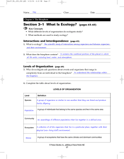
(e) Select a student at random and record the time spent studying statistics in the last
24-hour period:
S = 5any time t between 0 hours and 24 hours 1inclusive26 or S = [0, 24].
(f) Select a bus commuter at random and record the waiting time between his or her arrival
at a bus stop and the arrival of the next bus to that stop:
S = 5
L
7.5
t!
et's Do I
Voting Preference
Consider the process of randomly selecting two adults from Washtenaw County and recording
the voting preference for each adult as Republican, Democrat, Independent, or Other. The
two adults randomly chosen (in the order selected) are Ryan and Caitlyn. Which of the
following gives the correct sample space for the set of possible outcomes of this experiment?
Circle your answer.
(a)
(b)
(c)
(d)
S = 5Ryan, Caitlyn6.
S = 5Republican, Democrat, Independent, Other6.
S = 5Republican, Independent6.
None of the above.
ALIAMC07_0131497561.QXD 03/28/2005 05:55 PM Page 423
7.4 THE LANGUAGE OF PROBABILITY
423
Did you select (b) in the preceding “Let’s do it!” exercise? If so, you selected the correct
sample space if the random process had been to randomly select exactly one adult from
Washtenaw County and record his or her voting preference.
Did you select (c)? If so, you selected a set that represents just one of the possible individual outcomes, (R, I), which represents “Ryan is Republican and Caitlyn is Independent.” The correct answer is (d), since the actual sample space contains a total of 16 possible
individual outcomes. We should also note that the outcome (R, I) is different from the
outcome (I, R), which represents “Ryan is Independent and Caitlyn is Republican.” In other
words, the order of the responses does matter. If we actually surveyed a larger number of
adults and we were interested in learning about the proportion of adults for each of the
political preference categories, we might not be concerned about the order of the responses.
Subsets of the sample space are called events and are typically denoted by capital letters
at the beginning of the alphabet (A, B, C, and so on). In some cases, the sample space and
events may be represented using a Venn diagram.The sample space is represented by the box
and the events are a subset of the box.
A
a
S
b
Suppose that the outcome of the random process is a. Since outcome a is in the event A,
we say that the event A has occurred. If the outcome is b, since b is not in the event A, we say
that the event A has not occurred. If the random experiment were rolling a fair die, then the
sample space is given by S = 51, 2, 3, 4, 5, 66. Let the event A be defined as an odd outcome.
Then, the event A = 51, 3, 56 is a subset of S. If the die is rolled and a 1 is obtained, the event
A has occurred. If the die is rolled and a 2 is obtained, the event A has not occurred.
DEFINITION: An event is any subset of the sample space S. An event A is said to occur if
any one of the outcomes in A occurs when the random process is performed once.
L
7.6
t!
et's Do I
Expressing Events
Consider the experiment of rolling two fair dice. Circle the outcomes that correspond to the
following events:
(a) Event A = “No sixes.”
S = 5 11, 12
12, 12
13, 12
14, 12
15, 12
16, 12
11, 22
12, 22
13, 22
14, 22
15, 22
16, 22
11, 32
12, 32
13, 32
14, 32
15, 32
16, 32
11, 42
12, 42
13, 42
14, 42
15, 42
16, 42
11, 52
12, 52
13, 52
14, 52
15, 52
16, 52
11, 62
12, 62
13, 62
14, 62
15, 62
16, 62 6
ALIAMC07_0131497561.QXD 03/28/2005 05:55 PM Page 424
424
CHAPTER 7
HOW TO MEASURE UNCERTAINTY WITH PROBABILITY
(b) Event B = “Exactly one six.”
S = 5 11, 12
12, 12
13, 12
14, 12
15, 12
16, 12
11, 22
12, 22
13, 22
14, 22
15, 22
16, 22
11, 32
12, 32
13, 32
14, 32
15, 32
16, 32
11, 42
12, 42
13, 42
14, 42
15, 42
16, 42
11, 52
12, 52
13, 52
14, 52
15, 52
16, 52
11, 62
12, 62
13, 62
14, 62
15, 62
16, 62 6
11, 32
12, 32
13, 32
14, 32
15, 32
16, 32
11, 42
12, 42
13, 42
14, 42
15, 42
16, 42
11, 52
12, 52
13, 52
14, 52
15, 52
16, 52
11, 62
12, 62
13, 62
14, 62
15, 62
16, 62 6
11, 32
12, 32
13, 32
14, 32
15, 32
16, 32
11, 42
12, 42
13, 42
14, 42
15, 42
16, 42
11, 52
12, 52
13, 52
14, 52
15, 52
16, 52
11, 62
12, 62
13, 62
14, 62
15, 62
16, 62 6
(c) Event C = “Exactly two sixes.”
S = 5 11, 12
12, 12
13, 12
14, 12
15, 12
16, 12
11, 22
12, 22
13, 22
14, 22
15, 22
16, 22
(d) Event D = “At least one six.”
S = 5 11, 12
12, 12
13, 12
14, 12
15, 12
16, 12
11, 22
12, 22
13, 22
14, 22
15, 22
16, 22
L
7.7
t!
et's Do I
Favor or Oppose
In a group of people, some favor abortion (F) and others oppose abortion (O). Three people
are selected at random from this group, and their opinions in favor or against abortion are
noted. Assume that it is important to know which opinion came from each individual (that
is, that order does matter).
(a) Write down the sample space for this situation.
S =
(b) Write out the outcomes that make up the event A = “at most one person is against
abortion.”
A =
(c) Write out the outcomes that make up the event B = “exactly two people are in favor
of abortion.”
B =
ALIAMC07_0131497561.QXD 03/28/2005 05:55 PM Page 425
7.4 THE LANGUAGE OF PROBABILITY
Sometimes we are interested in events that are not so
simple. The event may be a combination of various
events. The union of two events is represented by A or
B, written mathematically as A ВЄ B and shown by the
shaded region in Figure 7.1. The union A or B contains
the outcomes that are in the event A or in the event B
or in both A and B. Sometimes the event of A or B is
stated as at least one of the two events has occurred.
Figure 7.1 Union
The intersection of two events is represented by A and
B, written mathematically as A Вє B and shown by the
shaded region in Figure 7.2. The intersection A and B is
comprised of only those outcomes that are in both the
event A and the event B. Often the word both is used
when describing the intersection of two events.
Figure 7.2 Intersection
425
A or B
A
S
B
Both A and B
A
S
B
The complement of an event is represented by not A,
written mathematically as AC and shown by the shaded
region in Figure 7.3. The complement of the event A is
comprised of all outcomes that are not in the event A. If
listing the outcomes that make up an event A seems a bit
overwhelming, it may be easier to summarize the outcomes that make up the complement of the event A.
Given the sample space S, every event A has a unique
complementary event AC in S.
Figure 7.3 Complement
Two events A and B are said to be disjoint if they have
no outcomes in common. Sometimes, instead of disjoint,
the events are said to be mutually exclusive. In terms of
mathematical notation, we would write A ВЁ B = В¤,
where ВЁ represents intersection, and В¤ represents the
empty set (the set that contains no outcomes). Two
events are disjoint if they cannot occur at the same time.
Disjoint events can be shown using a Venn diagram.
Figure 7.4 shows two events, A and B, that are disjoint.
Figure 7.4 Disjoint
AC
S
A
A
S
B
DEFINITION: Two events A and B are disjoint or mutually exclusive if they have no outcomes in common. Thus, if one of the events occurs, the other cannot occur.
The notion of mutually exclusive events can be extended to more than two events. For example, we say that the events A, B, and C are mutually exclusive if the events A and B have
no outcomes in common, the events A and C have no outcomes in common, and the events
B and C have no outcomes in common. Note that these conditions imply that the intersection of all three events, “A and B and C,” will also be empty.
ALIAMC07_0131497561.QXD 03/28/2005 05:55 PM Page 426
426
CHAPTER 7
HOW TO MEASURE UNCERTAINTY WITH PROBABILITY
Example 7.2
в—†
Disjoint Events
Problem
A random sample of 200 adults is classified according to their gender (male or female), and
highest education level attained (elementary, secondary, or college). The following table
summarizes the results.
Education
Gender
Male
Female
Elementary
Secondary
College
38
45
28
50
22
17
Consider the following events:
A = “adult selected has a college level education.”
B = “adult selected is a male with the highest level of education being secondary.”
C = “adult selected is a female.”
(a) Are the events A and B disjoint? Explain.
(b) Are the events A and C disjoint? Explain.
(c) Are the two row categories, “Male” and “Female,” disjoint events?
Solution
(a) Since no adult can have as the highest level of education attained both “secondary” and
“college,” the events A and B are disjoint.
(b) From the table we can see that an adult can be both a female and have college as the
highest level of education attained; in fact, there were 17 such adults. Hence, the events
A and C are not disjoint.
(c) Since an adult cannot be both male and female the row categories, male and female are
disjoint.The three column categories—elementary, secondary, and college—are the various levels for highest level of education attained and are also disjoint.
What We’ve Learned: The definition of mutually exclusive (or disjoint) events is a set
property. We simply determine if there are any items, in this case, people, that have both
attributes (corresponding to the two events in question).
L
7.8
t!
et's Do I
Mutually Exclusive?
For each scenario and list of events, determine whether the events are mutually exclusive:
(a) A retail sales agent makes a sale:
A = “the sale exceeds $50.”
B = “the sale exceeds $500.”
ALIAMC07_0131497561.QXD 03/28/2005 05:55 PM Page 427
7.4 THE LANGUAGE OF PROBABILITY
427
(b) A retail sales agent makes a sale:
A = “the sale is less than $50.”
B = “the sale is between $100 and $500.”
C = “the sale exceeds $1000.”
(c) Ten students are selected at random:
A = “no more than three are female.”
B = “at least seven are female.”
C = “at most five are female.”
7.4 EXERCISES
7.10
Each day a bus travels from City A to City D by way of Cities B and C (as shown). AndrГ© is
a traveler who can get on the bus at any one of the cities and can get off at any other city
along the route (except not the same city in which he got on the bus).
City A
City B
City C
City D
(a) Give the sample space (all possible outcome pairs) for representing the starting and ending points of André’s journey.
(b) Let E be the event that AndrГ© gets off at a city that comes after City B on the route of
the bus. List the outcomes from the sample space in part (a) that make up the event E.
7.11
Two chess players, Gabe and Ellie, decide to play several games of chess. They will stop playing if Gabe wins two matches or if they have played a total of three games in all. Each game
can be won by either Gabe or Ellie, and there can be no ties.
(a) Give the sample space (all possible outcomes) for the series of games played by Gabe
and Ellie.
(b) Let A be the event that no player wins two consecutive games. List the outcomes from
the sample space in part (a) that make up the event A.
7.12
Replacement and Order A basket contains three balls, one green, one yellow, and one white.
Two balls will be selected from the basket. For example, the outcome “G,Y” represents that
the green ball was selected, followed by the yellow ball.
Write out the corresponding sample space if
(a) the sampling procedure was with replacement and order matters.
(b) the sampling procedure was with replacement and order doesn’t matter.
(c) the sampling procedure was without replacement and order matters.
(d) the sampling procedure was without replacement and order doesn’t matter.
7.13
A simple random sample of students will be selected from a student body, and college status,
classified as either full time or part time, will be recorded.
(a) Give the sample space if just one student will be selected at random.
(b) Give the sample space if four students will be selected at random.
(c) Give the sample space if 20 students will be selected at random and the outcome of
interest is the number of full-time students.
7.14
At a formal conference a meeting takes place where one faculty member from each of the
nine different colleges attends. Upon all faculty members arriving, each shakes hands with
ALIAMC07_0131497561.QXD 03/28/2005 05:55 PM Page 428
428
CHAPTER 7
HOW TO MEASURE UNCERTAINTY WITH PROBABILITY
each other. How many handshakes are there? How can you express the answer in general if
the meeting consists of one faculty from each of N colleges?
7.15
Disjoint? Consider the experiment of drawing a card from a standard deck. Let
A = “heart,” B = “king,” and C = “spade.”
(a) Are the events A and B disjoint? Explain.
(b) Are the events A and C disjoint? Explain.
(c) Are the events B and C disjoint? Explain.
7.16
A travel agency offers ten different brochures, arranged in piles for customers to select from.
One of the employees told a customer to take any selection of brochures they wish but not
to take more than one of each kind. Assuming that the customer takes at least one brochure,
how many different selections are possible?
7.4.2 Rules of Probabilities
We return to the idea of probability and relate it to events and the outcomes of a sample
space. To any event A, we assign a number P(A) called the probability of the event A. Recall that the probability of an event was defined as the relative frequency with which that event
would occur in the long run. When the sample space contains a finite number of possible
outcomes, we have another technique for assigning the probability of an event:
в– Assign a probability to each individual outcome, each being a number between 0 and
1, such that the sum of these individual probabilities is equal to 1.
в– The probability of any event is the sum of the probabilities of the outcomes that make
up that event.
If the outcomes in the sample space are equally likely to occur, the probability of an event A
is simply the proportion of outcomes in the sample space that make up the event A. Do not
automatically assume that the outcomes in the sample space are equally likely—it will depend
on the random process and the definition of the outcome that is being recorded. Our first exercise does involve equally likely outcomes. Soon we will learn some probability rules that
will help us determine the probabilities of outcomes that are not equally likely.
L
7.9
t!
et's Do I
Assigning Probabilities to Events
Consider the experiment of rolling two fair dice. Assume that the 36 points in the sample
space are equally likely. What are the probabilities of the following events?
(a) Event A = “No sixes.”
S = 5 11, 12
12, 12
13, 12
14, 12
15, 12
16, 12
11, 22
12, 22
13, 22
14, 22
15, 22
16, 22
11, 32
12, 32
13, 32
14, 32
15, 32
16, 32
11, 42
12, 42
13, 42
14, 42
15, 42
16, 42
11, 52
12, 52
13, 52
14, 52
15, 52
16, 52
11, 62
12, 62
13, 62
14, 62
15, 62
16, 62 6
Since there are 25 of the 36 equally likely outcomes that comprise the event A, we have
P1A2 = 25
36 .
ALIAMC07_0131497561.QXD 03/28/2005 05:55 PM Page 429
7.4 THE LANGUAGE OF PROBABILITY
429
(b) Event B = “Exactly one six.”
P1B2 =
(c) Event C = “Exactly two sixes.”
P1C2 =
(d) Event D = “At least one six.”
P1D2 =
(e) Compare 1 - P1A2 with P(D). The events A and D are complementary events.
Basic Rules that Any Assignment of Probabilities Must Satisfy
1. Any probability is always a numerical value between 0 and 1.The probability is 0 if the
event cannot occur.The probability is 1 if the event is a sure thing—it occurs every time;
0 … P1A2 … 1.
2. If we add up the probabilities of each of the individual outcomes in the sample space,
the total probability must equal one; P1S2 = 1.
3. The probability that an event occurs is 1 minus the probability that the event does not
occur; P1A2 = 1 - P1AC2.
The third rule is called the complement rule. Any event and its corresponding complement are disjoint sets, which when brought back together give us the whole sample space S.
The probability of the sample space S is 1, so the probabilities of the event and its complement must add up to 1.This rule can be very useful. If finding the probability of an event seems
too difficult, see if finding the probability of the complement of the event is easier.
Think About It
Consider the experiment of tossing a fair coin 10 times.Think about what is the sample space
S. Let A be the event of “at least 1 head.” At least 1 head means exactly 1 head or exactly
2 heads or exactly 3 heads or exactly 4 heads or exactly 5 heads or exactly 6 heads or exactly
7 heads or exactly 8 heads or exactly 9 heads or all 10 heads. That is a lot of outcomes to
try to count up. Think about what is the complement of A, and then find the probability of
the event A using the complement rule.
ALIAMC07_0131497561.QXD 03/28/2005 05:55 PM Page 430
430
CHAPTER 7
HOW TO MEASURE UNCERTAINTY WITH PROBABILITY
L
7.10
t!
et's Do I
A Fair Die?
A die, with faces 1, 2, 3, 4, 5, 6, is suspected to be unfair in the sense of having a tendency
toward showing the larger faces. We wish to test the following hypotheses:
H0: The die is fair (that is, it has an equal chance for all six faces).
H1: The die has a tendency toward showing larger faces.
For the data, you will roll the die two times. Recall the 36 possible pairs of faces if you roll a
die two times:
S = 5 11, 12
12, 12
13, 12
14, 12
15, 12
16, 12
11, 22
12, 22
13, 22
14, 22
15, 22
16, 22
11, 32
12, 32
13, 32
14, 32
15, 32
16, 32
11, 42
12, 42
13, 42
14, 42
15, 42
16, 42
11, 52
12, 52
13, 52
14, 52
15, 52
16, 52
11, 62
12, 62
13, 62
14, 62
15, 62
16, 62 6.
The sum of the two rolls will be the response used to make the decision between the two
hypotheses.
(a) Consider the possible sum of 11. Circle the outcomes in the accompanying sample space
that correspond to having a sum of 11. What is the probability of getting a sum of 11 on
the next two rolls?
The suggested format for the decision rule is to reject H0 if the sum of the two rolls is too large.
(b) The direction of extreme is (circle one)
one-sided to the right.
one-sided to the left.
two-sided.
(c) What is the p-value if the observed sum actually equals 11? (Hint: Think about the
definition of a p-value.)
(d) Would an observed sum of 11 be statistically significant at the 5% significance level? at
the 10% level? Explain.
Our next basic rule tells us how to find the probability of
the union of two events—that is, the probability that one
or the other event occurs. The basis of this rule is easy to
see by looking at the corresponding diagram. We start
by taking those outcomes in the event A, and then add all
of those outcomes that form the event B. The outcomes
that occur in both A and B have been included twice, so
we need to subtract them once.
A or B
A
S
B
ALIAMC07_0131497561.QXD 03/28/2005 05:55 PM Page 431
7.4 THE LANGUAGE OF PROBABILITY
431
The Addition Rule
4. The probability that either the event A or the event B occurs is the sum of their
individual probabilities minus the probability of their intersection.
P1A or B2 = P1A2 + P1B2 - P1A and B2
If the two events A and B do not have any outcomes in common (that is, they are
disjoint), then the probability that one or the other occurs is simply the sum of their
individual probabilities.
If A and B are disjoint events, then P1A or B2 = P1A2 + P1B2.
Note: This special case can be extended to more than two disjoint events. If the events
A, B, and C are disjoint, then P1A or B or C2 = P1A2 + P1B2 + P1C2.
Example 7.3
в—†
Gender versus Education
Problem
Recall the data from Example 7.2 based on a random sample of 200 adults classified by gender and by highest education level attained.
Education
Gender
Elementary
Secondary
College
38
45
28
50
22
17
88
112
83
78
39
200
Male
Female
Consider the following two events:
A = “adult selected has a college-level education.”
C = “adult selected is a female.”
What is the probability that an adult selected at random either has a college level of
education or is a female?
Solution
P1A or C2 = P1A2 + P1C2 - P1A and C2
=
39
200
+
112
200
-
17
200
=
134
200
= 0.67
What We’ve Learned: In general, when the two events are not disjoint, P1A or B2 Z
P1A2 + P1B2.
ALIAMC07_0131497561.QXD 03/28/2005 05:55 PM Page 432
432
CHAPTER 7
HOW TO MEASURE UNCERTAINTY WITH PROBABILITY
L
7.11
t!
et's Do I
Winning Contracts
A local construction company has entered a bid for two contracts for the city. The company
feels that the probability of winning the first contract is 0.5, the probability of winning the
second contract is 0.4, and the probability of winning both contracts is 0.2.
(a) What is the probability that the company will win at least one of the two contracts (that
is, the probability of winning the first contract or the second contract)?
(b) The corresponding Venn diagram displays the events A = “win first contract” and
B = “win second contract.” Two of the probabilities have been entered. Note that the 0.2 and the
0.3 sum to the probability for the event A of 0.5.
Add the remaining probabilities such that the total
B
0.2
of all of the probabilities is equal to 1.
S
A
0.3
(c) What is the probability of winning the first contract
but not the second contract? (Hint: Look at the
portion of the diagram that represents the event of
interest.)
(d) What is the probability of winning the second contract but not the first contract?
(Hint: Look at the portion of the diagram that represents the event of interest.)
(e) What is the probability of winning neither contract?
(Hint: Look at the portion of the diagram that represents the event of interest.)
Sometimes, we will have some given information about the outcome of the random
process. We may wish to update the probability of a certain event occurring taking into account this given information. Consider rolling a single fair die one time. The sample space is
S = 51, 2, 3, 4, 5, 66, and each of the six outcomes is equally likely.The probability of getting
the value of 1 is then 16. But suppose that we know the outcome was an odd value: Now, what
is the probability that the value is a 1? Since we know the outcome was an odd value, we no
longer consider the original sample space as the set of possible outcomes. There are only
three possible outcomes in the updated sample space—namely, 51, 3, 56. Each of these three
outcomes is now equally likely.Thus, the updated probability is 13. What we have just computed
is a conditional probability, the probability of the event A = 516, given the event
B = 5ODD6 has occurred, represented by the general expression P1AЖ’B2. In other words,
conditioning on the fact that the event B has occurred, we wish to find the updated probability that the event A will occur.
Our next rule tells us how to find such A given B
Original sample
space S
conditional probabilities. The basis of this
B П­ updated sample space
rule is easy to see by looking at the corresponding diagram. Since we know that the
A
event B has occurred, we start by taking only
those outcomes in the event B. This set of
B
outcomes is our updated sample space and
will form the base of our probability expression. We wish to find the probability of the
ALIAMC07_0131497561.QXD 03/28/2005 05:55 PM Page 433
7.4 THE LANGUAGE OF PROBABILITY
433
event A occurring on this updated sample space. The only outcomes in the event A included in this updated sample space are those belonging to both the event A and the event B (that
is, the outcomes that comprise the intersection between A and B).
Conditional Probability
5. The conditional probability of the event A occurring, given that event B has occurred,
is given by
P1A and B2
, if P1B2 7 0.
P1AЖ’B2 =
P1B2
Note: We could rewrite this rule and have an expression for calculating an intersection,
called the multiplication rule.
P1both events will occur at the same time2
= P1A and B2 = P1B2P1AЖ’B2 = P1A2P1BЖ’A2
The basis of this rule is as follows: For both events to occur, first we must have one occur (for
example, the event B), and then given that B has occurred, the event A must also occur.
Of course, the events A and B could be switched around, which gives us the last part of the
preceding result.
Example 7.4
в—†
Gender versus Education
Problem
Recall the data from Example 7.2 based on a random sample of 200 adults classified by gender and by highest education level attained.
Education
Gender
Elementary
Secondary
College
38
45
28
50
22
17
88
112
83
78
39
200
Male
Female
Consider the following two events:
A = “adult selected has a college-level education.”
C = “adult selected is a female.”
What is the probability that an adult selected at random has a college level of education
given that the adult is a female? That is, find P1AЖ’C2.
Solution
Since we are given that the selected adult is a female, we only need to consider the 112
females as our updated sample space. Among the 112 females, there were 17 females who
had a college level education.
17
P1AЖ’C2 = P1college level education Ж’female2 =
= 0.152
112
If we use the more formal rule, we have:
P1AЖ’C2 =
P1A and C2
=
P1C2
17
200
112
200
=
17
= 0.152.
112
ALIAMC07_0131497561.QXD 03/28/2005 05:56 PM Page 434
434
CHAPTER 7
HOW TO MEASURE UNCERTAINTY WITH PROBABILITY
What We’ve Learned: If the information about the events is presented in a two-way frequency table of counts, finding conditional probabilities is straightforward. In this example,
the given event was “female,” so we focused only on the female row of counts and expressed
the number with a college-level education as a fraction of the total number of females.
L
7.12
t!
et's Do I
Union Proposal
Before contract discussions, the state-wide union made a proposal that emphasizes fringe
benefits rather than wage increases.The opinions of a random sample of 2500 union members
are summarized in the following table:
Opinion
Gender
Female
Male
Favor
Neutral
Opposed
800
400
200
100
500
500
(a) Complete the table by computing the row and column totals.
(b) What is the probability that a randomly selected union member will be opposed?
P1opposed2 =
(c) What is the probability that a randomly selected female union member will be opposed?
Note that you are given that the selected union member is a female so you can focus on
only the female union members and determine what proportion of them are opposed.
P1opposed Ж’female2 =
(d) Give an example of two events represented in the above table that are mutually exclusive (i.e., they are disjoint).
L
7.13
t!
et's Do I
Computing a Conditional Probability
Suppose two fair dice are rolled. Given that the faces show different numbers, what is the
probability that one face is a 4?
ALIAMC07_0131497561.QXD 03/28/2005 05:56 PM Page 435
7.4 THE LANGUAGE OF PROBABILITY
435
L
7.14
t!
et's Do I
More Conditional Probabilities
Scenario I The random process is rolling a fair die one time.
The sample space is S = 51, 2, 3, 4, 5, 66.
P122 =
(a) What is the probability of getting a 2?
P12 Ж’Even2 =
(b) Suppose that we know that the outcome was
an even value; now, what is the probability of
getting a 2?
Scenario II The random process is tossing a fair coin two times.
The sample space is S = 5HH, HT, TH, TT6.
P1H on 2nd2 =
(a) What is the probability of getting a head on the
second toss?
(b) What is the probability of getting a head on the
P1H on 2nd Ж’H on 1st2 =
second toss, given it was a head on the first toss?
Think About It
In Scenario I of the preceding exercise, how do your answers to parts (a) and (b) compare?
In Scenario II, how do your answers to parts (a) and (b) compare?
What makes these two scenarios different?
Suppose that for events A and B we have P1AЖ’B2 = 0.3 and P1A2 = 0.3. What does this tell
us about the two events A and B? This is what happened in Scenario II of the previous exercise. If knowing that event B occurred does not change the probability of the event A
occurring—that is, P1AƒB2 = P1A2—we say the two events are independent.
DEFINITION: Two events A and B are independent if P1AЖ’B2 = P1A2 or, equivalently, if
P1BЖ’A2 = P1B2.
If two events do not influence each other (that is, if knowing one has occurred does not
change the probability of the other occurring), the events are independent. If two events
are independent, the multiplication rule tells us that the probability of them both occurring together is found by multiplying their individual probabilities:
If two events A and B are independent (only in this case), then P1A and B2 = P1A2P1B2.
ALIAMC07_0131497561.QXD 03/28/2005 05:56 PM Page 436
436
CHAPTER 7
HOW TO MEASURE UNCERTAINTY WITH PROBABILITY
Example 7.5
в—†
Gender versus Education
Problem
Recall the data from Example 7.2 based on a random sample of 200 adults classified by
gender and by highest education level attained.
Education
Gender
Elementary
Secondary
College
38
45
28
50
22
17
88
112
83
78
39
200
Male
Female
Consider the following two events:
A = “adult selected has a college level education.”
C = “adult selected is a female.”
Are these two events A and C independent?
Solution
From Examples 7.3 and 7.4, we have the following probabilities:
39
= 0.195
P1A2 = P1adult selected has a college level education2 = 200
P1AЖ’C2 = P1adult selected has a college level education given the adult is a female2
17
=
= 0.152.
112
Since knowing the adult is a female changes the probability that the adult will have a collegelevel education (from 0.195 to 0.152), these two events A and C are not independent.
Alternatively, we could have checked for the independence of the two events using the
multiplication rule for independent events. Is P(A and C) equal to P(A) P(C)? We have
P1A and C2 = P1adult selected has a college level education and is a female2
17
= 0.085 and
200
39
112
P1A2P1C2 = a
ba
b = 0.109.
200 200
=
Since P1A and C2 Z P1A2P1C2, we can conclude that these two events are not independent.
What We’ve Learned: We do not have to show both rules for assessing independence; just
one is sufficient and will imply the same conclusion as the other rule.To determine which rule
you might use for a particular problem, take a look at the probabilities that you may have
already computed.
Example 7.6
Problem
Gerald Kushel, Ed.D., is the author of several books, including Effective Thinking for
Uncommon Success. In a 1991 interview for Bottom Line Personal newsletter, Dr. Kushel
reported the results of a survey conducted to study success. A total of 1200 people were
ALIAMC07_0131497561.QXD 03/28/2005 05:56 PM Page 437
7.4 THE LANGUAGE OF PROBABILITY
437
questioned, among whom were lawyers, artists, teachers, and students. He found that 15%
enjoy neither their jobs nor their personal lives, 80% enjoy their jobs but not their personal
lives, and 4% enjoy both their jobs and their personal lives.
(a) Complete the Venn diagram below. Provide all probabilities in the blank rectangles.
P П­ Enjoy
Personal
Life
J П­ Enjoy Job
(b) How many people interviewed said they enjoy their personal lives but not their jobs?
(c) Given a person enjoys their job, what is the probability they enjoy their personal life?
(d) Are the events enjoy their job and enjoy their personal life mutually exclusive?
Explain.
(e) Are the events enjoy their job and enjoy their personal life independent? Explain.
Solution
(a) The completed Venn diagram is shown below.
P П­ Enjoy
Personal
Life
J П­ Enjoy Job
0.01
0.04
0.80
0.15
(b) Twelve people, since 0.01 * 1200 = 12.
(c) P1Enjoy personal life Ж’Enjoy job2 = 0.04
0.84 = 0.048.
(d) No. They are not mutually exclusive (or disjoint) events because there are 48 people
who enjoy both their job and their personal life.
(e) Since P1Enjoy personal life Ж’Enjoy job2 = 0.048 is not equal to P1Enjoy personal life2 =
0.05, these two events are not independent.
What We’ve Learned: The Venn diagram can provide a nice way to picture the different
events and express probabilities of the various parts. When writing in probabilities, it is generally easiest to start with the value in the intersection of the events. Then determine the values for each part that does not include the intersection.
ALIAMC07_0131497561.QXD 03/28/2005 05:56 PM Page 438
438
CHAPTER 7
HOW TO MEASURE UNCERTAINTY WITH PROBABILITY
L
7.15
t!
et's Do I
A Family Plan Revisited
Recall from “Let’s do it! 7.1” that we discussed a couple that planned to have children until
they have a boy or until they have three children, whichever comes first.Through simulation,
we estimated the probability that they will have a boy among their children. What was your
estimate?
We now have the probability background to be able to find the actual probability of
0.875. We assumed that
1. each child has probability 1Нћ2 of being a boy and 1Нћ2 of being a girl;
2. the gender of successive children is independent, that is, knowing the gender of a child
does not influence the gender of any of the successive children.
First, we need to generate the sample space.Three of
Probability
the four possible outcomes are listed in the accompanying
1
B
diagram.These three outcomes result in the couple having
2
a boy. Fill in the one remaining possible outcome. Next,
1 1
( ) 1
GB
2 2 П­ 4
we compute the probability for each of the outcomes,
SП­
1 1
using the preceding assumptions. Some of the probGGB
( )( 12 )П­ 18
2 2
abilities have been computed for you. Find the remaining
probabilities and verify that they add up to 1.
———
To find the probability that they will have a boy
among their children, we need to add up the probabilities
of the events that correspond to having a boy—namely, the probabilities for the first three
outcomes in the sample space.
.
P1having a boy among their children2 =
Convert your answer to decimal form, and you should have 0.875 as the probability.
L
7.16
t!
et's Do I
Getting Good Business?
The GOOD (not Better) Business Bureau conducts a survey of the quality of service offered
by the 86 auto repair shops in a certain city. The results on Service and Shop Type are
summarized in the following table:
Service
Shop Type
New-Car Dealership
Individual Shop
Good
Questionable
18
34
6
28
(a) What is the probability that a randomly selected shop provides good service?
(b) What is the probability that a randomly selected shop is an individual shop?
ALIAMC07_0131497561.QXD 03/28/2005 05:56 PM Page 439
7.4 THE LANGUAGE OF PROBABILITY
439
(c) What is the probability that a randomly selected shop is an individual shop and provides good service?
(d) What is the probability that a randomly selected individual shop provides good service?
(e) Are the events “individual shop” and “provides good service” mutually exclusive? Explain.
(f) Are the events “individual shop” and “provides good service” independent? Explain.
Think About It
Consider the random process of tossing a fair coin six times.
1. Which of the following sequences of tosses is more likely to occur?
(a) THTHHT
(b) HHHTTT
(c) HHHHHH
Check your answer by finding the probability of each of the sequences.
Hint: Remember that successive tosses of a coin are assumed to be independent.
2. If we observe HHHHHH, is the next toss more likely to give a tail than a head?
Hint: Think about whether or not the coin has any memory about the first six tosses.
Mutually Exclusive and Independent Events
Initially, it can be easy to confuse the two definitions of mutually exclusive events and
independent events. It is important to keep the two definitions separate.
в– в– The definition of mutually exclusive events is based on a set property. You can easily
visualize mutually exclusive events by using a Venn diagram (the two sets do not overlap). So if two events are mutually exclusive and you are given that one of the events
has occurred, the probability that the other event will occur is 0.
The definition of independent events is based on a probability property. You cannot
easily visualize independent events by using a Venn diagram, which must include probabilities that relate in a certain way. If two events are independent and you are given
that one of the events has occurred, the probability that the other event will occur is
not changed.
For Mutually Exclusive Events
For Independent Events
P1A and B2 = 0
P1A and B2 = P1A2P1B2
P1A or B2 = P1A2 + P1B2
P1A or B2 = P1A2 + P1B2 - P1A2P1B2
P1AЖ’B2 = 0
P1AЖ’B2 = P1A2
ALIAMC07_0131497561.QXD 03/28/2005 05:56 PM Page 440
440
CHAPTER 7
HOW TO MEASURE UNCERTAINTY WITH PROBABILITY
7.4 EXERCISES
7.17
What Is the Error? Identify the error, if any, in each statement. If no error, write “no error.”
(a) The probabilities that an automobile salesperson will sell 0, 1, 2, or at least 3 cars on a
given day in February are 0.19, 0.38, 0.29, and 0.15, respectively.
(b) The probability that it will rain tomorrow is 0.40 and the probability that it will not rain
tomorrow is 0.52.
(c) The probabilities that the printer will make 0, 1, 2, 3, or at least 4 mistakes in printing a
document are 0.19, 0.34, -0.25, 0.43, and 0.29, respectively.
(d) On a single draw from a deck of playing cards, the probability of selecting a heart is 14, the
probability of selecting a black card (i.e., spade or club) is 12, and the probability of
selecting both a heart and a black card is 18.
7.18
Students in a certain class were asked whether they had eaten at various local restaurants.
Two of the Mexican restaurants on the questionnaire were Arriba and Bandido. The results
were used to obtain the following probabilities:
The probability that a randomly selected student has eaten at Arriba is 0.30.
The probability that a randomly selected student has eaten at Bandido is 0.40.
The probability that a randomly selected student has eaten at Arriba, but not Bandido,
is 0.20.
(a) Complete the following Venn diagram by filling in each empty box with the probability
for the section that the box is in:
Arriba
Bandido
(b) What is the probability that a student selected at random will have eaten at both Arriba
and at Bandido?
(c) What is the probability that a student selected at random will have not eaten at Arriba
nor at Bandido?
7.19
Three teams, the Lions, the Tigers, and the Panthers, will play each other in a soccer tournament. The following probabilities are given about the upcoming games:
The probability that the Lions will beat the Tigers is 0.40.
The probability that the Lions will beat the Tigers and the Panthers is 0.20.
The probability that the Panthers will beat the Lions is 0.30.
(a) What is the probability that the Lions will beat the Panthers?
(b) Complete the following Venn diagram by filling in each empty box with the probability
for the section that the box is in:
Lions beat
Tigers
Lions beat
Panthers
ALIAMC07_0131497561.QXD 03/28/2005 05:56 PM Page 441
7.4 THE LANGUAGE OF PROBABILITY
441
(c) What is the probability that the Lions will win at least one of the matches against the
Tigers and the Panthers?
(d) Given that the Lions beat the Tigers, what is the probability that the Lions will beat the
Panthers?
7.20
A study was conducted to assess the effectiveness of a new medication for seasickness as
compared to a standard medication. A group of 160 seasick patients were randomly divided
into two groups, with the first 80 selected at random assigned to receive the new medication
and the other 80 assigned to the receive the standard medication. The results are presented
in the following table:
Medication
Response
Improved
Did Not Improve
New
Standard
60
20
48
32
(a) What is the probability that a randomly selected patient will improve?
(b) Given that the patient received the standard medication, what is the probability that the
patient will improve?
(c) Given that the patient received the new medication, what is the probability that the
patient will improve?
(d) The first 80 randomly selected patients were assigned to the new medication. Using your
calculator (with a seed value of 58) or the random number table (Row 24, Column 1), give
the labels for the first five patients to receive the new medication.
7.21
Consider the following set of short probability questions. Use the rules and results from this
chapter to answer each question.
(a) If the probability of buying a pair of shoes is 0.52 and the probability of buying a dress
is 0.67, and these two events are independent, find the probability of buying an outfit; that
is, a pair of shoes and a dress.
(b) You bought two turtledoves not knowing their sex.If the probability of getting a female turtledove is 0.59, find the probability of getting at least one female turtledove in the pair you
bought.Assume the sex of one turtledove is independent of the sex of the other turtledove.
(c) Three foreign students are applying to medical school. If the probability that one student
has a French citizenship is 0.78, find the probability that exactly two of these students will
have French citizenship. Assume that the citizenship of a student is independent of that
for another student.
(d) Suppose you have four friends.You would like to call and invite the first one, who accepts
your invitation to go to the movies with you. If the probability that a friend actually
accepts the invitation is 0.75, find the probability that the first friend to accept the
invitation occurs on your third attempt.
(e) You found five golden earrings on a beach. If the probability of finding a real golden
earring on a beach is 0.43, find the probability of getting three or fewer real golden
earrings among the five.
(f) In an amusement park you decide to play a game where if you shoot inside a circle you
win a prize. If the probability of getting a prize is 0.38, find the probability of getting a
prize on or before the fourth trial. Assume that the trials are independent.
7.22
The results of a study relating physical attractiveness to helping behavior are shown here:
Physical Attractiveness
Helping
Behavior
Helped (H)
Did not Help (NH)
Attractive (A)
Unattractive (NA)
34
46
26
54
ALIAMC07_0131497561.QXD 03/28/2005 05:56 PM Page 442
442
CHAPTER 7
HOW TO MEASURE UNCERTAINTY WITH PROBABILITY
(a) What is the probability of randomly selecting a subject who helped?
(b) Given that the person was attractive, what is the probability the subject helped?
(c) Given that the person was not attractive, what is the probability the subject helped?
7.23
The question of whether or not birth order is related to juvenile delinquency was examined
in a large-scale study using a high school population. A total of 1160 girls attending the public high school were given a questionnaire that measured the degree to which each had exhibited delinquent behavior. Based on the answers to the questions, each girl was classified as
either delinquent or not delinquent. The results are summarized in the following table:
Birth Order
Delinquency
Status
Oldest
In Between
Youngest
Only Child
TOTAL
Yes
20
30
35
25
110
No
450
310
215
75
1050
TOTAL
470
340
250
100
1160
(a) Calculate the probability that a high school girl selected at random from those surveyed
will be delinquent.
(b) Calculate the probability that a high school girl selected at random from those surveyed
will be delinquent given that they are the oldest child.
(c) Are the events “oldest child” and “delinquent” independent? Give support for your
answer.
7.24
A survey of automobile ownership was conducted for 200 families in Houston, Texas. The
results of the study showing ownership of automobiles of United States and foreign manufacturers are summarized as follows:
Do you own a U.S. car?
Do you own a foreign car?
Yes
No
Yes
No
30
150
10
10
(a) What is the probability that a randomly selected family will own a U.S. car and foreign
car?
(b) What is the probability that a randomly selected family will not own a U.S. car?
(c) Given that a randomly selected family owns a U.S. car, what is the probability that they
will also own a foreign car?
(d) Are the events “own a U.S. car” and “own a foreign car” independent events? Give
support for your answer.
7.25
In an experiment to study the dependence of hypertension on smoking habits, the following
data were collected on 180 individuals:
Smoking Status
Hypertension
Status
Nonsmoker
Moderate smoker
Heavy smoker
Hypertension
21
36
30
No Hypertension
48
26
19
(a) What is the probability that a randomly selected individual is experiencing hypertension?
(b) Given that a heavy smoker is selected at random from this group, what is the probability
that the person is experiencing hypertension?
(c) Are the events “hypertension” and “heavy smoker” independent? Give supporting
calculations.
ALIAMC07_0131497561.QXD 03/28/2005 05:56 PM Page 443
7.4 THE LANGUAGE OF PROBABILITY
7.26
443
A random sample of 200 adults is classified according to gender and attained education level.
Education
Gender
Elementary
Secondary
College
Male
38
28
22
Female
45
50
17
If a person is picked at random from this group, what is the probability that
(a) the person is male, given that the person has a secondary education?
(b) the person does not have a college degree, given that the person is female?
(c) Are the events “male” and “secondary education” independent? Give supporting
calculations.
7.27
Based on the orders of many of its customers, a bagel-store manager has found that 30% of
the customers are male and 40% of the customers order coffee. We also have that the events
“male” and “order coffee” are independent.
(a) Complete the following Venn diagram by filling in each empty box with the probability
for the section that the box is in:
Coffee
Male
(b) What is the probability that a customer selected at random will be male and will not
order coffee?
7.28
An article entitled “Test Your Own Cholesterol” (Source: Ann Arbor News, March 8, 1995) describes
a home cholesterol test manufactured by Chem Trak. The article states that “Americans are
becoming more savvy about cholesterol, Á 65 percent of adults have had their total cholesterol measured.” Suppose that two American adults will be selected at random. Assume that
the responses from these two adults are independent. What is the probability that both will
have had their total cholesterol measured?
7.29
The utility company in a large metropolitan area finds that 82% of its customers pay a given
monthly bill in full. Suppose that two customers are chosen (at random) from the list of all customers. Assume that the responses from these two customers are independent. What is the
probability that at least one of the two customers will pay their next monthly phone bill in full?
7.30
Eighty percent of the residents of Washtenaw County are registered to vote. If four
Washtenaw County residents who are old enough to vote are selected at random, what is the
probability of obtaining no registered voters? (Assume that the responses of the four
selected residents are independent.)
7.31
In a community college, 40% of the students oppose funding of special-interest groups. If a
random sample of three students is selected and the opinions of these three students can be
assumed to be independent, what is the probability that none of the three oppose funding of
special-interest groups?
7.32
Suppose that you have invested in two different mutual funds. If the first mutual fund makes
money, the probability that the second one will also make money is 0.7. If the first mutual
fund loses money, the probability that the second one will make money is still 0.7. Given this
ALIAMC07_0131497561.QXD 03/28/2005 05:56 PM Page 444
444
CHAPTER 7
HOW TO MEASURE UNCERTAINTY WITH PROBABILITY
information, we would say that the two mutual funds would be considered as
Select one of the following:
(a) mutually exclusive events.
(b) dependent investments.
(c) independent investments.
(d) complementary events.
.
7.33
Suppose you have 12 blue socks and 18 brown socks scrambled in your drawer. What is the
minimum number of socks you have to pull out (in the dark) to have a matched pair with
certainty?
7.34
Consider two events, A and B, of a sample space such that P1A2 = P1B2 = 0.6.
(a) Is it possible that the two events A and B are mutually exclusive? Explain.
(b) If the events A and B are independent, what would be the probability that the two events
occur together—that is, the probability of P(A and B)?
(c) If the events A and B are independent, what would be the probability that at least one
of the two events will occur—that is, the probability of P(A or B)?
(d) Suppose that the probability of the event B occurring, given that event A has occurred,
is 0.5—that is, P1BƒA2 = 0.5. What is the probability that at least one of the two events
will occur—that is, the probability of P(A or B)?
7.35
Determine whether each of the following statements is true or false:
(a) Two events that are disjoint (mutually exclusive) are also always independent.
(b) Suppose that among all students taking a certain test 10% cheat. If two students are
selected at random (independently), the probability that both cheat is 0.01.
7.36
A Coin and a Die A random process consists of flipping a fair coin, and then flipping it
a second time if a head occurs on the first flip. If a tail occurs on the first flip, a fair die is
tossed once.
(a) Give the sample space for this random process.
(b) Let the events A and B be defined as follows:
A = “tail on first flip and 1 on die” = 5T16, and
B = “head on first flip and head of second flip” = 5HH6.
Find the probability of each of these events. (Hint: Use the multiplication rule.)
7.37
(a) If two events are mutually exclusive, are their complements also mutually exclusive?
Explain.
(b) If two events are independent, are their complements also independent? Explain.
7.4.3 Partitioning and Bayes’s Rule*
We wish to find the probability of the event A, but finding the probability is not always so straightforward.
Suppose that we have information about the likelihood
of the event A, not overall, but for two subgroups of
the sample space, say B1 and B2, which are shown in
the accompanying diagram. So we know P1AЖ’B12 and
P1AЖ’B22. We would like to combine the probabilities of
A for each piece to get the P1A2 overall. The two
events, B1 and B2, form a partition of the sample space.
In this case, the event B2 is actually the complement
of the event B1.
*The probability results in this section are optional.
B1
B2
S
A
ALIAMC07_0131497561.QXD 03/28/2005 05:56 PM Page 445
7.4 THE LANGUAGE OF PROBABILITY
445
DEFINITION: The events B1, B2, ГЃ BI form a partition of the sample space S if
1. the events B1, B2, ГЃ , BI are mutually exclusive and
2. the union of B1, B2, ГЃ , BI is the sample space S.
Note: The events form a partition if each individual outcome of the sample space lies in
exactly one of the events.
How can we find the overall probability of the event A? First, we consider the two disjoint
parts of event A: P1A2 = P1A and B12 + P1A and B22. Next, we apply the multiplication
rule for two events to each of the two probabilities on the righthand side.
P1A2 = P1AЖ’B12P1B12 + P1AЖ’B22P1B22
The two conditional probabilities of the event A, given that you are on a particular part of the
sample space, are pooled together by weighing each by the chance of being on the particular
part of the sample. This last line is called the partition rule or law of total probability.
Partition Rule
6. If the events B1 and B2 form a partition of S, then
P1A2 = P1AЖ’B12P1B12 + P1AЖ’B22P1B22.
This result can be extended to a partition of more than two events: If the events B1, B2, ГЃ ,
BI form a partition of S, then
P1A2 = P1AЖ’B12P1B12 + P1AЖ’B22P1B22 + ГЃ + P1AЖ’BI2P1BI2.
Example 7.7
в—†
Two-Stage Experiment
Problem
Suppose that there are two boxes of balls, as shown
in the picture. Consider the following two-stage
experiment:
Stage 1: Pick a box at random (that is, with equal
probability).
Stage 2: From that box, pick one ball at random.
Box I
(a) What is the chance of getting a teal ball from Box I?
(b) What is the chance of getting a teal ball from Box II?
(c) What would be the overall probability of getting a teal ball?
Solution
(a) P1tealЖ’BI2 = 24.
(b) P1tealЖ’BII2 =
4
10 .
Box II
ALIAMC07_0131497561.QXD 03/28/2005 05:56 PM Page 446
446
CHAPTER 7
HOW TO MEASURE UNCERTAINTY WITH PROBABILITY
(c) P1teal2 = P1tealЖ’BI2P1BI2 + P1tealЖ’BII2P1BII2
= 12421122 + 1104 21122
= 0.45.
What We’ve Learned: In this example, the calculation of the probability of getting a teal
ball obviously depends on which box is selected—the two boxes form what is called a partition. Since in Stage 1 of the experiment a box is selected at random, the probability that we
select any given box is 12. Finally, in part (c) we used the partition rule, a form of weighted
average, to combine the two probabilities from parts (a) and (b).
L
7.17
t!
et's Do I
Defective Razors
A store sells three different types of disposable razors. The probability that the type A razors
will be defective is 0.3, and the probability that Type B and C razors will be defective are 0.2
and 0.1, respectively. Suppose that 20% of the razors are of Type A, 30% are of Type B, and
the rest are of Type C.
What is the probability that a randomly selected razor will not be defective?
One interesting application of the partition rule is called the Warner’s randomized response
model, which is discussed in the next example. Suppose that we want to estimate the proportion of high school students in a school district who have engaged in illicit drug use.Asking
this question directly would probably yield little useful information. How can we get accurate answers to a sensitive question that respondents might be reluctant to answer truthfully?
Example 7.8
в—†
Getting Answers to Sensitive Questions
Problem
Set up a survey with two questions. Let Q1 be the sensitive question. Then, the second question, Q2, is any other question for which you know what proportion of “yes” responses you
should expect to get. For example,
Survey
Q1: “Have you ever shoplifted?”
Q2: “Is the second flip of your fair coin a head?”
YES
YES
NO
NO
ALIAMC07_0131497561.QXD 03/28/2005 05:56 PM Page 447
7.4 THE LANGUAGE OF PROBABILITY
447
The respondent determines which question he or she answers using some probability
device under his or her control. For example, we could have the respondent flip a fair coin
two times. If the first flip results in a 5H6, the respondent is to answer question Q1 truthfully, and if the flip results in a 5T6, the respondent is to answer question Q2 truthfully.
Since only the respondent knows which question he or she is answering, there should be no
stigma attached to a “yes” or “no” response. Although everyone flips the fair coin two times,
the result of the second flip would only be needed if the first flip was a 5T6. But can we still
find out the proportion who respond “yes” to the sensitive question?
We wish to learn about the proportion in the population for which the true response
to question Q1 is “yes”—that is, the probability of a yes response, given question Q1.
Applying the partition rule to the event “yes,” with the partition being Q1 or Q2, we have
P1YES2 = P1YES Ж’Q12P1Q12 + P1YES Ж’Q22P1Q22.
We would know, by the probability device used to determine which question is answered, the
values of P(Q1) and P(Q2). We would also know the value of P1YES Ж’Q22. For the second
flip of a fair coin question, it would be 0.50. We would use the proportion of “yes” responses
to estimate the P(YES). All that remains is the probability of interest, P1YES Ж’Q12, which
we can solve for.
If 41% of those surveyed responded with a “yes.” Calculate P1YESƒQ12 and interpret
what it means.
Solution
P1YES2 = P1YES Ж’Q12P1Q12 + P1YES Ж’Q22P1Q22
0.41 = P1YES Ж’Q1210.52 + 10.5210.52
0.41 - 10.5210.52
0.5
P1YES Ж’Q12 = 0.32
P1YES Ж’Q12 =
So we would estimate that about 32% of the population represented by this sample have
shoplifted.
What We’ve Learned: Probability can help us find answers to questions that would be
difficult to ask directly and get good answers. This particular method works better if the
number of those surveyed is large.
L
7.18
t!
et's Do I
Getting Answers to Sensitive Questions
Perform the Warner’s randomized response model with the students in your class.
в– в– Determine the sensitive question of interest and enter it in the survey below as Q1.
Select two random mechanisms for the model—one for determining which of the
two questions will be answered, and the other for developing a second question, Q2
in the survey, for which you know the proportion of time you expect someone to
answer “yes” to it.
Since most students will have some type of coin, you could have everyone flip their coin two
times, keeping the results of the two flips to themselves. The first flip of the coin can be used
to determine which of the two questions is to be answered. For example, if the first flip is a
ALIAMC07_0131497561.QXD 03/28/2005 05:56 PM Page 448
448
CHAPTER 7
HOW TO MEASURE UNCERTAINTY WITH PROBABILITY
head, answer Q1; otherwise, answer Q2. The second question will involve the result of the
second flip of the coin, for example, “Was the second flip of the coin a head?”
Survey
Q1: Sensitive question
Q2: On the second flip of the coin, did you get a head?
YES
YES
NO
NO
Procedure
Distribute slips of paper (small squares, all the same size work well), one to each student, for
recording their response. Each student will answer one and only one question, either Q1 or
Q2, based on the outcome of their first flip of the coin. So only one word should be written
on each slip of paper. No names should be written on the paper, and certainly no indication
as to which question was answered. For example, do not write “Q1 = No.”
Collect the results:
Number of responses =
Number of yes responses =
Proportion of yes responses =
.
.
= estimate of P1YES2.
Plug all the values into the following expression and compute your estimate of P1YESЖ’Q12.
P1YES2 = P1YES Ж’Q12P1Q12 + P1YES Ж’Q22P1Q22
We would estimate that
Think About It
Suppose that it is estimated that about 1 in 1000 people in the United States have a certain
rare disease. A diagnostic test is available for this disease that is 98% accurate (i.e., returns
a positive result) for people who have the disease and 95% accurate (i.e., returns a negative
result) for people who do not have the disease. Given that a person has tested positively for
the disease, what do you think is the probability that the person actually has the disease? Do
you think the probability is higher or lower than 50%?
Higher
Lower
As we shall see in our next example, the partition rule also plays an important part in
determining the false positive rate for a diagnostic test, that is, the proportion of people who
do not have the disease even though the test came back positive.
ALIAMC07_0131497561.QXD 03/28/2005 05:56 PM Page 449
7.4 THE LANGUAGE OF PROBABILITY
Example 7.9
в—†
449
Rare-Disease Testing
Problem
Suppose that a very reliable test has been developed for a particular rare disease such as
AIDS or hepatitis. In particular, suppose that when the disease is present, the test is positive 98% of the time. When the disease is absent, the test is negative 95% of the time. The
medical terminology for these two percentages is specificity and sensitivity, respectively.
Also suppose that approximately 0.1% of the general population has the disease. If the
actual test is inexpensive to perform, should a large-scale public screening be offered? With
the preceding numbers, should you be concerned if you test positive in a public screening?
What may be initially surprising is that without assuming any further information, the probability of actually having the disease given that you test positive is only about 2%. This is
also the answer to the previous “Think about it” question. Consider the following notation
and diagram, which show the results for a population of 100,000 people:
D = Have disease
ND = Do not have disease
(.98)(100)
(.05)(99,990)
100 D
99,900 ND
+ = Test is positive
- = Test is negative
(.02)(100)
(.95)(99,990)
100,000 people
98 D
2D
4,995 ND
People who test positive
94,905 ND
People who test negative
(a) Out of 100,000 people randomly selected from the population, how many would you
expect to have the disease?
(b) Out of the 100 who have the disease, how many would you expect to test positive?
(c) Out of the 99,900 who do not have the disease, how many would you expect to test
positive?
(d) Out of those that test positive, how many are expected to have the disease? Thus what
proportion of those that test positive are expected to have the disease?
Solution
(a) Out of 100,000 people randomly selected from the population, we would expect about
0.1% or 100 to have the disease and thus the remaining 99,900 to not have the disease.
(b) Out of the 100 who have the disease, we would expect 98% or 98 to test positive and be
placed in the population of people who test positive, while the remaining two are
expected to test negative.
(c) Out of the 99,900 who do not have the disease, we would expect 95% or 94,905 to test
negative and the remaining 4995 to test positive and be placed in the population of
people who test positive.
(d) Thus, out of the 5093 who test positive and were placed in the population of people who
test positive, only 98 or about 2% actually have the disease.
ALIAMC07_0131497561.QXD 03/28/2005 05:56 PM Page 450
450
CHAPTER 7
HOW TO MEASURE UNCERTAINTY WITH PROBABILITY
What We’ve Learned: Further testing would always be required for those who do test positive. Also consider the social and psychological impact of receiving a positive test result if
you were unaware of the statistics. Thus, large-scale public screening for a serious rare disease is generally a bad idea. However, the key is that the disease is indeed rare. If the incidence of the disease were 10% instead of 0.1%, then the probability of having the disease
given you tested positively would be approximately 69% instead of only 2%. You might
check out this number by making a corresponding diagram.
As you saw in Example 7.9, sometimes it is easier to determine probabilities by starting
with a large population, using counts instead of probabilities. We then partitioned up the
items in the large population and focused on the sequence that led to the outcome of interest. The probability information in Example 7.9 could have also been represented with tree
diagram. The basic steps for making a tree diagram are given next and then demonstrated in
Example 7.10.
Making a Tree Diagram
Step 1:
Determine the first partition of the items. Create the first set of branches corresponding to the events that make up this first partition. For each branch, write
the associated probability on the branch.
Probab
P r o b ab
Step 2:
B1
B1
B2
B2
ility of
ility of
Determine the second partition of the items. Starting from each branch in Step 1,
create branches corresponding to the events that make up this next partition. On
each of these appended branches, write the associated (conditional) probability
on the branch. Continue this Step 2 process as necessary.
of A
bility
Proba en B1
giv
A
B1
f B1
Proba
ity o
obabil
bility
given of not A
B1
Pr
Prob
abilit
of A
bility
Proba en B2
giv
y of B
2
Not A
A
B2
Proba
bility
given of not A
B2
Step 3:
Step 4:
Not A
Determine the probability of following any particular sequence of branches by
multiplying the probabilities along those branches.
The complete tree diagram can be used for finding various probabilities of
interest.
ALIAMC07_0131497561.QXD 03/28/2005 05:56 PM Page 451
7.4 THE LANGUAGE OF PROBABILITY
Example 7.10
в—†
451
Tree Diagram for Rare-Disease Testing
Problem
Let’s construct a tree diagram with the information of Example 7.9. The first partition of the
general population is placed according to whether or not they have the disease. This is based
on the 0.1% figure reported. The first set of branches correspond to these two events and
the corresponding probability is written on each branch.
D
0.001
Person in the
population
0.999
ND
To continue partitioning the branches of the tree now we consider the test result whether it
is positive or negative. Starting from each branch in previous step, branches corresponding
to these events are appended and the conditional probabilities (the specificity and sensitivity) are written on the branches.
0.98
Test positive
(0.001)(0.98) П­ 0.00098
D
0.001
0.02
0.999
0.05
Person in the
population
Test negative
(0.001)(0.02) П­ 0.00002
Test positive
(0.999)(0.05) П­ 0.04995
ND
0.95
Test negative
(0.999)(0.95) П­ 0.94905
The final probabilities are determined by multiplying the probabilities of following any
particular sequence of branches along those branches. Use these probabilities to answer the
following questions.
(a) What is the probability that a randomly selected person from this population will test
positive?
(b) Given that a person has tested positive, what is the probability that the person actually
has the disease?
Solution
(a) There are two sequences of branches that lead to a positive test, so we add up these two
probabilities: P1test positive2 = 0.00098 + 0.04995 = 0.05093. This is actually an application of the partition rule, in which the multiplying of the weights is already done
through the construction of the tree diagram.
(b) The two sequences of branches that led to a positive test result gave a probability of
0.05093. Only one of these two sequences represents those who actually have the
disease (which had a probability of 0.00098). So our probability of interest is
P1DЖ’test positive2 = 0.00098/0.05093 = 0.01924, for about 2%.
What We’ve Learned: Many complicated problems can be displayed and better understood using a tree diagram.
ALIAMC07_0131497561.QXD 03/28/2005 05:56 PM Page 452
452
CHAPTER 7
HOW TO MEASURE UNCERTAINTY WITH PROBABILITY
L
7.19
t!
et's Do I
Diagnostic Test for AIDS
Suppose that it is estimated that about 0.1% of the population under study carries the AIDS
antibody. A diagnostic test is available that screens blood for the presence of the AIDS
antibody. The following are properties of this test:
в– в– When the antibodies are present in the blood, the test gives a positive result with
probability 0.99.
When the antibodies are not present in the blood, the test gives a negative result
with probability 0.96.
(a) Construct a tree diagram (similar to the one in Example 7.10) to portray the events and
probability information for this AIDS-diagnostic test.
Person in the
population
(b) Using the provided information and the above tree diagram, answer the following probability questions:
(i) What is the prior probability that a person selected at random from this population actually has the disease?
P1D2 =
(ii) What is the probability that a person selected at random from this population will
test positive?
P1test positive2 =
(iii) Given that a person selected at random from this population tests positive, what
is the conditional probability that they actually have the disease?
P1D Ж’ test positive2 =
This probability is also called the posterior probability.
(iv) Given that a person selected at random from this population tests positive, what
is the probability that he or she actually does not have the disease?
P1ND Ж’ test positive2 =
This probability is the complement of (iii) and is called the false-positive rate.
ALIAMC07_0131497561.QXD 03/28/2005 05:56 PM Page 453
7.4 THE LANGUAGE OF PROBABILITY
453
Note: The conditional probability found in (iii) is actually an application of the probability
result called Bayes’s rule. The formula underlying this rule using the diagnostic-test notation
is shown. In general, it is easier to work from the tree diagram directly than to apply this
formula:
P1Ж’test positive2 =
P 1test positive Ж’ D2P1D2
P1test positive Ж’ D2P1D2 + P1test positive Ж’ ND2P1ND2
.
Bayes’s Rule
7. Suppose that the events B1 and B2 form a partition (that is, they are complementary
events whose probabilities sum to 1). Suppose that A is another event and we know
the conditional probabilities of P1A ƒ B12 and P1A ƒ B22. Then Bayes’s rule provides us
with another conditional probability:
P1B1 Ж’ A2 =
P 1A Ж’ B12P1B12
.
P1A Ж’ B12P1B12 + P1A Ж’ B22P1B22
This result can be extended to a partition of more than two events.
7.4 EXERCISES
7.38
A diagnostic test is available for dogs for bacterial infection. This test has the following
properties: When applied to dogs that were infected, 98% of the tests indicated infection;
when applied to dogs that were not infected, 95% of the tests indicated no infection.
Suppose that 2% of the dogs are infected.
(a) What proportion of the dogs that are not infected have tests indicating infection?
(b) Of the dogs with tests that indicate an infection, what percentage actually is infected?
(c) Of the tests indicating infection, what percentage is not infected?
(d) If the population under study were a higher risk group with 20% instead of 2% actually
infected, would the answer to part (b) increase, decrease, or stay the same? Explain.
7.39
A box contains 5 red balls and 10 white balls. Two balls are drawn at random from this box,
without replacement.
(a) What is the probability that the second ball drawn is red?
(b) What is the probability that the first ball drawn is white, given that the second ball drawn
is red?
7.40
There are three classes of statistics students. Class A1 has 38% of the students, Class A2
has 30% of the students, and Class A3 has 32% of the students. Of the students in Class A1,
95% understand Bayes’s rule. Of the students in Class A2, 84% understand Bayes’s rule.
Of the students in Class A3, only 8% understand Bayes’s rule. Given that a randomly
selected statistic student understands Bayes’s rule, what is the probability that he or she is
in Class A1?
7.41
Two different software corporations, say Corporation I and Corporation II, are contending
to take over control of a third software corporation. The probability that Corporation I will
succeed in taking control is estimated to be 0.7, and the probability that Corporation II will
succeed in taking control is thus estimated to be 0.3. If Corporation I is successful, then the
probability that a new software product will be introduced in the upcoming year is estimated
ALIAMC07_0131497561.QXD 03/28/2005 05:56 PM Page 454
454
CHAPTER 7
HOW TO MEASURE UNCERTAINTY WITH PROBABILITY
at 0.8. If Corporation II is successful, then the probability that a new software product will
be introduced in the upcoming year is estimated at only 0.4.
(a) What is the probability that a new software product will be introduced in the upcoming
year?
(b) Given that a new software product is introduced in the upcoming year, what is the probability that Corporation I was successful in taking over control?
7.42
The membership for a small college is composed of 80% students and 20% faculty. The president of the college has introduced a proposal requiring all students to take an introductory
statistical-reasoning course. Among faculty, 60% favor the proposal, 15% oppose the proposal, and 25% are neutral on the proposal. Among students, 40% are in favor, 50% oppose,
and the rest are neutral. A letter (from a member of the college) was sent to the president
regarding this proposal. Show all work for the following questions:
(a) What is the probability the writer of this letter favors the new proposal?
(b) Given that the writer of the letter states he/she is in favor of the new proposal, what is
the probability the letter was sent by a faculty member?
7.43
A paint store sells three types of high-volume paint sprayers used by professional painters:
Type I, Type II, and Type III. Based on records, 70% of the sprayer sales are of Type I, and
20% are of Type II. About 3% of the Type I sprayers need repair during warranty period,
while the figure for Type II is 4% and the figure for Type III is 5%.
(a) Find the probability that a randomly selected sprayer purchased from this store will need
repair under warranty.
(b) Find the probability that two randomly selected sprayers purchased from this store will
both need repair under warranty.
(c) Find the probability that a sprayer is a Type III sprayer, given that it needed repair during warranty period.
7.44
A diagnostic test for drug use among Olympic athletes based on a blood sample was thought
to be excellent. Among drug users, 98% had a positive test. Among nondrug users, 95% had
a negative test. Suppose that 1% of the athletes are, indeed, drug users.
(a) What proportion of the athletes tested would have a positive test?
(b) Of those athletes whose test is positive, what proportion are really drug users?
7.45
Suppose that only two factories make Playstation machines. Factory 1 produces 70% of the
machines and Factory 2 produces the remaining 30%. Of the machines produced at Factory
1, 2% are defective. Of the machines produced at Factory 2, 5% are defective.
(a) What proportion of Playstation machines produced by these two factories are defective?
(b) Suppose that you purchase a Playstation machine and it is defective. What is the probability that it was produced by Factory 1?
7.46
Suppose that it is known that, among students taking a certain entrance exam, 10% cheat on
the exam and 90% do not cheat on the exam. Also, about 70% of the cheaters get a perfect
score, while only 20% of the noncheaters get a perfect score.
(a) Create a tree diagram for this situation.
(b) What is the probability that a randomly selected student taking the exam will get a perfect
score?
(c) Given that a student has a perfect score on the exam, what is the conditional probability
that it was obtained by cheating?
7.5 RANDOM VARIABLES
Many gambling games use dice in which the number of dots rolled for a single die is equally
likely to be 1, 2, 3, 4, 5, or 6. Consider the random experiment of rolling two fair dice. The
corresponding sample space is shown. Assuming that all of these 36 points are equally likely,
ALIAMC07_0131497561.QXD 03/28/2005 05:56 PM Page 455
7.5 RANDOM VARIABLES
455
the probability of each point is equal to 361 . Now, let’s look at the variable “the number of
sixes.” We actually discussed this variable, in terms of events, in Let’s do it! 7.6 and Let’s do
it! 7.9. The number of sixes varies among the 36 points in the sample space, and the experiment may result in one of the possible values according to the random outcome of the experiment. That is why we refer to this variable as a random variable. Random variables
are usually denoted by capital letters near the end of the alphabet 1 ГЃ , X, Y, Z2. Let X be
the random variable denoting the number of sixes that occur when rolling two fair dice. The
correspondence of the points in the sample space with the values of the random variable is
as follows:
11,12
12,12
13,12
14,12
15,12
11,62
16,12
11,22
12,22
13,22
14,22
15,22
12,62
16,22
Sample Space
11,32
12,32
13,32
14,32
15,32
13,62
16,32
11,42
12,42
13,42
14,42
15,42
14,62
16,42
11,52
12,52
13,52 u
14,52
15,52
15,62
f
16,52
16,62 6
Random Variable X
X = 0
X = 1
X = 2
When we wrote out some of the possible sample spaces for various experiments, we observed that the sample space does not necessarily need to be a set of numbers. However, a
coding could be established if the outcome is not numeric.As statisticians, we like to deal with
numerical outcomes, and this leads us to our next definition.
DEFINITION: A random variable is an uncertain numerical quantity whose value depends
on the outcome of a random experiment. We can think of a random variable as a rule that
assigns one (and only one) numerical value to each point of the sample space for a random
experiment.
As we mentioned earlier, we use capital letters, such as X, to denote a random variable.
We will use a lowercase letter to represent a particular value that the random variable can
take on. For example, x = 1 tells us that a particular roll of the two fair dice resulted in
exactly one six. Think of the capital letter X as random, the value of the variable before it
is observed. Think of the lowercase letter x as known, a particular value of X that has been
observed.
Example 7.11
в—†
Random Variables
Problem 1
Suppose that the random variable X is defined as the difference between the number of
heads and the number of tails obtained when a fair coin is tossed 3 times. What are the possible values of X?
Solution 1
The possible values of X are -3, -1, 1, 3.
ALIAMC07_0131497561.QXD 03/28/2005 05:56 PM Page 456
456
CHAPTER 7
HOW TO MEASURE UNCERTAINTY WITH PROBABILITY
Problem 2
Two fair dice will be rolled. Let Y equal the product of the two dice. Write down the possible values of Y.
Solution 2
The possible values of Y are 1, 2, 3, 4, 5, 6, 8, 9, 10, 12, 15, 16, 18, 20, 24, 25, 30, 36.
Problem 3
The random variable Z is defined as the lifetime of the light bulb measured in hours. What
are the possible values of Z?
Solution 3
The possible values of Z might be represented as the interval [0, q 2; that is, any value
greater than or equal to 0. Certainly, there may be some reasonable maximum, but without
further information we would not know what value to use.
What We’ve Learned: As we see a random variable can take positive or negative values,
including all the values in an interval in the continuous case of Problem 3.
Just as we distinguished in Chapter 4 between discrete and continuous variables, we also
make the distinction between discrete and continuous random variables. A random variable
having a finite or countable number of possible values is said to be discrete. A random variable is said to be continuous if its set of possible values is an interval or a collection of intervals of real numbers. In Example 7.11, the random variables X and Y are discrete, while the
random variable Z representing lifetime is continuous.
DEFINITIONS: A discrete random variable can assume at most a finite or infinite but
countable number of distinct values. A continuous random variable can assume any value
in an interval or collection of intervals.
Density
Probability
Probability mass function:
In Chapter 6, we used matheHeight corresponds to probability.
matical models to describe the
relationship between the possible values of a variable of interest and the proportion of items
rete
in the population having the
Disc
X
various values. Such models for Random
Probability density function:
variable
discrete variables were called
Area corresponds to probability.
X
Cont
mass functions, while density
inuo
us
functions were used to model
continuous variables. These
ideas extend to modeling ranX
dom variables as well. Associated with each random variable is a model—either its probability mass function, if discrete,
or its probability density function, if continuous.
The primary difference between the models presented in this chapter and those presented in Chapter 6 is that earlier we spoke in terms of proportion, and now we can use the
term probability. Next, we focus on how to construct the probability models for both discrete and continuous random variables.
ALIAMC07_0131497561.QXD 03/28/2005 05:56 PM Page 457
7.5 RANDOM VARIABLES
457
7.5.1 Discrete Random Variables
A random variable X having a finite or countable number, k, of possible values is said to be
discrete. A probability is assigned to each of the k possible values, where each probability
must be between 0 and 1 and the sum of all of the probabilities must equal 1. The set of values along with their probabilities is called the probability distribution of X or probability
mass function for X. If X is a discrete random variable taking on the values x1, x2, ГЃ xk, with
probabilities p1, p2, ГЃ pk, the probability distribution of X is given by
We can also represent this function as
Value of X
X ‫ ؍‬x
x1
x2
ГЃ
xk
Probability
P1X ‫ ؍‬x2
p1
p2
ГЃ
pk
p1x2 = d
p1
p2
if
if
x = x1
x = x2
o
pk
if
o
x = xk
DEFINITION: The probability distribution of a discrete random variable X is a table or rule
that assigns a probability to each of the possible values of the random variable X. The
values of a discrete probability distribution (the assigned probabilities) must be between
0 and 1 and must add up to 1, that is, В©pi = 1.
Recall the random experiment of rolling two fair dice and the random variable X defined to
be “the number of sixes.” The possible values for the random variable X are 0, 1, and 2. Since
only one of the 36 equally likely outcomes corresponds to having exactly two sixes, the probability that the random variable takes on the value of 2 is equal to 361 . The probability that
X = 0 is equal to 25
36 , since 25 of the outcomes correspond to obtaining no sixes. Likewise, the
probability that X = 1 is equal to 10
36 . The probability distribution for X is given in the following
table. Notice that the probabilities do sum up to one.
XП­x
0
1
2
A picture of the probability distribution of a discrete
25
10
1
P (X П­ x)
random variable X can be displayed using a stick graph or a
36
36
36
probability bar graph, as shown in the next example.
Probability
Example 7.12
в—†
People in a Household
Problem
Let X be the number of people in a
household for a certain community.
Consider the following probability
distribution for X, which assumes
that there are no more than seven
people in a household.
Value of X
X ‫ ؍‬x
Probability
P1X ‫ ؍‬x2
1
2
3
4
5
6
7
0.20 0.32 0.18 0.15 0.07 0.03
(a) What must be the probability of seven people in a household for this to be a legitimate
discrete distribution?
(b) Display this probability distribution graphically—use either a stick graph or a probability
bar graph.
ALIAMC07_0131497561.QXD 03/28/2005 05:56 PM Page 458
458
CHAPTER 7
HOW TO MEASURE UNCERTAINTY WITH PROBABILITY
(c) What is the probability that a randomly chosen household contains more than five
people?
(d) What is the probability that a randomly chosen household contains no more than two
people?
(e) What is the probability that a randomly selected household has more than two but at
most four people?
Solution
(a) 1 - 10.20 + 0.32 + 0.18 + 0.15 + 0.07 + 0.032 = 0.05.
(b)
0.4
Probability
Probability
0.4
0.3
0.2
0.3
0.2
0
0
0
1
2
3
4
5
6
7
X П­ number of people
0
1
Stick graph
2
3
4
5
6
7
X П­ number of people
Probability bar graph
(c) P1X 7 52 = 0.03 + 0.05 = 0.08.
(d) P1X … 22 = 0.32 + 0.20 = 0.52.
(e) P12 6 X … 42 = 0.18 + 0.15 = 0.33.
What We’ve Learned: For a discrete probability model, we need to read the probability
question carefully. In part (b) we found the probability of more than five people. If the question had asked for the probability of five or more, the answer would not have been 0.08, but
rather 0.07 + 0.03 + 0.05 = 0.15. Since probabilities are assigned to the finite (or countable)
outcomes, whether or not an endpoint outcome is included can change the probability of the
event.
L
7.20
t!
et's Do I
Sum of Pips
In a game called craps, two dice are rolled and the sum of the faces on the two dice determines
whether the player wins, loses, or continues rolling the dice. Let X be the sum of the values
on the two dice. Recall the 36 possible pairs of faces of the two dice.
S = 5 11, 12
12, 12
13, 12
14, 12
15, 12
16, 12
11, 22
12, 22
13, 22
14, 22
15, 22
16, 22
11, 32
12, 32
13, 32
14, 32
15, 32
16, 32
11, 42
12, 42
13, 42
14, 42
15, 42
16, 42
11, 52
12, 52
13, 52
14, 52
15, 52
16, 52
11, 62
12, 62
13, 62
14, 62
15, 62
16, 62 6.
ALIAMC07_0131497561.QXD 03/28/2005 05:56 PM Page 459
7.5 RANDOM VARIABLES
459
(a) Give the probability distribution function of X—that is, list the possible values of X and
their corresponding probabilities. Then, present the probability distribution function
graphically by drawing a stick graph or a probability bar graph.
Value of X
X ‫ ؍‬x
Probability
Probability
P1X ‫ ؍‬x2
X П­ sum
(b) Find the P1X 7 72.
(c) What is the probability of rolling a seven or an eleven on the next roll of the two dice?
(d) What is the probability of rolling at least a three on the next roll of the two dice? (Use
the complement rule.)
L
7.21
t!
et's Do I
Couple 1 and Couple 2
Each of two couples, say Couple 1 and Couple 2, have decided that they will have a total of
exactly three children. One possible outcome for either of the couples is the event GGB,
which means the first two children are girls and the third child is a boy.
(a) Write down the sample space corresponding to the possible outcomes for Couple 1.
S = 5
6.
(b) Let the random variable X be “the number of girls” for Couple 1. What are the possible
values for X?
Possible values =
.
ALIAMC07_0131497561.QXD 03/28/2005 05:56 PM Page 460
460
CHAPTER 7
HOW TO MEASURE UNCERTAINTY WITH PROBABILITY
(c) Assume that each child has probability 21 of being a girl and 12 of being a boy and that the
gender of successive children is independent. Give the probability distribution for the
random variable X = “number of girls” for Couple 1.
Value of X
X ‫ ؍‬x
Probability
P(X ‫ ؍‬x)
(d) Assuming that the outcome for Couple 1 is independent of the outcome for Couple 2,
what is the probability that the two couples will have the same number of girls?
In Chapter 5, we discussed how to summarize a set of data using numerical summaries of
the center and spread of the data. So before we turn to continuous random variables, we will
learn how to summarize a discrete probability distribution by using the mean and the standard deviation.The mean of a discrete random variable X is the point at which the probability
stick graph or bar graph would balance.
1
2
3
4
5
6
1
2
3
4
5
6
1
2
3
4
5
6
The mean of X is also referred to as the expected value of X and is calculated as follows:
DEFINITION: If X is a discrete random variable taking on the values x1, x2, ГЃ xk, with
probabilities p1, p2, ГЃ pk, then the mean or expected value of X is given by
E1X2 = m = x1 p1 + x2 p2 + ГЃ + xk pk = a xi pi.
A note of caution regarding the term expected: The expected value of a random variable
does not necessarily have to equal one of the values that are possible for the random variable. The mean is the value that you would expect, on average—that is, the mean of observed
values X in a very large number of repetitions of the random experiment.
ALIAMC07_0131497561.QXD 03/28/2005 05:56 PM Page 461
7.5 RANDOM VARIABLES
461
The standard deviation of a discrete random variable X is a measure of the spread of the
possible values from the mean. Examining the two distributions shown, we see that, although
the mean of X is the same as the mean of Y (namely, 60), the standard deviation of X is
smaller than the standard deviation of Y.
Probability distribution for X
Probability distribution for Y
4/10
4/10
3/10
3/10
2/10
2/10
1/10
1/10
20 30 40 50 60 70 80 90 100 110 120
X
20 30 40 50 60 70 80 90 100 110 120
Y
The expression for the variance of X is shown next. The equivalent right-hand-side expression is primarily used for calculation purposes, as shown in Example 7.13. If we take the
square root of the variance, we have the standard deviation of X, interpreted as roughly the
average distance of the possible x-values from their mean.
DEFINITIONS: If X is a discrete random variable taking on the values x1, x2, ГЃ xk, with corresponding probabilities p1, p2, ГЃ pk, then the variance of X is given by
Var1X2 = s2
= E11X - m222 = a 1xi - m22pi = E1X22 - 1E1X222 = a x2i pi - m2
and the standard deviation of X is given by
SD1X2 = s = 2s2.
Example 7.13
в—†
People in a Household Revisited
Problem
Let X be the number of people in a
household for a certain community.
Consider the following probability
distribution for X, which assumes
that there are no more than seven
people in a household.
Value of X
X ‫ ؍‬x
Probability
P(X ‫ ؍‬x)
1
2
3
4
5
6
7
0.20 0.32 0.18 0.15 0.07 0.03 0.05
(a) What is the expected number of people in a household?
(b) What is the variance and standard deviation for the number of people in a household?
Solution
(a) The expected value of this random variable X is given by
E1X2 = m = 11210.202 + 12210.322 + 13210.182 + 14210.152
+ 15210.072 + 16210.032 + 17210.052 = 2.86.
ALIAMC07_0131497561.QXD 03/28/2005 05:56 PM Page 462
462
CHAPTER 7
HOW TO MEASURE UNCERTAINTY WITH PROBABILITY
(b) To find the variance of this random variable X we might first compute
E1X22 = a x2i pi = 112210.202 + 122210.322 + 132210.182 + 142210.152
+ 152210.072 + 162210.032 + 172210.052 = 10.78.
Then the variance is given by
Var1X2 = s2 = E1X 22 - [E1X2]2 = 10.78 - 12.8622 L 2.6.
and the standard deviation is easily found as
SD1X2 = s = 22.6 L 1.61.
What We’ve Learned: The expected number of people in a household was found to be 2.86.
Even though this value is not a possible value for X, it is what would be expected on average
across many households selected at random from this community. We might interpret this
mean and standard deviation as follows: If a household were selected at random from this
community, we would expect the number of people to be about 2.86, give or take about 1.61.
L
7.22
t!
et's Do I
Sum of Pips Revisited
Consider the game called craps, in which two fair dice are rolled. Let X be the random variable
corresponding to the sum of the two dice. Its probability distribution is given:
Value of X
X ‫ ؍‬x
2
3
4
5
6
7
8
9
10
11
12
Probability
P(X ‫ ؍‬x)
1
36
2
36
3
36
4
36
5
36
6
36
5
36
4
36
3
36
2
36
1
36
Calculate the mean of X, the expected sum of the values on the two dice.
You provided a graph of this distribution in Let’s do it! 7.20. Is your expected value consistent
with the idea of being the balancing point of the probability stick graph or bar graph?
L
7.23
t!
et's Do I
Profits and Weather
A concert promoter has a decision to make about location for a concert for the next fall. The
concert can be held in an indoor auditorium or a larger facility outdoors. The following are
profit forecasts, recorded in thousands of dollars, for each facility given different weather
conditions:
Weather
Sunny and Warm
Sunny and Cold
Rainy and Warm
Rainy and Cold
Profit Indoors
Profit Outdoors
Probability
50
50
60
40
80
60
40
6
0.5
0.2
0.2
0.1
ALIAMC07_0131497561.QXD 03/28/2005 05:56 PM Page 463
7.5 RANDOM VARIABLES
463
(a) The expected profit for the indoor facility is $51,000. Compute the expected profit
associated with the outdoor facility.
Outdoor facility expected profit =
(include your units).
(b) Which location is preferred if the objective is maximizing the expected profit?
(c) Which location is preferred if the promoter must clear a profit of at least $40,000?
(d) Which location has the least variability in the profits? Explain. No calculations are
necessary—just picture the two distributions graphically.
7.5.2 Binomial Random Variables
At the start of Section 7.5, we learned that there are two broad types, of random variables,
namely, discrete and continuous. Within each of these broad types, there are families of random variables that are common and have a special name. In this section, we will focus on a
particular family of discrete random variables called binomial random variables. To understand the probability mass function for a binomial random variable, we must first review
some basic counting problems that involve computing combinations. Then, we discuss an experiment in which there are only two possible outcomes, one referred to as a success and the
other as a failure, with the probability of a success represented by p.This experiment is called
a Bernoulli trial and forms the basis of the distribution of a binomial random variable.
Combinations
Suppose that you have exactly two friends, Emily and Caitlyn. You are going to consider
inviting them to dinner. If you decide to invite two friends to dinner you have just one
choice—invite them both. If you decide to invite exactly one friend to dinner, you have two
choices—invite just Emily or invite just Caitlyn. If you decide to invite no friends to dinner
you again have just one choice—invite no one. With this dinner invitation example, you have
performed some basic counting problems called combinations. Let’s look at this counting
problem a little more formally.
Suppose that you have a set that contains just two distinguishable values, S = 51, 26.
How many subsets are there that would contain exactly two values? The answer is just one
subset—namely, the set 51, 26. How many subsets are there that would contain exactly
one value? There are two possible subsets—namely, 516 and 526. How many subsets are
there that contain exactly zero values (no values)? There is just one subset, called the
empty set, represented by В¤. The following table summarizes these counting questions:
ALIAMC07_0131497561.QXD 03/28/2005 05:56 PM Page 464
464
CHAPTER 7
HOW TO MEASURE UNCERTAINTY WITH PROBABILITY
How many subsets of S ‫{ ؍‬1, 2}
are there that contain ГЃ
Answer
The subsets are
Combination
ГЃ exactly zero values (no values)?
1
В¤
2
a b = 1
0
ГЃ exactly one value?
2
516, 526
2
a b = 2
1
ГЃ exactly two values?
1
51, 26
2
a b = 1
2
If we add up the “answer” column, we have a total of four possible subsets of the set
S = 51, 26. In general, the total number of possible subsets is computed as 2n, where n is the
number of elements in the original set.The last column presents the mathematical expression
for determining the number of ways of selecting a certain number of items (without replacement) from a set of distinguishable items when the order of the selection is not important. For
2
example, A 1 B is the number of combinations of two items taking one at a time (that is, the number of ways you can select one item from two distinguishable items, which is equal to two).
n
In general, A x B is the number of combinations of n distinguishable items taking x items
at a time and is read “n choose x.” The general formula for finding the number of combinations is as follows:
Combinations
“n choose x” represents the number of ways of selecting x items (without replacement)
from a set of n distinguishable items when the order of the selection is not important and
is given by
n
n!
a b =
, where n! = n1n - 121n - 22 ГЃ 122112.
x
x!1n - x2!
Note: By definition, we have 0! = 1 and A x B = 0 if x 6 0 or n 6 x.
n
The TI graphing calculators have an operation called nCr for finding the number of combinations. This operation is found under the MATH PRB menu. The steps for finding the number of combinations of 20 items taking two at a time are as follows:
Your output screen should look like
2
0
MATH
3
2
ENTER
the # items you wish to select, r П­ 2
for the operation nCr
the total # items, n П­ 20
The answer is
a
20!
20
= 190.
b =
2!18!
2
ALIAMC07_0131497561.QXD 03/28/2005 05:56 PM Page 465
7.5 RANDOM VARIABLES
465
Next, suppose that you have a set containing three distinguishable values, S = 51, 2, 36. There
is just one subset that contains exactly zero values—the empty set, ¤. There are three possible subsets that contain exactly one value—namely, 516, 526, and 536. There are also three
possible subsets that contain exactly two values—namely, 51, 26, 51, 36, and 52, 36. Finally,
there is just one subset, the set 51, 2, 36, that contains exactly three values. The following
table summarizes these counting questions:
How many subsets of S ‫{ ؍‬1, 2, 3}
are there that contain ГЃ
Answer
The subsets are
Combination
ГЃ exactly zero values (no values)?
1
В¤
3
a b = 1
0
ГЃ exactly one value?
3
516, 526, 536
ГЃ exactly two values?
3
51, 26, 51, 36, 52, 36
ГЃ exactly three values?
1
51, 2, 36
3
a b = 3
1
3
a b = 3
2
3
a b = 1
3
The set S = 51, 2, 36 has three values, so the total number of possible subsets is 23 = 8, which
is the sum of the “answer” column. Using the combinations formula, we can verify that there
are three possible subsets of exactly two values:
132122112
3!
3
a b =
=
= 3.
2
2!13 - 22!
122112112
L
7.24
t!
et's Do I
Combinations of n П­ 4
Suppose that you have a set that contains four distinguishable values, S = 51, 2, 3, 46. The
following table partially summarizes the counting questions:
How many subsets of S ‫{ ؍‬1, 2, 3, 4}
are there that contain ГЃ
ГЃ exactly zero values (no values)?
ГЃ exactly one value?
Answer
The subsets are
1
В¤
516, 526, 536, 546
ГЃ exactly two values?
ГЃ exactly three values?
ГЃ exactly four values?
4
51, 2, 3, 46
Combination
4
a b = 6
2
4
a b = 4
3
(a) Complete the table by filling in the missing entries.
(b) The set S = 51, 2, 3, 46 has four values, so the total number of possible subsets is
. Confirm that this equals the total of the “answer” column.
24 =
ALIAMC07_0131497561.QXD 03/28/2005 05:56 PM Page 466
466
CHAPTER 7
HOW TO MEASURE UNCERTAINTY WITH PROBABILITY
L
7.25
t!
et's Do I
Office Arrangements
The Statistics Department has a hallway with a total of 10 offices for faculty. There are three
female faculty members and seven male faculty members that need to be assigned to these
10 offices.
Office 1 Office 2 Office 3 Office 4 Office 5 Office 6 Office 7 Office 8 Office 9 Office 10
(a) How many possible ways are there to select the three offices for the female faculty from
these 10 offices?
(b) Give four possible selections by shading in the offices that would be assigned to the
female faculty.
Office 1 Office 2 Office 3 Office 4 Office 5 Office 6 Office 7 Office 8 Office 9 Office 10
Office 1 Office 2 Office 3 Office 4 Office 5 Office 6 Office 7 Office 8 Office 9 Office 10
Office 1 Office 2 Office 3 Office 4 Office 5 Office 6 Office 7 Office 8 Office 9 Office 10
Office 1 Office 2 Office 3 Office 4 Office 5 Office 6 Office 7 Office 8 Office 9 Office 10
Bernoulli Variable
We shall consider some problems that involve a very simple type of discrete random variable,
one that is dichotomous having exactly two possible outcomes. A variable with exactly two
possible outcomes is also known as a Bernoulli variable. The two outcomes are often referred to as “success” and “failure.” In many cases, it makes sense to assign probabilities to
the two outcomes. The probability of a success is denoted by p, while the probability of a
failure is denoted by q = 1 - p. Some examples of Bernoulli variables are as follows:
в– A carnival game involves rolling a fair die one time. If you get a six you win a small prize.
So a success is defined as getting the value six and a failure is not getting a six. If the die
is fair, the probability of a success is p = 16 and thus the probability of a failure is q = 56.
в– A medical treatment for lung-cancer patients involves radiation therapy. For any patient
getting this treatment, there is a 70% chance of surviving at least 10 years. A success is
defined to be that a patient survives at least 10 years after treatment. The probability of
surviving at least 10 years for any one patient is given as p = 0.70.
■A true–false question was given to students on the first day of class. For any student
with no idea of the correct answer who randomly guesses, there is a 50% chance of getting the correct answer. A success is defined to be that a student guesses the correct
answer to the question. The probability of a success is p = 0.50.
DEFINITION: A dichotomous or Bernoulli random variable is one that has exactly two possible outcomes, often referred to as “success” and “failure.” In this text, we will only consider such variables in which the success probability p remains the same if the random
experiment were repeated under identical conditions.
ALIAMC07_0131497561.QXD 03/28/2005 05:56 PM Page 467
7.5 RANDOM VARIABLES
467
L
7.26
t!
et's Do I
Probability of a Success
(a) At a local community college, there are 500 freshmen enrolled, 274 sophomores enrolled, 191 juniors enrolled, and 154 seniors enrolled. An enrolled student is to be selected at random. If success is defined to be “senior,” what is the probability of success?
p =
.
(b) A standard deck of cards contains 52 cards, 13 cards of each of four suits. Each suit consists of four face cards (jack, queen, king, ace) and nine numbered cards (2 through 10).
A card is drawn from a well-shuffled standard deck of cards. If success is defined to be
getting a face card, what is the probability of success?
p =
.
(c) A game consists of rolling two fair dice. If success is defined to be getting doubles, what
is the probability of success?
p =
.
Binomial Distribution
In many situations involving Bernoulli variables, we are really interested in learning about
the total number of successful outcomes, x, in a set of n independent repetitions of the experiment. A repetition of an experiment is often referred to as a trial.
в– A carnival game involves rolling a fair die one time. If you get a six, you win a small prize.
The game attendant is interested in the total number of small prizes to be given away
if the game is played n = 1000 times.
в– A medical researcher is interested in the total number of lung-cancer patients out of a
group of n = 2000 who survive at least 10 years after receiving a radiation treatment.
For any lung-cancer patient getting this treatment, there is a 70% chance of surviving
at least 10 years.
■A professor is interested in the total number of students in a class of n = 200 who answer a true–false question correctly, assuming that each student had no idea of the correct answer and randomly guessed.
DEFINITION: A binomial random variable X is the total number of successes in n independent Bernoulli trials, on which each trial, the probability of a success is p.
Basic Properties of a Binomial Experiment
в– в– в– в– в– The experiment consists of n identical trials.
Each trial has two possible outcomes (success or failure).
The trials are independent.
The probability of a success, p, remains the same for each trial. The probability of a
failure is q = 1 - p.
The binomial random variable X is the number of successes in the n trials; X is said
to have a binomial distribution denoted by Bin(n, p); X can take on the values 0, 1,
2, ГЃ , n.
ALIAMC07_0131497561.QXD 03/28/2005 05:56 PM Page 468
468
CHAPTER 7
HOW TO MEASURE UNCERTAINTY WITH PROBABILITY
Suppose that your next statistics quiz consists of four multiple-choice questions. Each of the
four questions will have three possible answers to select from.
b
c
Q2
b
c
a
a
a
a
Q1
Q3
b
c
Q4
b
c
Each question is worth one point for a total possible score of four points. Suppose that a
student will just be guessing the answer for each question independently. The probability of
getting Question 1 correct would be just 13. The probability of getting Question 2 correct is
also 13. In fact, the probability of getting any one question correct would be 13. If we let the random variable X be the number of correct answers, then a model for X would be a binomial
distribution with n = 4 and p = 13—that is, X has a Bin14, 132 distribution. Let’s work out this
binomial probability distribution.
First, we consider the outcome X = 0 (that is, that the student gets all four questions incorrect for a score of 0). Since the student is assumed to be guessing the answer for each
question independently, we can find the probability of getting all four questions incorrect by
multiplying the individual probabilities for each question.
P1X = 02 = P1all 4 questions incorrect2
= P1Q1 incorrect2 P1Q2 incorrect2 P1Q3 incorrect2 P1Q4 incorrect2
= A 23 B A 23 B A 23 B A 23 B = A 23 B 4 = 0.1975
Similarly, we would find the probability of getting all four questions correct by multiplying
the individual probabilities for each question.
P1X = 42 = P1all 4 questions correct2
= P1Q1 correct2 P1Q2 correct2 P1Q3 correct2 P1Q4 correct2
= A 13 B A 13 B A 13 B A 13 B = A 13 B 4 = 0.0123
How would we find the probability that the student will get a score of 1? The outcome X = 1
would occur for each of the following four possible situations:
Q1 correct, Q2 incorrect, Q3 incorrect, Q4 incorrect;
Q1 incorrect, Q2 correct, Q3 incorrect, Q4 incorrect;
Q1 incorrect, Q2 incorrect, Q3 correct, Q4 incorrect;
Q1 incorrect, Q2 incorrect, Q3 incorrect, Q4 correct.
Using our combinations formula, 1412 is the number of ways to select exactly one question to
be answered correctly out of four possible questions, which is equal to four. Each of these four
possible situations has probability 1132112323, where 11321 corresponds to the one question
answered correctly and 12323 corresponds to the three questions answered incorrectly. Summing up the probabilities for these four possible situations, we get
4
P1X = 12 = a b A 13 B 1 A 23 B 3 = 4 A 13 B 1 A 23 B 3 = 0.3951.
1
Using our combinations formula and the independence of the questions, we also have
4
P1X = 22 = a b A 13 B 2 A 23 B 2 = 6 A 13 B 2 A 23 B 2 = 0.2963:
2
4
P1X = 32 = a b A 13 B 3 A 23 B 1 = 4 A 13 B 3 A 23 B 1 = 0.0988.
3
ALIAMC07_0131497561.QXD 03/28/2005 05:56 PM Page 469
7.5 RANDOM VARIABLES
469
The complete binomial distribution for X is provided in the following table (note that the
probabilities do sum to 1, as they should for any discrete distribution):
Bin(4, 13 ) Probability Distribution
Value of X
X ‫ ؍‬x
0
Probability
P(X ‫ ؍‬x)
0.1975
1
2
3
0.3951 0.2963 0.0988
4
0.0123
How would we find the probability that the student will get a score of 3 or more?
P1X Гљ 32 = P1X = 32 + P1X = 42
4
4
3
1
4
0
3
4
= a b A 13 B A 23 B + a b A 13 B A 23 B = 4 A 13 B A 23 B + 1 A 13 B = 0.0988 + 0.0123 = 0.1111
3
4
The Binomial Probability Distribution
n
P1X = x2 = a b 1p2x1q2n - x, x = 0, 1, 2, ГЃ , n
x
where p
q
n
x
=
=
=
=
probability of a success on each single trial;
1 - p;
number of independent trials;
number of successes in the n trials.
In Section 7.5.1, we learned how to compute the mean and variance for any discrete random variable. We could apply these general formulas to any binomial distribution; however, a general relationship holds in the binomial case.
Mean, Variance, and Standard Deviation for a Binomial Random Variable
Mean:
Variance:
Standard Deviation:
E1X2 = m = np
Var1X2 = s2 = npq
SD1X2 = s = 1npq
In our four-question-quiz example, if a student were just to guess the answer for each question independently, we would expect a total score of m = 1421132 = 1.33 points, give or take
1 2
about s = 24132132 = 0.94 points.
Many calculators can compute the probabilities for a specified binomial distribution.The
TI graphing calculator has two built-in binomial functions that are located under the DISTR
menu. The binompdf( function computes the probability of getting exactly x successes—that
is, P1X = x2. We have that X has a Bin1n = 4, p = 132 distribution. The steps for finding the
probability of getting exactly three successes, that is P1X = 32, are shown here.
You could repeat the preceding steps to find P1X = 42 and add up the two probabilities to find P1X Гљ 32.
ALIAMC07_0131497561.QXD 03/28/2005 05:56 PM Page 470
470
CHAPTER 7
HOW TO MEASURE UNCERTAINTY WITH PROBABILITY
2nd
0
VARS
for bringing up the DISTR menu
for selecting the binompdf( function
binompdf(n, p, x)
computes the probability that X П­ x for the specified binomial distribution
with n trials and probability of a success p.
4
,
1
ШЊ
3
,
3
)
ENTER
the function will return the answer of 0.0987
2nd
VARS
for bringing up the DISTR menu
ALPHA
MATH
for selecting the binomcdf( function
binomcdf(n, p, x)
computes the probability that X is less than or equal to x for the specified
binomial distribution with n trials and probability of a success p.
4
,
1
ШЊ
3
,
2
)
ENTER
the function will return the answer of 0.8889
The other built-in binomial function, binomcdf(, provides the probability of getting at
most x successes—that is, it computes P1X … x2. We have that X has a Bin1n = 4, p = 132 distribution. The steps for finding the probability of at most two successes are shown here.
To find P1X Гљ 32, you could subtract your answer from 1:
P1X Ú 32 = 1 - P1X 6 32 = 1 - P1X … 22 = 1 - 0.8889 = 0.1111.
L
7.27
t!
et's Do I
Jury Decision
In a jury trial, there are 12 jurors. In order for a defendant to be convicted, at least 8 of the
12 jurors must vote “guilty.” Assume that the 12 jurors act independently (i.e., how one juror
votes will not influence how any other juror votes). Also assume that, for each juror, the
probability that he or she will vote correctly is 0.85. If the defendant is actually guilty, what
is the probability that the jury will render a correct decision?
Identify the following: A trial
n
p
x
P1correct decision by jury2 =
=
.
= number of independent trials =
= probability of a success on each single trial =
= number of successes in the n trials.
P1X
2 =
.
.
ALIAMC07_0131497561.QXD 03/28/2005 05:56 PM Page 471
7.5 RANDOM VARIABLES
471
7.5.3 Geometric Random Variables
Many actions in life are repeated until a success (or until a failure) occurs.The number of times
a student might take their driving test before receiving a pass, or the number of calls a salesperson must make before their first sale is made. Situations like these can be represented by
a geometric distribution.
Think About It
Maximum of 13
Suppose that in a particular country couples are permitted to have exactly one child. We will
refer to this as the original ruling. Assume that all couples can have children and each child
has probability 0.5 of being a boy and of being a girl. Would you expect the number of boys
to be more than, less than, or about the same as the number of girls under this original ruling?
What would the average number of children per family be under this original ruling?
Consider a new ruling that allows couples to have children until they get a boy or until they
have 13 children, whichever comes first. Would you expect the number of boys to be more
than, less than, or about the same as the number of girls under this new ruling? What do
you think the average number of children per family would be under this new ruling?
Problems like the new ruling are called waiting-time problems because you count how many
trials you have to perform (or wait for) until you see a success (a boy in this case). The
distribution described here is called the geometric distribution. However, in the maximum
of 13 new ruling, we planned to stop if we have 13 children. So we actually have a truncated
geometric distribution. To get a better understanding about this type of distribution, we will
simulate the maximum of 13 ruling in the next Let’s Do It! exercise.
L
7.28
t!
et's Do I
Simulating the Maximum of 13 Ruling
Divide your class into four groups of students. Have each group of students perform a
simulation of the maximum of 13 ruling using a different probability p of having a boy.
Group 1: Simulate the maximum of 13 ruling assuming that the probability of having a boy
is p = 0.1.
Group 2: Simulate the maximum of 13 ruling assuming that the probability of having a boy
is p = 0.3.
Group 3: Simulate the maximum of 13 ruling assuming that the probability of having a boy
is p = 0.5.
Group 4: Simulate the maximum of 13 ruling assuming that the probability of having a boy
is p = 0.8.
Details for how to perform the simulation and record the results are provided next for each
group. Each person in a group should start with a different seed value. Combine the results
for all students within each group (if possible each group should obtain about 100 repetitions).
Then compare the results between the groups. Comment on the shape of the distributions and
the resulting averages.
ALIAMC07_0131497561.QXD 03/28/2005 05:56 PM Page 472
472
CHAPTER 7
HOW TO MEASURE UNCERTAINTY WITH PROBABILITY
Group 1: Your simulation can be based on using 0 = boy, and 1, 2, 3, 4, 5, 6, 7, 8 or 9 = girl.
If you use a seed value of 60935, your first repetition (of having children until a boy or 13
children) would be 7 2 3 4 4 8 6 9 8 5 0, resulting in having 11 children in total, 10 girls first
and ending with a boy. You would then add your result to the frequency plot by placing an
X above the value of 11. The next repetition (of having children until a boy or 13 children)
would result in 8 3 7 7 0 for a family with 5 children, the last one a boy, and you would place
an X above the value of 5 on the frequency plot.
(a) Perform many simulations and record the results on a frequency plot.
1
2
3
4
5
6
7
8
9
10
11
12
X П­ number of children until a boy is born (or 13 girls)
13
13 girls
(b) Use the results of your simulation and compute the average (expected) number of
children per family.
Expected number of children per family 1p = 0.12:
Group 2: Your simulation can be based on using 0, 1, 2 = boy, and 3, 4, 5, 6, 7, 8 or 9 = girl.
If you use a seed value of 7593, your first repetition (of having children until a boy or 13
children) would be just the 0, resulting in just one child—a boy. You would add your result
to the frequency plot by placing an X above the value of 1. The next repetition would result
in 8 1 8 0, for a family with 4 children, the last one being a boy, and you would place an X above
the value of 4.
(a) Perform many simulations and record the results on a frequency plot.
1
2
3
4
5
6
7
8
9
10
11
12
X П­ number of children until a boy is born (or 13 girls)
13
13 girls
(b) Use the results of your simulation and compute the average (expected) number of children per family.
Expected number of children per family 1p = 0.32:
Group 3: Your simulation is like that of flipping a four coin. In this case 0 = girl and 1 = boy
and you keep having children until you see a 1. Then you count the total number of children
ALIAMC07_0131497561.QXD 03/28/2005 05:56 PM Page 473
7.5 RANDOM VARIABLES
473
including the last one who is a boy. If you use a seed value of 3599, you would observe 0 0 0 1
and thus have 4 children. You would add your result to the frequency plot by placing an X
above the value of 4. The next repetition would result in a family with 2 children, the last one
a boy, and you would place an X above the value of 2.
(a) Perform many simulations and record the results on a frequency plot.
1
2
3
4
5
6
7
8
9
10
11
12
X П­ number of children until a boy is born (or 13 girls)
13
13 girls
(b) Use the results of your simulation and compute the average (expected) number of
children per family.
Expected number of children per family 1p = 0.52:
Group 4: Your simulation can be based on using 0, 1, 2, 3, 4, 5, 6, 7 = boy, and 8 or 9 = girl.
If you use a seed value of 97, you would observe a 3 and thus have 1 child—a boy. You would
add your result to the frequency plot by placing an X above the value of 1.The next repetition
would result in 0 for a family with 1 child, and you would again place an X on top of the first
X that is above the value of 1.
(a) Perform many simulations and record the results on a frequency plot.
1
2
3
4
5
6
7
8
9
10
11
12
X П­ number of children until a boy is born (or 13 girls)
13
13 girls
(b) Use the results of your simulation and compute the average (expected) number of
children per family.
Expected number of children per family 1p = 0.82:
Overall Comments:
ALIAMC07_0131497561.QXD 03/28/2005 05:56 PM Page 474
474
CHAPTER 7
HOW TO MEASURE UNCERTAINTY WITH PROBABILITY
In the previous Let’s Do It! exercise, four (truncated) geometric distributions were simulated.
Let’s now turn to how we can compute probabilities for a geometric distribution using the
maximum of 13 ruling as an example.
Let the probability of success (a boy in this case) be represented by p and the probability
of failure (a girl in this case) be represented by 1 - p = q. Next think about the possible
values for the random variable X, the number of children until the first boy is born (or 13 girls
were born). We could have just one child and it is a boy, or we might end up with two children (first a girl and then a boy), all the way up to possibly 12 girls and we end with either a
boy, or perhaps a total of 13 girls.
The random variable X will equal 1 if the first child is a boy. So the probability that
we observe a 1 is P1X = 12 = p. The random variable X will equal 2 if the first child is a
girl and the second child is boy. Thus the probability that we observe a 2 is
P1X = 22 = P1first a girl and then a boy2 = qp. Continuing in the same manner, we can see
that the probability that the random variable X will equal 3 can be found as
P1X = 32 = P1first a girl and then a girl and then a boy2 = q2p. Now that you see the general pattern. Let’s complete the (truncated) geometric distributions in the next Let’s Do It!
exercise.
L
7.29
t!
et's Do I
Completing the Maximum of 13 Distribution
Using the pattern described in the previous text complete the following tables.
(a) Complete the table below for the general form of the (truncated) geometric distribution for the maximum of 13 ruling.
X ‫ ؍‬x
1
2
3
4
P(X ‫ ؍‬x)
p
qp
q2p
q3p
5
6
7
8
9
10
11
12
13
13 girls
(b) Complete the table for the (truncated) geometric distribution with p = 0.1. Verify the
probabilities add up to 1.
X ‫ ؍‬x
1
2
3
4
5
6
7
8
9
10
11
12
13
P(X ‫ ؍‬x)
(c) Graph this (truncated) geometric distribution with p = 0.1.
1
2
3
4
5
6
7
8
9
10
11
12
X П­ number of children until a boy is born (or 13 girls)
13
13 girls
13 girls
ALIAMC07_0131497561.QXD 03/28/2005 05:56 PM Page 475
7.5 RANDOM VARIABLES
475
(d) Complete the table for the (truncated) geometric distribution with p = 0.3. Verify the
probabilities add up to 1.
X ‫ ؍‬x
1
2
3
4
5
6
7
8
9
10
11
12
13
13 girls
P(X ‫ ؍‬x)
(e) Graph this (truncated) geometric distribution with p = 0.3.
1
2
3
4
5
6
7
8
9
10
11
12
X П­ number of children until a boy is born (or 13 girls)
13
13 girls
(f) Complete the table for the (truncated) geometric distribution with p = 0.5. Verify the
probabilities add up to 1.
X ‫ ؍‬x
1
2
3
4
5
6
7
8
9
10
11
12
13
13 girls
P(X ‫ ؍‬x)
(g) Graph this (truncated) geometric distribution with p = 0.5.
1
2
3
4
5
6
7
8
9
10
11
12
X П­ number of children until a boy is born (or 13 girls)
13
13 girls
(h) Complete the table for the (truncated) geometric distribution with p = 0.8. Verify the
probabilities add up to 1.
X ‫ ؍‬x
P(X ‫ ؍‬x)
1
2
3
4
5
6
7
8
9
10
11
12
13
13 girls
ALIAMC07_0131497561.QXD 03/28/2005 05:56 PM Page 476
476
CHAPTER 7
HOW TO MEASURE UNCERTAINTY WITH PROBABILITY
(i) Graph this (truncated) geometric distribution with p = 0.8.
1
2
3
4
5
6
7
8
9
10
11
12
X П­ number of children until a boy is born (or 13 girls)
13
13 girls
(j) Compare these graphs to the frequency plots based on the simulations from the Let’s
Do It! 7.28 exercise.
DEFINITION: A geometric random variable X is the number of trials until the first success.
Basic properties of a Geometric Distribution:
в– в– в– в– A trial is repeated until a success occurs.
The repeated trials are independent of each other.
The probability of a success on any one trial is the same p.
The probability of a failure is q = 1 - p.
The Geometric Probability Distribution
P1X = x2 =
where p =
q =
x =
x -
for x = 1, 2, 3, ГЃ
p1q2x - 1
probability of a success on each single trial
1 - p
number of independent trials
1 = number of failures (with the one success on the last trial)
In Section 7.5.1 we learned how to compute the mean and variance for any discrete random
variable. The calculation of the mean and standard deviation of a geometric distribution that
is not truncated are beyond the scope of this class. However, a general relationship holds
and is summarized next.
ALIAMC07_0131497561.QXD 03/28/2005 05:56 PM Page 477
7.5 RANDOM VARIABLES
477
Mean, Variance, and Standard Deviation for a Geometric Random Variable
1
p
Mean:
E1X2 = m =
Variance:
Var1X2 = s2 =
Standard Deviation:
SD1X2 = s =
Example 7.14
в—†
q
p2
1q
p
Carpet Cleaning
Problem
Jeff’s part-time job is to make phone calls trying to set up appointments for a free demonstration of a new carpet cleaning machine. From past experience, the probability that Jeff
will secure an appointment on any given call is 0.30.
(a) What is the probability that Jeff’s first secured appointment will occur on the fourth call?
(b) On average, how many calls need to be made to secure an appointment?
Solution
(a) P1X = 42 = 0.3010.7024 - 1 = 0.1029.
1
(b) The mean number of calls required is 0.30
= 3.33.
What We’ve Learned: If we are interested in counting the number of trials until the first
success, then we have a geometric random variable. Even though theoretically a success may
never occur, the geometric distribution is a discrete probability distribution between the
values of X can be listed—1, 2, 3, Á . Notice that as x becomes larger, P1X = x2 gets closer
to zero. The sum of all the probabilities in a geometric distribution can be shown to be equal
to one.
L
7.30
t!
et's Do I
The Expected Number of Children
Let’s see how close the simulated expected values found in the Let’s Do It! 7.28 exercise are
to the actual expected values.
(a) For group 1: p = 0.10
The simulated mean =
(b) For group 2: p = 0.30
The simulated mean =
(c) For group 3: p = 0.50
The simulated mean =
(d) For group 4: p = 0.80
The simulated mean =
The true mean =
The true mean =
The true mean =
The true mean =
ALIAMC07_0131497561.QXD 03/28/2005 05:56 PM Page 478
478
CHAPTER 7
HOW TO MEASURE UNCERTAINTY WITH PROBABILITY
7.5.4 Continuous Random Variables
A random variable X that takes its values in some interval, or union of intervals, is said to be
continuous. A probability cannot be assigned to each of the possible values since the number of possible values in an interval cannot be counted. So we must assign a probability of 0
to each individual value; otherwise, the sum of the probabilities would eventually be greater
than 1. The idea is to assign probabilities to intervals of outcomes, not single values, and represent these probabilities as areas under a curve, called a probability density curve.
DEFINITION: The probability distribution function (or density) of a continuous random
variable X is a non-negative function such that the area under the function over an interval is equal to the probability that the random variable X is in the interval. The values of a
continuous probability distribution must be at least 0 and the total area under the curve must
be 1.
Density
We have looked at density curves in the past. Now, instead of referring to our area calculations as finding a proportion, we may state that we are finding a probability.
Suppose that the probability density function for
the income of a randomly selected American adult is
as given in the graph. How would you find the probaarea П­ P(30 ПЅ X ПЅ 40)
bility of selecting a person at random from this population with an income between $30,000 and $40,000?
P[30 6 X 6 40] = ?
0 10 20 30 40 50 60 70 80 90
Density
Density
We would use the probability density function to find
X ϭ income (in $1000’s)
the area under it between 30 and 40.
The calculation of the mean and standard deviation when a probability density function
is available is similar to the expressions for the discrete case, except that we need to use a
branch of calculus called integration in place of summation. However, the location of the
center of gravity or mean of the density may be evident when looking at the function.
0
1
2
3
X
0
1
2
3
X
DEFINITION: The mean or expected value of a continuous random variable X is the point
at which the probability density function would balance.
Example 7.15
в—†
A Long Pregnancy
Problem
Let X be the length of a pregnancy in days. Thus, X is a continuous random variable.
Suppose that it has approximately a normal distribution with a mean of 266 days and a standard deviation of 16 days—that is, X is N(266, 16).
ALIAMC07_0131497561.QXD 03/28/2005 05:56 PM Page 479
7.5 RANDOM VARIABLES
479
What is the probability that a pregnancy lasts at least 310 days?
N(266, 16)
218
234
250
266
282
298
310
314 X П­ length of pregnancy
Solution
We want to compute P1X 7 3122. We will do roughly the same calculations as we have
done in the previous chapter for normal distributions, but using the language of probability
instead of proportion.
Using the TI: P1X 7 3102 = normalcdf1310, 266, 162 = 0.00298.
Using Table II, we would first compute the standard score for 310, namely,
- 266
z = 310 16
= 2.75. We use Table II to find the area to the right of 2.75. Recall that Table
II provides areas to the left of various values of Z. So P1X 7 3102 = P1Z 7 2.752 =
1 - 0.9970 = 0.0030.
What We’ve Learned: If a population of responses follows a normal distribution, and if X
represents the response for a randomly selected unit from the population, then X is said to
be a normal random variable—that is, the random variable X is said to have a normal distribution. Finding probabilities about a normally distributed random variables still involve
finding a corresponding area under the normal density that serves as the model for that
random variable.
Normal random variables are the most common class of continuous random variables. There
are many characteristics whose distribution follow a bell-shaped normal curve. The family of
normal distributions plays a prominent role in statistics. Normal distributions can also be
used to approximate probabilities for some other types of random variables. In the next example, binomial probabilities will be approximated using a normal distribution. In the next
chapter, we will learn that a normal distribution can be the approximate model for various
sample statistics.
Example 7.16
в—†
Approximating Probabilities with a Normal
Distribution
Problem
The CEO of a very large company is convinced that a majority of his employees are happy
and expect to stay with his company over the next five years. However, a recent random
sample of 400 employees resulted in only 192 saying they were happy and planned to stay.
ALIAMC07_0131497561.QXD 03/28/2005 05:56 PM Page 480
480
CHAPTER 7
HOW TO MEASURE UNCERTAINTY WITH PROBABILITY
If indeed 50% of the employees are happy and plan to stay, how likely would it be to find
192 or fewer saying so in a random sample of 400 employees?
(a) Let X = the number of employees in the sample who are happy and plan to stay. Suppose indeed that 50% of all employees are happy and plan to stay. What is the exact distribution of the random variable X?
(b) If indeed 50% of the employees are happy and plan to stay, how likely would it be to
find 192 or fewer saying so in a random sample of 400 employees? Compute this probability first using the exact distribution from part (a) if you have a calculator or computer that can do the work. Then compute this probability using the following useful
result:
Normal Approximation to the Binomial
If X is a binomial random variable based on n trials and success probability p, and the
number of trials n is large, then the distribution of X can be approximated by a normal
distribution with mean = np and standard deviation = 2np11 - p2.
Note: This approximation works best when both np and n11 - p2 are at least 5.
Solution
(a) The random variable X has a binomial distribution with n = 400 and p = 0.50.
(b) We would like to find P1X … 1922. Using the TI graphing calculator we could compute: P1X … 1922 = binomialcdf1400, 0.5, 1922 = 0.23.
Since both np = 1400210.052 and n11 - p2 = 1400211 - 0.52 are both 200 and
well above the �at least 5’ requirement, we can use the normal approximation to a binomial model. We have a mean of np = 1400210.52 = 200 and a standard deviation of
2np11 - p2 = 240010.50211 - 0.502 = 2100 = 10.
So we will do roughly the same calculations as we have done in the previous chapter for
normal distributions to find our approximate probability.
Using the TI, P1X … 1922 L normalcdf1-E99, 192, 200, 102 = 0.2119.
Using Table II, we would first compute the standard score for 192, namely,
- 200
z = 192 10
= -0.8. We use Table II to find the area to the left of -0.80. Recall that
Table II provides areas to the left of various values of Z.
P1X … 1922 L P1Z … -0.82 = 0.2119.
What We’ve Learned: Models allow us to compute probabilities of various events. In this
case, we were able to use a large sample normal model as an approximation for modeling the
number of employees who are happy and expect to stay. We found that it is not very unusual
to observe only 192 out of 400 employees who are happy and plan to stay, even if 50% of the
employees are happy and plan to stay.
The family of normal distributions is not the only class of models for continuous random
variables. Our final Let’s do it! exercise returns us to the uniform density curve as the probability distribution for the continuous random variable X = time to process a loan
application.
ALIAMC07_0131497561.QXD 03/28/2005 05:56 PM Page 481
7.5 RANDOM VARIABLES
481
L
7.31
t!
et's Do I
Applying for a Loan
Suppose that the time to process a loan application follows a uniform distribution over the
range of 10 to 20 days.
Density
(a) Sketch the probability distribution for X = time to process a loan application, where X
is U(10, 20).
X П­ time
(b) What is the mean or expected processing time?
(c) The variance for
a uniform random variable X is U(a, b), can be found as
1b - a22
Var1X2 =
Compute
the standard deviation for processing time.
.
12
(d) Based on the distribution, what is the probability that a randomly selected loan application takes longer than two weeks to process?
(e) Given that the processing time for a randomly selected loan application is at least 12 days,
what is the probability that it will actually take longer than two weeks to process?
7.5 EXERCISES
7.47
The following table gives information regarding the distribution of the random variable
X = number of visits to the hospital by adults aged 60–65 years in Flint, Michigan during the
year 2000:
Number of Visits, X ‫ ؍‬x
Probability, P(X ‫ ؍‬x)
0
1
2
3
0.1
0.1
0.2
0.4
4
(a) Complete the table by filling in the missing entry.
(b) What is the probability that a randomly selected adult will make exactly one hospital
visits?
ALIAMC07_0131497561.QXD 03/28/2005 05:56 PM Page 482
482
CHAPTER 7
HOW TO MEASURE UNCERTAINTY WITH PROBABILITY
(c) What is the probability that a randomly selected adult will make fewer than three hospital visits?
(d) Given that an adult has fewer than three hospital visits, what is the probability that he
or she will have only one hospital visit?
7.48
A travel agency conducted a survey of its customer travelers. One of the responses measured
was X = the number of distinct hotels occupied by travelers in a particular year. The results
are presented in the following table:
Number of Distinct Hotels, X ‫ ؍‬x
Probability, P(X ‫ ؍‬x)
1
2
3
4
0.10
0.40
0.25
0.15
5
(a) Complete the table by filling in the missing entry, and sketch the stick graph for this
probability distribution. Be sure to label all important features.
(b) What is the probability that a randomly selected traveler will use exactly five distinct
hotels?
(c) What is the probability that a randomly selected traveler will use fewer than three distinct
hotels?
(d) Given that a traveler uses fewer than three distinct hotels, what is the probability that he
or she will use only one hotel?
7.49
With versus without Replacement
An urn contains three balls, of which one is teal and two
are white. The experiment consists of selecting one ball at
a time without replacement until the teal ball is chosen,
at which point no further selections are made.
Select balls until
you get the blue ball
(a) Write down the sample space for this experiment.
(b) Let the random variable X be the number of the draw
on which the teal ball is selected—that is, X = the
total number of balls selected. What are the possible values for this random variable X?
(c) Repeat parts (a) and (b) assuming that the ball is selected with replacement.
7.50
Let X denote the random variable that takes any of the values -1, 0, 1 with probabilities 0.2,
0.5, and 0.3, respectively. Calculate the mean and the standard deviation of the random
variable X.
7.51
Let X be the number of televisions
Value of X
in a randomly selected Zone City
X ‫ ؍‬x
0
1
2
3
household. The mass function of X
Probability
is given in the corresponding table.
P(X ‫ ؍‬x)
0.05
0.30
0.40
0.20
(a) Complete the mass function of
X and sketch the stick graph of
the mass function of X. Be sure to label all important features.
(b) What is the probability that a randomly selected household has at least one TV?
(c) What is the expected number of televisions per household?
7.52
4
An automobile agency located in
Value of X
Beverly Hills, California, specializes
X ‫ ؍‬x
0
1
2
3
4
in the rental of luxury automobiles.
Probability
The distribution of daily demand
P(X ‫ ؍‬x)
0.15
0.30
0.40
0.10
0.05
(number of automobiles rented) at
this agency is summarized. What is
the expected value of daily demand (i.e., the expected number of automobiles rented)?
ALIAMC07_0131497561.QXD 03/28/2005 05:56 PM Page 483
7.5 RANDOM VARIABLES
483
7.53
Consider the following game: You flip a fair coin until a tail appears for the first time. If the
tail appears on the nth flip, you win 2n dollars. Let X represent the amount won. Show that
your expected winnings is equal to plus infinity, E1X2 = + q . This problem is called the
St. Petersburg paradox. Would you be willing to pay $1,000,000 to play this game once?
Would you be willing to pay $1,000,000 for each game if you could play for as long as you
like and only have to settle up when you stopped playing?
7.54
Alfredo, a visitor to a casino, wishes to participate at a game of chance. He has two
options.
Option 1 A fair coin is tossed once. The player gets $4 if it falls heads and nothing otherwise. The entry fee for this option is $2.
Outcome
H
T
Net Return
$2
-$2
Probability
0.5
0.5
Expected Net Return = 0.
Option 2 A fair coin is tossed twice. The player gets $8 if it falls heads on both tosses and
nothing otherwise. The entry fee for this option is $3.
Using the expected net return as a criterion, which of the two options will be more attractive to Alfredo? Show all supporting details.
7.55
An Interesting Case
A random variable X takes on the values 1 and -1 with probability
Let Y = X2.
(a) What is the expected value for Y?
(b) What is the standard deviation for Y?
2
3
and 13, respectively.
7.56
A total of four school buses are carrying a total of 148 students from the same school to the
concert hall. The buses are carrying 40, 33, 25, and 50 students, respectively. One of the students is randomly selected. Let X be the number of students that were on the bus carrying
this randomly selected student. One of the four bus drivers is also randomly selected. Let Y
be the number of students on this driver’s bus.
(a) Which one do you think is larger, E(X) or E(Y)? Why?
(b) Compute E(X) and E(Y) to check your answer to part (a).
7.57
Suppose that the number of cars, X, that pass through a car wash between 4:00 P.M. and
5:00 P.M. on any sunny Friday has the following probability distribution:
Value of X
X ‫ ؍‬x
Probability
P(X ‫ ؍‬x)
4
5
6
7
8
1
12
1
12
1
4
1
4
1
6
9
(a) Complete the distribution.
(b) What is the probability that at least six cars will pass through the car wash between
4:00 P.M. and 5:00 P.M. on any sunny Friday?
(c) What is E(X), the expected number of cars that pass through a car wash between 4:00 P.M.
and 5:00 P.M. on any sunny Friday?
(d) In Chapter 5, we discussed linear transformations. We saw that the mean of a new variable Y, which is a linear transformation of the variable X, is found by plugging the mean
of X directly into the linear transformation. So, if Y = 2X - 1 represents the amount of
money, in dollars, paid to the attendant by the manager for each car, what is the attendant’s expected earnings for this particular period?
ALIAMC07_0131497561.QXD 03/28/2005 05:56 PM Page 484
484
CHAPTER 7
HOW TO MEASURE UNCERTAINTY WITH PROBABILITY
7.58
It is known that micro-ovens produced by a certain company will be defective with probability 0.01 independently of each other. The company sells the micro-ovens in groups of 10
and offers a money-back guarantee that at most one of the 10 micro-ovens is defective.
(a) If X is the number of defective micro-ovens in a group of ten, how is the random variable X is distributed?
(b) What is the expected number of micro-ovens in a group of ten that are defective and
thus would have to be replaced?
7.59
Combinations of n ‫ ؍‬5. Suppose that you have a set that contains five distinguishable values, S = 51, 2, 3, 4, 56. The following table partially summarizes the counting questions:
How many subsets of S ‫{ ؍‬1, 2, 3, 4, 5}
are there that contain ГЃ
ГЃ exactly zero values (no values)?
Answer
The subsets are
1
516, 526, 536, 546, 556
ГЃ exactly one value?
5
a b = 10
2
ГЃ exactly two values?
ГЃ exactly three values?
Combination
10
ГЃ exactly four values?
ГЃ exactly five values?
51, 2, 3, 4, 56
(a) Complete the table by filling in the missing entries.
(b) The set S = 51, 2, 3, 4, 56 has five values, so the total number of possible subsets is
. Confirm that this value equals the sum in the “answer” column.
25 =
7.60
Suppose that the random variable X has a binomial distribution with n = 10 and p = 0.4.
Find each of the following quantities:
(a) P1X = 22.
(b) P1X 7 82.
(c) P1X … 72.
(d) P1X = 1.52.
(e) E1X2 = m.
(f) Var1X2 = s2.
7.61
In each given case, a random variable, X, is defined. You are to decide whether or not X has
a binomial distribution. Justify your answer by referring to specific assumptions that are or
are not satisfied.
(a) Six days a week for a year, you play the three-digit (“Pick Three”) Michigan lottery. You
win on a given day if your three-digit number matches the one selected at random by the
State of Michigan. For the first six months, you select the number 123 each day; for the
last six months, you select the number 234 each day. Let X be the number of days in
the year that your choice is a winner.
(b) Studies have found that 80% of dorm residents get along with their roommates. Each
room in a certain dorm has two occupants.A survey was conducted by selecting 10 rooms
at random and asking each occupant “Do you get along with your roommate?” Let X be
the number of “yes’s” among the 20 responses obtained.
7.62
An experiment is designed to test whether a subject has ESP, extrasensory perception. A
total of 96 cards is drawn, one by one, with replacement, from a well-shuffled ordinary deck
of cards. The subject is asked to guess the suit of each card drawn. There are four possible
choices for each card—namely, spades, hearts, diamonds, and clubs. We wish to test the null
ALIAMC07_0131497561.QXD 03/28/2005 05:56 PM Page 485
7.5 RANDOM VARIABLES
485
hypothesis that the subject is only guessing and does not have ESP against the one-sided
alternative hypothesis that the subject has ESP.
(a) State the appropriate hypotheses in terms of p = the probability of getting a correct
response.
(b) The subject gets 35 correct out of the 96 cards. Give the p-value for this test. Think about
the direction of extreme, based on your alternative hypothesis. Use your TI and the
binomcdf(function to find the p-value.
(c) Give your decision using a significance level of a = 0.05.
(d) State your conclusion using a well-written sentence.
Note: In Chapter 9, you will revisit this ESP scenario in a Let’s do it! exercise. You will apply
another test to assess the significance of the results.
7.63
A tax attorney claims that more than 1% of all tax returns filed in the previous year were
audited. To test this claim, a researcher took a random sample of 18 taxpayers and found that
only one return was audited.
(a) Give the appropriate null and alternative hypotheses about the value of p, the proportion of audited tax returns.
(b) Find the p-value of the test, based on the researcher’s sample results. Think about the
direction of extreme, based on your alternative hypothesis.
(c) Carefully explain, in words, what the p-value means in this case, in terms of repeated
samples.
(d) If you were to set a significance level 1%, would you reject or accept the null hypothesis? Explain.
7.64
In a computer lab, students must wait to get a computer terminal. It is assumed that the waiting time for the next available terminal is uniformly distributed between 0 and 15 minutes.
(a) Sketch the distribution of X (the waiting time, in minutes). Be sure to provide all important features.
(b) On average a student will have to wait
minutes for the next available terminal.
(c) What is the probability that a student will have to wait more than 10 minutes for the
next available terminal?
(d) Students have been complaining that the waiting time is too long. So a test will be conducted to assess if the mean waiting time is greater than the average computed in (b).
(i) What is the direction of extreme?
(ii) Suppose that a randomly selected student was observed to wait 13 minutes for the
next available terminal. Give the corresponding p-value for this observation.
(iii) Using a 10% significance level, what is your decision? Explain.
7.65
No one likes to wait at a bus stop for very long. A city bus line states that the length of time
a bus is late is uniformly distributed between 0 and 10 minutes.
(a) Sketch the distribution for the variable X = time late (in minutes). Be sure to provide
all important features.
(b) For the distribution in part (a), what is the mean or expected time a bus will be late—that
is, what is E(X)?
(c) For the distribution in part (a), what is the probability that a bus will arrive no more than
three minutes late?
(d) The director has been receiving a number of complaints from its riders regarding how late
buses have been running. He obtains the help of a statistician to test the alternative
theory that the mean time a bus will be late is greater than that given in part (b).
(i) What is the direction of extreme?
(ii) Suppose that, at a randomly selected bus stop, the bus arrives nine minutes late.
What is the corresponding p-value for this observation?
(iii) Using a 15% significance level, what is your decision?
ALIAMC07_0131497561.QXD 03/28/2005 05:56 PM Page 486
486
CHAPTER 7
HOW TO MEASURE UNCERTAINTY WITH PROBABILITY
7.66
Even drugstore managers have their own headaches, due to chronic late and incomplete
payments from insurers and other medical personnel. As reported in the March 25, 1995
New York Times, “Pharmacy Fund, a new company based in New York, thinks it has a cure.
It buys bills from the previous day’s prescription sales at a slight discount, paying the pharmacist immediately and eliminating weeks of cash flow delays for drugstores. The Pharmacy
Fund then collects from the health plans.” The article also reports that drugstores typically
had to wait between 30 to 45 days to collect payments from insurers. Suppose that the waiting time, in days, to collect payment for non–Pharmacy Fund drugstores is uniformly distributed between 30 and 45 days.
(a) Sketch the distribution for the random variable X = waiting time in days to collect payment for non–Pharmacy Fund drugstores. Be sure to label and give appropriate values
on the axes.
(b) What is the expected waiting time to collect payment for non–Pharmacy Fund drugstores?
(c) What is the probability that a non–Pharmacy Fund drugstore will have to wait at least
six weeks?
(d) What is the probability that a non–Pharmacy Fund drugstore will have to wait at least
six weeks, given that it has had to wait at least five weeks for payment?
(e) Based on your results to parts (c) and (d), are the events “wait at least six weeks” and
“wait at least five weeks” independent events? Explain.
7.67
In a certain island in the Pacific the probability that a thunderstorm will occur on a given
day during the summer (starting July 1) is equal to 0.3. Assuming independence from day to
day, answer the following questions.
(a) Let X be defined as the number of days until the first thunderstorm occurs. How is X
distributed?
(b) What is the expected value of X?
(c) What is the probability that the first thunderstorm of the summer occurs on August 6?
7.68
Suppose that the time for an operator to place a long-distance call is normally distributed
with a mean of 20 seconds and a standard deviation of 5 seconds.
(a) What is the probability that a long-distance call will go through in less than 10 seconds?
(b) What is the probability that it will take longer than 32 seconds for a long-distance call to
go through?
7.69
The SAT scores of applicants to a certain university are normally distributed with a mean
of 1170 and a standard deviation of 80. Let X represent the score of a randomly selected
applicant.
(a) Explain in words what P11050 6 X 6 12502 means and compute this probability.
(b) Applicants whose SAT scores are in the upper 2.5% qualify for a scholarship.
(i) What percentile must an applicant’s SAT score attain in order to qualify for a
scholarship?
(ii) What SAT score must an applicant attain in order to qualify for a scholarship?
SUMMARY
в– в– в– We sample from the population. Thus, our conclusions or inferences about the population
will contain some amount of uncertainty and the evaluation of probabilities.
We focused on the relative frequency interpretation of probability, namely, probability as
the proportion of times an outcome would occur over the long run.
Probabilities can be found through simulation or through more formal mathematical
results.
ALIAMC07_0131497561.QXD 03/28/2005 05:56 PM Page 487
KEY FORMULAS
в– в– в– в– в– в– в– 487
Probability is an important tool in the decision-making process. Probability helps us quantitatively evaluate competing theories, to be able to assess whether the observed data are
unlikely or probable under a given hypothesis (that is, to compute the p-value).
To make a decision, we will use the sample data to compute sample statistics, such as
the sample mean or sample proportion. The value for a sample statistic will vary in a
random manner from sample to sample. Thus a sample statistic is a random variable that
has a distribution.
There are two types of random variables—discrete and continuous. We characterize the
pattern of the distribution of values of a random variable via a probability distribution.
Probability distributions are used to find various probabilities and expectations. Within
the two broad types of random variables, there are families of random variables that are
common and have a special name.
A binomial random variable is basically a count of how many times an outcome occurs in
a certain number of trials of a random experiment where the probability of a success on
any one outcome is p.
If independent trials are performed until a success occurs (each trial having the same probability of success p), the number of trials needed until the first success occurs is said to be
a geometric random variable.
We revisited two families of continuous probability distributions—the normal distributions and the uniform distributions and saw that even a binomial distribution can be
approximated with a normal model if the sample size n is large enough.
Looking ahead: We will see the important role of the normal distributions in our study
of the probability distributions of various sample statistics. Chapter 8, on sampling distributions, is our final topic to prepare us for the more formal statistical decision-making
procedures presented in Chapters 9 through 15.
KEY FORMULAS
Basic Probability Rules
1. The probability that the event A occurs is denoted by P(A). For any event A,
0 … P1A2 … 1.
2. The sum of the probabilities of each of the individual outcomes (for finite or infinitely
countable S) in the sample space must equal one. P1S2 = 1.
3. Complement rule. The probability that an event occurs is 1 minus the probability
that the event does not occur. P1A2 = 1 - P1AC2.
4. Addition rule. The probability that either the event A or the event B occurs is the
sum of their individual probabilities minus the probability of their intersection.
P1A or B2 = P1A2 + P1B2 - P1A and B2. If A and B are mutually exclusive (or
disjoint) events, then P1A or B2 = P1A2 + P1B2.
5. The conditional probability of the event A occurring, given the event B has occurred,
is given by
P1A Ж’ B2 =
P1A and B2
, if P1B2 7 0.
P1B2
ALIAMC07_0131497561.QXD 03/28/2005 05:56 PM Page 488
488
CHAPTER 7
HOW TO MEASURE UNCERTAINTY WITH PROBABILITY
This leads to the following multiplication rule:
P1both events will occur at the same time2 = P1A and B2
= P1B2P1AЖ’B2 = P1A2P1BЖ’A2.
If two events do not influence each other—that is, if knowing that one has occurred
does not change the probability of the other occurring—the events are independent.
Two events A and B are independent if P1AЖ’B2 = P1A2 or, equivalently,
P1BЖ’A2 = P1B2 or, equivalently, P1A and B2 = P1A2P1B2.
6. Partition rule. If the events B1, B2, ГЃ , BI form a partition, then
P1A2 = P1AЖ’B12P1B12 + P1AЖ’B22P1B22 + ГЃ + P1AЖ’BI2P1BI2.
7. Bayes’s rule. Let the events B1, B2, Á , BI form a partition. Suppose that A is another event and we know the conditional probabilities P1AƒB12, P1AƒB22, Á P1AƒBI2.
Then the conditional probability of say B1 given that event A has occurred is given by
P1B1 Ж’ A2 =
=
P 1AЖ’B12P1B12
P1A2
P 1AЖ’B12P1B12
.
P1AЖ’B12P1B12 + P1AЖ’B22P1B22 + ГЃ + P1AЖ’BI2P1BI2
Note: A tree diagram is often useful for computing partition rule or Bayes’s rule
probabilities.
Discrete Random Variable
Let X be a discrete random variable taking on the values x1, x2, ГЃ xk, ,with probabilities
p1, p2, ГЃ pk.
E1X2 = m = x1 p1 + x2 p2 + ГЃ + xkpk = a xi pi.
Var1X2 = s2
= E11X - m222 = a 1xi - m22pi = E1X22 - 1E1X222 = a x2i pi - m2
Binomial Random Variable
n
P1X = x2 = a b 1p2x1q2n - x, x = 0, 1, 2, ГЃ , n
x
E1X2 = np
Var1X2 = npq
Geometric Random Variable
P1X = x2 = p1q2x - 1
1
p
q
Var1X2 = 2
p
E1X2 =
ALIAMC07_0131497561.QXD 03/28/2005 05:56 PM Page 489
EXERCISES
489
Uniform Random Variable
a + b
2
1b - a22
Var1X2 =
12
E1X2 =
Normal Random Variable
N1m, s2
E1X2 = m
Standard deviation = s
KEY TERMS
Be sure that you can describe, in your own words, and give an example of each of the following
key terms from this chapter:
Probability 411
Relative Frequency 411
Personal or Subjective
Probability 411
Random Process 412
Simulation 413
Sample Space/Outcome
Set 421
Event 423
Union 425
Intersection 425
Complement 425
Disjoint Events 425
Mutually Exclusive
Events 425, 439
Conditional
Probability 433
Multiplication Rule 433
Independent
Events 435, 439
Partition of Events/Law of
Total Probability 445
Warner’s Randomized
Response 446
Tree Diagram 450
Bayes’s Rule 453
Random Variable (r.v.) 455
Discrete Random
Variable/Probability
Mass Function 456, 457
Continuous Random
Variable 456, 478
Mean or Expected Value of
a Discrete r.v. 460
Standard Deviation of a
Discrete r.v. 461
Variance of a
Discrete r.v. 461
Binomial Random
Variable 463, 467
Bernoulli/Dichotomous r.v.
463, 466
Mean, Variance/Standard
Deviation of a
Binomial r.v. 469
Geometric Random
Variable 476
Mean, Variance, and
Standard Deviation of a
Geometric r.v. 477
Mean or Expected Value of
a Continuous r.v. 478
Normal Approximation to
Binomial 480
EXERCISES
7.70
Consider the process of playing a game in which the probability of winning is 0.15 and the
probability of losing is 0.85.
(a) If you were to use your calculator or a random number table to simulate this game,what numbers would you generate and how would you assign values to simulate winning and losing?
(b) With your calculator (using a seed value of 32) or the random number table (Row 4,
Column 1), simulate playing this game 10 times. Show the numbers generated, and indicate which ones correspond to wins and which ones correspond to losses.
(c) From the simulation, calculate an estimate of the probability of winning. How does it
compare to the true probability?
ALIAMC07_0131497561.QXD 03/28/2005 05:56 PM Page 490
490
CHAPTER 7
HOW TO MEASURE UNCERTAINTY WITH PROBABILITY
7.71
It is known that 70% of all students at a certain university have brown eyes, 20% of all
brown-eyed students have red hair, and 15% of all brown-eyed, red-haired students are lefthanded. It is also known that 40% of the non-brown-eyed students have red hair.
(a) What percentage of students in that university have brown eyes and red hair?
(b) What percentage of students are brown-eyed, red-haired, and left-handed at that university?
(c) What percentage of all students at that university have red hair?
7.72
The ELISA test is used to screen blood samples for antibodies to the HIV virus. It measures an
“absorbency ratio.” Blood samples from HIV-infected donors usually, but not always, give high
ratios, while those from uninfected donors usually, but not always, give low ratios. Consider
using this test on a sample of blood. The null and alternative hypotheses are defined as
H0: The blood sample is not infected with HIV.
H1: The blood sample is infected with HIV.
Suppose that the decision rule is as follows: If the observed absorbency ratio is greater than
three, the blood sample is judged to be infected with the HIV virus (that is, the test is positive);
otherwise, it is judged to be free of the HIV virus (that is, the test is negative). For this rule, it
is known that 98% of HIV patients will test positive and 2% will test negative, while 7% of
uninfected donors will test positive and 93% will test negative.
(a) What do Type I and Type II errors represent in this situation?
(b) What are the values of a and b for this procedure?
(c) Suppose that the decision rule was changed so that a higher absorbency ratio is required
to judge a blood sample as testing positive.
(i) The value of a would increase. decrease. remain the same.
(ii) The value of b would increase. decrease. remain the same.
7.73
In a certain community, 12% of the families own an Alsatian dog, a type of German shepherd,
10% of the families own a Siamese cat, and 17% of the families own either an Alsatian dog
or a Siamese cat. A family is to be randomly chosen. A Venn diagram may help in answering
the following questions:
(a) What is the probability that the family owns both an Alsatian dog and a Siamese cat?
(b) Given that the family does not own a Siamese cat, what is the probability that it owns an
Alsatian dog?
7.74
Consider the following game: Players select two digits from 0 through 9, inclusive and then
sum the values of the two digits. A winning sum is determined by randomly selecting two digits and computing the sum. For example, if the two randomly selected digits are 3 and 5, then
a winning ticket is any ticket in which the two digits sum to 8. Note that there are 100 choices
for selecting two digits 100, 01, ГЃ , 98, 992. Assume that each of the 100 choices is equally
likely to be selected for determining the winning sum.
(a) How many possible sums are there? Give the values for all possible sums.
(b) Find the probability of winning if the winning sum is 2.
(c) Find the probability of winning if the winning sum is 5.
(d) Which possible sum would result in the largest probability of winning?
7.75
Matching Numbers.
(a) Consider Game 1. The game host selects a number from 1 to 10 (1, 2, 3, 4, 5, 6, 7, 8, 9, 10).
You must also select a number from this same list of 1 to 10.
You win if and only if you select the same number as the game host. What is the probability that you win?
(b) Consider Game 2.The game host selects a number from 1 to 10 (1,2,3,4,5,6,7,8,9,10). You
and four of your friends must each select a number from this same list (with replacement).
You win if and only if at least one among the five selects the same number as the game
host. What is the probability that you win?
ALIAMC07_0131497561.QXD 03/28/2005 05:56 PM Page 491
EXERCISES
491
7.76
A gambler plays a sequence of games in which, for each game, he either wins (W) or loses
(L). He stops playing as soon as he either wins two games or loses two games. The outcomes
of the games are independent and the probability that he wins any game is 12.
(a) Give the sample space of all possible sequences of wins or losses until play ends.
(b) Assign each outcome in (a) its correct probability.
7.77
A group of 100 voters were classified in two ways: party affiliation and attitude toward a
certain environmental proposal. The results are shown in the following table.
Attitude
Affiliation
Favor
Indifferent
Opposed
Democrat
27
15
18
Republican
13
10
17
Suppose that one member of the group is to be selected at random.
A = 5Chosen member is a Democrat6.
B = 5Chosen member is Indifferent6.
C = 5Chosen member is Opposed6.
(a) What is the probability that the selected member will be a Democrat?
(b) What is the probability that the selected member will be oppose the proposal?
(c) What is the probability that the selected member will be a Democrat who opposes the
proposal?
(d) Given that the selected member is a Democrat, what is the probability the member will
be opposed to the proposal?
(e) What is the probability that the selected member will not favor the proposal?
(f) Are the events “member is a Democrat” and “member is opposed” independent? Explain.
7.78
Two draws are made at random without
replacement from a box containing the
following five tickets: What is the probability that the sum of the two tickets is 5?
7.79
The following table provides information regarding health status and smoking
status of residents of a small community (health status for individuals was measured by the
number of visits to the hospital during the year):
Smoking Status
Health Status
Smoker
Nonsmoker
0 visits
20
100
1– 4 visits
70
90
5 or more visits
90
30
(a) What is the probability that a randomly selected resident made zero visits to the hospital?
(b) What is the probability that a randomly selected nonsmoker made zero visits to the
hospital?
(c) Are “nonsmoker” and “zero visits to the hospital” mutually exclusive (i.e., disjoint)?
Show support for your answer.
(d) Are “nonsmoker” and “zero visits to the hospital” independent? Show support for your
answer.
ALIAMC07_0131497561.QXD 03/28/2005 05:56 PM Page 492
492
7.80
CHAPTER 7
HOW TO MEASURE UNCERTAINTY WITH PROBABILITY
Do men and women treat male and female children differently? A study was conducted near
the primate exhibit at the Sacramento Zoo during a particular weekend. The data are from
49 groups of three: one adult female, one adult male, and a toddler, in which the toddler was
being carried (couples with more than one toddler were excluded from the study). Recorded
in the following table is information about which adult (male or female) was carrying the
toddler and the gender of the toddler:
Gender of Toddler
Boy (B)
Gender of adult
carrying the toddler
Male (M)
Female (F)
15
6
Girl (G)
20
8
The researcher will use these data to assess whether there is a relationship between the
gender of adult and the gender of the toddler.
(a) Is this an observational study or an experiment?
(b) Based on these data, are the events “male adult carrying the toddler” and “girl toddler”
mutually exclusive? Give support for your answer.
(c) Based on these data, are the events “male adult carrying the toddler” and “girl toddler”
independent? Give support for your answer.
7.81
Attending College
Shown are data on
80 families in a midSon
western town.
The data give the
Did Not
record of college attenAttended
Attend
dance by fathers and
College
College
their oldest sons.
Attended College
18
7
(a) Are the events
“father
attended
Father
college” and “son atDid Not Attend College
22
33
tended college” independent events?
Give supporting evidence.
(b) Are the events “father attended college” and “son attended college” disjoint? Give supporting evidence.
7.82
A population consists of twice as many males as females. Suppose that 5% of men and
0.25% of women are colorblind. A colorblind person is chosen at random. What is the probability of this person being a male?
7.83
Suppose that we toss a fair coin twice.Which of the following pairs of events are independent?
(a) “Head on the first toss” and “Head on the second toss.”
(b) “Head on the first toss” and “Tail on the first toss.”
(c) “Head on the first toss” and “At least one head.”
(d) “At least one head” and “At least one tail.”
7.84
As part of pharmaceutical testing for headaches as a side effect of a drug, 300 patients were
randomly assigned to one of two groups—200 patients to the group that received the drug
and the other 100 patients to the group that received a placebo.
(a) Use your TI calculator (with a value of seed = 23), or Row 12, Column 1 of the random
number table, and list (in the order selected) the first 10 patients selected to be in the
group taking the drug.
ALIAMC07_0131497561.QXD 03/28/2005 05:56 PM Page 493
EXERCISES
493
The number of patients in each group who had a headache within the first hour after receiving the treatment was recorded. Results are recorded here:
Treatment Group
Headache
Status
Headache
No Headache
Drug
Placebo
44
156
12
88
(b) Suppose that a patient is selected at random. What is the probability that the patient did
have a headache in the first hour after treatment?
(c) Suppose that a patient is selected at random. Given that the patient was given the drug,
what is the probability that the patient did have a headache in the first hour after
treatment?
(d) Are the events “drug” and “headache” mutually exclusive? Explain your answer.
(e) Are the events “drug” and “headache” independent events? Explain your answer.
7.85
Viviana applies to graduate school at two universities. Assuming that the probability of
acceptance at University A is 0.4, the probability of acceptance at University B is 0.3, and the
probability of acceptance at both universities is 0.1, answer the following questions:
(a) Is the event of acceptance at University A independent of the event of acceptance at
University B? Explain.
(b) Is the event of acceptance at University A mutually exclusive of the event of acceptance
at University B? Explain.
(c) What is the probability that Viviana is not accepted to either university?
7.86
Varivax, a vaccine for chicken pox, was approved by the FDA. One injection of the vaccine
is recommended for children 12 months to 12 years old. Two injections, given four to eight
weeks apart, are recommended for those 13 or older who have not had chicken pox. It was
reported that 2.8% of all vaccinated children still develop chicken pox. However, such cases
are generally mild, with an average of 50 lesions compared to an average of 300 lesions that
develop from a natural chicken-pox infection.
(a) Suppose that we take a simple random sample of two children who have not yet had
chicken pox, but have been vaccinated. What is the probability that both children still
develop chicken pox?
(b) The McCoy family has two children, 2 and 4 years of age, both of whom received the
vaccine since they had not yet had chicken pox. Does the probability calculated in (a)
apply to these two children? Explain why or why not.
7.87
If the probability of a certain test to yield a “positive” reaction is equal to 0.85, what is the
probability that fewer than four “negative” reactions occur before the first positive reaction?
The test results are assumed to be independent to each other.
7.88
Suppose that, in a certain country, 10% of the elderly people have diabetes. It is also known
that 30% of the elderly people are living below poverty level, 35% of the elderly population
fall into at least one of these categories, and 5% of the elderly population fall into both of
these categories.
(a) Given that a randomly selected elderly person is living below the poverty level, what is
the probability that she or he has diabetes?
(b) Are the events “has diabetes” and “living below the poverty level” mutually exclusive
events in this elderly population? Explain.
(c) Are the events “has diabetes” and “living below the poverty level” independent events
in this elderly population? Explain.
ALIAMC07_0131497561.QXD 03/28/2005 05:56 PM Page 494
494
CHAPTER 7
HOW TO MEASURE UNCERTAINTY WITH PROBABILITY
7.89
In a factory, there are three machines producing 50%, 30%, and 20%, respectively, of the
total output. The following summarizes the percentages of defective items produced by the
three machines:
в– First machine 4%.
в– Second machine 6%.
в– Third machine 2%.
An item is drawn at random from the production line. What is the probability that it is
defective?
7.90
A large shipment of batteries is accepted upon delivery if an inspection of three randomly
selected batteries results in zero defectives.
(a) What is the probability that this shipment is accepted if 2% of the batteries in the shipment are actually defective?
(b) What is the probability that this shipment is accepted if 20% of the batteries in the shipment are actually defective?
7.91
Determine whether the following statements are true or false (a true statement is always true):
(a) Two events that are disjoint are also always independent.
(b) On two tosses of a fair coin, the probability of getting two heads in a row is the same as the
probability of getting first a head and then a tail.
Value of X
(c) The expected value of a random variable is always
X ‫ ؍‬x
-1
0
1
one of the possible values for the random variable.
Probability
(d) The expected value for the random variable X
1
1
1
P(X ‫ ؍‬x)
4
4
2
with the distribution shown is equal to 0.
7.92
An investigator developed a screening test for cancer. He used this screening test on
known cancer patients and known noncancer patients. He found that 5% of the noncancer
patients had positive test results and that 20% of the cancer patients had negative test
results. He is now going to apply this test to a population in which about 2% have undetected
cancer.
(a) The sensitivity of a test is the probability of a positive test result given that the individual tested actually has the disease. What is the sensitivity of this screening test in the
study?
(b) The specificity of a test is the probability of a negative test result given that the individual tested does not have the disease. What is the specificity of this screening test in the
study?
(c) Given that a person selected at random from this population has tested positive, what is
the probability that he or she will actually have cancer?
(d) Given that a person selected at random from this population has tested negative, what
is the probability that he or she will not have cancer?
7.93
Customers at Pizza Palace order pizzas with different numbers of toppings. Let the random
variable X be the number of toppings on the pizza ordered for a randomly selected
customer.
Value of X
X ‫ ؍‬x
Probability
P(X ‫ ؍‬x)
0
1
2
3
0.15
0.30
0.35
0.15
4
(a) Fill in the missing value in the preceding probability mass function.
(b) What is the probability that a customer orders at least one topping?
(c) Given that a customer ordered more than two toppings, what is the probability that a
customer ordered four toppings?
ALIAMC07_0131497561.QXD 03/28/2005 05:56 PM Page 495
EXERCISES
7.94
495
The National Weather Service has the following model for the random variable
X = the number of hurricanes that hit North Carolina in a year:
Value of X
X ‫ ؍‬x
Probability
P(X ‫ ؍‬x)
0
1
2
3
4
0.30
0.35
0.20
0.10
0.04
5
(a) What is the probability that there will be more than three hurricanes in a year?
(b) What is the mean or expected number of hurricanes per year?
7.95
At a large university, the number of student problems handled by the dean for student
affairs varies from semester to semester. The following table gives the probability distribution for the number of student problems handled by the dean for one semester:
(a) What is the probability that the dean handles no more than three student problems in a
given semester?
(b) Find the mean of the distribution of the number of student problems.
Value of X
X ‫ ؍‬x
Probability
P(X ‫ ؍‬x)
7.96
0
1
2
3
4
5
0.10
0.15
0.30
0.25
0.10
0.10
A box contains two blue chips and six red chips. The experiment consists of selecting three
chips at random from the box.
(a) Find the probability that all three chips will be the same color if the chips are selected
randomly with replacement.
(b) Find the probability that all three chips will be the same color if the chips are selected
randomly without replacement.
(c) Let the random variable X denote the number of blue chips selected when the sampling
is conducted with replacement. Give the probability distribution for the random variable X by completing the following table:
Number of blue chips, X ‫ ؍‬x
Probability, P(X ‫ ؍‬x)
0
1
2
3
(d) Let the random variable Y denote the number of blue chips selected when the sampling
is conducted without replacement. Give the probability distribution for the random variable Y by completing the following table:
Number of blue chips, Y ‫ ؍‬y
Probability, P(Y ‫ ؍‬y)
7.97
0
1
2
3
Suppose that the time a student spends studying for an exam (rounded to the nearest hour)
is distributed as follows:
Value of X
X ‫ ؍‬x
Probability
P(X ‫ ؍‬x)
(a)
(b)
(c)
(d)
3
4
5
6
7
8
9
10
0.2
0.4
0.2
0.1
0.05
0.03
0.01
0.01
Represent this distribution graphically (i.e., sketch the mass function).
What is the mode of this distribution?
What is the expected studying time?
Is the median of this distribution (select one) equal to, greater than, or less than the
mean? Explain.
ALIAMC07_0131497561.QXD 03/28/2005 05:56 PM Page 496
496
CHAPTER 7
HOW TO MEASURE UNCERTAINTY WITH PROBABILITY
(e) What is the probability that a student has spent at least four hours, but no more than six
hours, studying?
(f) Given that a student has spent five hours or less studying, what is the probability that he
or she spent more than three hours studying?
(g) The preceding distribution was based on data collected by the instructors. Mary, one of
the students, thinks that students have a tendency to claim they studied more than they
actually did in order to please the instructors. What possible type of bias is Mary thinking about?
7.98
One-fifth of a particular breed of rabbits carries a gene for long hair. Suppose that 10 of
these rabbits are born.
(a) What is the expected number of long-haired rabbits?
(b) What is the probability that the number of long-haired rabbits will be more than three?
7.99
The number of typing errors per page for a certain typing pool has the distribution shown.
Value of X
X ‫ ؍‬x
Probability
P(X ‫ ؍‬x)
0
1
2
3
4
5
6
0.01
0.09
0.30
0.20
0.20
0.10
0.10
(a) If a page is selected at random, what is the probability that it has at least three typing errors?
(b) Find the expected number of typing errors on a page.
7.100
There are 10 washing machines, 3 of which are defective. Let the machines be represented
as M1, M2, M3, M4, M5, M6, M7, M8, M9, M10, with M1, M2, M3 denoting the defective machines.
(a) How many ways could you select 4 machines from the set of 10 machines?
(b) Among the selections of 4 machines out of the 10, how many would correspond to including all three defective machines? Explain your answer and list the possible subsets.
7.101
Suppose the diameter of an electric cable is normally distributed with mean 0.8 and standard
deviation 0.02. A cable is considered defective if the diameter differs from the mean by more
than 0.025. You will randomly select electric cables until you find a nondefective cable. What
is the probability that you find that nondefective cable on the sixth observation?
7.102
A manufacturer of panel displays claims that a new manufacturing process has a higher success rate as compared to the old process. The success rate for the old process was 30%.
(a) State the appropriate null and alternative hypotheses about the value of p, that is, the proportion of successes with the new process.
(b) A recent sample of 10 panels made with the new process yielded 8 that worked (success)
and 2 that did not.What is the corresponding p-value for the test in part (a)? Think about
the direction of extreme, based on your alternative hypothesis.
(c) Does it appear that the new process is better? Use a 1% significance level. Explain your
answer.
7.103
The labeling on the package for a new treatment for warts states that 80% of all warts are
successfully removed.
(a) A total of n = 10 subjects will use the new treatment on one wart.What is the probability
that the treatment will successfully remove at least 90% of the treated warts? (Hint:
90% of 10 = 9 successes.)
(b) A total of n = 100 subjects will use the new treatment on one wart. What is the probability that the treatment will successfully remove at least 90% of the treated warts?
7.104
Assume that cholesterol levels for adults in the United States are normally distributed with
a mean of 190 and a standard deviation of 20.
(a) What is the probability that a randomly selected adult will have a cholesterol level
exceeding 240?
ALIAMC07_0131497561.QXD 03/28/2005 05:56 PM Page 497
EXERCISES
497
(b) What is the probability that a randomly selected adult will have a cholesterol level
below 200?
(c) Let Y be the random variable representing the cholesterol level for a randomly selected
adult. Consider the probability P1Y 7 240Ж’Y 7 2002. Explain what this probability is
asking for in your own words and compute the probability.
7.105
Each box of wine bottles shipped by the Grape Valley Wine Company contains two bottles
of wine. The amount of wine dispensed into each bottle varies normally with a mean of
600 ml and a standard deviation of 16 ml. Assume that wine is dispensed into the bottles
independently of one another.
(a) What is the probability that a randomly selected bottle will contain at least 592 ml of wine?
(b) For a box of wine bottles, what is the probability that both wine bottles will contain at
least 592 ml of wine?
(c) Wine bottles are filled using a production process that is monitored over time. Bottles
within a box were often filled consecutively (one right after the other) in the production
line. If the production process happens to be running off its mark such that the bottles
are slightly underfilled, then, if one bottle is underfilled, it is quite likely that the next
bottle will also be underfilled. If this is the case, what does it imply about the assumption
stated above and your answer to part (b)?
7.106
The 8:00 A.M. bus that stops at the Union corner is always late. The amount of time, X, in
minutes by which it’s late is a continuous random variable that is uniformly distributed over
the interval [0, 5] minutes.
(a) Sketch the density of X. Be sure to label the axes and give some values on the axes.
(b) If a person arrives at 8:02 A.M. (that is, he or she is two minutes late), what is the probability that the person will have missed the bus?
TI QUICK STEPS
More on Simulation
In Chapter 2, we learned how to generate random integers between 1 and N. We first specified a starting point by setting the seed value. A TI graphing calculator can generate a list of
random numbers between 1 and 50, starting with a seed value of 33, using the following keystroke steps:
3
3
STO
MATH
ENTER
MATH
1
5
,
ENTER
5
0
)
to select the randInt( function
Continue to push the
ENTER
button and your screen should look like
ENTER
ALIAMC07_0131497561.QXD 03/28/2005 05:56 PM Page 498
498
CHAPTER 7
HOW TO MEASURE UNCERTAINTY WITH PROBABILITY
If you need to simulate your random process a large number of times, you need to generate a lot of random integers (that is, push the ENTER button many times).The randInt( function has a third entry that allows you to specify the number of values to be generated.
To generate a list of five random integers between 1 and 2, starting with a seed value of 33,
the keystroke steps are as follows:
3
STO
3
,
1
5
MATH
ENTER
MATH
ENTER
,
2
)
5
ENTER
# of values to be generated
to select the randInt( function
ENTER
Pushing the
button a total of four times provides you with a total of 20
repetitions of a random process with two equally likely outcomes.
Your screen should
look like
Suppose that you wish to simulate a random process for which the outcome of interest has
a probability 0.30 of occurring.You could simulate random integers between 1 and 10 and assign three of the possible integers to represent the outcome occurring. A quicker way to perform this simulation with a TI is to use the randBin( function, which generates random
numbers from specified binomial distributions. Binomial distributions are a family of discrete probability distributions used to model the number of successes out of n trials with a
specified probability for a success p. Let 0 denote that the outcome did not occur and 1 indicate that the outcome did occur. Suppose that the probability of the outcome occurring is
0.30. To generate four repetitions of this random process, starting with a seed value of 33,
the keystroke steps are as follows:
3
3
STO
ENTER
MATH
1
MATH
7
ENTER
to select the
randBin( function
,
•
ENTER
3
specified probability
of outcome occurring
,
5
# of values
to be generated
ENTER
Pushing the
button a total of four times provides you with a total of 20
repetitions of the random process.
Your screen should
look like
)

STA 2023 STATISTICS Sample Final Exam Nishant Patel The Final

Lesson 6: Using Tree Diagrams to Represent a Sample Space and

What Is Statistics?

Section 3–1 What Is Ecology? (pages 63–65) - berlin-bio.com

great cooking just got easy

Head Boy/Girl Expectations and Qualities - British International

McMillan CATALOGUE 2006.qxd - McMillan Air Compressors

10 First language acquisition

Gilman, Elmwood School District

48 VOLT GOLF CAR YDRE - Yamaha Golf Cars USA

Cats in the Cradle Harry Chapin - Moselele

Ignite! Learning – Saving a Lesson

Early Farmers-00

sample problems and Solutions-20121231

4.1 What Is Probability? 4.2 Some Probability Rules - eBooks

On Tour with Shure

Chapter 15: Narrative Therapy

Food Dehydrator - Salton

The Where, Why, and How of Data Collection

PART TWO PROBABILITY I. Counting In the study of “what is

Sample Tests