STATISTICS 230 COURSE NOTES
Chris Springer, revised by Jerry Lawless and Don McLeish
JANUARY 2006
Contents
1. Introduction to Probability
1
2. Mathematical Probability Models
5
2.1
Sample Spaces and Probability . . . . . . . . . . . . . . . . . . . . . . . . . . . . . .
5
2.2
Problems on Chapter 2 . . . . . . . . . . . . . . . . . . . . . . . . . . . . . . . . . .
11
3. Probability – Counting Techniques
15
3.1
General Counting Rules . . . . . . . . . . . . . . . . . . . . . . . . . . . . . . . . . .
15
3.2
Permutation Rules . . . . . . . . . . . . . . . . . . . . . . . . . . . . . . . . . . . . .
17
3.3
Combinations . . . . . . . . . . . . . . . . . . . . . . . . . . . . . . . . . . . . . . .
21
3.4
Problems on Chapter 3 . . . . . . . . . . . . . . . . . . . . . . . . . . . . . . . . . .
25
4. Probability Rules and Conditional Probability
29
4.1
General Methods . . . . . . . . . . . . . . . . . . . . . . . . . . . . . . . . . . . . .
29
4.2
Rules for Unions of Events . . . . . . . . . . . . . . . . . . . . . . . . . . . . . . . .
32
4.3
Intersections of Events and Independence . . . . . . . . . . . . . . . . . . . . . . . .
35
4.4
Conditional Probability . . . . . . . . . . . . . . . . . . . . . . . . . . . . . . . . . .
40
4.5
Multiplication and Partition Rules . . . . . . . . . . . . . . . . . . . . . . . . . . . .
41
4.6
Problems on Chapter 4 . . . . . . . . . . . . . . . . . . . . . . . . . . . . . . . . . .
45
5. Review of Useful Series and Sums
51
5.1
Series and Sums . . . . . . . . . . . . . . . . . . . . . . . . . . . . . . . . . . . . . .
51
5.2
Problems on Chapter 5 . . . . . . . . . . . . . . . . . . . . . . . . . . . . . . . . . .
53
6. Discrete Random Variables and Probability Models
55
6.1
Random Variables and Probability Functions . . . . . . . . . . . . . . . . . . . . . . .
55
6.2
Discrete Uniform Distribution . . . . . . . . . . . . . . . . . . . . . . . . . . . . . .
61
6.3
Hypergeometric Distribution . . . . . . . . . . . . . . . . . . . . . . . . . . . . . . .
62
iii
iv
6.4
Binomial Distribution . . . . . . . . . . . . . . . . . . . . . . . . . . . . . . . . . . .
64
6.5
Negative Binomial Distribution . . . . . . . . . . . . . . . . . . . . . . . . . . . . . .
67
6.6
Geometric Distribution . . . . . . . . . . . . . . . . . . . . . . . . . . . . . . . . . .
70
6.7
Poisson Distribution from Binomial . . . . . . . . . . . . . . . . . . . . . . . . . . .
71
6.8
Poisson Distribution from Poisson Process . . . . . . . . . . . . . . . . . . . . . . . .
73
6.9
Combining Models . . . . . . . . . . . . . . . . . . . . . . . . . . . . . . . . . . . .
77
6.10 Summary of Single Variable Discrete Models . . . . . . . . . . . . . . . . . . . . . .
80
6.11 Appendix: R Software . . . . . . . . . . . . . . . . . . . . . . . . . . . . . . . . . .
81
6.12 Problems on Chapter 6 . . . . . . . . . . . . . . . . . . . . . . . . . . . . . . . . . .
86
7. Expectation, Averages, Variability
93
7.1
Summarizing Data on Random Variables . . . . . . . . . . . . . . . . . . . . . . . . .
93
7.2
Expectation of a Random Variable . . . . . . . . . . . . . . . . . . . . . . . . . . . .
95
7.3
Some Applications of Expectation . . . . . . . . . . . . . . . . . . . . . . . . . . . .
97
7.4
Means and Variances of Distributions . . . . . . . . . . . . . . . . . . . . . . . . . . 101
7.5
Moment Generating Functions . . . . . . . . . . . . . . . . . . . . . . . . . . . . . . 106
7.6
Problems on Chapter 7 . . . . . . . . . . . . . . . . . . . . . . . . . . . . . . . . . . 109
8. Discrete Multivariate Distributions
115
8.1
Basic Terminology and Techniques . . . . . . . . . . . . . . . . . . . . . . . . . . . . 115
8.2
Multinomial Distribution . . . . . . . . . . . . . . . . . . . . . . . . . . . . . . . . . 127
8.3
Markov Chains . . . . . . . . . . . . . . . . . . . . . . . . . . . . . . . . . . . . . . 130
8.4
Expectation for Multivariate Distributions: Covariance and Correlation . . . . . . . . . 134
8.5
Mean and Variance of a Linear Combination of Random Variables . . . . . . . . . . . 143
8.6
Multivariate Moment Generating Functions . . . . . . . . . . . . . . . . . . . . . . . 151
8.7
Problems on Chapter 8 . . . . . . . . . . . . . . . . . . . . . . . . . . . . . . . . . . 152
9. Continuous Probability Distributions
161
9.1
General Terminology and Notation . . . . . . . . . . . . . . . . . . . . . . . . . . . . 161
9.2
Continuous Uniform Distribution . . . . . . . . . . . . . . . . . . . . . . . . . . . . . 169
9.3
Exponential Distribution . . . . . . . . . . . . . . . . . . . . . . . . . . . . . . . . . 171
9.4
A Method for Computer Generation of Random Variables. . . . . . . . . . . . . . . . 175
9.5
Normal Distribution . . . . . . . . . . . . . . . . . . . . . . . . . . . . . . . . . . . . 177
9.6
Use of the Normal Distribution in Approximations . . . . . . . . . . . . . . . . . . . 189
9.7
Problems on Chapter 9 . . . . . . . . . . . . . . . . . . . . . . . . . . . . . . . . . . 201
10. Solutions to Section Problems
209
v
11. Answers to End of Chapter Problems
231
Summary of Distributions
241
Probabilities For the Standard Normal Distribution N (0, 1)
243
1. Introduction to Probability
In some areas, such as mathematics or logic, results of some process can be known with certainty
(e.g., 2+3=5). Most real life situations, however, involve variability and uncertainty. For example, it
is uncertain whether it will rain tomorrow; the price of a given stock a week from today is uncertain1 ;
the number of claims that a car insurance policy holder will make over a one-year period is uncertain.
Uncertainty or “randomness" (meaning variability of results) is usually due to some mixture of two
factors: (1) variability in populations consisting of animate or inanimate objects (e.g., people vary in
size, weight, blood type etc.), and (2) variability in processes or phenomena (e.g., the random selection
of 6 numbers from 49 in a lottery draw can lead to a very large number of different outcomes; stock or
currency prices fluctuate substantially over time).
Variability and uncertainty make it more difficult to plan or to make decisions. Although they cannot usually be eliminated, it is however possible to describe and to deal with variability and uncertainty,
by using the theory of probability. This course develops both the theory and applications of probability.
It seems logical to begin by defining probability. People have attempted to do this by giving definitions that reflect the uncertainty whether some specified outcome or “event" will occur in a given
setting. The setting is often termed an “experiment" or “process" for the sake of discussion. To take a
simple “toy" example: it is uncertain whether the number 2 will turn up when a 6-sided die is rolled. It
is similarly uncertain whether the Canadian dollar will be higher tomorrow, relative to the U.S. dollar,
than it is today. Three approaches to defining probability are:
1. The classical definition: Let the sample space (denoted by S) be the set of all possible distinct
outcomes to an experiment. The probability of some event is
number of ways the event can occur
,
number of outcomes in S
provided all points in S are equally likely. For example, when a die is rolled the probability of
getting a 2 is 16 because one of the six faces is a 2.
1
"As far as the laws of mathematics refer to reality, they are not certain; and as far as they are certain, they do not refer to
reality" Albert Einstein, 1921.
1
2
2. The relative frequency definition: The probability of an event is the proportion (or fraction) of
times the event occurs in a very long (theoretically infinite) series of repetitions of an experiment
or process. For example, this definition could be used to argue that the probability of getting a 2
from a rolled die is 16 .
3. The subjective probability definition: The probability of an event is a measure of how sure the
person making the statement is that the event will happen. For example, after considering all
available data, a weather forecaster might say that the probability of rain today is 30% or 0.3.
Unfortunately, all three of these definitions have serious limitations.
Classical Definition:
What does “equally likely” mean? This appears to use the concept of probability while trying to
define it! We could remove the phrase “provided all outcomes are equally likely”, but then the definition
would clearly be unusable in many settings where the outcomes in S did not tend to occur equally often.
Relative Frequency Definition:
Since we can never repeat an experiment or process indefinitely, we can never know the probability
of any event from the relative frequency definition. In many cases we can’t even obtain a long series of
repetitions due to time, cost, or other limitations. For example, the probability of rain today can’t really
be obtained by the relative frequency definition since today can’t be repeated again.
Subjective Probability:
This definition gives no rational basis for people to agree on a right answer. There is some controversy about when, if ever, to use subjective probability except for personal decision-making. It will not
be used in Stat 230.
These difficulties can be overcome by treating probability as a mathematical system defined by a set
of axioms. In this case we do not worry about the numerical values of probabilities until we consider a
specific application. This is consistent with the way that other branches of mathematics are defined and
then used in specific applications (e.g., the way calculus and real-valued functions are used to model
and describe the physics of gravity and motion).
The mathematical approach that we will develop and use in the remaining chapters assumes the
following:
• probabilities are numbers between 0 and 1 that apply to outcomes, termed “events”,
3
• each event may or may not occur in a given setting.
Chapter 2 begins by specifying the mathematical framework for probability in more detail.
Exercises
1. Try to think of examples of probabilities you have encountered which might have been obtained
by each of the three “definitions".
2. Which definitions do you think could be used for obtaining the following probabilities?
(a) You have a claim on your car insurance in the next year.
(b) There is a meltdown at a nuclear power plant during the next 5 years.
(c) A person’s birthday is in April.
3. Give examples of how probability applies to each of the following areas.
(a) Lottery draws
(b) Auditing of expense items in a financial statement
(c) Disease transmission (e.g. measles, tuberculosis, STD’s)
(d) Public opinion polls
4
2. Mathematical Probability Models
2.1 Sample Spaces and Probability
Consider some phenomenon or process which is repeatable, at least in theory, and suppose that certain
events (outcomes) A1 , A2 , A3 , . . . are defined. We will often term the phenomenon or process an
“experiment" and refer to a single repetition of the experiment as a “trial". Then the probability of
an event A, denoted P (A), is a number between 0 and 1.
If probability is to be a useful mathematical concept, it should possess some other properties. For
example, if our “experiment” consists of tossing a coin with two sides, Head and Tail, then we might
wish to consider the events A1 = “Head turns up” and A2 = “Tail turns up”. It would clearly not be
desirable to allow, say, P (A1 ) = 0.6 and P (A2 ) = 0.6, so that P (A1 ) + P (A2 ) > 1. (Think about
why this is so.) To avoid this sort of thing we begin with the following definition.
Definition 1 A sample space S is a set of distinct outcomes for an experiment or process, with the
property that in a single trial, one and only one of these outcomes occurs. The outcomes that make up
the sample space are called sample points.
A sample space is part of the probability model in a given setting. It is not necessarily unique, as the
following example shows.
Example: Roll a 6-sided die, and define the events
ai = number i turns up (i = 1, 2, 3, 4, 5, 6)
Then we could take the sample space as S = {a1 , a2 , a3 , a4 , a5 , a6 }. However, we could also define
events
E = even number turns up
O = odd number turns up
and take S = {E, O}. Both sample spaces satisfy the definition, and which one we use would depend
on what we wanted to use the probability model for. In most cases we would use the first sample space.
5
6
Sample spaces may be either discrete or non-discrete; S is discrete if it consists of a finite or
countably infinite set of simple events. The two sample spaces in the preceding example are discrete.
A sample space S = {1, 2, 3, . . . } consisting of all the positive integers is also, for example, discrete,
but a sample space S = {x : x > 0} consisting of all positive real numbers is not. For the next
few chapters we consider only discrete sample spaces. This makes it easier to define mathematical
probability, as follows.
Definition 2 Let S = {a1 , a2 , a3 , . . . } be a discrete sample space. Then probabilities P (ai ) are
numbers attached to the ai ’s (i = 1, 2, 3, . . . ) such that the following two conditions hold:
(1) 0 ≤ P (ai ) ≤ 1
P
P (ai ) = 1
(2)
i
The set of values {P (ai ), i = 1, 2, . . . } is called a probability distribution on S.
Definition 3 An event in a discrete sample space is a subset A вЉ‚ S. If the event contains only one
point, e.g. A1 = {a1 } we call it a simple event. An event A made up of two or more simple events such
as A = {a1 , a2 } is called a compound event.
Our notation will often not distinguish between the point ai and the simple event Ai = {ai } which
has this point as its only element, although they differ as mathematical objects. The condition (2) in the
definition above reflects the idea that when the process or experiment happens, some event in S must
occur (see the definition of sample space). The probability of a more general event A (not necessarily
a simple event) is then defined as follows:
Definition 4 The probability P (A) of an event A is the sum of the probabilities for all the simple events
that make up A.
For example, the probability of the compound event A = {a1 , a2 , a3 } = P (a1 ) + P (a2 ) + P (a3 ).
The definition of probability does not say what numbers to assign to the simple events for a given setting, only what properties the numbers must possess. In an actual situation, we try to specify numerical
values that make the model useful; this usually means that we try to specify numbers that are consistent
with one or more of the empirical “definitions” of Chapter 1.
Example: Suppose a 6-sided die is rolled, and let the sample space be S = {1, 2, 3, 4, 5, 6}, where 1
means the number 1 occurs, and so on. If the die is an ordinary one, we would find it useful to define
probabilities as
P (i) = 1/6 for i = 1, 2, 3, 4, 5, 6,
7
because if the die were tossed repeatedly (as in some games or gambling situations) then each number
would occur close to 1/6 of the time. However, if the die were weighted in some way, these numerical
values would not be so useful.
Note that if we wish to consider some compound event, the probability is easily obtained. For example, if A = “even number" then because A = {2, 4, 6} we get P (A) = P (2) + P (4) + P (6) = 1/2.
We now consider some additional examples, starting with some simple “toy" problems involving
cards, coins and dice and then considering a more scientific example.
Remember that in using probability we are actually constructing mathematical models. We can
approach a given problem by a series of three steps:
(1) Specify a sample space S.
(2) Assign numerical probabilities to the simple events in S.
(3) For any compound event A, find P (A) by adding the probabilities of all the simple events that
make up A.
Many probability problems are stated as “Find the probability that ...”. To solve the problem you
should then carry out step (2) above by assigning probabilities that reflect long run relative frequencies
of occurrence of the simple events in repeated trials, if possible.
Some Examples
When S has few points, one of the easiest methods for finding the probability of an event is to list all
outcomes. In many problems a sample space S with equally probable simple events can be used, and
the first few examples are of this type.
Example:
Draw 1 card from a standard well-shuffled deck (13 cards of each of 4 suits - spades,
hearts, diamonds, clubs). Find the probability the card is a club.
Solution 1:
Let S = { spade, heart, diamond, club}. (The points of S are generally listed between
brackets {}.) Then S has 4 points, with 1 of them being “club”, so P (club) = 14 .
Solution 2: Let S = {each of the 52 cards}. Then 13 of the 52 cards are clubs, so
P (club) =
1
13
= .
52
4
8
Figure 2.1: 9 tosses of two coins each
Note 1: A sample space is not necessarily unique, as mentioned earlier. The two solutions illustrate
this. Note that in the first solution the event A = “the card is a club” is a simple event, but in the second
it is a compound event.
Note 2: In solving the problem we have assumed that each simple event in S is equally probable. For
example in Solution 1 each simple event has probability 1/4. This seems to be the only sensible choice
of numerical value in this setting. (Why?)
Note 3: The term “odds” is sometimes used. The odds of an event is the probability it occurs divided
by the probability it does not occur. In this card example the odds in favour of clubs are 1:3; we could
also say the odds against clubs are 3:1.
Example: Toss a coin twice. Find the probability of getting 1 head. (In this course, 1 head is taken to
mean exactly 1 head. If we meant at least 1 head we would say so.)
Solution 1: Let S = {HH, HT, T H, T T } and assume the simple events each have probability 14 . (If
your notation is not obvious, please explain it. For example, HT means head on the 1st toss and tails
on the 2nd .) Since 1 head occurs for simple events HT and T H, we get P (1 head) = 24 = 12 .
Solution 2: Let S = { 0 heads, 1 head, 2 heads } and assume the simple events each have probability
1
1
3 . Then P (1 head) = 3 .
Which solution is right? Both are mathematically “correct”. However, we want a solution that is useful
in terms of the probabilities of events reflecting their relative frequency of occurrence in repeated trials.
In that sense, the points in solution 2 are not equally likely. The outcome 1 head occurs more often than
either 0 or 2 heads in actual repeated trials. You can experiment to verify this (for example of the nine
replications of the experiment in Figure 2.1, 2 heads occurred 2 of the nine times, 1 head occurred 6
9
of the 9 times. For more certainty you should replicate this experiment many times. You can do this
without benefit of coin at http://shazam.econ.ubc.ca/flip/index.html). So we say solution 2 is incorrect
for ordinary physical coins though a better term might be “incorrect model”. If we were determined
to use the sample space in solution 2, we could do it by assigning appropriate probabilities to each
point. From solution 1, we can see that 0 heads would have a probability of 14 , 1 head 12 , and 2 heads
1
4 . However, there seems to be little point using a sample space whose points are not equally probable
when one with equally probable points is readily available.
Example: Roll a red die and a green die. Find the probability the total is 5.
Solution: Let (x, y) represent getting x on the red die and y on the green die.
Then, with these as simple events, the sample space is
S = { (1, 1) (1, 2) (1, 3) В· В· В· (1, 6)
(2, 1) (2, 2) (2, 3) В· В· В· (2, 6)
(3, 1) (3, 2) (3, 3) В· В· В· (3, 6)
в€’в€’
в€’в€’ в€’в€’
(6, 1) (6, 2) (6, 3) В· В· В· (6, 6)}
The sample points giving a total of 5 are (1,4) (2,3) (3,2), and (4,1).
4
Therefore P (total is 5) = 36
Example:
Suppose the 2 dice were now identical red dice. Find the probability the total is 5.
Solution 1: Since we can no longer distinguish between (x, y) and (y, x), the only distinguishable
points in S are :
S = { (1, 1) (1, 2) (1, 3) В· В· В· (1, 6)
(2, 2) (2, 3) В· В· В· (2, 6)
(3, 3) В· В· В· (3, 6)
..
..
(6, 6)}
Using this sample space, we get a total of 5 from points (1, 4) and (2, 3) only. If we assign equal
1
2
to each point (simple event) then we get P (total is 5) = 21
.
probability 21
2
4
At this point you should be suspicious since 21 6= 36 . The colour of the dice shouldn’t have any effect
on what total we get, so this answer must be wrong. The problem is that the 21 points in S here are not
equally likely. If this experiment is repeated, the point (1, 2) occurs twice as often in the long run as the
1
point (1,1). The only sensible way to use this sample space would be to assign probability weights 36
10
Figure 2.2: Results of 1000 throws of 2 dice
2
to the points (x, x) and 36
to the points (x, y) for x 6= y. Of course we can compare these probabilities
with experimental evidence. On the website http://www.math.duke.edu/education/postcalc/probability/dice/index.html
you may throw dice up to 10,000 times and record the results. For example on 1000 throws of two dice
(see Figure 2.2), there were 121 occasions when the sum of the values on the dice was 5, indicating the
probability is around 121/1000 or 0.121 This compares with the true probability 4/36 = 0.111.
A more straightforward solution follows.
Solution 2:
Pretend the dice can be distinguished even though they can’t. (Imagine, for example,
that we put a white dot on one die, or label one of them 1 and the other as 2.) We then get the same 36
sample points as in the example with the red die and the green die. Hence
4
36
But, you argue, the dice were identical, and you cannot distinguish them! The laws determining the
probabilities associated with these two dice do not, of course, know whether your eyesight is so keen
that you can or cannot distinguish the dice. These probabilities must be the same in either case. In
many cases, when objects are indistinguishable and we are interested in calculating a probability, the
calculation is made easier by pretending the objects can be distinguished.
P (total is 5) =
This illustrates a common pitfall in using probability. When treating objects in an experiment as distinguishable leads to a different answer from treating them as identical, the points in the sample space
for identical objects are usually not “equally likely" in terms of their long run relative frequencies. It is
generally safer to pretend objects can be distinguished even when they can’t be, in order to get equally
11
likely sample points.
While the method of finding probability by listing all the points in S can be useful, it isn’t practical
when there are a lot of points to write out (e.g., if 3 dice were tossed there would be 216 points in S).
We need to have more efficient ways of figuring out the number of outcomes in S or in a compound
event without having to list them all. Chapter 3 considers ways to do this, and then Chapter 4 develops
other ways to manipulate and calculate probabilities.
To conclude this chapter, we remark that in some settings we rely on previous repetitions of an experiment, or on scientific data, to assign numerical probabilities to events. Problems 2.6 and 2.7 below
illustrate this. Although we often use “toy” problems involving things such as coins, dice and simple
games for examples, probability is used to deal with a huge variety of practical problems. Problems 2.6
and 2.7, and many others to be discussed later, are of this type.
2.2 Problems on Chapter 2
2.1
Students in a particular program have the same 4 math profs. Two students in the program each
independently ask one of their math profs for a letter of reference. Assume each is equally likely
to ask any of the math profs.
a) List a sample space for this “experiment”.
b) Use this sample space to find the probability both students ask the same prof.
2.2
a) List a sample space for tossing a fair coin 3 times.
b) What is the probability of 2 consecutive tails (but not 3)?
2.3
You wish to choose 2 different numbers from 1, 2, 3, 4, 5. List all possible pairs you could obtain
and find the probability the numbers chosen differ by 1 (i.e. are consecutive).
2.4
Four letters addressed to individuals W , X, Y and Z are randomly placed in four addressed
envelopes, one letter in each envelope.
(a) List a 24-point sample space for this experiment.
(b) List the sample points belonging to each of the following events:
A: “W ’s letter goes into the correct envelope”;
B: “no letters go into the correct envelopes”;
C: “exactly two letters go into the correct envelopes”;
D: “exactly three letters go into the correct envelopes”.
12
(c) Assuming that the 24 sample points are equally probable, find the probabilities of the four
events in (b).
2.5
(a) Three balls are placed at random in three boxes, with no restriction on the number of balls
per box; list the 27 possible outcomes of this experiment. Assuming that the outcomes are
all equally probable, find the probability of each of the following events:
A: “the first box is empty”;
B: “the first two boxes are empty”;
C: “no box contains more than one ball”.
(b) Find the probabilities of events A, B and C when three balls are placed at random in n
boxes (n ≥ 3).
(c) Find the probabilities of events A, B and C when r balls are placed in n boxes (n ≥ r).
2.6
Diagnostic Tests. Suppose that in a large population some persons have a specific disease at a
given point in time. A person can be tested for the disease, but inexpensive tests are often imperfect, and may give either a “false positive” result (the person does not have the disease but the
test says they do) or a “false negative” result (the person has the disease but the test says they do
not).
In a random sample of 1000 people, individuals with the disease were identified according to
a completely accurate but expensive test, and also according to a less accurate but inexpensive
test. The results for the less accurate test were that
• 920 persons without the disease tested negative
• 60 persons without the disease tested positive
• 18 persons with the disease tested positive
• 2 persons with the disease tested negative.
(a) Estimate the fraction of the population that has the disease and tests positive using the
inexpensive test.
(b) Estimate the fraction of the population that has the disease.
(c) Suppose that someone randomly selected from the population tests positive using the inexpensive test. Estimate the probability that they actually have the disease.
2.7
Machine Recognition of Handwritten Digits. Suppose that you have an optical scanner and
associated software for determining which of the digits 0, 1, ..., 9 an individual has written in a
13
square box. The system may of course be wrong sometimes, depending on the legibility of the
handwritten number.
(a) Describe a sample space S that includes points (x, y), where x stands for the number actually written, and y stands for the number that the machine identifies.
(b) Suppose that the machine is asked to identify very large numbers of digits, of which
0, 1, ..., 9 occur equally often, and suppose that the following probabilities apply to the
points in your sample space:
p(0, 6) = p(6, 0) = .004; p(0, 0) = p(6, 6) = .096
p(5, 9) = p(9, 5) = .005; p(5, 5) = p(9, 9) = .095
p(4, 7) = p(7, 4) = .002; p(4, 4) = p(7, 7) = .098
p(y, y) = .100 for y = 1, 2, 3, 8
Give a table with probabilities for each point (x, y) in S. What fraction of numbers is
correctly identified?
14
3. Probability – Counting Techniques
Some probability problems can be attacked by specifying a sample space S = {a1 , a2 , . . . , an } in
which each simple event has probability n1 (i.e. is “equally likely"). Thus, if a compound event A
consists of r simple events, then P (A) = nr . To use this approach we need to be able to count the
number of events in S and in A, and this can be tricky. We review here some basic ways to count
outcomes from “experiments". These approaches should be familiar from high school mathematics.
3.1 General Counting Rules
There are two basic rules for counting which can deal with most problems. We phrase the rules in terms
of “jobs" which are to be done.
1. The Addition Rule:
Suppose we can do job 1 in p ways and job 2 in q ways. Then we can do either job 1 or job 2,
but not both, in p + q ways.
For example, suppose a class has 30 men and 25 women. There are 30 + 25 = 55 ways the prof.
can pick one student to answer a question.
2. The Multiplication Rule:
Suppose we can do job 1 in p ways and an unrelated job 2 in q ways. Then we can do both job 1
and job 2 in p Г— q ways.
For example, to ride a bike, you must have the chain on both a front sprocket and a rear sprocket.
For a 21 speed bike there are 3 ways to select the front sprocket and 7 ways to select the rear sprocket.
This linkage of OR with addition and AND with multiplication will occur throughout the course, so
it is helpful to make this association in your mind. The only problem with applying it is that questions
do not always have an AND or an OR in them. You often have to play around with re-wording the
question for yourself to discover implied AND’s or OR’s.
15
16
Example:
Suppose we pick 2 numbers at random from digits 1, 2, 3, 4, 5 with replacement. (Note:
“with replacement” means that after the first number is picked it is “replaced” in the set of numbers,
so it could be picked again as the second number.) Let us find the probability that one number is even.
This can be reworded as: “The first number is even AND the second is odd, OR, the first is odd AND
the second is even.” We can then use the addition and multiplication rules to calculate that there are
(2 Г— 3) + (3 Г— 2) = 12 ways for this event to occur. Since the first number can be chosen in 5 ways
AND the second in 5 ways, S contains 5 × 5 = 25 points. The phrase “at random” in the first sentence
means the numbers are equally likely to be picked.
Therefore P (one number is even) =
12
25
When objects are selected and replaced after each draw, the addition and multiplication rules are generally sufficient to find probabilities. When objects are drawn without being replaced, some special
rules may simplify the solution.
Problems:
3.1.1
(a) A course has 4 sections with no limit on how many can enrol in each section. 3 students
each randomly pick a section. Find the probability:
(i) they all end up in the same section
(ii) they all end up in different sections
(iii) nobody picks section 1.
(b) Repeat (a) in the case when there are n sections and s students (n ≥ s).
3.1.2 Canadian postal codes consist of 3 letters alternated with 3 digits, starting with a letter (e.g. N2L
3G1). For a randomly constructed postal code, what is the probability:
(a) all 3 letters are the same?
(b) the digits are all even or all odd? Treat 0 as being neither even nor odd.
3.1.3 Suppose a password has to contain between six and eight digits, with each digit either a letter or
a number from 1 to 9. There must be at least one number present.
(a) What is the total number of possible passwords?
(b) If you started to try passwords in random order, what is the probability you would find the
correct password for a given situation within the first 1,000 passwords you tried?
17
3.2 Permutation Rules
Suppose that n distinct objects are to be “drawn" sequentially, or ordered from left to right in a row.
(Order matters; objects are drawn without replacement)
1. The number of ways to arrange n distinct objects in a row is
n(n в€’ 1)(n в€’ 2) В· В· В· (2)(1) = n!
Explanation: We can fill the first position in n ways. Since this object can’t be used again,
there are only (n в€’ 1) ways to fill the second position. So we keep having 1 fewer object available after each position is filled.
Statistics is important, and many games are interesting largely because of the extraordinary rate of
growth of the function n! in n.For example
n
0
1
2
3
4
5
6
7
8
9
10
n!
1
1
2
6
24
120
720
5040
40320
362880
3628800
which means that for many problems involving sampling from a deck of cards or a reasonably large population, counting the number of cases is virtually impossible. There is an approximation to n! which
в€љ
is often used for large n, called Stirling’s formula which says that n! is asymptotic to nn e−n 2πn.
Here, two sequences an and bn are called asymptotically equal if an /bn в†’ 1 as n в†’ в€ћ (intuitively,
the percentage error in using Stirling’s approximation goes to zero as n → ∞).For example the error
in Stirling’s approximation is less than 1% if n ≥ 8.
2. The number of ways to arrange r objects selected from n distinct objects is
n(n в€’ 1)(n в€’ 2) В· В· В· (n в€’ r + 1),
using the same reasoning as in #1, and noting that for the rth selection, (r в€’ 1) objects have
already been used. Hence there are
n в€’ (r в€’ 1) = n в€’ r + 1
ways to make the rth selection. We use the symbol n(r) to represent n(n в€’ 1) В· В· В· (n в€’ r + 1) and
describe this symbol as “n taken to r terms”. E.g. 6(3) = 6 × 5 × 4 = 120.
18
While n(r) only has a physical interpretation when n and r are positive integers with n ≥ r, it still has
a mathematical meaning when n is not a positive integer, as long as r is a non-negative integer. For
example
(в€’2)(3) = (в€’2)(в€’3)(в€’4) = в€’24 and
1.3(2) = (1.3)(0.3) = 0.39
We will occasionally encounter such cases in this course but generally n and r will be non-negative
integers with n ≥ r. In this case, we can re-write n(r) in terms of factorials.
(r)
n
Вё
n!
(n в€’ r)(n в€’ r в€’ 1) В· В· В· (2)(1)
=
= n(n в€’ 1) В· В· В· (n в€’ r + 1)
(n в€’ r)(n в€’ r в€’ 1) В· В· В· (2)(1)
(n в€’ r)!
в€™
Note that
n(0) =
n!
= 1.
(n в€’ 0)!
The idea in using counting methods is to break the experiment into pieces or “jobs” so that counting
rules can be applied. There is usually more than one way to do this.
Example: We form a 4 digit number by randomly selecting and arranging 4 digits from 1, 2, 3,. . . 7
without replacement. Find the probability the number formed is (a) even (b) over 3000 (c) an even
number over 3000.
Solution:
Let S be the set of all possible 4 digit numbers using digits 1, 2, . . . , 7 without repetitions.
Then S has 7(4) points. (We could calculate this but it will be easier to leave it in this form for now and
do some cancelling later.)
(a) For a number to be even, the last digit must be even. We can fill this last position with a 2, 4, or
6; i.e. in 3 ways. The first 3 positions can be filled by choosing and arranging 3 of the 6 digits not
used in the final position. i.e. in 6(3) ways. Then there are 3 Г— 6(3) ways to fill the final position
AND the first 3 positions to produce an even number.
Therefore P (even) =
3 Г— 6(3)
3
3 Г— 6(3)
=
=
(4)
(3)
7
7
7Г—6
Another way to do this problem is to note that the four digit number is even if and only if (iff)
the last digit is even. The last digit is equally likely to be any one of the numbers 1, ..., 7 so
P (even) = P (last digit is even) =
3
7
19
(b) To get a number over 3000, we require the first digit to be 3, 4, 5, 6, or 7; i.e. it can be chosen in
5 ways. The remaining 3 positions can be filled in 6(3) ways.
Therefore P (number > 3000) =
5
5 Г— 6(3)
= .
(4)
7
7
Another way to do this problem is to note that the four digit number is over 3000 iff the first
digit is one of 3, 4, 5, 6 or 7. Since each of 1, ..., 7 is equally likely to be the first digit, we get
P (number > 3000) = 57 .
Note that in both (a) and (b) we dealt with positions which had restrictions first, before considering positions with no restrictions. This is generally the best approach to follow in applying
counting techniques.
(c) This part has restrictions on both the first and last positions. To illustrate the complication this
introduces, suppose we decide to fill positions in the order 1 then 4 then the middle two. We can
fill position 1 in 5 ways. How many ways can we then fill position 4? The answer is either 2 or
3 ways, depending on whether the first position was filled with an even or odd digit. Whenever
we encounter a situation such as this, we have to break the solution into separate cases. One case
is where the first digit is even. The positions can be filled in 2 ways for the first (i.e. with a 4 or
6), 2 ways for the last, and then 5(2) ways to arrange 2 of the remaining 5 digits in the middle
positions. This first case then occurs in 2 Г— 2 Г— 5(2) ways. The second case has an odd digit in
position one. There are 3 ways to fill position one (3, 5, or 7), 3 ways to fill position four (2, 4,
or 6), and 5(2) ways to fill the remaining positions. Case 2 then occurs in 3 Г— 3 Г— 5(2) ways. We
need case 1 OR case 2.
2 Г— 2 Г— 5(2) + 3 Г— 3 Г— 5(2)
7(4)
(2)
13 Г— 5
13
=
=
(2)
42
7Г—6Г—5
Therefore P (even number > 3000) =
Another way to do this is to realize that we need only to consider the first and last digit, and to
find P (first digit is ≥ 3 and last digit is even). There are 7 × 6 = 42 different choices for (first
digit, last digit) and it is easy to see there are 13 choices for which first digit ≥ 3, last digit is
even ( 5 Г— 3 minus the impossible outcomes (4, 4) and (6, 6)). Thus the desired probability is 13
42 .
Exercise:
answer.
Try to solve part (c) by filling positions in the order 4, 1, middle. You should get the same
20
Exercise:
Can you spot the flaw in the following?
There are 3 Г— 6(3) ways to get an even number (part (a))
There are 5 × 6(3) ways to get a number ≥ 3000 (part (b))
By the multiplication rule there are [3 Г— 6(3) ] Г— [5 Г— 6(3) ] ways to get a number which is even and >
3000. (Read the conditions in the multiplication rule carefully, if you believe this solution.)
Here is another useful rule.
3. The number of distinct arrangements of n objects when n1 are alike of one type, n2 alike of a
2nd type, . . . , nk alike of a k th type (with n1 + n2 + В· В· В· + nk = n) is
n!
n1 !n2 ! В· В· В· nk !
For example: We can arrange A1 A2 B in 3! ways. These are
A1 A2 B, A1 BA2 , BA1 A2
A2 A1 B, A2 BA1 , BA2 A1
0
However, as soon as we remove the subscripts on the A s , the second row is the same as the first row.
I.e., we have only 3 distinct arrangements since each arrangement appears twice as the A1 and A2 are
interchanged. In general, there would be n! arrangements if all n objects were distinct. However each
arrangement would appear n1 ! times as the 1st type was interchanged with itself, n2 ! times as the 2nd
type was interchanged with itself, etc. Hence only
n!
n1 !n2 ! В· В· В· nk !
of the n! arrangements are distinct.
Example:
5 men and 3 women sit together in a row. Find the probability that
(a) the same gender is at each end
(b) the women all sit together.
What are you assuming in your solution? Is it likely to be valid in real life?
Solution:
If we treat the people as being 8 objects – 5M and 3W , our sample space will have
8!
5!3! = 56 points.
21
(a) To get the same gender at each end we need either
M в€’ в€’ в€’ в€’ в€’ в€’M OR
W в€’ в€’ в€’ в€’ в€’ в€’W
6!
= 20, since we are arranging
The number of distinct arrangements with a man at each end is 3!3!
6!
= 6.
3M ’s and 3W ’s in the middle 6 positions. The number with a woman at each end is 5!1!
Thus
13
20 + 6
=
P (same gender at each end) =
56
28
assuming each arrangement is equally likely.
(b) Treating W W W as a single unit, we are arranging 6 objects – 5M ’s and 1 W W W . There are
6!
5!1! = 6 arrangements. Thus,
P (women sit together) =
3
6
= .
56
28
Our solution is based on the assumption that all points in S are equally probable. This would
mean the people sit in a purely random order. In real life this isn’t likely, for example, since
friends are more likely to sit together.
Problems:
3.2.1 Digits 1, 2, 3, . . . , 7 are arranged at random to form a 7 digit number. Find the probability that
(a) the even digits occur together, in any order
(b) the digits at the 2 ends are both even or both odd.
3.2.2 The letters of the word EXCELLENT are arranged in a random order. Find the probability that
(a) the same letter occurs at each end.
(b) X, C, and N occur together, in any order.
(c) the letters occur in alphabetical order.
3.3 Combinations
This deals with cases where order does not matter; objects are drawn without replacement.
ВЎ Вў
The number of ways to choose r objects from n is denoted by nr (called “n choose r”). For n and r
both non-negative integers with n ≥ r,
Вµ В¶
n
n(n в€’ 1) В· В· В· (n в€’ r + 1)(n в€’ r)(n в€’ r в€’ 1) В· В· В· (2)(1)
n(r)
n!
=
=
=
r
r!(n в€’ r)!
r!(n в€’ r)(n в€’ r в€’ 1) В· В· В· (2)(1)
r!
22
Proof: From result 2 earlier, the number of ways to choose r objects from n and arrange them from
left to right is n(r) . Any choice of r objects can be arranged in r! ways, so we must have
(Number of way to choose r objects from n)Г—r! = n(r)
This gives
ВЎnВў
r
=
n(r)
r!
as the number of ways to choose r objects.
ВЎ Вў
Note that nr loses its physical meaning when n is not a non-negative integer ≥ r. However it is defined
mathematically, provided r is a non-negative integer, by n(r) /r!.
e.g.,
Гѓ
1
2
3
!
=
( 1 )(в€’ 12 )(в€’ 32 )
( 12 )(3)
1
= 2
=
3!
3!
16
Example: In the Lotto 6/49 lottery, six numbers are drawn at random, without replacement, from the
numbers 1 to 49. Find the probability that
(a) the numbers drawn are 1, 2, 3, 4, 5, 6 (in some order)
(b) no even number is drawn.
Solution:
ВЎ Вў
of
(a) Let the sample space S consist of all combinations of 6 numbers from 1, ..., 49; there are 49
ВЎ49Вў 6
them. Since 1, 2, 3, 4, 5, 6 consist of one of these 6-tuples, P ({1, 2, 3, 4, 5, 6}) = 1/ 6 , which
equals about 1 in 13.9 million.
ВЎ Вў
(b) There are 25 odd and 24 even numbers, so there are 25
6 choices in which all the numbers are
odd.
Therefore P (no even number)
=
=
P (all odd numbers)
ВЎ25ВўВ± ВЎ49Вў
6
6
which is approximately equal to 0.0127.
Example:
Find the probability a bridge hand (13 cards picked at random from a standard deck) has
(a) 3 aces
(b) at least 1 ace
(c) 6 spades, 4 hearts, 2 diamonds, 1 club
23
(d) a 6-4-2-1 split between the 4 suits
(e) a 5-4-2-2 split.
Solution:
Since order of selection does not matter, we take S to have
ВЎ52Вў
13
points.
ВЎВў
(a) We can choose 3 aces in 43 ways. We also have to choose 10 other cards from the 48 non-aces.
ВЎ Вў
(43)(48
10)
ways.
Hence
P
(3
aces)
=
This can be done in 48
10
(52
13)
(b) Solution 1: At least 1 ace means 1 ace or 2 aces or 3 aces or 4 aces. Calculate each part as in (a)
and use the addition rule to get
ВЎ4ВўВЎ48Вў
1
12
+
ВЎ4ВўВЎ48Вў
2
11
ВЎ ВўВЎ Вў ВЎ4ВўВЎ48Вў
+ 43 48
10 + 4
9
ВЎ52Вў
13
Solution 2: If we subtract all cases with 0 aces from the
points having at least 1 ace. This gives
P (≥ 1 ace) =
ВЎ52Вў
13
ВЎ52Вў
13
points in S we are left with all
ВЎ ВўВЎ Вў
в€’ 40 48
ВЎ52Вў 13 = 1 в€’ P (0 aces).
13
ВЎВў
ВЎВў
(The term 40 can be omitted since 40 = 1, but was included here to show that we were choosing
0 of the 4 aces.)
Solution 3: This solution is incorrect, but illustrates a common error. Choose 1 of the 4 aces
then any 12 of the remaining 51 cards. This guarantees we have at least 1 ace, so
P (≥ 1 ace) =
ВЎ4ВўВЎ51Вў
1
ВЎ5212
Вў
13
The flaw in this solution is that it counts some points more than once by partially keeping track
of order. For example, we could get the ace of spades on the first choice and happen to get the
ace of clubs in the last 12 draws. We also could get the ace of clubs on the first draw and then
get the ace of spades in the last 12 draws. Though in both cases we have the same outcome, they
would be counted as 2 different outcomes.
24
(c) Choose the 6 spades in
ВЎ Вў
the clubs in 13
1 ways.
ВЎ13Вў
6
ways and the hearts in
ВЎ13Вў
4
ways and the diamonds in
Therefore P (6S в€’ 4H в€’ 2D в€’ 1C) =
ВЎ13Вў
2
ways and
ВЎ13ВўВЎ13ВўВЎ13ВўВЎ13Вў
6
4
ВЎ52Вў2
1
13
(d) The split in (c) is only 1 of several possible 6-4-2-1 splits. In fact, filling in the numbers 6, 4, 2
and 1 in the spaces above each suit S H D C defines a 6-4-2-1 split. There are 4! ways to do this,
ВЎ ВўВЎ13ВўВЎ13ВўВЎ13Вў
and then 13
6
4
2
1 ways to pick the cards from these suits.
ВЎ ВўВЎ13ВўВЎ13ВўВЎ13Вў
4! 13
6
ВЎ452Вў 2 1
Therefore P (6 в€’ 4 в€’ 2 в€’ 1 split) =
13
(e) This is the same as (d) except the numbers 5-4-2-2 are not all different. There are
arrangements of 5-4-2-2 in the spaces S H D C .
Therefore P (5 в€’ 4 в€’ 2 в€’ 2 split) =
4!
2!
different
ВЎ ВўВЎ13ВўВЎ13ВўВЎ13Вў
4! 13
2! 5
ВЎ452Вў 2
2
13
Problems:
3.3.1 A factory parking lot has 160 cars in it, of which 35 have faulty emission controls. An air quality
inspector does spot checks on 8 cars on the lot.
(a) Give an expression for the probability that at least 3 of these 8 cars will have faulty emission
controls.
(b) What assumption does your answer to (a) require? How likely is it that this assumption
holds if the inspector hopes to catch as many cars with faulty controls as possible?
3.3.2 In a race, the 15 runners are randomly assigned the numbers 1, 2, В· В· В· , 15. Find the probability
that
(a) 4 of the first 6 finishers have single digit numbers.
(b) the fifth runner to finish is the 3rd finisher with a single digit number.
(c) number 13 is the highest number among the first 7 finishers.
25
3.4 Problems on Chapter 3
3.1 Six digits from 2, 3, 4, . . . , 8 are chosen and arranged in a row without replacement. Find the
probability that
(a) the number is divisible by 2
(b) the digits 2 and 3 appear consecutively in the proper order (i.e. 23)
(c) digits 2 and 3 appear in the proper order but not consecutively.
3.2 Suppose r passengers get on an elevator at the basement floor. There are n floors above (numbered 1, 2, 3, . . . , n) where passengers may get off.
(a) Find the probability
(i) no passenger gets off at floor 1
(ii) passengers all get off at different floors (n ≥ r).
(b) What assumption(s) underlies your answer to (a)? Comment briefly on how likely it is that
the assumption(s) is valid.
3.3 There are 6 stops left on a subway line and 4 passengers on a train. Assume they are each equally
likely to get off at any stop. What is the probability
(a) they all get off at different stops?
(b) 2 get off at one stop and 2 at another stop?
3.4 Give an expression for the probability a bridge hand of 13 cards contains 2 aces, 4 face cards
(Jack, Queen or King) and 7 others. You might investigate the various permutations and combinations relating to card hands using the Java applet at http : //www.wcrl.ars.usda.gov/cec/java/comb.htm
3.5 The letters of the word STATISTICS are arranged in a random order. Find the probability
(a) they spell statistics
(b) the same letter occurs at each end.
26
3.6 Three digits are chosen in order from 0, 1, 2, . . . , 9. Find the probability the digits are drawn in
increasing order; (i.e., the first < the second < the third) if
(a) draws are made without replacement
(b) draws are made with replacement.
3.7 The Birthday Problem. 2 Suppose there are r persons in a room. Ignoring February 29 and assuming that every person is equally likely to have been born on any of the 365 other days in a year,
find the probability that no two persons in the room have the same birthday. Find the numerical
value of this probability for r = 20, 40 and 60. There is a graphic Java applet for illustrating the
frequency of common birthdays at http://www-stat.stanford.edu/%7Esusan/surprise/Birthday.html
3.8 You have n identical looking keys on a chain, and one opens your office door. If you try the keys
in random order then
(a) what is the probability the kth key opens the door?
(b) what is the probability one of the first two keys opens the door (assume n ≥ 3)?
(c) Determine numerical values for the answer in part (b) for the cases n = 3, 5, 7.
3.9 From a set of 2n + 1 consecutively numbered tickets, three are selected at random without
replacement. Find the probability that the numbers of the tickets form an arithmetic progression.
[The order in which the tickets are selected does not matter.]
3.10 The 10,000 tickets for a lottery are numbered 0000 to 9999. A four-digit winning number is
drawn and a prize is paid on each ticket whose four-digit number is any arrangement of the number drawn. For instance, if winning number 0011 is drawn, prizes are paid on tickets numbered
0011, 0101, 0110, 1001, 1010, and 1100. A ticket costs $1 and each prize is $500.
(a) What is the probability of winning a prize (i) with ticket number 7337? (ii) with ticket
number 7235? What advice would you give to someone buying a ticket for this lottery?
(b) Assuming that all tickets are sold, what is the probability that the operator will lose money
on the lottery?
2
" My birthday was a natural disaster, a shower of paper full of flattery under which one almost drowned" Albert Einstein,
1954 on his seventy-fifth birthday.
27
3.11
(a) There are 25 deer in a certain forested area, and 6 have been caught temporarily and tagged.
Some time later, 5 deer are caught. Find the probability that 2 of them are tagged. (What
assumption did you make to do this?)
(b) Suppose that the total number of deer in the area was unknown to you. Describe how you
could estimate the number of deer based on the information that 6 deer were tagged earlier,
and later when 5 deer are caught, 2 are found to be tagged. What estimate do you get?
3.12 Lotto 6/49. In Lotto 6/49 you purchase a lottery ticket with 6 different numbers, selected from the
set {1, 2, ..., 49}. In the draw, six (different) numbers are randomly selected. Find the probability
that
(a) Your ticket has the 6 numbers which are drawn. (This means you win the main Jackpot.)
(b) Your ticket matches exactly 5 of the 6 numbers drawn.
(c) Your ticket matches exactly 4 of the 6 numbers drawn.
(d) Your ticket matches exactly 3 of the 6 numbers drawn.
3.13 (Texas Hold-em) Texas Hold-em is a poker game in which players are each dealt two cards face
down (called your hole or pocket cards), from a standard deck of 52 cards, followed by a round
of betting, and then five cards are dealt face up on the table with various breaks to permit players
to bet the farm. These are communal cards that anyone can use in combination with their two
pocket cards to form a poker hand. Players can use any five of the face-up cards and their two
cards to form a five card poker hand. Probability calculations for this game are not only required
at the end, but also at intermediate steps and are quite complicated so that usually simulation is
used to determine the odds that you will win given your current information, so consider a simple
example. Suppose we were dealt 2 Jacks in the first round.
(a) What is the probability that the next three cards (face up) include at least one Jack?
(b) Given that there was no Jack among these next three cards, what is the probability that there
is at least one among the last two cards dealt face-up?
(c) What is the probability that the 5 face-up cards show two Jacks, given that I have two in my
pocket cards?
28
4. Probability Rules and Conditional
Probability
4.1 General Methods
In the mathematical definition of probability, an arbitrary event A is merely some subset of the sample
space S. The following rules hold:
1. P (S) = 1
2. For any event A, 0 ≤ P (A) ≤ 1
It is also obvious from our definitions in Chapter 2 that if A and B are two events with A вЉ† B (that
is, all of the simple events in A are also in B), then P (A) ≤ P (B).
It is often helpful to use elementary ideas of set theory in dealing with probability; as we show
in this chapter, this allows certain rules or propositions about probability to be proved. Before going
on to specific rules, we’ll review Venn diagrams for sets. In the drawings below, think of all points
in S being contained in the rectangle, and those points where particular events occur being contained
ВЇ of
in circles. We begin by considering the union (A ∪ B), intersection (A ∩ B) and complement (A)
sets (see Figure 4.3). At the URL http://stat-www.berkeley.edu/users/stark/Java/Venn.htm, there is an
interesting applet which allows you to vary the area of the intersection and construct Venn diagrams for
a variety of purposes.
29
30
Aв€ЄB
S
Aв€ЄB
A
B
A∩B
S
A
B
A∩B
A complement
S
A
A complement
Figure 4.3: Top panel: A в€Є B means A OR B (or possibly both) occurs.A в€Є B is shaded.
Middle panel: A ∩ B (usually written as AB in probability) means A and B both occur. A ∩ B is
shaded
Lower panel: AВЇ means A does not occur. AВЇ is shaded
Example:
Suppose for students finishing 2A Math that 22% have a math average ≥ 80%, 24% have a STAT 230
mark ≥ 80%, 20% have an overall average ≥ 80%, 14% have both a math average and STAT 230 ≥
80%, 13% have both an overall average and STAT 230 ≥ 80%, 10% have all 3 of these averages ≥
80%, and 67% have none of these 3 averages ≥ 80%. Find the probability a randomly chosen math
student finishing 2A has math and overall averages both ≥ 80% and STAT 230 < 80%.
Solution:
interest.
Let
When using rules of probability it is generally helpful to begin by labeling the events of
A
B
C
=
=
=
{math average ≥ 80%}
{overall average ≥ 80%}
{STAT 230 ≥ 80%}
In terms of these symbols, we are given P (A) = .22, P (B) = .20, P (C) = .24, P (AC) = .14, P (BC) =
ВЇ C)
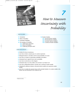
ВЇ = .67. We are asked to find P (AB C),
ВЇ the shaded region in Figure
.13, P (ABC) = .1, and P (AВЇB
4.4 Filling in this information on a Venn diagram, in the order indicated by (1), (2), (3), etc.
31
Figure 4.4: Venn Diagram for Math Averages Example
(1) given
(2) P (AC) в€’ P (ABC)
(3) P (BC) в€’ P (ABC)
(4) P (C) в€’ P (AC) в€’ .03
(5) unknown
(6) P (A) в€’ P (AC) в€’ x
(7) P (B) в€’ P (BC) в€’ x
(8) given
(Usually, we start filling in at the centre and work our way out.)
ВЇ
Adding all probabilities and noting that P (S) = 1, we can solve to get x = .06 = P (AB C).
Problems:
4.1.1 In a typical year, 20% of the days have a high temperature > 22o C. On 40% of these days there
is no rain. In the rest of the year, when the high temperature ≤ 22o C, 70% of the days have no
rain. What percent of days in the year have rain and a high temperature ≤ 22o C?
4.1.2 According to a survey of people on the last Ontario voters list, 55% are female, 55% are politically to the right, and 15% are male and politically to the left. What percent are female and
politically to the right? Assume voter attitudes are classified simply as left or right.
32
C
A
B
Aв€ЄBв€ЄC
Figure 4.5: The union A в€Є B в€Є C
4.2 Rules for Unions of Events
In addition to the two rules which govern probabilities listed in Section 4.1, we have the following
3. (probability of unions)
(a)
P (A в€Є B) = P (A) + P (B) в€’ P (AB)
This can be obtained by using a Venn diagram. Each point in A в€Є B must be counted once. Since
points in AB are counted twice - once in P (A) and once in P (B) - they need to be subtracted
once.
(b)
P (A в€Є B в€Є C) = P (A) + P (B) + P (C) в€’ [P (AB) + P (AC) + P (BC)] + P (ABC)
(see Figure 4.5)
(c)
P (A1 в€Є A2 в€Є A3 в€Є В· В· В· в€Є An ) =
в€’
(where the subscripts are all different)
This generalization is seldom used in Stat 230.
X
X
P (Ai ) в€’
X
P (Ai Aj ) +
P (Ai Aj Ak Al ) + В· В· В·
X
P (Ai Aj Ak )
33
Definition 5 Events A and B are mutually exclusive if AB = П† (the null set)
Since mutually exclusive events A and B have no common points, P (AB) = 0.
In general, events A1 , A2 В· В· В· , An are mutually exclusive if Ai Aj = П† for all i 6= j. This means
that there is no chance of 2 or more of these events occurring together. For example, if a die is rolled
twice, the events
A = {2 occurs on the 1st roll} and
B = {the total is 10}
are mutually exclusive. In the case of mutually exclusive events, rule 3 above simplifies to rule 4 below.
Exercise:
Think of some pairs of events and classify them as being mutually exclusive or not mutually exclusive.
4. (unions of mutually exclusive events)
(a) Let A and B be mutually exclusive events. Then P (A в€Є B) = P (A) + P (B)
(b) In general, let A1 , A2 , В· В· В· An be mutually exclusive.
n
P
Then P (A1 в€Є A2 в€Є В· В· В· в€Є An ) =
P (Ai )
i=1
Proof: Use rule 3 above
ВЇ
5. (probability of complements) P (A) = 1 в€’ P (A)
Proof:
A and AВЇ are mutually exclusive so
ВЇ = P (A) + P (A).
ВЇ
P (A в€Є A)
But
A в€Є AВЇ = S and P (S) = 1
ВЇ =1
Therefore P (A) + P (A)
ВЇ
P (A) = 1 в€’ P (A)
ВЇ is easier to obtain than P (A).
This result is useful whenever P (A)
34
Example: Two ordinary dice are rolled. Find the probability that at least one of them turns up a 6.
Solution 1: Let A = { 6 on the first die }, B = { 6 on the second die } and note (rule 3) that
P (≥ one 6) = P (A ∪ B)
= P (A) + P (B) в€’ P (AB)
1
= 16 + 16 в€’ 36
= 11
36
Solution 2:
P (≥ one 6) = 1 − P (no 6 on either die)
= 1 в€’ 25
36
= 11
36
Example: Roll a die 3 times. Find the probability of getting at least one 6.
Solution 1:
Let A = {≥ one 6}. Then A¯ = {no 6’s }.
Using counting arguments, there are 6 outcomes on each roll, so S has 6 Г— 6 Г— 6 = 216 points. For AВЇ
to occur we can’t have a 6 on any roll. Then A¯ can occur in 5 × 5 × 5 = 125 ways.
ВЇ = 125 .
Therefore P (A)
216
Hence P (A) = 1 в€’
125
91
=
216
216
Solution 2:
Let
Can you spot the flaw in this?
A = {6 occurs on 1st roll}
B = {6 occurs on 2nd roll}
C = {6 occurs on 3rd roll}.
Then
P (≥ one 6) = P (A ∪ B ∪ C)
= P (A) + P (B) + P (C)
= 16 + 16 + 16 = 12
You should have noticed that A, B, and C are not mutually exclusive events, so we should have used
P (A в€Є B в€Є C) = P (A) + P (B) + P (C) в€’ P (AB) в€’ P (AC) в€’ P (BC) + P (ABC)
Each of AB, AC, and BC occurs only once in the 36 point sample space for those two rolls.
Therefore P (A в€Є B в€Є C) =
1
1
1
1
1 1 1
+ + в€’
в€’
в€’
+
= 91/216.
6 6 6 36 36 36 216
35
Note: Rules 3, 4, and (indirectly) 5 link the concepts of addition, unions and complements. The next
segment will consider intersection, multiplication of probabilities, and a concept known as independence. Making these linkages will make problem solving and the construction of probability models
easier.
Problems:
4.2.1 Let A, B, and C be events for which
P (A) = 0.2, P (B) = 0.5, P (C) = 0.3 and P (AB) = 0.1
(a) Find the largest possible value for P (A в€Є B в€Є C)
(b) For this largest value to occur, are the events A and C mutually exclusive, not mutually
exclusive, or is this unable to be determined?
4.2.2 Prove that P (A в€Є B) = 1 в€’ P (A B) for arbitrary events A and B in S.
4.3 Intersections of Events and Independence
Dependent and Independent Events:
Consider these two groups of pairs of events.
Group 1
A = {airplane engine fails in flight}
B = {airplane reaches its destination safely}
or
(when a fair coin is tossed twice)
A = {H is on 1st toss}
B = {H on both tosses}.
A
B
or
A
B
=
=
=
=
Group 2
{a coin toss shows heads}
{a bridge hand has 4 aces}.
(when a fair coin is tossed twice)
{H on 1st toss}
{H on 2nd toss}
What do the pairs A, B in each group have in common? In group 1 the events are related so that the
occurrence of A affects the chances of B occurring. In group 2, whether A occurs or not has no effect
on B’s occurrence.
36
S
A
P(AB)=P(A)P(B)
B
Figure 4.6: Independent Events A, B
We call the pairs in group 1 dependent events, and those in group 2 independent events. We formalize
this concept in the mathematical definition which follows.
Definition 6 Events A and B are independent if and only if P (AB) = P (A)P (B). If they are not
independent, we call the events dependent.
If two events are independent, then the “size” of their intersection as measured by the probability
measure is required to be the product of the individual probabilities. This means, of course, that the
intersection must be non-empty, and so the events are not mutually exclusive. For example in the Venn
diagram depicted in Figure 4.6, P (A) = 0.3, P (B) = 0.4 and P (AB) = 0.12 so in this case the two
events are independent.
For another example, suppose we toss a fair coin twice. Let A = {head on 1st toss} and B = {head
on 2nd toss}. Clearly A and B are independent since the outcome on each toss is unrelated to other
tosses, so P (A) = 12 , P (B) = 12 , P (AB) = 14 = P (A)P (B).
However, if we roll a die once and let A = {the number is even} and B = {number > 3} the events will
be dependent since
1
2
1
P (A) = , P (B) = , P (AB) = P (4 or 6 occurs) = 6= P (A)P (B).
2
2
6
(Rationale: B only happens half the time. If A occurs we know the number is 2, 4, or 6. So B occurs
2
3 of the time when A occurs. The occurrence of A does affect the chances of B occurring so A and B
are not independent.)
When there are more than 2 events, the above definition generalizes to:
37
Definition 7 The events A1 , A2 , В· В· В· , An are independent if and only if
P (Ai1 , Ai2 , В· В· В· , Aik ) = P (Ai1 )P (Ai2 ) В· В· В· P (Aik )
for all sets (i1 , i2 , В· В· В· , ik ) of distinct subscripts chosen from (1, 2, В· В· В· , n)
For example, for n = 3, we need
P (A1 A2 ) = P (A1 )P (A2 ),
P (A1 A3 ) = P (A1 )P (A3 ),
P (A2 A3 ) = P (A2 )P (A3 )
and
P (A1 A2 A3 ) = P (A1 )P (A2 )P (A3 )
Technically, we have defined “mutually independent” events, but we will shorten the name to “independent” to reduce confusion with “mutually exclusive.”
The definition of independence works two ways. If we can find P (A), P (B), and P (AB) then we can
determine whether A and B are independent. Conversely, if we know (or assume) that A and B are
independent, then we can use the definition as a rule of probability to calculate P (AB). Examples of
each follow.
Example:
Toss a die twice. Let A = {first toss is a 3} and B = {the total is 7}. Are A and B
6
independent? (What do you think?) Using the definition to check, we get P (A) = 16 , P (B) = 36
1
(points (1,6), (2,5), (3,4), (4,3), (5,2) and (6,1) give a total of 7) and P (AB) = 36
(only the point (3,4)
makes AB occur).
Therefore, P (AB) = P (A)P (B) and so A and B are independent events.
Now suppose we change B to the event {total is 8}.
Then
5
1
1
and P (AB) =
P (A) = , P (B) =
6
36
36
Therefore P (AB) 6= P (A)P (B)
and consequently A and B are dependent events.
38
This example often puzzles students. Why are they independent if B is a total of 7 but dependent for a
total of 8? The key is that regardless of the first toss, there is always one number on the 2nd toss which
6
= 16 , the outcome of
makes the total 7. Since the probability of getting a total of 7 started off being 36
the 1st toss doesn’t affect the chances. However, for any total other than 7, the outcome of the 1st toss
does affect the chances of getting that total (e.g., a first toss of 1 guarantees the total cannot be 8).
Example: A (pseudo) random number generator on the computer can give a sequence of independent
1
of
random digits chosen from S = {0, 1, . . . , 9}. This means that (i) each digit has probability of 10
being any of 0, 1, . . . , 9, and (ii) the outcomes for the different trials are independent of one another.
We call this type of setting an “experiment with independent trials”. Determine the probability that
(a) in a sequence of 5 trials, all the digits generated are odd
(b) the number 9 occurs for the first time on trial 10.
Solution:
(a) Define the events Ai = {digits from trial i is odd}, i = 1, . . . , 5.
Then
P (all digits are odd) = P (A1 A2 A3 A4 A5 )
5
Q
P (Ai ),
=
i=1
since the Ai ’s are mutually independent. Since P (Ai ) = .5, we get P (all digits are odd) = .55 .
(b) Define events Ai = {9 occurs on trial i}, i = 1, 2, . . . . Then we want
P (AВЇ1 AВЇ2 . . . AВЇ9 A10 ) = P (AВЇ1 )P (AВЇ2 ) . . . P (AВЇ9 )P (A10 )
= (.9)9 (.1),
because the Ai ’s are independent, and P (Ai ) = .1 = 1 − P (A¯i ).
Note: We have used the fact here that if A and B are independent events, then so are AВЇ and B. To see
this note that
ВЇ
P (AB)
=
=
=
=
P (B) в€’ P (AB)
(use a Venn diagram)
P (B) в€’ P (A)P (B) (since A and B are independent)
(1 в€’ P (A))P (B)
ВЇ (B).
P (A)P
39
Note: We have implicitly assumed independence of events in some of our earlier probability calculations. For example, suppose a coin is tossed 3 times, and we consider the sample space
S = {HHH, HHT, HT H, T HH, HT T, T HT, T T H, T T T }
Assuming that the outcomes on the three tosses are independent, and that
P (H) = P (T ) =
1
2
on any single toss, we get that
1
1
P (HHH) = P (H)P (H)P (H) = ( )3 = .
2
8
Similarly, all the other simple events have probability 18 . Note that in earlier calculations we assumed
this was true without thinking directly about independence. However, it is clear that if somehow the 3
tosses were not independent then it might be a bad idea to assume each simple event had probability
1
8 . (For example, instead of heads and tails, suppose H stands for “rain” and T stands for “no rain” on
a given day; now consider 3 consecutive days. Would you want to assign a probability of 18 to each of
the 8 simple events?)
Note: The definition of independent events can thus be used either to check for independence or,
if events are known to be independent, to calculate P (AB). Many problems are not obvious, and
scientific study is needed to determine if two events are independent. For example, are the events A
and B independent if, for a random child living in a country,
A = {live within 5 km. of a nuclear power plant}
B = {a child has leukemia}?
Such problems, which are of considerable importance, can be handled by methods in later statistics
courses.
Problems:
4.3.1 A weighted die is such that P (1) = P (2) = P (3) = 0.1, P (4) = P (5) = 0.2, and P (6) = 0.3.
(a) If the die is thrown twice what is the probability the total is 9?
(b) If a die is thrown twice, and this process repeated 4 times, what is the probability the total will
be 9 on exactly 1 of the 4 repetitions?
40
4.3.2 Suppose among UW students that 15% speaks French and 45% are women. Suppose also that
20% of the women speak French. A committee of 10 students is formed by randomly selecting
from UW students. What is the probability there will be at least 1 woman and at least 1 French
speaking student on the committee?
4.3.3 Prove that A and B are independent events if and only if A and B are independent.
4.4 Conditional Probability
In many situations we may want to determine the probability of some event A, while knowing that
some other event B has already occurred. For example, what is the probability a randomly selected
person is over 6 feet tall, given that they are female? Let the symbol P (A|B) represent the probability
that event A occurs, when we know that B occurs. We call this the conditional probability of A given
B. While we will give a definition of P (A|B), let’s first consider an example we looked at earlier, to
get some sense of why P (A|B) is defined as it is.
Example: Suppose we roll a die once. Let A = {the number is even} and B = {number > 3}. If we
know that B occurs, that tells us that we have a 4, 5, or 6. Of the times when B occurs, we have an
even number 23 of the time. So P (A|B) = 23 . More formally, we could obtain this result by calculating
P (AB)
2
3
P (B) , since P (AB) = P (4 or 6) = 6 and P (B) = 6 .
Definition 8 the conditional probability of event A, given event B, is
P (A|B) =
P (AB)
, provided P (B) 6= 0.
P (B)
Note: If A and B are independent,
P (AB) = P (A)P (B) so
P (A|B) =
P (A)P (B)
= P (A).
P (B)
This makes sense, and can be taken as an equivalent definition of independence; that is, A and B are
independent iff P (A|B) = P (A). You should investigate the behaviour of the conditional probabilities
as we move the events around on the web-site http://stat-www.berkeley.edu/%7Estark/Java/Venn3.htm.
Example: If a fair coin is tossed 3 times, find the probability that if at least 1 Head occurs, then
exactly 1 Head occurs.
Solution:
Define the events A = {1 Head}, B = {at least 1 Head}. What we are being asked to find
41
is P (A|B). This equals P (AB)/P (B), and so we find
P (B) = 1 в€’ P (0 Heads) =
7
8
and
P (AB) = P {1 Head} = P ({HT T, T HT, T T H})
= 38
using either the sample space with 8 points, or the fact that the 3 tosses are independent. Thus,
P (A|B) =
3
8
7
8
3
= .
7
Example: The probability a randomly selected male is colour-blind is .05, whereas the probability a
female is colour-blind is only .0025. If the population is 50% male, what is the fraction that is colourblind?
Solution:
Let
C = {person selected is colour-blind}
M = {person selected is male}
F = {person selected is female}
We are asked to find P (C). We are told that
P (C|M ) = 0.05,
P (C|F ) = 0.0025,
P (M ) = 0.5 = P (F ).
To get P (C) we can therefore use
P (C) = P (CM ) + P (CF )
= P (C|M )P (M ) + P (C|F )P (F )
= (0.05)(0.5) + (0.0025)(0.05)
= 0.02625.
4.5 Multiplication and Partition Rules
The preceding example suggests two more probability rules, which turn out to be extremely useful.
They are based on breaking events of interest into pieces.
6. Multiplication Rules
Let A, B, C, D, . . . be arbitrary events in a sample space. Then
P (AB) = P (A)P (B|A)
P (ABC) = P (A)P (B|A)P (C|AB)
P (ABCD) = P (A)P (B|A)P (C|AB)P (D|ABC)
42
and so on.
Proof:
The first rule comes directly from the definition P (B|A). The right hand side of the second rule
equals (assuming P (AB) 6= 0)
P (AB)P (C|AB) = P (AB)
P (CAB)
= P (ABC),
P (AB)
and so on.
Partition Rule
Let A1 , . . . , Ak be a partition of the sample space S into disjoint (mutually exclusive) events such that
A1 в€Є A2 в€Є В· В· В· в€Є Ak = S.
Let B be an arbitrary event in S. Then
P (B) = P (BA1 ) + P (BA2 ) + В· В· В· + P (BAk )
k
P
=
P (B|Ai )P (Ai )
i=1
Proof: Look at a Venn diagram to see that BA1 , . . . , BAk are mutually exclusive, with B = (BA1 ) в€Є
В· В· В· в€Є (BAk ).
Example: In an insurance portfolio 10% of the policy holders are in Class A1 (high risk), 40% are
in Class A2 (medium risk), and 50% are in Class A3 (low risk). The probability a Class A1 policy has
a claim in a given year is .10; similar probabilities for Classes A2 and A3 are .05 and .02. Find the
probability that if a claim is made, it is for a Class A1 policy.
Solution: For a randomly selected policy, let
B = {policy has a claim }
Ai = {policy is of Class Ai }, i = 1, 2, 3
We are asked to find P (A1 |B). Note that
P (A1 |B) =
P (A1 B)
P (B)
and that
P (B) = P (A1 B) + P (A2 B) + P (A3 B).
We are told that
P (A1 ) = 0.10, P (A2 ) = 0.40, P (A3 ) = 0.50
43
and that
P (B|A1 ) = 0.10, P (B|A2 ) = 0.05, P (B|A3 ) = 0.02.
Thus
P (A1 B) = P (A1 )P (B|A1 ) = .01
P (A2 B) = P (A2 )P (B|A2 ) = .02
P (A3 B) = P (A3 )P (B|A3 ) = .01
Therefore P (B) = .04 and P (A1 |B) = .01/.04 = .25.
Tree Diagrams
Tree diagrams can be a useful device for keeping track of conditional probabilities when using multiplication and partition rules. The idea is to draw a tree where each path represents a sequence of
events. On any given branch of the tree we write the conditional probability of that event given all the
events on branches leading to it. The probability at any node of the tree is obtained by multiplying the
probabilities on the branches leading to the node, and equals the probability of the intersection of the
events leading to it.
For example, the immediately preceding example could be represented by the tree in Figure 4.7.
Note that the probabilities on the terminal nodes must add up to 1.
Here is another example involving diagnostic tests for disease. See if you can represent the problem by
a tree.
Example. Testing for HIV
Tests used to diagnose medical conditions are often imperfect, and give false positive or false negative
results, as described in Problem 2.6 of Chapter 2. A fairly cheap blood test for the Human Immunodeficiency Virus (HIV) that causes AIDS (Acquired Immune Deficiency Syndrome) has the following
characteristics: the false negative rate is 2% and the false positive rate is 0.5%. It is assumed that
around .04% of Canadian males are infected with HIV.
Find the probability that if a male tests positive for HIV, he actually has HIV.
Solution: Suppose a male is randomly selected from the population, and define the events
A = {person has HIV}
B = {blood test is positive}
We are asked to find P (A|B). From the information given we know that
ВЇ = .9996
P (A) = .0004, P (A)
ВЇ = .005
P (B|A) = .98, P (B|A)
44
P(A1B) =.01
P(B|A1) =.1
.9
P(A1B) =.09
P(A ) =.1
1
P(B|A ) =.05
P(A B) =.02
2
2
P(A ) =.4
2
.95
P(A2B) =.38
P(A ) =.5
3
P(B|A ) =.02
P(A3B) =.01
3
.98
P(A3B) =.49
Figure 4.7:
Therefore we can find
P (AB) = P (A)P (B|A)
= .000392
ВЇ
ВЇ
ВЇ
P (AB) = P (A)P (B|A)
= .004998
ВЇ
Therefore
P (B) = P (AB) + P (AB) = .00539
and
P (A|B) =
P (AB)
= .0727
P (B)
Thus, if a randomly selected male tests positive, there is still only a small probability (.0727) that they
actually have HIV!
Exercise: Try to explain in ordinary words why this is the case.
Note: Bayes Theorem
By using the definition of conditional probability and the multiplication rule, we get that
P (A|B) =
P (AB)
P (B|A)P (A)
=
P (B)
P (B)
This result is called Bayes Theorem, after a mathematician3 who proved it in the 1700’s. It is a very
trivial theorem, but it has inspired approaches to problems in statistics and other areas such as machine
3
(Rev) Thomas Bayes (1702-1761) was an English Nonconformist minister, turned Presbyterian. He may have been
45
learning, classification and pattern recognition. In these areas the term “Bayesian methods” is often
used.
Problems:
4.4.1 If you take a bus to work in the morning there is a 20% chance you’ll arrive late. When you go
by bicycle there is a 10% chance you’ll be late. 70% of the time you go by bike, and 30% by
bus. Given that you arrive late, what is the probability you took the bus?
4.4.2 A box contains 4 coins – 3 fair coins and 1 biased coin for which P (heads) = .8. A coin is picked
at random and tossed 6 times. It shows 5 heads. Find the probability this coin is fair.
4.4.3 At a police spot check, 10% of cars stopped have defective headlights and a faulty muffler. 15%
have defective headlights and a muffler which is satisfactory. If a car which is stopped has
defective headlights, what is the probability that the muffler is also faulty?
4.6 Problems on Chapter 4
4.1 If A and B are mutually exclusive events with P (A) = 0.25 and P (B) = 0.4, find the probability
of each of the following events:
ВЇ B;
¯ A ∪ B; A ∩ B; A¯ ∪ B;
¯ A¯ ∩ B;
¯ A ∩ B.
A;
4.2 Three digits are chosen at random with replacement from 0, 1, ..., 9; find the probability of each
of the following events.
A: “all three digits are the same”;
B: “all three digits are different”;
C: “the digits are all nonzero”;
D: “the digits all exceed 4”;
E “digits all have the same parity (all odd or all even)”.
Then find the probability of each of the following events, which are combinations of the previous
five events:
BE; B в€Є D; B в€Є D в€Є E; (A в€Є B)D; A в€Є (BD).
Show the last two of these events in Venn diagrams.
4.3 Let A and B be events defined on the same sample space, with P (A) = 0.3, P (B) = 0.4 and
P (A|B) = 0.5. Given that event B does not occur, what is the probability of event A?
tutored by De Moivre. His famous paper introducing this rule was published after his death. “Bayesians” are statisticians
who opt for a purely probabilistic view of inference. All unknowns obtain from some distribution and ultimately, the
distribution says it all.
46
4.4 A die is loaded to give the probabilities:
number
1
2
3
4
5
6
probability
.3
.1
.15
.15
.15
.15
The die is thrown 8 times. Find the probability
(a) 1 does not occur
(b) 2 does not occur
(c) neither 1 nor 2 occurs
(d) both 1 and 2 occur.
4.5 Events A and B are independent with P (A) = .3 and P (B) = .2. Find P (A в€Є B).
4.6 Students A, B and C each independently answer a question on a test. The probability of getting
the correct answer is .9 for A, .7 for B and .4 for C. If 2 of them get the correct answer, what is
the probability C was the one with the wrong answer?
4.7 70% of the customers buying at a certain store pay by credit card. Find the probability
(a) 3 out of 5 customers pay by credit card
(b) the 5th customer is the 3rd one to pay by credit card.
4.8 Let E and F be independent with E = A в€Є B and F = AB. Prove that either P (AB) = 0 or
Вў
ВЎ
else P A B = 0.
4.9 In a large population, people are one of 3 genetic types A, B and C: 30% are type A, 60% type
B and 10% type C. The probability a person carries another gene making them susceptible for
a disease is .05 for A, .04 for B and .02 for C. If ten unrelated persons are selected, what is the
probability at least one is susceptible for the disease?
4.10 Two baseball teams play a best-of-seven series, in which the series ends as soon as one team wins
four games. The first two games are to be played on A’s field, the next three games on B’s field,
and the last two on A’s field. The probability that A wins a game is 0.7 at home and 0.5 away.
Find the probability that:
(a) A wins the series in 4 games; in 5 games;
(b) the series does not go to 6 games.
47
4.11 A population consists of F females and M males; the population includes f female smokers and
m male smokers. An individual is chosen at random from the population. If A is the event that
this individual is female and B is the event he or she is a smoker, find necessary and sufficient
conditions on f , m, F and M so that A and B are independent events.
4.12 An experiment has three possible outcomes A, B and C with respective probabilities p, q and r,
where p + q + r = 1. The experiment is repeated until either outcome A or outcome B occurs.
Show that A occurs before B with probability p/(p + q).
4.13 In the game of craps, a player rolls two dice. They win at once if the total is 7 or 11, and lose at
once if the total is 2, 3, or 12. Otherwise, they continue rolling the dice until they either win by
throwing their initial total again, or lose by rolling 7.
Show that the probability they win is 0.493.
(Hint: You can use the result of Problem 4.12)
4.14 A researcher wishes to estimate the proportion p of university students who have cheated on an
examination. The researcher prepares a box containing 100 cards, 20 of which contain Question
A and 80 Question B.
Question A: Were you born in July or August?
Question B: Have you ever cheated on an examination?
Each student who is interviewed draws a card at random with replacement from the box and
answers the question it contains. Since only the student knows which question he or she is answering, confidentiality is assured and so the researcher hopes that the answers will be truthful4 .
It is known that one-sixth of birthdays fall in July or August.
(a) What is the probability that a student answers �yes’?
(b) If x of n students answer �yes’, estimate p.
(c) What proportion of the students who answer �yes’ are responding to Question B?
4.15 Diagnostic tests. Recall the discussion of diagnostic tests in Problem 2.6 for Chapter 2. For a
randomly selected person let D = �person has the disease’ and R = �the test result is positive’.
ВЇ P (R).
Give estimates of the following probabilities: P (R|D), P (R|D),
4.16 Slot machines. Standard slot machines have three wheels, each marked with some number of
symbols at equally spaced positions around the wheel. For this problem suppose there are 10
positions on each wheel, with three different types of symbols being used: flower, dog, and
house. The three wheels spin independently and each has probability 0.1 of landing at any
4
"A foolish faith in authority is the worst enemy of truth" Albert Einsten, 1901.
48
position. Each of the symbols (flower, dog, house) is used in a total of 10 positions across the
three wheels. A payout occurs whenever all three symbols showing are the same.
(a) If wheels 1, 2, 3 have 2, 6, and 2 flowers, respectively, what is the probability all three
positions show a flower?
(b) In order to minimize the probability of all three positions showing a flower, what number
of flowers should go on wheels 1, 2 and 3? Assume that each wheel must have at least one
flower.
4.17 Spam detection 1. Many methods of spam detection are based on words or features that appear
much more frequently in spam than in regular email. Conditional probability methods are then
used to decide whether an email is spam or not. For example, suppose we define the following
events associated with a random email message.
Spam = “Message is spam”
Not Spam = “Message is not spam (“regular”)”
A = “Message contains the word Viagra”
If we know the values of the probabilities P (Spam), P (A| Spam) and P (A| Not Spam), then
we can find the probabilities P (Spam|A) and P (Not Spam|A).
(a) From a study of email messages coming into a certain system it is estimated that P (Spam)
= .5, P (A|Spam) = .2, and P (A|Not Spam) = .001. Find P (Spam|A) and P (Not Spam|A).
(b) If you declared that any email containing the word Viagra was Spam, then find what fraction
of regular emails would be incorrectly identified as Spam.
4.18 Spam detection 2. The method in part (b) of the preceding question would only filter out 20% of
Spam messages. (Why?) To increase the probability of detecting spam, we can use a larger set of
email “features”; these could be words or other features of a message which tend to occur with
much different probabilities in spam and in regular email. (From your experience, what might be
some useful features?) Suppose we identify n binary features, and define events
Ai = feature i appears in a message.
We will assume that A1 , . . . , An are independent events, given that a message is spam, and that
they are also independent events, given that a message is regular.
Suppose n = 3 and that
P (A1 |Spam) = .2
P (A1 |Not Spam) = .005
P (A2 |Not Spam) = .004
P (A2 |Spam) = .1
P (A3 |Not Spam) = .005
P (A3 |Spam) = .1
Assume as in the preceding question that P (Spam) = .5.
49
(a) Suppose a message has all of features 1, 2, and 3 present. Determine P (Spam |A1 A2 A3 ).
(b) Suppose a message has features 1 and 2 present, but feature 3 is not present. Determine
P (Spam |A1 A2 AВЇ3 ).
(c) If you declared as spam any message with one or more of features 1, 2 or 3 present, what
fraction of spam emails would you detect?
4.19 Online fraud detection. Methods like those in problems 4.17 and 4.18 are also used in monitoring events such as credit card transactions for potential fraud. Unlike the case of spam email,
however, the fraction of transactions that are fraudulent is usually very small. What we hope to
do in this case is to “flag” certain transactions so that they can be checked for potential fraud, and
perhaps to block (deny) certain transactions. This is done by identifying features of a transaction
so that if F = “transaction is fraudulent”, then
r=
P (feature present|F )
P (feature present|FВЇ )
is large.
(a) Suppose P (F ) =0.0005 and that P (feature present|FВЇ ) = .02. Determine P (F | feature
present) as a function of r, and give the values when r = 10,30 and 100.
(b) Suppose r = 100 and you decide to flag transactions with the feature present. What percentage of transactions would be flagged? Does this seem like a good idea?
50
5. Review of Useful Series and Sums
The preceding chapters have introduced ways to calculate the probabilities of random events, based on
various assumptions. You may have noticed that many of the problems you’ve encountered are actually
similar, despite the contexts being different. Our approach in the next few chapters will be to classify
some of these common types of problems and develop general methods for handling them. Rather
than working each problem out as if we’d never seen one like it before, our emphasis will now shift to
checking whether the problem is one of these general types.
5.1 Series and Sums
Before starting on the probability models of the next chapter, it’s worth reviewing some useful results
for series, and for summing certain series algebraically. We’ll be making use of them in the next few
chapters, and many, such as the geometric series, have already been used.
1. Geometric Series:
a + ar + ar2 + В· В· В· + arnв€’1 =
If |r| < 1, then
a (rn в€’ 1)
a (1 в€’ rn )
=
for r 6= 1
1в€’r
rв€’1
a + ar + ar2 + В· В· В· =
a
1в€’r
2. Binomial Theorem: There are various forms of this theorem. We’ll use the form
n Вµ В¶
X
n x
a .
(1 + a)n =
x
x=0
In a more general version, when n is not a positive integer,
в€ћ Вµ В¶
X
n x
n
a if |a| < 1.
(1 + a) =
x
x=0
ВЎ Вў
(We have already defined nx when n is not a positive integer.) While the binomial theorem may
в€ћ ВЎ Вў
P
n x
not look like a summation result, we’ll use it to evaluate series of the form
x a .
x=0
51
52
3. Multinomial Theorem: A generalization of the binomial theorem is
X
n!
ax1 ax2 В· В· В· axkk .
x1 !x2 ! В· В· В· xk ! 1 2
P
with the summation over all x1 , x2 , В· В· В· , xk with xi = n. The case k = 2 gives the binomial
theorem in the form
n Вµ В¶
X
n x1 nв€’x1
(a1 + a2 )n =
a1 a2
x
1
x =0
(a1 + a2 + В· В· В· + ak )n =
1
.
4. Hypergeometric Identity:
В¶ Вµ
В¶
∞ µ ¶µ
X
a
b
a+b
=
.
x nв€’x
n
x=0
There will not be an infinite number of terms if a and b are positive integers since the terms
become 0 eventually. For example
Вµ В¶
4
4 (5) (4)(3)(2)(1)(0)
=0
=
=
5!
5!
5
Sketch of Proof:
(1 + y)a+b = (1 + y)a (1 + y)b .
Expand each term by the binomial theorem and equate the coefficients of y n on each side.
5. Exponential series:
ex =
в€ћ
X
xn
x0 x1 x2 x3
+
+
+
+ В·В·В· =
0!
1!
2!
3!
n!
n=0
(Recall, also that
Ві
x Вґn
1+
)
n→∞
n
ex = lim
6. Special series involving integers:
n(n + 1)
2
n(n + 1)(2n + 1)
2
2
2
2
1 + 2 + 3 + В·В·В· + n =
6
Вё
в€™
n(n + 1) 2
3
3
3
3
1 + 2 + 3 + В·В·В· + n =
2
1 + 2 + 3 + В·В·В· +n =
53
Example: Find
µ ¶µ
В¶
a
b
x (x в€’ 1)
x nв€’x
x=0
в€ћ
X
Solution: For x = 0 or 1 the term becomes 0, so we can start summing at x = 2. For x ≥ 2, we
can expand x! as x(x в€’ 1)(x в€’ 2)!
В¶ X
В¶
Вµ
µ ¶µ
в€ћ
в€ћ
X
b
b
a
a!
=
.
x(x в€’ 1)
x(x в€’ 1)
x nв€’x
x(x в€’ 1)(x в€’ 2)!(a в€’ x)! n в€’ x
x=0
x=2
Cancel the x(x − 1) terms and try to re-group the factorial terms as “something choose something”.
Вµ
В¶
a!
a(a в€’ 1)(a в€’ 2)!
aв€’2
=
= a(a в€’ 1)
.
(x в€’ 2)!(a в€’ x)!
(x в€’ 2)! [(a в€’ 2) в€’ (x в€’ 2)]!
xв€’2
Then
µ ¶µ
В¶ X
Вµ
¶µ
В¶
в€ћ
a
b
aв€’2
b
x(x в€’ 1)
=
a(a в€’ 1)
.
x nв€’x
xв€’2 nв€’x
x=0
x=2
в€ћ
X
Factor out a(a в€’ 1) and let y = x в€’ 2 to get
В¶
В¶
Вµ
¶µ
в€ћ Вµ
X
a+bв€’2
b
aв€’2
= a(a в€’ 1)
a(a в€’ 1)
nв€’2
n в€’ (y + 2)
y
y=0
by the hypergeometric identity.
5.2 Problems on Chapter 5
(Solutions to 5.1 and 5.2 are given in Chapter 10.)
5.1 Show that
(use the binomial theorem).
Вµ В¶
n
X
n x
x
p (1 в€’ p)nв€’x = np
x
x=0
5.2 I have a quarter which turns up heads with probability 0.6, and a fair dime. Both coins are tossed
simultaneously and independently until at least one shows heads. Find the probability that both
the dime and the quarter show heads at the same time.
5.3 Some other summation formulas can be obtained by differentiating the above equations on both
a
sides. Show that a + 2ar + 3ar2 + В· В· В· = (1в€’r)
2 by starting with the geometric series formula.
Assume |r| < 1.
54
5.4 Players A and B decide to play chess until one of them wins. Assume games are independent
with P (A wins) = .3, P (B wins) = .25 and P (draw) = .45 on each game. If the game ends in a
draw another game will be played. Find the probability A wins before B.
6. Discrete Random Variables and
Probability Models
6.1 Random Variables and Probability Functions
Probability models are used to describe outcomes associated with random processes. So far we have
used sets A, B, C, . . . in sample spaces to describe such outcomes. In this chapter we introduce
numerical-valued variables X, Y, . . . to describe outcomes. This allows probability models to be manipulated easily using ideas from algebra, calculus, or geometry.
A random variable (r.v.) is a numerical-valued variable that represents outcomes in an experiment or
random process. For example, suppose a coin is tossed 3 times; then
X = Number of Heads that occur
would be a random variable. Associated with any random variable is a range or domain A, which is
the set of possible values for the variable. For example, the random variable X defined above has range
A = {0, 1, 2, 3}.
Random variables are denoted by capital letters like X, Y, . . . and their possible values are denoted by
x, y, . . . . This gives a nice short-hand notation for outcomes: for example, “X = 2” in the experiment
above stands for “2 heads occurred”.
Random variables are always defined so that if the associated random process or experiment is carried
out, then one and only one of the outcomes “X = x”(x ∈ A) occurs. In other words, the possible
values for X form a partition of the points in the sample space for the experiment. In more advanced
mathematical treatments of probability, a random variable is defined as a function on a sample space,
as follows:
Definition 9 A random variable is a function that assigns a real number to each point in a sample
space S.
To understand this definition, consider the experiment in which a coin is tossed 3 times, and suppose
55
56
that we used the sample space
S = {HHH, T HH, HT H, HHT, HT T, T HT, T T H, T T T }.
Then each of the outcomes “X = x” (where X = number of heads) represents an event (either simple or compound) and so a real number x can be associated with each point in S. In particular, the
point HHH corresponds to x = 3; the points T HH, HT H, HHT correspond to x = 2; the points
HT T, T HT, T T H correspond to x = 1; and the point T T T corresponds to x = 0.
As you may recall, a function is a mapping of each point in a domain into a unique point. e.g. The
function y = x3 maps the point x = 2 in the domain into the point y = 8 in the range. We are familiar
with this rule for mapping being defined by a mathematical formula. However, the rule for mapping a
point in the sample space (domain) into the real number in the range of a random variable is most often
given in words rather than by a formula. As mentioned above, we generally denote random variables,
in the abstract, by capital letters (X, Y , etc.) and denote the actual numbers taken by random variables
by small letters (x, y, etc.). You may, in your earlier studies, have had this distinction made between a
function (X) and the value of a function (x).
Since “X = x” represents an outcome of some kind, we will be interested in its probability, which we
write as P (X = x). To discuss probabilities for random variables, it is easiest if they are classified into
two types, according to their ranges:
Discrete random variables take integer values or, more generally, values in a countable set (recall that
a set is countable if its elements can be placed in a one-one correspondence with a subset of the positive
integers).
Continuous random variables take values in some interval of real numbers.
Examples might be:
Discrete
number of people in a car
number of cars in a parking lot
number of phone calls to 911
Continuous
total weight of people in a car
distance between cars in a parking lot
time between calls to 911.
In theory there could also be mixed r.v.’s which are discrete-valued over part of their range and continuousvalued over some other portion of their range. We will ignore this possibility here and concentrate first
on discrete r.v.’s. Continuous r.v.’s are considered in Chapter 9.
Our aim is to set up general models which describe how the probability is distributed among the possible values a random variable can take. To do this we define for any discrete random variable X the
probability function.
57
Definition 10 The probability function (p.f.) of a random variable X is the function
f (x) = P (X = x), defined for all x в€€ A.
The set of pairs {(x, f (x)) : x в€€ A} is called the probability distribution of X. All probability
functions must have two properties:
1. f (x) ≥ 0 for all values of x (i.e. for x ∈ A)
P
f (x) = 1
2.
all xв€€A
By implication, these properties ensure that f (x) ≤ 1 for all x. We consider a few “toy” examples
before dealing with more complicated problems.
Example 1: Let X be the number obtained when a die is thrown. We would normally use the
probability function f (x) = 1/6 for x = 1, 2, 3, В· В· В· , 6. In fact there probably is no absolutely perfect
die in existence. For most dice, however, the 6 sides will be close enough to being equally likely that
f (x) = 1/6 is a satisfactory model for the distribution of probability among the possible outcomes.
Example 2: Suppose a “fair” coin is tossed 3 times, and let X be the number of heads occurring.
Then a simple calculation using the ideas from earlier chapters gives
ВЎ3Вў
x
f (x) = P (X = x) =
Note that instead of writing f (0) =
algebraic expression.
1
8 , f (1)
=
8
for x = 0, 1, 2, 3.
3
8 , f (2)
=
3
8 , f (3)
=
1
8,
we have given a simple
Example 3: Find the value of k which makes f (x) below a probability function.
Using
3
P
x
0
1
2
3
f (x)
k
2k
0.3
4k
f (x) = 1 gives 7k + 0.3 = 1. Hence k = 0.1.
x=0
While the probability function is the most common way of describing a probability model, there are
other possibilities. One of them is by using the cumulative distribution function (c.d.f.).
Definition 11 The cumulative distribution function of X is the function usually denoted by F (x)
F (x) = P (X ≤ x)
defined for all real numbers x.
58
2
1.8
1.6
1.4
F(x)
1.2
1
f(3)
0.8
0.6
0.4
0.2
0
в€’1
в€’0.5
0
0.5
1
1.5
2
2.5
3
3.5
4
x
Figure 6.1: A simple cumulative distribution function
In the last example, with k = 0.1, we have for x в€€ A
x
0
1
2
3
F (x)
0.1
0.3
0.6
1
since, for instance,
F (2) = P (X ≤ 2) = f (0) + f (1) + f (2) = 0.6.
Similarly, F (x) can be defined for real numbers x not in the range of the random variable, for example
F (2.5) = F (2) = 0.6 and F (3.8) = 1.
The c.d.f. for this example is plotted in Figure 6.1.
In general, F (x) can be obtained from f (x) by the fact that
F (x) = P (X ≤ x) =
X
f (u).
u≤x
A c.d.f. F (x) has certain properties, just as a probability function f (x) does. Obviously, since it
represents a probability, F (x) must be between 0 and 1. In addition it must be a non-decreasing
function (e.g. P (X ≤ 8) cannot be less than P (X ≤ 7)). Thus we note the following properties of a
c.d.f. F (x):
1. F (x) is a non-decreasing function of x.
2. 0 ≤ F (x) ≤ 1 for all x.
59
3. limx→−∞ F (x) = 0 and limx→∞ F (x) = 1.
We have noted above that F (x) can be obtained from f (x). The opposite is also true; for example
the following result holds:
If X takes on integer values then for values x such that x в€€ A and x в€’ 1 в€€ A,
f (x) = F (x) в€’ F (x в€’ 1)
This says that f (x) is the size of the jump in F (x) at the point x.
To prove this, just note that
F (x) − F (x − 1) = P (X ≤ x) − P (X ≤ x − 1) = P (X = x).
When a random variable has been defined it is sometimes simpler to find its probability function (p.f.)
f (x) first, and sometimes it is simpler to find F (x) first. The following example gives two approaches
for the same problem.
Example: Suppose that N balls labelled 1, 2, . . . , N are placed in a box, and n balls (n ≤ N ) are
randomly selected without replacement. Define the r.v.
X = largest number selected
Find the probability function for X.
Solution 1: If X = x then we must select the number x plus nв€’1 numbers from the set {1, 2, . . . , xв€’
1}. (Note that this means we need x ≥ n.) This gives
ВЎxв€’1Вў
ВЎ1ВўВЎxв€’1Вў
f (x) = P (X = x) =
1
ВЎNnв€’1
Вў = ВЎnв€’1
NВў
n
x = n, n + 1, . . . , N
n
Solution 2: First find F (x) = P (X ≤ x). Noting that X ≤ x if and only if all n balls selected are
from the set {1, 2, . . . , x}, we get
ВЎx Вў
n
F (x) = ВЎN
Вў x = n, n + 1, . . . N
n
We can now find
f (x) = F (x) в€’ F (x в€’ 1)
ВЎxВў ВЎxв€’1Вў
в€’
= n ВЎN Вў n
ВЎxв€’1Вўn
= ВЎnв€’1
NВў
n
60
0.4
0.35
0.3
f(x)
0.25
0.2
0.15
0.1
0.05
0
0
1
2
3
x
Figure 6.2: Probability histogram for f (x) =
x+1
10 , x
= 0, 1, 2, 3
as before.
Remark: When you write down a probability function or a cumulative distribution function, don’t
forget to give the range of the function (i.e. the possible values of the random variable). This is part of
the function’s definition.
Sometimes we want to graph a probability function f (x). The type of graph we will use most is
called a (probability) histogram. For now, we’ll define this only for r.v.’s whose range is some set of
consecutive integers {0, 1, 2, . . . }. A histogram of f (x) is then a graph consisting of adjacent bars or
rectangles. At each x we place a rectangle with base on (x в€’ .5, x + .5) and with height f (x). In the
above Example 3, a histogram of f (x) looks like that in Figure 6.2.
Notice that the areas of these rectangles correspond to the probabilities, so for example P (1 ≤ X ≤
3) is the sum of the area of the three rectangles above the points 1, 2, and 3. In general, probabilities
are depicted by areas.
Model Distributions:
Many processes or problems have the same structure. In the remainder of this course we will
identify common types of problems and develop probability distributions that represent them. In doing
this it is important to be able to strip away the particular wording of a problem and look for its essential
features. For example, the following three problems are all essentially the same.
(a) A fair coin is tossed 10 times and the “number of heads obtained” (X) is recorded.
(b) Twenty seeds are planted in separate pots and the “number of seeds germinating” (X) is recorded.
61
(c) Twelve items are picked at random from a factory’s production line and examined for defects.
The number of items having no defects (X) is recorded.
What are the common features? In each case the process consists of “trials" which are repeated a stated
number of times - 10, 20, and 12. In each repetition there are two types of outcomes - heads/tails,
germinate/don’t germinate, and no defects/defects. These repetitions are independent (as far as we can
determine), with the probability of each type of outcome remaining constant for each repetition. The
random variable we record is the number of times one of these two types of outcome occurred.
Six model distributions for discrete r.v.’s will be developed in the rest of this chapter. Students often
have trouble deciding which one (if any) to use in a given setting, so be sure you understand the physical
setup which leads to each one. Also, as illustrated above you will need to learn to focus on the essential
features of the situation as well as the particular content of the problem.
Statistical Computing
A number of major software systems have been developed for probability and statistics. We will use
a system called R, which has a wide variety of features and which has Unix and Windows versions.
Appendix 6.1 at the end of this chapter gives a brief introduction to R, and how to access it. For this
course, R can compute probabilities for all the distributions we consider, can graph functions or data,
and can simulate random processes. In the sections below we will indicate how R can be used for some
of these tasks.
Problems:
6.1.1 Let X have probability function
x
0
1
2
f (x) 9c2 9c c2
. Find c.
6.1.2 Suppose that 5 people, including you and a friend, line up at random. Let X be the number of
people standing between you and your friend. Tabulate the probability function and the cumulative distribution function for X.
6.2 Discrete Uniform Distribution
We define each model in terms of an abstract “physical setup", or setting, and then consider specific
examples of the setup.
Physical Setup: Suppose X takes values a, a + 1, a + 2, В· В· В· , b with all values being equally likely.
Then X has a discrete uniform distribution, on [a, b].
Illustrations:
62
1. If X is the number obtained when a die is rolled, then X has a discrete uniform distribution with
a = 1 and b = 6.
2. Computer random number generators give uniform [1, N ] variables, for a specified positive integer N . These are used for many purposes, e.g. generating lottery numbers or providing automated random sampling from a set of N items.
Probability Function: There are b в€’a + 1 values X can take so the probability at each of these values
b
P
1
in order that
f (x) = 1. Therefore
must be bв€’a+1
x=a
f (x) =
(
1
bв€’a+1 ;
0;
x = a, a + 1, В· В· В· , b
otherwise
Problem 6.2.1
Let X be the largest number when a die is rolled 3 times. First find the c.d.f., F (x), and then find the
probability function, f (x).
6.3 Hypergeometric Distribution
Physical Setup: We have a collection of N objects which can be classified into two distinct types.
Call one type “success”5 (S) and the other type “failure” (F ). There are r successes and N −r failures.
Pick n objects at random without replacement. Let X be the number of successes obtained. Then X
has a hypergeometric distribution.
Illustrations:
1. The number of aces X in a bridge hand has a hypergeometric distribution with N = 52, r = 4,
and n = 13.
2. In a fleet of 200 trucks there are 12 which have defective brakes. In a safety check 10 trucks
are picked at random for inspection. The number of trucks X with defective brakes chosen for
inspection has a hypergeometric distribution with N = 200, r = 12, n = 10.
5
"If A is a success in life, then A equals x plus y plus z. Work is x; y is play; and z is keeping your mouth shut." Albert
Einstein, 1950
63
ВЎ Вў
Probability Function: Using counting techniques we note there are N
n points in the sample space
ВЎr Вў
S if we don’t consider order of selection. There are x ways to choose the x success objects from the
Вў
ВЎ
r available and Nв€’r
nв€’x ways to choose the remaining (n в€’ x) objects from the (N в€’ r) failures. Hence
f (x) =
ВЎr ВўВЎN в€’rВў
x
ВЎNnв€’x
Вў
n
The range of values for x is somewhat complicated. Of course, x ≥ 0. However if the number, n,
picked exceeds the number, N в€’ r, of failures, the difference, n в€’ (N в€’ r) must be successes. So
x ≥ max(0, n − N + r). Also, x ≤ r since we can’t get more successes than the number available. But
x ≤ n, since we can’t get more successes than the number of objects chosen. Therefore x ≤ min(r, n).
Example: In Lotto 6/49 a player selects a set of six numbers (with no repeats) from the set {1, 2, . . . , 49}.
In the lottery draw six numbers are selected at random. Find the probability function for X, the number
from your set which are drawn.
Solution: Think of your numbers as the S objects and the remainder as the F objects. Then X has a
hypergeometric distribution with N = 49, r = 6 and n = 6, so
ВЎ6ВўВЎ 43 Вў
P (X = x) = f (x) =
x
ВЎ496в€’x
Вў , for x = 0, 1, . . . , 6
6
For example, you win the jackpot prize if X = 6; the probability of this is
million.
ВЎ6Вў ВЎ49Вў
6 / 6 , or about 1 in 13.9
Remark: Hypergeometric probabilities are tedious to compute using a calculator. The R functions
dhyper and phyper can be used to evaluate f (x) and the c.d.f F (x). In particular, dhyper(x, r, N в€’
r, n) gives f (x) and phyper(x, r, N в€’ r, n) gives F (x). Using this we find for the Lotto 6/49 problem
here, for example, that f (6) is calculated by typing dhyper(6, 6, 43, 6) in R, which returns the answer
7.151124 Г— 10в€’8 or 1/13, 983, 186.
For all of our model distributions we can also confirm that
P
f (x) = 1. To do this here we use a
all x
summation result from Chapter 5 called the hypergeometric identity. Letting a = r, b = N в€’ r in that
identity we get
ВЎ ВўВЎ
Вў
µ ¶µ
В¶ ВЎr+Nв€’rВў
X xr Nв€’r
X
1 X r
N в€’r
nв€’x
n
= ВЎN Вў
= ВЎN
f (x) =
ВЎN Вў
Вў =1
x
n
в€’
x
n
n
n
all x
64
Problems:
6.3.1 A box of 12 tins of tuna contains d which are tainted. Suppose 7 tins are opened for inspection
and none of these 7 is tainted.
a) Calculate the probability that none of the 7 is tainted for d = 0, 1, 2, 3.
b) Do you think it is likely that the box contains as many as 3 tainted tins?
6.3.2 Derive a formula for the hypergeometric probability function using a sample space in which
order of selection is considered.
6.4 Binomial Distribution
Physical Setup:
Suppose an “experiment" has two types of distinct outcomes. Call these types “success” (S) and
“failure” (F ), and let their probabilities be p (for S) and 1 − p (for F ). Repeat the experiment n
independent times. Let X be the number of successes obtained. Then X has what is called a binomial
distribution. (We write X ∼ Bi(n, p) as a shorthand for “X is distributed according to a binomial
distribution with n repetitions and probability p of success”.) The individual experiments in the
process just described are often called “trials”, and the process is called a Bernoulli6 process or a
binomial process.
Illustrations:
1. Toss a fair die 10 times and let X be the number of sixes that occur. Then X в€ј Bi(10, 1/6).
2. In a microcircuit manufacturing process, 60% of the chips produced work (40% are defective). Suppose we select 25 independent chips and let X be the number that work. Then
X в€ј Bi(25, .6).
Comment: We must think carefully whether the physical process we are considering is closely
approximated by a binomial process, for which the key assumptions are that (i) the probability p of
success is constant over the n trials, and (ii) the outcome (S or F ) on any trial is independent of the
outcome on the other trials. For Illustration 1 these assumptions seem appropriate. For Illustration 2
6
After James (Jakob) Bernoulli (1654 – 1705), a Swiss member of a family of eight mathematicians, who started his
professional life in the ministry, and is responsible Bernoulli’s Theorem as well as many of the combinatorial results in these
notes.
65
0.2
0.18
0.16
0.14
f(x)
0.12
0.1
0.08
0.06
0.04
0.02
0
в€’5
0
5
10
x
15
20
25
Figure 6.3: The Binomial(20, 0.3) probability histogram.
we would need to think about the manufacturing process. Microcircuit chips are produced on “wafers”
containing a large number of chips and it is common for defective chips to cluster on wafers. This
could mean that if we selected 25 chips from the same wafer, or from only 2 or 3 wafers, that the
“trials” (chips) might not be independent.
ВЎ Вў
n!
= nx different arrangements of x S’s and (n − x) F ’s
Probability Function: There are x!(nв€’x)!
over the n trials. The probability for each of these arrangements has p multiplied together x times and
(1 в€’ p) multiplied (n в€’ x) times, in some order, since the trials are independent. So each arrangement
has probability px (1 в€’ p)nв€’x .
Вµ В¶
n x
Therefore f (x) =
p (1 в€’ p)nв€’x ; x = 0, 1, 2, В· В· В· , n.
x
P
Checking that f (x) = 1:
Ві
Вґx
n
n
n ВЎ Вў
P
P
nв€’x
n P ВЎnВў
p
n x
f (x) =
(1
в€’
p)
=
(1
в€’
p)
p
1в€’p
x
x
x=0
x=0
x=0
Ві
Вґn
n
p
= (1 в€’ p) 1 + 1в€’p by the binomial theorem
Ві
Вґn
= (1 в€’ p)n 1в€’p+p
= 1n = 1.
1в€’p
We graph in Figure 6.3 the probability function for the Binomial distribution with parameters n = 20
and p = 0.3. Although the formula for f (x) may seem complicated this shape is typically, increasing
to a maximum value near np and then decreasing thereafter.
Computation: Many software packages and some calculators give binomial probabilities. In R we
use the function dbinom(x, n, p) to compute f (x) and pbinom(x, n, p) to compute the corresponding
c.d.f. F (x) = P (X ≤ x).
66
Example Suppose that in a weekly lottery you have probability .02 of winning a prize with a single
ticket. If you buy 1 ticket per week for 52 weeks, what is the probability that (a) you win no prizes, and
(b) that you win 3 or more prizes?
Solution: Let X be the number of weeks that you win; then X в€ј Bi(52, .02). We find
(a) P (X = 0) = f (0) =
ВЎ52Вў
0
(.02)0 (.98)52 = .350
(b) P (X ≥ 3) = 1 − P (X ≤ 2)
= 1 в€’ f (0) в€’ f (1) в€’ f (2)
= 0.0859
(Note that P (X ≤ 2) is given by the R command pbinom(2, 52, .02).)
Comparison of Binomial and Hypergeometric Distributions:
These distributions are similar in that an experiment with 2 types of outcome (S and F ) is repeated n
times and X is the number of successes. The key difference is that the binomial requires independent
repetitions with the same probability of S, whereas the draws in the hypergeometric are made from a
fixed collection of objects without replacement. The trials (draws) are therefore not independent. For
example, if there are n = 10 S objects and N в€’ r = 10 F objects, then the probability of getting an S
on draw 2 depends on what was obtained in draw 1. If these draws had been made with replacement,
however, they would be independent and we’d use the binomial rather than the hypergeometric model.
If N is large and the number, n, being drawn is relatively small in the hypergeometric setup then
we are unlikely to get the same object more than once even if we do replace it. So it makes little
practical difference whether we draw with or without replacement. This suggests that when we are
drawing a fairly small proportion of a large collection of objects the binomial and the hypergeometric
models should produce similar probabilities. As the binomial is easier to calculate, it is often used as
an approximation to the hypergeometric in such cases.
Example: Suppose we have 15 cans of soup with no labels, but 6 are tomato and 9 are pea soup. We
randomly pick 8 cans and open them. Find the probability 3 are tomato.
Solution: The correct solution uses hypergeometric, and is (with X = number of tomato soups picked)
ВЎ6ВўВЎ9Вў
f (3) = P (X = 3) = 3ВЎ15Вў5 = 0.396.
8
If we incorrectly used binomial, we’d get
Вµ В¶ Вµ В¶3 Вµ В¶5
9
8
6
= 0.279
f (3) =
15
15
3
67
As expected, this is a poor approximation since we’re picking over half of a fairly small collection of
cans.
However, if we had 1500 cans - 600 tomato and 900 pea, we’re not likely to get the same can again
even if we did replace each of the 8 cans after opening it. (Put another way, the probability we get
a tomato soup on each pick is very close to .4, regardless of what the other picks give.) The exact,
(600)(900)
hypergeometric, probability is now 3 1500 5 = .2794. Here the binomial probability,
( 8 )
В¶ Вµ
В¶
µ ¶µ
8
600 3 900 5
= 0.279
1500
1500
3
is a very good approximation.
Problems:
6.4.1 Megan audits 130 clients during a year and finds irregularities for 26 of them.
a) Give an expression for the probability that 2 clients will have irregularities when 6 of her
clients are picked at random,
b) Evaluate your answer to (a) using a suitable approximation.
6.4.2 The flash mechanism on camera A fails on 10% of shots, while that of camera B fails on 5% of
shots. The two cameras being identical in appearance, a photographer selects one at random and
takes 10 indoor shots using the flash.
(a) Give the probability that the flash mechanism fails exactly twice. What assumption(s) are
you making?
(b) Given that the flash mechanism failed exactly twice, what is the probability camera A was
selected?
6.5 Negative Binomial Distribution
Physical Setup:
The setup for this distribution is almost the same as for binomial; i.e. an experiment (trial) has two
distinct types of outcome (S and F ) and is repeated independently with the same probability, p, of
success each time. Continue doing the experiment until a specified number, k, of success have been
obtained. Let X be the number of failures obtained before the kth success. Then X has a negative
binomial distribution. We often write X в€ј N B(k, p) to denote this.
Illustrations:
68
(1) If a fair coin is tossed until we get our 5th head, the number of tails we obtain has a negative
binomial distribution with k = 5 and p = 12 .
(2) As a rough approximation, the number of half credit failures a student collects before successfully
completing 40 half credits for an honours degree has a negative binomial distribution. (Assume
all course attempts are independent, with the same probability of being successful, and ignore
the fact that getting more than 6 half credit failures prevents a student from continuing toward an
honours degree.)
Probability Function: In all there will be x + k trials (x F ’s and k S’s) and the last trial must be a
success. In the first x + k в€’ 1 trials we therefore need x failures and (k в€’ 1) successes, in any order.
ВЎx+kв€’1Вў
different orders. Each order will have probability pk (1 в€’ p)x since there
There are (x+kв€’1)!
x
x!(kв€’1)! =
must be x trials which are failures and k which are success. Hence
Вµ
В¶
x+kв€’1 k
f (x) =
p (1 в€’ p)x ; x = 0, 1, 2, В· В· В·
x
Note: An alternate version of the negative binomial distribution defines X to be the total number
of trials needed to get the kth success. This is equivalent to our version. For example, asking for the
probability of getting 3 tails before the 5th head is exactly the same as asking for a total of 8 tosses in
order to get the 5th head. You need to be careful to read how X is defined in a problem rather than
mechanically “plugging in” numbers in the above formula for f (x).
P
Checking that
f (x) = 1 requires somewhat more work for the negative binomial distribution. We
Вў
ВЎ
term,
first re-arrange the x+kв€’1
x
Вµ
В¶
x+kв€’1
(x + k в€’ 1) (x) (x + k в€’ 1)(x + k в€’ 2) В· В· В· (k + 1)(k)
=
=
x!
x!
x
Factor a (-1) out of each of the x terms in the numerator, and re-write these terms in reverse order,
В¶
Вµ
(в€’k)(в€’k в€’ 1) В· В· В· (в€’k в€’ x + 2)(в€’k в€’ x + 1)
x+kв€’1
=(в€’1)x
x
x!
Вµ В¶
(x)
(в€’k)
в€’k
= (в€’1)x
= (в€’1)x
x!
x
Then (using the binomial theorem)
В¶
в€ћ
в€ћ Вµ
X
X
в€’k
(в€’1)x pk (1 в€’ p)x
f (x) =
x
x=0
x=0
В¶
в€ћ Вµ
X
в€’k
k
[(в€’1)(1 в€’ p)]x = pk [1 + (в€’1)(1 в€’ p)]в€’k
=p
x
x=0
k в€’k
=p p
=1
69
Comparison of Binomial and Negative Binomial Distributions
These should be easily distinguished because they reverse what is specified or known in advance and
what is variable.
Binomial:
Negative Binomial:
Know the number, n, of repetitions in advance. Don’t know the
number of successes we’ll obtain until after the experiment.
Know the number, k, of successes in advance. Don’t know the
number of repetitions needed until after the experiment.
Example:
The fraction of a large population that has a specific blood type T is .08 (8%). For blood donation
purposes it is necessary to find 4 people with type T blood. If randomly selected individuals from the
population are tested one after another, then (a) What is the probability y persons have to be tested to
get 5 type T persons, and (b) What is the probability that over 80 people have to be tested?
Solution:
Think of a type T person as a success (S) and a non-type T as an F . Let Y = number of persons who
have to be tested and let X = number of non-type T persons in order to get 5 S’s. Then X ∼ N B(k =
5, p = .08) and
Вµ
В¶
x+4
P (X = x) = f (x) =
(.08)5 (.92)x x = 0, 1, 2, . . .
x
We are actually asked here about Y = X + 5. Thus
P (Y = y) = P (X = y в€’ 5)
ВЎ Вў
5
yв€’5 y = 5, 6, 7, . . .
= f (y в€’ 5) = yв€’1
yв€’5 (.08) (.92)
Thus we have the answer to (a) as given above, and
(b)
P (Y > 80) = P (X > 75) = 1 − P (X ≤ 75)
=1в€’
75
X
f (x) = .2235
x=0
Note: Calculating such probabilities is easy with R. To get f (x) we use dnbinom(x, k, p) and to get
F (x) = P (X ≤ x) we use pnbinom(x, k, p).
Problems:
70
6.5.1 You can get a group rate on tickets to a play if you can find 25 people to go. Assume each person
you ask responds independently and has a 20% chance of agreeing to buy a ticket. Let X be the
total number of people you have to ask in order to find 25 who agree to buy a ticket. Find the
probability function of X.
6.5.2 A shipment of 2500 car headlights contains 200 which are defective. You choose from this
shipment without replacement until you have 18 which are not defective. Let X be the number
of defective headlights you obtain.
(a) Give the probability function, f (x).
(b) Using a suitable approximation, find f (2).
6.6 Geometric Distribution
Physical Setup:
This is a special case of the negative binomial distribution with k = 1, i.e., an experiment is repeated
independently with two types of outcome (S and F ) each time, and the same probability, p, of success
each time. Let X be the number of failures obtained before the first success.
Illustrations:
(1) The probability you win a lottery prize in any given week is a constant p. The number of weeks
before you win a prize for the first time has a geometric distribution.
(2) If you take STAT 230 until you pass it and attempts are independent with the same probability
of a pass each time, then the number of failures would have a geometric distribution. (These
assumptions are unlikely to be true for most persons! Why is this?)
Probability Function:
There is only the one arrangement with x failures followed by 1 success. This arrangement has probability
f (x) = (1 в€’ p)x p; x = 0, 1, 2, В· В· В·
which is the same as f (x) for N B(k = 1, p).
P
Checking that f (x) = 1, we will be evaluating a geometric series,
в€ћ
P
f (x) =
x=0
=
в€ћ
P
(1 в€’ p)x p = p + (1 в€’ p)p + (1 в€’ p)2 p + В· В· В·
x=0
p
1в€’(1в€’p)
=
p
p
=1
71
Note: The names of the models so far derive from the summation results which show f (x) sums
to 1. The geometric distribution involved a geometric series; the hypergeometric distribution used
the hypergeometric identity; both the binomial and negative binomial distributions used the binomial
theorem.
Bernoulli Trials
The binomial, negative binomial and geometric models involve trials (experiments) which:
(1) are independent
(2) have 2 distinct types of outcome (S and F )
(3) have the same probability of “success” (S) each time.
Such trials are known as Bernoulli trials; they are named after an 18th century mathematician.
Problem 6.6.1
Suppose there is a 30% chance of a car from a certain production line having a leaky windshield. The
probability an inspector will have to check at least n cars to find the first one with a leaky windshield
is .05. Find n.
6.7 Poisson Distribution from Binomial
The Poisson7 distribution has probability function (p.f.) of the form
f (x) = eв€’Ој
Ојx
x = 0, 1, 2, . . .
x!
where Ој > 0 is a parameter whose value depends on the setting for the model. Mathematically, we can
see that f (x) has the properties of a p.f., since f (x) ≥ 0 for x = 0, 1, 2, . . . and since
в€ћ
P
x=0
f (x) = eв€’Ој
в€ћ
P
x=0
Ојx
x!
= eв€’Ој (eОј ) = 1
The Poisson distribution arises in physical settings where the random variable X represents the number
of events of some type. In this section we show how it arises from a binomial process, and in the
following section we consider another derivation of the model.
We will sometimes write X в€ј Poisson (Ој) to denote that X has the p.f. above.
7
After SimГ©on Denis Poisson (1781-1840), a French mathematician who was supposed to become a surgeon but, fortunately for his patients, failed medical school for lack of coordination. He was forced to do theoretical research, being too
clumsy for anything in the lab. He wrote a major work on probability and the law, RecherchГ©s sur la probabilitГ© des jugements en matiГЁre criminelle et matiГЁre civile (1837), discovered the Poisson distribution (called law of large numbers) and
to him is ascribed one of the more depressing quotes in our discipline “Life is good for only two things: to study mathematics
and to teach it”
72
Physical Setup: One way the Poisson distribution arises is as a limiting case of the binomial distribution as n в†’ в€ћ and p в†’ 0. In particular, we keep the product np fixed at some constant value, Ој,
while letting n в†’ в€ћ. This automatically makes p в†’ 0. Let us see what the limit of the binomial p.f.
f (x) is in this case.
Probability Function: Since np = Ој, Therefore p = Ојn and
Вµ В¶
Ој Вґnв€’x
n x
n(x) Ві Ој Вґx Ві
1в€’
f (x) =
p (1 в€’ p)nв€’x =
x! n
n
x
x terms
=
=
=
lim f (x) =
n→∞
z
}|
{
Ој Вґnв€’x
Ојx n(n в€’ 1)(n в€’ 2) В· В· В· (n в€’ x + 1) Ві
1в€’
x!
(n)(n) (n) В· В· В· (n)
n
¶µ
В¶ Вµ
В¶
Вµ
Ві
Вґ
x
nв€’2
nв€’x+1 Ві
Ој Вґn Ві
Ој n
Ој Вґв€’x
nв€’1
В·В·В·
1в€’
1в€’
x! n
n
n
n
n
n
Вµ
¶µ
В¶ Вµ
¶³
Вґ
Вґ
Ві
x
n
1
2
xв€’1
Ој
Ој в€’x
Ој
(1) 1 в€’
1в€’
В·В·В· 1 в€’
1в€’
1в€’
x!
n
n
n
n
n
Ві
Ві
Вґn Вґ
Ојx
x
(1)(1)(1) В· В· В· (1) eв€’Ој (1)в€’x since ex = lim 1 +
n→∞
{z
}
x! |
n
x terms
=
Ојx eв€’Ој
x! ;
x = 0, 1, 2, В· В· В·
(For the binomial the upper limit on x is n, but we are letting n в†’ в€ћ.) This result allows us to use
the Poisson distribution with Ој = np as a close approximation to the binomial distribution Bi(n, p) in
processes for which n is large and p is small.
Example: 200 people are at a party. What is the probability that 2 of them were born on Jan. 1?
Solution: Assuming all days of the year are equally likely for a birthday (and ignoring February
29) and that the birthdays are independent (e.g. no twins!) we can use the binomial distribution with
n = 200 and p = 1/365 for X = number born on January 1, giving
В¶ Вµ
В¶
µ ¶µ
1 2
200
1 198
= .086767
1в€’
f (2) =
2
365
365
Since n is large and p is close to 0, we can use the Poisson distribution to approximate this binomial
probability, with Ој = np = 200
365 , giving
f (2) =
ВЎ 200 Вў2
365
200
eв€’( 365 )
= .086791
2!
As might be expected, this is a very good approximation.
Notes:
73
(1) If p is close to 1 we can also use the Poisson distribution to approximate the binomial. By interchanging the labels “success” and “failure”, we can get the probability of “success” (formerly
labelled “failure”) close to 0.
(2) The Poisson distribution used to be very useful for approximating binomial probabilities with n
large and p near 0 since the calculations are easier. (This assumes values of ex to be available.)
With the advent of computers, it is just as easy to calculate the exact binomial probabilities
as the Poisson probabilities. However, the Poisson approximation is useful when employing a
calculator without a built in binomial function.
(3) The R functions dpois(x, Ој) and ppois(x, Ој) give f (x) and F (x).
Problem 6.7.1
An airline knows that 97% of the passengers who buy tickets for a certain flight will show up on time.
The plane has 120 seats.
a) They sell 122 tickets. Find the probability that more people will show up than can be carried on
the flight. Compare this answer with the answer given by the Poisson approximation.
b) What assumptions does your answer depend on? How well would you expect these assumptions
to be met?
6.8 Poisson Distribution from Poisson Process
We now derive the Poisson distribution as a model for the number of events of some type (e.g. births,
insurance claims, web site hits) that occur in time or in space. To this end, we use the “order” notation
g(∆t) = o(∆t) as ∆t → 0 to mean that the function g approaches 0 faster than ∆t as ∆t approaches
zero, or that
g(∆t)
→ 0 as ∆t → 0.
∆t
For example g(∆t) = (∆t)2 = o(∆t) but (∆t)1/2 is not o(∆t).
Physical Setup:
Consider a situation in which events are occurring randomly over time (or space) according to the
following conditions:
1. Independence: the number of occurrences in non-overlapping intervals are independent.
74
2. Individuality: for sufficiently short time periods of length ∆t, the probability of 2 or more events
occurring in the interval is close to zero i.e. events occur singly not in clusters. More precisely,
as ∆t → 0, the probability of two or more events in the interval of length ∆t must go to zero
faster than ∆t → 0. or that
P (2 or more events in (t, t + ∆t)) = o(∆t) as ∆t → 0.
3. Homogeneity or Uniformity: events occur at a uniform or homogeneous rate О» over time so that
the probability of one occurrence in an interval (t, t + ∆t) is approximately λ∆t for small ∆t
for any value of t. More precisely,
P (one event in (t, t + ∆t)) = λ∆t + o(∆t).
These three conditions together define a Poisson Process.
Let X be the number of event occurrences in a time period of length t. Then it can be shown (see
below) that X has a Poisson distribution with Ој = О»t.
Illustrations:
(1) The emission of radioactive particles from a substance follows a Poisson process. (This is used
in medical imaging and other areas.)
(2) Hits on a web site during a given time period often follow a Poisson process.
(3) Occurrences of certain non-communicable diseases sometimes follow a Poisson process.
Probability Function: We can derive the probability function f (x) = P (X = x) from the conditions
above. We are interested in time intervals of arbitrary length t, so as a temporary notation, let ft (x) be
the probability of x occurrences in a time interval of length t. We now relate ft (x) and ft+∆t (x). From
that we can determine what ft (x) is.
To find ft+∆t (x) we note that for ∆t small there are only 2 ways to get x event occurrences by time
t + ∆t. Either there are x events by time t and no more from t to t + ∆t or there are x − 1 by time t
and 1 more from t to t + ∆t. (since P (≥ 2 in time ∆t) = 0(∆t), other possibilities are negligible
if ∆t is small). This and condition 1 above (independence) imply that
.
ft+∆t (x) = ft (x)(1 − λ∆t) + ft (x − 1)(λ∆t)
75
f
(x)в€’f (x) .
Re-arranging gives t+∆t ∆t t = λ [ft (x − 1) − ft (x)].
Taking the limit as ∆t → 0 we get
d
ft (x) = О» [ft (x в€’ 1) в€’ ft (x)]
dt
This “differential-difference" equation can be “solved" by using the “boundary" conditions f0 (0) = 1
and f0 (x) = 0 for x = 1, 2, 3, В· В· В· . You can confirm that
(О»t)x eв€’О»t
; x = 0, 1, 2, В· В· В·
x!
satisfies these conditions and the equation above, even though you don’t know how to solve the equax e−μ
, which is the Poisson distribution from
tions. If we let Ој = О»t, we can re-write f (x) as f (x) = Ој x!
Section 6.7. That is:
ft (x) = f (x) =
In a Poisson process with rate of occurrence О», the number of event occurrences X
in a time interval of length t has a Poisson distribution with Ој = О»t.
Interpretation of Ој and О»:
О» is referred to as the intensity or rate of occurrence parameter for the events. It represents the average
rate of occurrence of events per unit of time (or area or volume, as discussed below). Then О»t = Ој
represents the average number of occurrences in t units of time. It is important to note that the value of
О» depends on the units used to measure time. For example, if phone calls arrive at a store at an average
rate of 20 per hour, then О» = 20 when time is in hours and the average in 3 hours will be 3 Г— 20 or 60.
However, if time is measured in minutes then О» = 20/60 = 1/3; the average in 180 minutes (3 hours)
is still (1/3)(180) = 60.
Examples:
(1) Suppose earthquakes recorded in Ontario each year follow a Poisson process with an average
of 6 per year. The probability that 7 earthquakes will be recorded in a 2 year period is f (7) =
127 eв€’12
= .0437. We have used О» = 6 and t = 2 to get Ој = 12.
7!
(2) At a nuclear power station an average of 8 leaks of heavy water are reported per year. Find the
probability of 2 or more leaks in 1 month, if leaks follow a Poisson process.
Solution: Assuming leaks satisfy the conditions for a Poisson process and that a month is 1/12 of a
year, we’ll use the Poisson distribution with λ = 8 and t = 1/12, so μ = 8/12. Thus
P (X ≥ 2) = 1 − P (X < 2)
= 1 в€’ [f
Вё
в€™ (0) + f (1)]
8 1 в€’8/12
( 12
)e
(8/12)0 eв€’8/12
+
= .1443
= 1в€’
0!
1!
76
Random Occurrence of Events in Space
The Poisson process also applies when “events” occur randomly in space (either 2 or 3 dimensions).
For example, the “events” might be bacteria in a volume of water or blemishes in the finish of a paint
job on a metal surface. If X is the number of events in a volume or area in space of size v and if О» is
the average number of events per unit volume (or area), then X has a Poisson distribution with Ој = О»v.
For this model to be valid, it is assumed that the Poisson process conditions given previously apply
here, with “time” replaced by “volume” or “area”. Once again, note that the value of λ depends on the
units used to measure volume or area.
Example: Coliform bacteria occur in river water with an average intensity of 1 bacteria per 10 cubic
centimeters (cc) of water. Find (a) the probability there are no bacteria in a 20cc sample of water which
is tested, and (b) the probability there are 5 or more bacteria in a 50cc sample. (To do this assume that
a Poisson process describes the location of bacteria in the water at any given time.)
Solution: Let X = number of bacteria in a sample of volume v cc. Since О» = 0.1 bacteria per cc (1
per 10cc) the p.f. of X is Poisson with Ој = .1v,
f (x) = eв€’.1v
(.1v)x
x = 0, 1, 2, . . .
x!
Thus we find
(a) With v = 20, Ој = 2 so P (X = 0) = f (0) = eв€’2 = .135
(b) With v = 50, μ = 5 so f (x) = e−5 5x /x! and P (X ≥ 5) = 1 − P (X ≤ 4) = .440
(Note: we can use the R command ppois(4, 5) to get P (X ≤ 4).)
Exercise: In each of the above examples, how well are each of the conditions for a Poisson process
likely to be satisfied?
Distinguishing Poisson from Binomial and Other Distributions
Students often have trouble knowing when to use the Poisson distribution and when not to use it. To
be certain, the 3 conditions for a Poisson process need to be checked. However, a quick decision can
often be made by asking yourself the following questions:
1. Can we specify in advance the maximum value which X can take?
If we can, then the distribution is not Poisson. If there is no fixed upper limit, the distribution
77
might be Poisson, but is certainly not binomial or hypergeometric, e.g. the number of seeds
which germinate out of a package of 25 does not have a Poisson distribution since we know in
advance that X ≤ 25. The number of cardinals sighted at a bird feeding station in a week might
be Poisson since we can’t specify a fixed upper limit on X. At any rate, this number would not
have a binomial or hypergeometric distribution.
2. Does it make sense to ask how often the event did not occur?
If it does make sense, the distribution is not Poisson. If it does not make sense, the distribution
might be Poisson. For example, it does not make sense to ask how often a person did not hiccup
during an hour. So the number of hiccups in an hour might have a Poisson distribution. It would
certainly not be binomial, negative Binomial, or hypergeometric. If a coin were tossed until the
3rd head occurs it does make sense to ask how often heads did not come up. So the distribution
would not be Poisson. (In fact, we’d use negative binomial for the number of non-heads; i.e.
tails.)
Problems:
6.8.1 Suppose that emergency calls to 911 follow a Poisson process with an average of 3 calls per
minute. Find the probability there will be
a) 6 calls in a period of 2 12 minutes.
b) 2 calls in the first minute of a 2 12 minute period, given that 6 calls occur in the entire period.
6.8.2 Misprints are distributed randomly and uniformly in a book, at a rate of 2 per 100 lines.
(a) What is the probability a line is free of misprints?
(b) Two pages are selected at random. One page has 80 lines and the other 90 lines. What is
the probability that there are exactly 2 misprints on each of the two pages?
6.9 Combining Models
While we’ve considered the model distributions in this chapter one at a time, we will sometimes need
to use two or more distributions to answer a question. To handle this type of problem you’ll need to
be very clear about the characteristics of each model. Here is a somewhat artificial illustration. Lots of
other examples are given in the problems at the end of the chapter.
Example: A very large (essentially infinite) number of ladybugs is released in a large orchard. They
scatter randomly so that on average a tree has 6 ladybugs on it. Trees are all the same size.
78
a) Find the probability a tree has > 3 ladybugs on it.
b) When 10 trees are picked at random, what is the probability 8 of these trees have > 3 ladybugs
on them?
c) Trees are checked until 5 with > 3 ladybugs are found. Let X be the total number of trees
checked. Find the probability function, f (x).
d) Find the probability a tree with > 3 ladybugs on it has exactly 6.
e) On 2 trees there are a total of t ladybugs. Find the probability that x of these are on the first of
these 2 trees.
Solution:
a) If the ladybugs are randomly scattered the most suitable model is the Poisson distribution with
λ = 6 and v = 1 (i.e. any tree has a “volume" of 1 unit), so μ = 6 and
P (X > 3) = 1 в€’ P
h (X ≤ 3) = 1 − [f (0) + f (1) +i f (2) + f (3)]
= 1в€’
60 eв€’6
0!
+
61 eв€’6
1!
+
62 eв€’6
2!
+
63 eв€’6
3!
= .8488
b) Using the binomial distribution where “success” means > 3 ladybugs on a tree, we have n =
10, p = .8488 and
Вµ В¶
10
f (8) =
(.8488)8 (1 в€’ .8488)2 = .2772
8
c) Using the negative binomial distribution, we need the number of successes, k, to be 5, and the
number of failures to be (x в€’ 5). Then
ВЎ
Вў
f (x) = xв€’5+5в€’1
(.8488)5 (1 в€’ .8488)xв€’5
xв€’5
ВЎxв€’1Вў
ВЎ Вў
5
xв€’5 ; x = 5, 6, 7, В· В· В·
= xв€’5 (.8488)5 (1 в€’ .8488)xв€’5 or xв€’1
4 (.8488) (.1512)
d) This is conditional probability. Let A = { 6 ladybugs} and
B = { > 3 ladybugs }. Then
6 в€’6
6 e
P (6 ladybugs)
P (AB)
=
= 6! = 0.1892.
P (A|B) =
P (B)
P ( > 3 ladybugs)
0.8488
e) Again we need to use conditional probability.
P (xon 1st tree|total of t) =
P (x on 1st tree and total of t)
P (total of t)
79
=
=
P (x on 1st tree and tв€’x on 2nd tree)
P ( total of t)
P (x on 1st tree). P (tв€’x on 2nd tree)
P (total of t)
Use the Poisson distribution to calculate each, with Ој = 6 Г— 2 = 12 in the denominator since
there are 2 trees.
P (x on 1st tree|total of t) =
Ві
6x eв€’6
x!
ВґВі
6tв€’x eв€’6
(tв€’x)!
12t eв€’12
t!
Вґ
Вµ В¶x Вµ В¶tв€’x
6
6
t!
x!(t в€’ x)! 12
12
В¶
Вµ В¶ Вµ В¶x Вµ
1 tв€’x
t
1
1в€’
=
, x = 0, 1, В· В· В· , t.
2
2
x
=
Caution: Don’t forget to give the range of x. If the total is t, there couldn’t be more than t ladybugs
on the 1st tree.
Exercise: The answer to (e) is a binomial probability function. Can you reach this answer by general
reasoning rather than using conditional probability to derive it?
Problems:
6.9.1 In a Poisson process the average number of occurrences is О» per minute. Independent 1 minute
intervals are observed until the first minute with no occurrences is found. Let X be the number
of 1 minute intervals required, including the last one. Find the probability function, f (x).
6.9.2 Calls arrive at a telephone distress centre during the evening according to the conditions for a
Poisson process. On average there are 1.25 calls per hour.
(a) Find the probability there are no calls during a 3 hour shift.
(b) Give an expression for the probability a person who starts working at this centre will have
the first shift with no calls on the 15th shift.
(c) A person works one hundred 3 hour evening shifts during the year. Give an expression for
the probability there are no calls on at least 4 of these 100 shifts. Calculate a numerical
answer using a Poisson approximation.
80
6.10 Summary of Single Variable Discrete Models
Name
Probability Function
Discrete Uniform
f (x)
=
1
bв€’a+1 ;
Hypergeometric
f (x)
=
в€’r
(xr )(Nnв€’x
)
; x = max(0, n в€’ (N в€’ r)), В· В· В· , min(n, r)
N
(n)
Binomial
f (x)
=
Negative Binomial
f (x)
=
Geometric
f (x)
=
p (1 в€’ p)x ; x = 0, 1, 2, В· В· В·
Poisson
f (x)
=
eв€’Ој Ојx
x! ;
x = a, a + 1, a + 2, В· В· В· b
ВЎnВў x
nв€’x
; x = 0, 1, 2, В· В· В· n
x p (1 в€’ p)
ВЎx+kв€’1Вў k
p (1 в€’ p)x ; x = 0, 1, 2, В· В· В·
x
x = 0, 1, 2, В· В· В·
R
81
6.11 Appendix: R Software
The R software system is a powerful tool for handling probability distributions and data concerning
random variables. The following short notes describe basic features of R; further information and links
to other resources are available on the course web page. Unix and Windows versions of R are available
on Math Faculty undergraduate servers, and free copies can be downloaded from the web.
You should make yourself familiar with R, since some problems (and most applications of probability)
require computations or graphics which are not feasible by hand.
Some R Basics
R is a statistical software system that has excellent numerical,
graphical and statistical capabilities. There are Unix and Windows
versions. These notes are a very brief introduction to a few of the
features of R. Web resources have much more information. Links can
be found on the Stat 230 web page. You can also download a Unix or
Windows version of R for free.
1.PRELIMINARIES
R is invoked on Math Unix machines by typing R. The R prompt
is >. R objects include variables, functions, vectors, arrays, lists and
other items. To see online documentation about something, we use the help
function. For example, to see documentation on the function mean(), type
help(mean). In some cases help.search() is helpful.
The assignment symbol is <- : for example,
x<- 15
assigns the value 15 to variable x.
To quit an R session, type
q()
2.VECTORS
Vectors can consist of numbers or other symbols; we will consider only
numbers here. Vectors are defined using c(): for example,
x<- c(1,3,5,7,9)
defines a vector of length 5 with the elements given. Vectors and other
classes of objects possess certain attributes. For example, typing
82
length(x) will give the length of the vector x. Vectors are a convenient
way to store values of a function (e.g. a probability function or a c.d.f)
or values of a random variable that have been recorded in some experiment
or process.
3.ARITHMETIC
The following R commands and responses should explain arithmetic
operations.
> 7+3
[1] 10
> 7*3
[1] 21
> 7/3
[1] 2.333333
> 2^3
[1] 8
4.SOME FUNCTIONS
Functions of many types exist in R. Many operate on vectors in a
transparent way, as do arithmetic operations. (For example, if x and y
are vectors then x+y adds the vectors element-wise; thus x and y must
be the same length.) Some examples, with comments, follow.
> x<- c(1,3,5,7,9)
# Define a vector x
> x
# Display x
[1] 1 3 5 7 9
> y<- seq(1,2,.25)
#A useful function for defining a vector whose
elements are an arithmetic progression
> y
[1] 1.00 1.25 1.50 1.75 2.00
> y[2]
# Display the second element of vector y
[1] 1.25
> y[c(2,3)]
# Display the vector consisting of the second and
third elements of vector y.
[1] 1.25 1.50
R
> mean(x)
[1] 5
> summary(x)
83
#Computes the mean of the elements of vector x
# A useful function which summarizes features of
a vector x
Min. 1st Qu. Median Mean 3rd Qu. Max.
1
3
5
5
7
9
> var(x)
# Computes the (sample) variance of the elements of x
[1] 10
> exp(1)
# The exponential function
[1] 2.718282
> exp(y)
[1] 2.718282 3.490343 4.481689 5.754603 7.389056
> round(exp(y),2)
# round(y,n) rounds the elements of vector y to
n decimals
[1] 2.72 3.49 4.48 5.75 7.39
> x+2*y
[1] 3.0 5.5 8.0 10.5 13.0
5. GRAPHS
To open a graphics window in Unix, type x11(). Note that in R, a graphics
window opens automatically when a graphical function is used.
There are various plotting and graphical functions. Two useful ones
are
plot(x,y)
# Gives a scatterplot of x versus y; thus x and y must
be vectors of the same length.
hist(x)
# Creates a frequency histogram based on the values in
the vector x. To get a relative frequency histogram
(areas of rectangles sum to one) use hist(x,prob=T).
Graphs can be tailored with respect to axis labels, titles, numbers of
plots to a page etc. Type help(plot), help(hist) or help(par) for some
information.
To save/print a graph in R using UNIX, you generate the graph you would
84
like to save/print in R using a graphing function like plot() and type:
dev.print(device,file="filename")
where device is the device you would like to save the graph to (i.e. x11)
and filename is the name of the file that you would like the graph saved
to. To look at a list of the different graphics devices you can save to,
type help(Devices).
To save/print a graph in R using Windows, you can do one of two things.
a) You can go to the File menu and save the graph using one of several
formats (i.e. postscript, jpeg, etc.). It can then be printed. You
may also copy the graph to the clipboard using one of the formats
and then paste to an editor, such as MS Word. Note that the graph
can be printed directly to a printer using this option as well.
b) You can right click on the graph. This gives you a choice of copying
the graph and then pasting to an editor, such as MS Word, or saving
the graph as a metafile or bitmap. You may also print directly to a
printer using this option as well.
6.DISTRIBUTIONS
There are functions which compute values of probability or probability
density functions, cumulative distribution functions, and quantiles for
various distributions. It is also possible to generate (pseudo) random
samples from these distributions. Some examples follow for Binomial and
Poisson distributions. For other distribution information, type
help(rhyper), help(rnbinom) and so on. Note that R does not have any
function specifically designed to generate random samples from a discrete
uniform distribution (although there is one for a continous uniform
distribution). To generate n random samples from a discrete UNIF(a,b), use
sample(a:b,n,replace=T).
> y<- rbinom(10,100,0.25)
# Generate 10 random values from the Binomial
distribution Bi(100,0.25). The values are
R
85
stored in the vector y.
> y
# Display the values
[1] 24 24 26 18 29 29 33 28 28 28
> pbinom(3,10,0.5)
# Compute P(Y<=3) for a Bi(10,0.5) random variable.
[1] 0.171875
> qbinom(.95,10,0.5)
# Find the .95 quantile (95th percentile) for
[1] 8
Bi(10,0.5).
> z<- rpois(10,10)
# Generate 10 random values from the Poisson
distribution Poisson(10). The values are stored in the
vector z.
> z
# Display the values
[1] 6 5 12 10 9 7 9 12 5 9
> ppois(3,10)
# Compute P(Y<=3) for a Poisson(10) random variable.
[1] 0.01033605
> qpois(.95,10)
# Find the .95 quantile (95th percentile) for
[1] 15
Poisson(10).
To illustrate how to plot the probability function for a random variable,
a Bi(10,0.5) random variable is used.
# Assign all possible values of the random variable, X ~ Bi(10,0.5)
x <- seq(0,10,by=1)
# Determine the value of the probability function for possible values of X
x.pf <- dbinom(x,10,0.5)
# Plot the probability function
barplot(x.pf,xlab="X",ylab="Probability Function",
names.arg=c("0","1","2","3","4","5","6","7","8","9","10"))
86
6.12 Problems on Chapter 6
6.1 Suppose that the probability p(x) a person born in 1950 lives at least to certain ages x is as given
in the table below.
x:
Females
Males
30
.980
.960
50
.955
.920
70
.910
.680
80
.595
.375
90
.240
.095
(a) If a female lives to age 50, what is the probability she lives to age 80? To age 90? What are
the corresponding probabilities for males?
(b) If 51% of persons born in 1950 were male, find the fraction of the total population (males
and females) that will live to age 90.
6.2 Let X be a non-negative discrete random variable with cumulative distribution function
F (x) = 1 в€’ 2в€’x for x = 0, 1, 2, ...
(a) Find the probability function of X.
(b) Find the probability of the event X = 5; the event X ≥ 5.
6.3 Two balls are drawn at random from a box containing ten balls numbered 0, 1, ..., 9. Let random
variable X be the larger of the numbers on the two balls and random variable Y be their total.
(a) Tabulate the p.f. of X and of Y if the sampling is without replacement.
(b) Repeat (a) if the sampling is with replacement.
6.4 Let X have a geometric distribution with f (x) = p(1в€’p)x ; x = 0, 1, 2, В· В· В· . Find the probability
function of R, the remainder when X is divided by 4.
6.5
(a) Todd decides to keep buying a lottery ticket each week until he has 4 winners (of some
prize). Suppose 30% of the tickets win some prize. Find the probability he will have to buy
10 tickets.
(b) A coffee chain claims that you have a 1 in 9 chance of winning a prize on their “roll up
the edge" promotion, where you roll up the edge of your paper cup to see if you win. If
so, what is the probability you have no winners in a one week period where you bought 15
cups of coffee?
(c) Over the last week of a month long promotion you and your friends bought 60 cups of
coffee, but there was only 1 winner. Find the probability that there would be this few (i.e.
1 or 0) winners. What might you conclude?
87
6.6 An oil company runs a contest in which there are 500,000 tickets; a motorist receives one ticket
with each fill-up of gasoline, and 500 of the tickets are winners.
(a) If a motorist has ten fill-ups during the contest, what is the probability that he or she wins
at least one prize?
(b) If a particular gas bar distributes 2,000 tickets during the contest, what is the probability
that there is at least one winner among the gas bar’s customers?
6.7 Jury selection. During jury selection a large number of people are asked to be present, then
persons are selected one by one in a random order until the required number of jurors has been
chosen. Because the prosecution and defense teams can each reject a certain number of persons,
and because some individuals may be exempted by the judge, the total number of persons selected
before a full jury is found can be quite large.
(a) Suppose that you are one of 150 persons asked to be present for the selection of a jury. If
it is necessary to select 40 persons in order to form the jury, what is the probability you are
chosen?
(b) In a recent trial the numbers of men and women present for jury selection were 74 and
76. Let Y be the number of men picked for a jury of 12 persons. Give an expression for
P (Y = y), assuming that men and women are equally likely to be picked.
(c) For the trial in part (b), the number of men selected turned out to be two. Find P (Y ≤ 2).
What might you conclude from this?
6.8 A waste disposal company averages 6.5 spills of toxic waste per month. Assume spills occur
randomly at a uniform rate, and independently of each other, with a negligible chance of 2 or
more occurring at the same time. Find the probability there are 4 or more spills in a 2 month
period.
6.9 Coliform bacteria are distributed randomly and uniformly throughout river water at the average
concentration of one per twenty cubic centimetres of water.
(a) What is the probability of finding exactly two coliform bacteria in a 10 cubic centimetre
sample of the river water?
(b) What is the probability of finding at least one coliform bacterium in a 1 cubic centimetre
sample of the river water?
(c) In testing for the concentration (average number per unit volume) of bacteria it is possible
to determine cheaply whether a sample has any (i.e. 1 or more) bacteria present or not.
88
Suppose the average concentration of bacteria in a body of water is О» per cubic centimetre.
If 10 independent water samples of 10 c.c. each are tested, let the random variable Y be the
number of samples with no bacteria. Find P (Y = y).
(d) Suppose that of 10 samples, 3 had no bacteria. Find an estimate for the value of О».
6.10 In a group of policy holders for house insurance, the average number of claims per 100 policies
per year is О» = 8.0. The number of claims for an individual policy holder is assumed to follow a
Poisson distribution.
(a) In a given year, what is the probability an individual policy holder has at least one claim?
(b) In a group of 20 policy holders, what is the probability there are no claims in a given year?
What is the probability there are two or more claims?
6.11 Assume power failures occur independently of each other at a uniform rate through the months of
the year, with little chance of 2 or more occurring simultaneously. Suppose that 80% of months
have no power failures.
a) Seven months are picked at random. What is the probability that 5 of these months have no
power failures?
b) Months are picked at random until 5 months without power failures have been found. What
is the probability that 7 months will have to be picked?
c) What is the probability a month has more than one power failure?
6.12
в€’r
)
(xr )(Nnв€’x
, and keep p = Nr fixed. (e.g. If N doubles then r also doubles.)
N
(n)
ВЎ Вў
Prove that lim f (x) = nx px (1 в€’ p)nв€’x .
a) Let f (x) =
N→∞
b) What part of the chapter is this related to?
6.13 Spruce budworms are distributed through a forest according to a Poisson process so that the
average is О» per hectare.
a) Give an expression for the probability that at least 1 of n one hectare plots contains at least
k spruce budworms.
b) Discuss briefly which assumption(s) for a Poisson process may not be well satisfied in this
situation.
6.14 A person working in telephone sales has a 20% chance of making a sale on each call, with
calls being independent. Assume calls are made at a uniform rate, with the numbers made in
non-overlapping periods being independent. On average there are 20 calls made per hour.
89
a) Find the probability there are 2 sales in 5 calls.
b) Find the probability exactly 8 calls are needed to make 2 sales.
c) If 8 calls were needed to make 2 sales, what is the probability there was 1 sale in the first 3
of these calls?
d) Find the probability of 3 calls being made in a 15 minute period.
6.15 A bin at a hardware store contains 35 forty watt lightbulbs and 70 sixty watt bulbs. A customer
wants to buy 8 sixty watt bulbs, and withdraws bulbs without replacement until these 8 bulbs
have been found. Let X be the number of 40 watt bulbs drawn from the bin. Find the probability
function, f (x).
6.16 During rush hour the number of cars passing through a particular intersection has a Poisson
distribution with an average of 540 per hour.
a) Find the probability there are 11 cars in a 30 second interval and the probability there are
11 or more cars.
b) Find the probability that when 20 disjoint 30 second intervals are studied, exactly 2 of them
had 11 cars.
c) We want to find 12 intervals having 11 cars in 30 seconds.
(i) Give an expression for the probability 1400 30 second intervals have to be observed to
find the 12 having the desired traffic flow.
(ii) Use an approximation which involves the Poisson distribution to evaluate this probability and justify why this approximation is suitable.
6.17
(a) Bubbles are distributed in sheets of glass, as a Poisson process, at an intensity of 1.2 bubbles
per square metre. Let X be the number of sheets of glass, in a shipment of n sheets, which
have no bubbles. Each sheet is 0.8m2 . Give the probability function of X.
(b) The glass manufacturer wants to have at least 50% of the sheets of glass with no bubbles.
How small will the intensity О» need to be to achieve this?
6.18 Random variable X takes values 1,2,3,4,5 and has c.d.f.
x
0
1
2
3
4
5
F (x)
0
.1k
.2
.5k
k
4k 2
Find k, f (x) and P (2 < X ≤ 4). Draw a histogram of f (x).
6.19 Let random variable Y have a geometric distribution P (Y = y) = p(1 в€’ p)y for y = 0, 1, 2, ... .
90
(a) Find an expression for P (Y ≥ y), and show that P (Y ≥ s + t|Y ≥ s) = P (Y ≥ t) for all
non-negative integers s, t.
(b) What is the most probable value of Y ?
(c) Find the probability that Y is divisible by 3.
(d) Find the probability function of random variable R, the remainder when Y is divided by 3.
6.20 Polls and Surveys. Polls or surveys in which people are selected and their opinions or other
characteristics are determined are very widely used. For example, in a survey on cigarette use
among teenage girls, we might select a random sample of n girls from the population in question,
and determine the number X who are regular smokers. If p is the fraction of girls who smoke,
then X в€ј Bi(n, p). Since p is unknown (that is why we do the survey) we then estimate it as
pˆ = X/n. (In probability and statistics a “hat" is used to denote an estimate of a model parameter
based on data.) The binomial distribution can be used to study how “good" such estimates are,
as follows
(a) Suppose p = .3 and n = 100. Find the probability P (.27 ≤ X
n ≤ .33). Many surveys try
to get an estimate X/n which is within 3% (.03) of p with high probability. What do you
conclude here?
(b) Repeat the calculation in (a) if n = 400 and n = 1000. What do you conclude?
(c) If p = .5 instead of .3, find P (.47 ≤
X
n
≤ .53) when n = 400 and 1000.
(d) Your employer asks you to design a survey to estimate the fraction p of persons age 25-34
who download music via the internet. The objective is to get an estimate accurate to within
3%, with probability close to .95. What size of sample (n) would you recommend?
6.21 Telephone surveys. In some “random digit dialing" surveys, a computer phones randomly selected telephone numbers. However, not all numbers are “active" (belong to a telephone account)
and they may belong to businesses as well as to individual or residences.
Suppose that for a given large set of telephone numbers, 57% are active residential or individual
numbers. We will call these “personal" numbers.
Suppose that we wish to interview (over the phone) 1000 persons in a survey.
(a) Suppose that the probability a call to a personal number is answered is .8, and that the probability the person answering agrees to be interviewed is .7. Give the probability distribution
for X, the number of calls needed to obtain 1000 interviews.
(b) Use R software to find P (X ≤ x) for the values x = 2900, 3000, 3100, 3200.
91
(c) Suppose instead that 3200 randomly selected numbers were dialed. Give the probability
distribution for Y , the number of interviews obtained, and find P (Y ≥ 1000).
(Note: The R functions pnbinom and pbinom give negative binomial and binomial probabilities,
respectively.)
92
7. Expectation, Averages, Variability
7.1 Summarizing Data on Random Variables
When we return midterm tests, someone almost always asks what the average was. While we could
list out all marks to give a picture of how students performed, this would be tedious. It would also
give more detail than could be immediately digested. If we summarize the results by telling a class
the average mark, students immediately get a sense of how well the class performed. For this reason,
“summary statistics” are often more helpful than giving full details of every outcome.
To illustrate some of the ideas involved, suppose we were to observe cars crossing a toll bridge, and
record the number, X, of people in each car. Suppose in a small study data on 25 cars were collected.
We could list out all 25 numbers observed, but a more helpful way of presenting the data would be in
terms of the frequency distribution below, which gives the number of times (the “frequency”) each
value of X occurred.
X
Frequency Count
Frequency
1
|||| |
6
2
|||| |||
8
3
||||
5
4
|||
3
5
||
2
6
|
1
We could also draw a frequency histogram of these frequencies:
Frequency distributions or histograms are good summaries of data because they show the variability
in the observed outcomes very clearly. Sometimes, however, we might prefer a single-number summary. The most common such summary is the average, or arithmetic mean of the outcomes. The mean
93
8
7
6
5
94
4
3
2
1
0
1
2
3
4
5
6
Figure 7.1: Frequency Histogram
of n outcomes x1 , . . . , xn for a random variable X is
n
P
xi /n, and is denoted by x
ВЇ. The arithmetic
i=1
mean for the example above can be calculated as
65
(6 Г— 1) + (8 Г— 2) + (5 Г— 3) + (3 Г— 4) + (2 Г— 5) + (1 Г— 6)
=
= 2.60
25
25
That is, there was an average of 2.6 persons per car. A set of observed outcomes x1 , . . . , xn for a
random variable X is termed a sample in probability and statistics. To reflect the fact that this is the
average for a particular sample, we refer to it as the sample mean. Unless somebody deliberately
“cooked” the study, we would not expect to get precisely the same sample mean if we repeated it
another time. Note also that x
ВЇ is not in general an integer, even though X is.
Two other common summary statistics are the median and mode.
Definition 12 The median of a sample is a value such that half the results are below it and half above
it, when the results are arranged in numerical order.
If these 25 results were written in order, the 13th outcome would be a 2. So the median is 2. By
convention, we go half way between the middle two values if there are an even number of observations.
Definition 13 The mode of the sample is the value which occurs most often. In this case the mode is 2.
There is no guarantee there will be only a single mode.
95
7.2 Expectation of a Random Variable
The statistics in the preceding section summarize features of a sample of observed X-values. The
same idea can be used to summarize the probability distribution of a random variable X. To illustrate,
consider the previous example, where X is the number of persons in a randomly selected car crossing
a toll bridge.
Note that we can re-arrange the expression used to calculate x for the sample, as
Вµ В¶
Вµ В¶
Вµ В¶
Вµ В¶
Вµ В¶
Вµ В¶
6
8
5
3
2
1
(6 Г— 1) + (8 Г— 2) + В· В· В· + (1 Г— 6)
= (1)
+(2)
+(3)
+(4)
+(5)
+(6)
25
25
25
25
25
25
25
=
6
X
x=1
x Г— fraction of times x occurs
Now suppose we know that the probability function of X is given by
x
1
2
3
4
5
6
f (x)
.30
.25
.20
.15
.09
.01
Using the relative frequency “definition” of probability, if we observed a very large number of cars, the
fraction (or relative frequency) of times X = 1 would be .30, for X = 2, this proportion would be .25,
etc. So, in theory, (according to the probability model) we would expect the mean to be
(1)(.30) + (2)(.25) + (3)(.20) + (4)(.15) + (5)(.09) + (6)(.01) = 2.51
if we observed an infinite number of cars. This “theoretical” mean is usually denoted by μ or E(X), and
requires us to know the distribution of X. With this background we make the following mathematical
definition.
Definition 14 The expectation (also called the mean or the expected value) of a discrete random variable X with probability function f (x) is
X
xf (x).
E(X) =
all x
The expectation of X is also often denoted by the Greek letter Ој. The expectation of X can be thought
of physically as the average of the X-values that would occur in an infinite series of repetitions of the
process where X is defined. This value not only describes one aspect of a probability distribution, but
is also very important in certain types of applications. For example, if you are playing a casino game in
which X represents the amount you win in a single play, then E(X) represents your average winnings
(or losses!) per play.
96
Sometimes we may not be interested in the average value of X itself, but in some function of X.
Consider the toll bridge example once again, and suppose there is a toll which depends on the number
of car occupants. For example, a toll of $1 per car plus 25 cents per occupant would produce an average
toll for the 25 cars in the study of Section 7.1 equal to
Вµ В¶
Вµ В¶
Вµ В¶
Вµ В¶
Вµ В¶
Вµ В¶
8
5
3
2
1
6
+(1.50)
+(1.75)
+(2.00)
+(2.25)
+(2.50)
= $1.65
(1.25)
25
25
25
25
25
25
If X has the theoretical probability function f (x) given above, then the average value of this $(.25X +
1) toll would be defined in the same way, as,
(1.25)(.30) + (1.50)(.25) + (1.75)(.20) + (2.00)(.15) + (2.25)(.09) + (2.50)(.01) = $1.6275
We call this the expectation of (0.25X + 1) and write E (0.25X + 1) = 1.6275.
As a further illustration, suppose a toll designed to encourage car pooling charged $12/x2 if there were
x people in the car. This scheme would yield an average toll, in theory, of
Вµ
12
1
В¶
(.30) +
Вµ
12
4
В¶
(.25) +
Вµ
12
9
В¶
Вµ
12
16
В¶
12
X2
В¶
= 4.7757
(.20) +
that is,
E
Вµ
(.15) +
Вµ
12
25
В¶
(.09) +
Вµ
12
36
В¶
(.01) = $4.7757
ВЎ Вў
is the “expectation” of X122 .
With this as background, we can now make a formal definition.
Definition 15 The expectation of some function g(X) of a random variable X with probability function f (x) is
X
g(x)f (x)
E [g(X)] =
all x
Notes:
(1) You can interpret E[g(X)] as the average value of g(X) in an infinite series of repetitions of the
process where X is defined.
(2) E [g(X)] is also known as the “expected value” of g(X). This name is somewhat misleading
since the average value of g(X) may be a value which g(X) never takes - hence unexpected!
97
(3) The case where g(x) = X reduces to our earlier definition of E(X).
(4) Confusion sometimes arises because we have two notations for the mean of a probability distribution: Ој and E(X) mean the same thing. There is nothing wrong with this.
(5) When calculating expectations, look at your answer to be sure it makes sense. If X takes values
from 1 to 10, you should know you’ve made an error if you get E(X) > 10 or E(X) < 1. In
physical terms, E(X) is the balance point for the histogram of f (x).
Let us note a couple of mathematical properties of expectation that can help to simplify calculations.
Properties of Expectation:
If your linear algebra is good, it may help if you think of E as being a linear operator. Otherwise you’ll
have to remember these and subsequent properties.
1. For constants a and b,
E [ag(X) + b] = aE [g(X)] + b
Proof: E [ag(X) + b] =
P
[ag(x) + b] f (x)
all x
P
[ag(x)f (x) + bf (x)]
P
P
= a
g(x)f (x) + b
f (x)
all x
Вµ all x
В¶
P
= aE [g(X)] + b
since
f (x) = 1
=
all x
all x
2. For constants a and b and functions g1 and g2 , it is also easy to show
E [ag1 (X) + bg2 (X)] = aE [g1 (X)] + bE [g2 (X)]
Don’t let expectation intimidate you. Much of it is common sense. For example, property 1 says
E(13) = 13 if we let a = 0 and b = 13. The expectation of a constant b is of course equal to
b. It also says E (2X) = 2E(X) if we let a = 2, b = 0, and g(X) = X. This is obvious also.
Note, however, that for g(x) a nonlinear function, it is not true that E[g(X)] = g(E(X)); this is
a common mistake. (Check this for the example above when g(X) = 12/X 2 .)
7.3 Some Applications of Expectation
Because expectation is an average value, it is frequently used in problems where costs or profits are
connected with the outcomes of a random variable X. It is also used a lot as a summary statistic for
98
probability distributions; for example, one often hears about the expected life (expectation of lifetime)
for a person or the expected return on an investment.
The following are examples.
Example: Expected Winnings in a Lottery
A small lottery sells 1000 tickets numbered 000, 001, . . . , 999; the tickets cost $10 each. When all
the tickets have been sold the draw takes place: this consists of a simple ticket from 000 to 999 being
chosen at random. For ticket holders the prize structure is as follows:
• Your ticket is drawn - win $5000.
• Your ticket has the same first two number as the winning ticket, but the third is different - win
$100.
• Your ticket has the same first number as the winning ticket, but the second number is different win $10.
• All other cases - win nothing.
Let the random variable X represent the winnings from a given ticket. Find E(X).
Solution: The possible values for X are 0, 10, 100, 5000 (dollars). First, we need to find the
probability function for X. We find (make sure you can do this) that f (x) = P (X = x) has values
f (0) = 0.900,
f (10) = 0.090,
f (100) = .009, 0pt
f (5000) = .001
The expected winnings are thus the expectation of X, or
X
xf (x) = $6.80
E(X) =
all x
Thus, the gross expected winnings per ticket are $6.80. However, since a ticket costs $10 your expected
net winnings are negative, -$3.20 (i.e. an expected loss of $3.20).
Remark: For any lottery or game of chance the expected net winnings per play is a key value. A fair
game is one for which this value is 0. Needless to say, casino games and lotteries are never fair: the net
winnings for a player are negative.
Remark: The random variable associated with a given problem may be defined in different ways but
the expected winnings will remain the same. For example, instead of defining X as the amount won
we could have defined X = 0, 1, 2, 3 as follows:
99
X
X
X
X
=3
=2
=1
=0
all 3 digits of number match winning ticket
1st 2 digits (only) match
1st digit (but not the 2nd) match
1st digit does not match
Now, we would define the function g(x) as the winnings when the outcome X = x occurs. Thus,
g(0) = 0,
g(1) = 10,
g(2) = 100,
g(3) = 5000
The expected winnings are then
E(g(X)) =
3
X
g(x)f (x) = $6.80,
x=0
the same as before.
Example: Diagnostic Medical Tests
Often there are cheaper, less accurate tests for diagnosing the presence of some conditions in a person,
along with more expensive, accurate tests. Suppose we have two cheap tests and one expensive test,
with the following characteristics. All three tests are positive if a person has the condition (there are no
“false negatives”), but the cheap tests give “false positives”.
Let a person be chosen at random, and let D = {person has the condition}. The three tests are
Test 1:
Test 2:
Test 3:
P (positive test |D) = .05; test costs $5.00
P (positive test |D) = .03; test costs $8.00
P (positive test |D) = 0; test costs $40.00
We want to check a large number of people for the condition, and have to choose among three testing
strategies:
(i) Use Test 1, followed by Test 3 if Test 1 is positive.
(ii) Use Test 2, followed by Test 3 if Test 2 is positive.
(iii) Use Test 3.
Determine the expected cost per person under each of strategies (i), (ii) and (iii). We will then choose
the strategy with the lowest expected cost. It is known that about .001 of the population have the
condition (i.e. P (D) = .001, P (D) = .999).
Solution: Define the random variable X as follows (for a random person who is tested):
100
X=1
X=2
if the initial test is negative
if the initial test is positive
Also let g(x) be the total cost of testing the person. The expected cost per person is then
E[g(X)] =
2
X
g(x)f (x)
x=1
The probability function f (x) for X and function g(x) differ for strategies (i), (ii) and (iii). Consider
for example strategy (i). Then
P (X = 2) = P (initial test positive)
= P (D) + P (positive|D)P (D)
= .001 + (.05)(.999) = 0.0510
The rest of the probabilities, associated values of g(X) and E[g(X)] are obtained below.
(i) f (1) = P (X = 1) = 1 в€’ f (2) = 1 в€’ 0.0510 = 0.949 (see f (2) below)
f (2) = 0.0510 (obtained above)
g(1) = 5
g(2) = 45
E[g(X)] = 5(.949) + 45(.0510) = $7.04
(ii) f (2) = .001 + (.03)(.999) = .03097
f (1) = 1 в€’ f (2) = .96903
g(1) = 8
g(2) = 48
E[g(X)] = 8(.96903) + 48(.03097) = $9.2388
(iii) f (2) = .001, f (1) = .999
g(0) = g(1) = 40
E[g(X)] = $40.00
Thus, its cheapest to use strategy (i).
Problem:
7.3.1 A lottery has tickets numbered 000 to 999 which are sold for $1 each. One ticket is selected
at random and a prize of $200 is given to any person whose ticket number is a permutation of
101
the selected ticket number. All 1000 tickets are sold. What is the expected profit or loss to the
organization running the lottery?
7.4 Means and Variances of Distributions
Its useful to know the means, Ој = E(X) of probability models derived in Chapter 6.
Example: (Mean of binomial distribution)
Let X в€ј Bi(n, p). Find E(X).
Solution:
Ој = E(X) =
=
n
P
x=0
n
ВЎ Вў
P
x nx px (1 в€’ p)nв€’x
x=0
n!
x x!(nв€’x)! px (1 в€’ p)nв€’x
When x = 0 the value of the expression is 0. We can therefore begin our sum at x = 1. Provided
x 6= 0, we can expand x! as x(x в€’ 1)! (so it is important to eliminate the term when x = 0).
ThereforeОј =
n
X
n(n в€’ 1)!
ppxв€’1 (1 в€’ p)(nв€’1)в€’(xв€’1)
(x
в€’
1)!
[(n
в€’
1)
в€’
(x
в€’
1)]!
x=1
nв€’1
= np(1 в€’ p)
Let y = x в€’ 1 in the sum, to get
Ој = np(1 в€’ p)nв€’1
nв€’1
nв€’1
PВЎ
y=0
nв€’1Вў
y
Ві
1+
Ві
p
1в€’p
Вґnв€’1
p
1в€’p
nв€’1
np (1 в€’ p)nв€’1 (1в€’p+p)
(1в€’p)nв€’1
= np (1 в€’ p)
=
В¶xв€’1
¶µ
n Вµ
X
nв€’1
p
1в€’p
xв€’1
x=1
Вґy
(binomial theorem)
= np
Exercise: Does this result make sense? If you try something 100 times and there is a 20% chance of
success each time, how many successes do you expect to get, on average?
102
Example: (Mean of the Poisson distribution)
Let X have a Poisson distribution where О» is the average rate of occurrence and the time interval is of
length t. Find Ој = E(X).
Solution:
The probability function of X is f (x) =
(О»t)x eв€’О»t
.
x!
Then Ој = E(X) =
в€ћ
P
x=0
x в€’О»t
x (О»t)x!e
.
As in the binomial example, we can eliminate the term when x = 0 and expand x! as x(x в€’ 1) for
x = 1, 2, В· В· В· , в€ћ.
в€ћ
в€ћ
x в€’О»t
xв€’1
P
P
e
x (О»t)
(О»t)eв€’О»t (О»t)
Ој =
x(xв€’1)! =
(xв€’1)!
x=1
=
(О»t) eв€’О»t
в€ћ
P
x=1
Let y = x в€’ 1 in the sum.
Ој = (О»t)eв€’О»t
в€ћ
X
(О»t)y
y=0
y!
x=1
(О»t)xв€’1
(xв€’1)!
= (О»t)eв€’О»t eО»t since ex =
в€ћ
X
xy
y=0
y!
Therefore Ој = О»t.
Note that we used the symbol Ој = О»t earlier in connection with the Poisson model; this was because
we knew (but couldn’t show until now) that E(X) = μ.
Exercise: These techniques can also be used to work out the mean for the hypergeometric or negative
P
binomial distributions. Looking back at how we proved that f (x) = 1 shows the same method of
summation used to find Ој. However, in Chapter 8 we will give a simpler method of finding the means
of these distributions, which are E(X) = nr/N (hypergeometric) and E(X) = k(1 в€’ p)/p (negative
binomial).
Variability:
While an average is a useful summary of a set of observations, or of a probability distribution, it omits
another important piece of information, namely the amount of variability. For example, it would be
possible for car doors to be the right width, on average, and still have no doors fit properly. In the case
of fitting car doors, we would also want the door widths to all be close to this correct average. We
give a way of measuring the amount of variability next. You might think we could use the average
difference between X and Ој to indicate the amount of variation. In terms of expectation, this would
be E (X в€’ Ој). However, E (X в€’ Ој) = E(X) в€’ Ој (since Ој is a constant) = 0. We soon realize that to
measure variability we need a function that is the same sign for X > Ој and for X < Ој. We now define
h
i
Definition 16 The variance of a r.v X is E (X в€’ Ој)2 , and is denoted by Пѓ 2 or by Var (X).
103
In words, the variance is the average square of the distance from the mean. This turns out to be a very
useful measure of the variability of X.
ВЎ
Вў
Example: Let X be the number of heads when a fair coin is tossed 4 times. Then X в€ј Bi 4, 12
ВЎ Вў
so μ = np = (4) 12 = 2. Without doing any calculations we know σ 2 ≤ 4 because X is always
between 0 and 4. Hence it can never be further away from Ој than 2. This makes the average square of
the distance from Ој at most 4. The values of f (x) are
ВЎ4Вў ВЎ 1 Вўx ВЎ 1 Вў4в€’x
0
1
2
3
4
since f (x) =
x
ВЎx4Вў ВЎ 21 Вў4 2
f (x) 1/16 4/16 6/16 4/16 1/16
=
2
x
The value of V ar(X) (i.e. Пѓ 2 ) is easily found here:
i
h
4
P
(x в€’ Ој)2 f (x)
Пѓ 2 = E (X в€’ Ој)2 =
x=0
ВЎ1Вў
ВЎ4Вў
ВЎ6Вў
ВЎ4Вў
ВЎ1Вў
= (0 в€’ 2)2 16
+ (1 в€’ 2)2 16
+ (2 в€’ 2)2 16
+ (3 в€’ 2)2 16
+ (4 в€’ 2)2 16
= 1
If we keep track of units of measurement the variance will be in peculiar units; e.g. if X is the number
of heads in 4 tosses of a coin, Пѓ 2 is in units of heads2 ! We can regain the original units by taking
в€љ
(positive) variance. This is called the standard deviation of X, and is denoted by Пѓ, or as SD(X).
r h
i
Definition 17 The standard deviation of a random variable X is Пѓ = E (X в€’ Ој)2
Both variance and standard deviation are commonly used to measure variability.
The basic definition of variance is often awkward to use for mathematical calculation of Пѓ 2 , whereas
the following two results are often useful:
ВЎ Вў
(1) Пѓ 2 = E X 2 в€’ Ој2
(2) Пѓ 2 = E [X(X в€’ 1)] + Ој в€’ Ој2
Proof:
(1) Using properties of expectation,
i
h
ВЈ
В¤
Пѓ 2 = E (X в€’ Ој)2 = E X 2 в€’ 2ОјX + Ој2
ВЎ Вў
= E X 2 в€’ 2ОјE(X) + Ој2 (since Ој is constant )
ВЎ Вў
= E X 2 в€’ 2Ој2 + Ој2 ( Therefore E(X) = Ој)
ВЎ Вў
= E X 2 в€’ Ој2
104
(2)
sinceX 2 = X(X в€’ 1) + X
ВЎ Вў
Therefore E X 2 в€’ Ој2 = E [X (X в€’ 1) + X] в€’ Ој2
= E [X(X в€’ 1)] + E(X) в€’ Ој2
= E [X(X в€’ 1)] + Ој в€’ Ој2
Formula (2) is most often used when there is an x! term in the denominator of f (x). Otherwise, formula
(1) is generally easier to use.
Example: (Variance of binomial distribution)
Let X в€ј Bi(n, p). Find Var (X).
Solution: The probability function for the binomial is
f (x) =
so we’ll use formula (2) above,
E [X(X в€’ 1)] =
n!
px (1 в€’ p)nв€’x
x!(n в€’ x)!
n
X
x=0
x(x в€’ 1)
n!
px (1 в€’ p)nв€’x
x!(n в€’ x)!
If x = 0 or x = 1 the value of the term is 0, so we can begin summing at x = 2. For x 6= 0 or 1, we
can expand the x! as x(x в€’ 1)(x в€’ 2)!
Therefore E [X (X в€’ 1)] =
n
X
n!
px (1 в€’ p)nв€’x
(x
в€’
2)!(n
в€’
x)!
x=2
Now re-group to fit the binomial theorem, since that was the summation technique used to show
P
f (x) = 1 and to derive Ој = np.
E [X(X в€’ 1)] =
n
X
n(n в€’ 1)(n в€’ 2)!
p2 pxв€’2 (1 в€’ p)(nв€’2)в€’(xв€’2)
(x
в€’
2)!
[(n
в€’
2)
в€’
(x
в€’
2)]!
x=2
2
nв€’2
= n(n в€’ 1)p (1 в€’ p)
Let y = x в€’ 2 in the sum, giving
¶µ
В¶xв€’2
n Вµ
X
p
nв€’2
xв€’2
1в€’p
x=2
E [X(X в€’ 1)] = n(n в€’ 1)p2 (1 в€’ p)nв€’2
Ві
2
nв€’2
1+
= n(n в€’ 1)p (1 в€’ p)
= n(n в€’ 1)p2 (1
В¶y
¶µ
nв€’2
p
1в€’p
y
nв€’2
XВµ
y=0
Вґnв€’2
p
1в€’p
nв€’2
в€’ p)nв€’2 (1в€’p+p)
(1в€’p)nв€’2
= n(n в€’ 1)p2
105
Then
Пѓ 2 = E [X (X в€’ 1)] + Ој в€’ Ој2
= n(n в€’ 1)p2 + np в€’ (np)2
= n2 p2 в€’ np2 + np в€’ n2 p2 = np(1 в€’ p)
Remember that the variance of a binomial distribution is np(1 − p), since we’ll be using it later in the
course.
Example: (Variance of Poisson distribution) Find the variance of the Poisson distribution.
Solution: The probability function of the Poisson is
f (x) =
Ојx eв€’Ој
x!
from which we obtain
E [X(X в€’ 1)] =
=
в€ћ
X
x=0
в€ћ
X
x=2
x(x в€’ 1)
Ојx eв€’Ој
x!
x(x в€’ 1)
Ојx eв€’Ој
, setting the lower limit to 2 and expanding x!
x(x в€’ 1)(x в€’ 2)!
= Ој2 eв€’Ој
в€ћ
X
Ојxв€’2
(x в€’ 2)!
x=2
Let y = x в€’ 2 in the sum, giving
2 в€’Ој
E [X(X в€’ 1)] = Ој e
2
в€ћ
X
Ојy
y=0
y!
= Ој2 eв€’Ој eОј = Ој2 so
Пѓ = E [X(X в€’ 1)] + Ој в€’ Ој2
= Ој2 + Ој в€’ Ој2 = Ој
(For the Poisson distribution, the variance equals the mean.)
Properties of Mean and Variance
If a and b are constants and Y = aX + b, then
2
ОјY = aОјX + b and ПѓY2 = a2 ПѓX
2 are the mean and variance of X and Ој and Пѓ 2 are the mean and variance of Y ).
(where ОјX and ПѓX
Y
Y
Proof:
We already showed that E(aX + b) = aE(X) + b.
106
i.e. ОјY = aОјX + b, and then
i
n
o
h
ПѓY2 = E (Y в€’ ОјY )2 = E [(aX + b) в€’ (aОјX + b)]2
i
h
i
h
= E (aX в€’ aОјX )2 = E a2 (X в€’ ОјX )2
i
h
2
= a2 E (X в€’ ОјX )2 = a2 ПѓX
This result is to be expected. Adding a constant, b, to all values of X has no effect on the amount of
variability. So it makes sense that Var (aX + b) doesn’t depend on the value of b. Also since variance
is in squared units, multiplication by a constant results in multiplying the variance by the constant
squared. A simple way to relate to this result is to consider a random variable X which represents a
temperature in degrees Celsius (even though this is a continuous random variable which we don’t study
until Chapter 9). Now let Y be the corresponding temperature in degrees Fahrenheit. We know that
9
Y = X + 32
5
2 .
and it is clear if we think about it that ОјY = ( 95 )ОјX + 32 and that ПѓY2 = ( 95 )2 ПѓX
Problems:
7.4.1 An airline knows that there is a 97% chance a passenger for a certain flight will show up, and
assumes passengers arrive independently of each other. Tickets cost $100, but if a passenger
shows up and can’t be carried on the flight the airline has to refund the $100 and pay a penalty
of $400 to each such passenger. How many tickets should they sell for a plane with 120 seats to
maximize their expected ticket revenues after paying any penalty charges? Assume ticket holders
who don’t show up get a full refund for their unused ticket.
7.4.2 A typist typing at a constant speed of 60 words per minute makes a mistake in any particular word
with probability .04, independently from word to word. Each incorrect word must be corrected;
a task which takes 15 seconds per word.
(a) Find the mean and variance of the time (in seconds) taken to finish a 450 word passage.
(b) Would it be less time consuming, on average, to type at 45 words per minute if this reduces
the probability of an error to .02?
7.5 Moment Generating Functions
We have now seen two functions which characterize a distribution, the probability function and the
cumulative distribution function. There is a third type of function, the moment generating function,
107
which uniquely determines a distribution. The moment generating function is closely related to other
transforms used in mathematics, the Laplace and Fourier transforms.
Definition 18 Consider a discrete random variable X with probability function f (x). The moment
generating function (m.g.f.) of X is defined as
X
etx f (x),
M (t) = E(etX ) =
x
assuming that this sum exists.
The moments of a random variable X are the expectations of the functions X r for r = 1, 2, . . . .
The expectation E(X r ) is called rth moment of X. The mean Ој = E(X) is therefore the first moment,
E(X 2 ) the second and so on. It is often easy to find the moments of a probability distribution mathematically by using the moment generating function. This often gives easier derivations of means and
variances than the direct summation methods in the preceding section. The following theorem gives a
useful property of m.g.f.’s.
Theorem 19 Let the random variable X have m.g.f. M (t). Then
E(X r ) = M (r) (0) r = 1, 2, . . .
where M (r) (0) stands for dr M (t)/dtr evaluated at t = 0.
Proof:
P
M (t) = etx f (x) and if the sum converges, then
x
M (r) (t) =
=
d
dtr
P
x
=
P
etx f (x)
x
d
tx
dtr (e )f (x)
P
xr etx f (x)
x
P
Therefore M (r) (0) = x xr f (x) = E(X r ), as stated.
This sometimes gives a simple way to find the moments for a distribution.
Example 1. Suppose X has a Binomial(n, p)distribution. Then its moment generating function is
Вµ В¶
n
X
tx n
px (1 в€’ p)nв€’x
e
M (t) =
x
x=0
n Вµ В¶
X
n
(pet )x (1 в€’ p)nв€’x
=
x
x=0
t
= (pe + 1 в€’ p)n
108
Therefore
M 0 (t) = npet (pet + 1 в€’ p)nв€’1
M 00 (t) = npet (pet + 1 в€’ p)nв€’1 + n(n в€’ 1)p2 e2t (pet + 1 в€’ p)nв€’2
and so
E(X) = M 0 (0) = np,
E(X 2 ) = M ”(0) = np + n(n − 1)p2
Var(X) = E(X 2 ) в€’ E(X)2 = np(1 в€’ p)
Exercise. Poisson distribution
Show that the Poisson distribution with probability function
f (x) = eв€’Ој Ојx /x! x = 0, 1, 2, . . .
t
has m.g.f. M (t) = eв€’Ој+Ојe . Then show that E(X) = Ој and V ar(X) = Ој.
The m.g.f. also uniquely identifies a distribution in the sense that two different distributions cannot
have the same m.g.f. This result is often used to find the distribution of a random variable. For example
if I can show somehow that the moment generating function of a random variable X is
t в€’1)
e2(e
then I know, from the above exercise that the random variable must have a Poisson(2) distribution.
Moment generating functions are often used to identify a given distribution. If two random variables
have the same moment generating function, they have the same distribution (so the same probability
function, cumulative distribution function, moments, etc.). Of course the moment generating functions
must match for all values of t, in other words they agree as functions, not just at a few points. Moment
generating functions can also be used to determine that a sequence of distributions gets closer and closer
to some limiting distribution. To show this (aleit a bit loosely), suppose that a sequence of probability
functions fn (x) have corresponding moment generating functions
X
Mn (t) =
etx fn (x)
x
Suppose moreover that the probability functions fn (x) converge to another probability function f (x)
pointwise in x as n в†’ в€ћ. This is what we mean by convergence of discrete distributions. Then since
X
x
fn (x) в†’ f (x) as n в†’ в€ћ for each x,
X
etx fn (x) в†’
etx f (x) as n в†’ в€ћ for each t
x
(7.1)
(7.2)
109
which says that Mn (t) converges to M (t) the moment generating function of the limiting distribution.
It shouldn’t be too surprising that a very useful converse to this result also holds. (This is strictly an
aside and may be of interest only to those with a thing for infinite series, but is it always true that
becuase the individual terms in a series converge as in (7.1) does this guarantee that the sum of the
series also converges (7.2)?)
Suppose conversely that Xn has moment generating function Mn (t) and Mn (t) в†’ M (t) for each
t such that M (t) < в€ћ. For example we saw in Chapter 6 that a Binomial(n, p) distribution with very
large n and very small p is close to a Poisson distribution with parameter Ој = np. Consider the moment
generating function of such a binomial random variable
M (t) = (pet + 1 в€’ p)n
= {1 + p(et в€’ 1)}n
Ој
= {1 + (et в€’ 1)}n
n
(7.3)
Now take the limit of this expression as n в†’ в€ћ. Since in general
(1 +
the limit of (7.3) as n в†’ в€ћ is
c n
) в†’ ec
n
t в€’1)
eОј(e
t
= eв€’Ој+Ојe
and this is the moment generating function of a Poisson distribution with parameter Ој. This shows
a little more formally than we did earlier that the binomial(n, p) distribution with (small) p = Ој/n
approaches the Poisson(Ој) distribution as n в†’ в€ћ.
7.6 Problems on Chapter 7
7.1 Let X have probability function f (x) =
(
1
2x
for x = 2, 3, 4, 5, or 6
Find the mean and vari11/40 for x = 1
ance for X.
7.2 A game is played where a fair coin is tossed until the first tail occurs. The probability x tosses will
be needed is f (x) = .5x ; x = 1, 2, 3, В· В· В· . You win $2x if x tosses are needed for x = 1, 2, 3, 4, 5
but lose $256 if x > 5. Determine your expected winnings.
7.3 Diagnostic tests. Consider diagnostic tests like those discussed above in the example of Section
7.3 and in Problem 15 for Chapter 4. Assume that for a randomly selected person, P (D) = .02,
P (R|D) = 1, P r(R|D) = .05, so that the inexpensive test only gives false positive, and not
110
false negative, results.
Suppose that this inexpensive test costs $10. If a person tests positive then they are also given a
more expensive test, costing $100, which correctly identifies all persons with the disease. What
is the expected cost per person if a population is tested for the disease using the inexpensive test
followed, if necessary, by the expensive test?
7.4 Diagnostic tests II. Two percent of the population has a certain condition for which there are two
diagnostic tests. Test A, which costs $1 per person, gives positive results for 80% of persons
with the condition and for 5% of persons without the condition. Test B, which costs $100 per
person, gives positive results for all persons with the condition and negative results for all persons
without it.
(a) Suppose that test B is given to 150 persons, at a cost of $15,000. How many cases of the
condition would one expect to detect?
(b) Suppose that 2000 persons are given test A, and then only those who test positive are
given test B. Show that the expected cost is $15,000 but that the expected number of cases
detected is much larger than in part (a).
7.5 The probability that a roulette wheel stops on a red number is 18/37. For each bet on “red” you
win the amount bet if the wheel stops on a red number, and lose your money if it does not.
(a) If you bet $1 on each of 10 consecutive plays, what is your expected winnings? What is
your expected winnings if you bet $10 on a single play?
(b) For each of the two cases in part (a), calculate the probability that you made a profit (that
is, your “winnings” are positive, not negative).
7.6 Slot machines. Consider the slot machine discussed above in Problem 16 for Chapter 4. Suppose
that the number of each type of symbol on wheels 1, 2 and 3 is as given below:
Wheel
Symbols
Flower
Dog
House
1
2
4
4
2
6
3
1
3
2
3
5
If all three wheels stop on a flower, you win $20 for a $1 bet. If all three wheels stop on a dog,
you win $10, and if all three stop on a house, you win $5. Otherwise you win nothing.
Find your expected winnings per dollar spent.
111
7.7 Suppose that n people take a blood test for a disease, where each person has probability p of
having the disease, independent of other persons. To save time and money, blood samples from
k people are pooled and analyzed together. If none of the k persons has the disease then the test
will be negative, but otherwise it will be positive. If the pooled test is positive then each of the k
persons is tested separately (so k + 1 tests are done in that case).
(a) Let X be the number of tests required for a group of k people. Show that
E(X) = k + 1 в€’ k(1 в€’ p)k .
(b) What is the expected number of tests required for n/k groups of k people each? If p = .01,
evaluate this for the cases k = 1, 5, 10.
(c) Show that if p is small, the expected number of tests in part (b) is approximately n(kp +
.
kв€’1 ), and is minimized for k = pв€’1/2 .
7.8 A manufacturer of car radios ships them to retailers in cartons of n radios. The profit per radio
is $59.50, less shipping cost of $25 per carton, so the profit is $ (59.5n в€’ 25) per carton. To
promote sales by assuring high quality, the manufacturer promises to pay the retailer $200X 2 if
X radios in the carton are defective. (The retailer is then responsible for repairing any defective
radios.) Suppose radios are produced independently and that 5% of radios are defective. How
many radios should be packed per carton to maximize expected net profit per carton?
7.9 Let X have a geometric distribution with probability function
f (x) = p(1 в€’ p)x ; x = 0, 1, 2, ...
ВЎ Вў
(a) Calculate the m.g.f. M (t) = E etX , where t is a parameter.
(b) Find the mean and variance of X.
(c) Use your result in (b) to show that if p is the probability of “success” (S) in a sequence of
Bernoulli trials, then the expected number of trials until the first S occurs is 1/p. Explain
why this is “obvious”.
7.10 Analysis of Algorithms: Quicksort. Suppose we have a set S of distinct numbers and we wish
to sort them from smallest to largest. The quicksort algorithm works as follows: When n = 2
it just compares the numbers and puts the smallest one first. For n > 2 it starts by choosing a
random “pivot” number from the n numbers. It then compares each of the other n − 1 numbers
with the pivot and divides them into groups S1 (numbers smaller than the pivot) and SВЇ1 ( numbers
bigger than the pivot). It then does the same thing with S1 and SВЇ1 as it did with S, and repeats this
recursively until the numbers are all sorted. (Try this out with, say n = 10 numbers to see how
112
it works.) In computer science it is common to analyze such algorithms by finding the expected
number of comparisons (or other operations) needed to sort a list. Thus, let
Cn = expected number of comparisons for lists of length n
(a) Show that if X is the number of comparisons needed,
Cn =
n
X
i=1
Вµ В¶
1
E(X| initial pivot is ith smallest number)
n
(b) Show that
E(X|initial pivot is ith smallest number) = n в€’ 1 + Ciв€’1 + Cnв€’i
and thus that Cn satisfies the recursion (note C0 = C1 = 0)
nв€’1
2X
Ck
Cn = n в€’ 1 +
n
n = 2, 3, . . .
k=1
(c) Show that
(n + 1)Cn+1 = 2n + (n + 2)Cn
n = 1, 2, . . .
(d) (Harder) Use the result of part (c) to show that for large n,
Cn+1
в€ј 2 log (n + 1)
n+1
(Note: an в€ј bn means an /bn в†’ 1 as n в†’ в€ћ) This proves a result from computer science
which says that for Quicksort, Cn в€ј O(n log n).
7.11 Find the distributions that corresponds to the following moment-generating functions:
(a) M (t) = 3eв€’t1 в€’2
t
(b) M (t) = e2(e в€’1)
7.12 Find the moment generating function of the discrete uniform distribution X on {a, a + 1, ..., b};
P (X = x) =
1
, for x = a, a + 1, ..., b.
bв€’a+1
What do you get in the special case a = b and in the case b = a + 1? Use the moment generating
function in these two cases to confirm the expected value and the variance of X.
7.13 Let X be a random variable taking values in the set {0, 1, 2} with moments E(X) = 1, E(X 2 ) =
3/2.
113
(a) Find the moment generating function of X
(b) Find the first six moments of X
(c) Find P (X = i), i = 0, 1, 2.
(d) Show that any probability distribution on {0, 1, 2} is completely determined by its first two
moments.
114
8. Discrete Multivariate Distributions
8.1 Basic Terminology and Techniques
Many problems involve more than a single random variable. When there are multiple random variables
associated with an experiment or process we usually denote them as X, Y, . . . or as X1 , X2 , . . . . For
example, your final mark in a course might involve X1 =your assignment mark, X2 =your midterm test
mark, and X3 =your exam mark. We need to extend the ideas introduced for single variables to deal
with multivariate problems. Here we only consider discrete multivariate problems, though continuous
multivariate variables are also common in daily life (e.g. consider a person’s height X and weight Y,
or X1 =the return from Stock 1, X2 =return from stock 2). To introduce the ideas in a simple setting,
we’ll first consider an example in which there are only a few possible values of the variables. Later
we’ll apply these concepts to more complex examples. The ideas themselves are simple even though
some applications can involve fairly messy algebra.
Joint Probability Functions:
First, suppose there are two r.v.’s X and Y , and define the function
f (x, y) = P (X = x and Y = y)
= P (X = x, Y = y).
We call f (x, y) the joint probability function of (X, Y ). In general,
f (x1 , x2 , В· В· В· , xn ) = P (X1 = x1 and X2 = x2 and . . . and Xn = xn )
if there are n random variables X1 , . . . , Xn .
The properties of a joint probability function are similar to those for a single variable; for two r.v.’s we
have f (x, y) ≥ 0 for all (x, y) and
X
f (x, y) = 1.
all(x,y)
115
116
Example: Consider the following numerical example, where we show f (x, y) in a table.
f (x, y)
1
y
2
0
.1
x
1
.2
2
.3
.2
.1
.1
for example f (0, 2) = P (X = 0 and Y = 2) = 0.2. We can check that f (x, y) is a proper
joint probability function since f (x, y) ≥ 0 for all 6 combinations of (x, y) and the sum of these 6
probabilities is 1. When there are only a few values for X and Y it is often easier to tabulate f (x, y)
than to find a formula for it. We’ll use this example below to illustrate other definitions for multivariate
distributions, but first we give a short example where we need to find f (x, y).
Example: Suppose a fair coin is tossed 3 times. Define the r.v.’s X = number of Heads and Y = 1(0)
if H(T ) occurs on the first toss. Find the joint probability function for (X, Y ).
Solution: First we should note the range for (X, Y ), which is the set of possible values (x, y) which
can occur. Clearly X can be 0, 1, 2, or 3 and Y can be 0 or 1, but we’ll see that not all 8 combinations
(x, y) are possible.
We can find f (x, y) = P (X = x, Y = y) by just writing down the sample space
S = {HHH, HHT, HT H, T HH, HT T, T HT, T T H, T T T } that we have used before for this process.
Then simple counting gives f (x, y) as shown in the following table:
x
f (x, y)
0
1
2
3
0
1
8
2
8
1
8
0
1
0
1
8
2
8
1
8
y
For example, (X, Y ) = (0, 0) if and only if the outcome is T T T ; (X, Y ) = (1, 0) iff the outcome
is either T HT or T T H.
Note that the range or joint p.f. for (X, Y ) is a little awkward to write down here in formulas, so we
just use the table.
Marginal Distributions:
117
We may be given a joint probability function involving more variables than we’re interested in using.
How can we eliminate any which are not of interest? Look at the first example above. If we’re only
interested in X, and don’t care what value Y takes, we can see that
P (X = 0) = P (X = 0, Y = 1) + P (X = 0, Y = 2),
so P (X = 0) = f (0, 1) + f (0, 2) = 0.3. Similarly
P (X = 1) = f (1, 1) + f (1, 2) = .3 and
P (X = 2) = f (2, 1) + f (2, 2) = .4
The distribution of X obtained in this way from the joint distribution is called the marginal probability function of X:
x
0
1
2
f (x)
.3
.3
.4
In the same way, if we were only interested in Y , we obtain
P (Y = 1) = f (0, 1) + f (1, 1) + f (2, 1) = .6
since X can be 0, 1, or 2 when Y = 1. The marginal probability function of Y would be:
y
1
2
f (y)
.6
.4
Our notation for marginal probability functions is still inadequate. What is f (1)? As soon as we
substitute a number for x or y, we don’t know which variable we’re referring to. For this reason, we
generally put a subscript on the f to indicate whether it is the marginal probability function for the first
or second variable. So f1 (1) would be P (X = 1) = .3, while f2 (1) would be P (Y = 1) = 0.6. An
alternative notation that you may see is fX (x) and fY (y).
In general, to find f1 (x) we add over all values of y where X = x, and to find f2 (y) we add over all
values of x with Y = y. Then
f1 (x) =
X
f (x, y) and
all y
f2 (y) =
X
f (x, y).
all x
This reasoning can be extended beyond two variables. For example, with three variables (X1 , X2 , X3 ),
118
X
f1 (x1 ) =
f (x1 , x2 , x3 ) and
all (x2 ,x3 )
f1,3 (x1 , x3 ) =
X
f (x1 , x2 , x3 ) = P (X1 = x1 , X3 = x3 )
all x2
where f1,3 (x1 , x3 ) is the marginal joint distribution of (X1 , X3 ).
Independent Random Variables:
For events A and B, we have defined A and B to be independent if and only if P (AB) = P (A) P (B).
This definition can be extended to random variables (X, Y ): two random variables are independent if
their joint probability function is the product of the marginal probability functions.
Definition 20 X and Y are independent random variables iff f (x, y) = f1 (x)f2 (y) for all values
(x, y)
Definition 21 In general, X1 , X2 , В· В· В· , Xn are independent random variables iff
f (x1 , x2 , В· В· В· , xn ) = f1 (x1 )f2 (x2 ). В· В· В· .fn (xn ) for all x1 , x2 , ...xn
In our first example X and Y are not independent since f1 (x)f2 (y) 6= f (x, y) for any of the 6 combinations of (x, y) values; e.g., f (1, 1) = .2 but f1 (1)f2 (1) = (0.3) (0.6) 6= 0.2. Be careful applying this
definition. You can only conclude that X and Y are independent after checking all (x, y) combinations.
Even a single case where f1 (x)f2 (y) 6= f (x, y) makes X and Y dependent.
Conditional Probability Functions:
Again we can extend a definition from events to random variables. For events A and B, recall that
P (A|B) = PP(AB)
(B) . Since P (X = x|Y = y) = P (X = x, Y = y)/P (Y = y), we make the following
definition.
Definition 22 The conditional probability function of X given Y = y is f (x|y) =
Similarly, f (y|x) =
f (x,y)
f1 (x)
(provided, of course, the denominator is not zero).
f (x,y)
f2 (y) .
119
In our first example let us find f (x|Y = 1).
f (x|Y = 1) =
f (x, 1)
.
f2 (1)
This gives:
x
0
f (x|Y = 1)
.1
.6
1
=
1
6
.2
.6
=
2
1
3
.3
.6
=
1
2
As you would expect, marginal and conditional probability functions are probability functions in
that they are always ≥ 0 and their sum is 1.
Functions of Variables:
In an example earlier, your final mark in a course might be a function of the 3 variables X1 , X2 , X3 assignment, midterm, and exam marks8 . Indeed, we often encounter problems where we need to find
the probability distribution of a function of two or more r.v.’s. The most general method for finding
the probability function for some function of random variables X and Y involves looking at every
combination (x, y) to see what value the function takes. For example, if we let U = 2(Y в€’ X) in our
example, the possible values of U are seen by looking at the value of U = 2(y в€’ x) for each (x, y) in
the range of (X, Y ).
u
0
x
1
1
2
0
-2
2
4
2
0
2
y
Then P (U = в€’2) = P (X = 2 and Y = 1) = f (2, 1) = .3
P (U = 0)
= P (X = 1 and Y = 1, or X = 2 and Y = 2)
= f (1, 1) + f (2, 2) = .3
P (U = 2)
= f (0, 1) + f (1, 2) = .2
P (U = 4)
= f (0, 2) = .2
The probability function of U is thus
8
"Don’t worry about your marks. Just make sure that you keep up with the work and that you don’t have to repeat a year.
It s not necessary to have good marks in everything" Albert Einstein in letter to his son, 1916.
120
u
-2
0
2
4
f (u)
.3
.3
.2
.2
For some functions it is possible to approach the problem more systematically. One of the most common functions of this type is the total. Let T = X + Y . This gives:
0
x
1
2
1
1
2
3
2
2
3
4
t
y
Then P (T = 3) = f (1, 2) + f (2, 1) = .4, for example. Continuing in this way, we get
t
1
2
3
4
f (t)
.1
.4
.4
.1
(We are being a little sloppy with our notation by using “f ” for both f (t) and f (x, y). No confusion
arises here, but better notation would be to write fT (t) for P (T = t).) In fact, to find P (T = t) we
are simply adding the probabilities for all (x, y) combinations with x + y = t. This could be written
as:
P
f (x, y).
f (t) =
all (x ,y)
with x +y=t
However, if x + y = t, then y = t в€’ x. To systematically pick out the right combinations of (x, y), all
we really need to do is sum over values of x and then substitute t в€’ x for y. Then,
f (t) =
X
all x
So P (T = 3) would be
P (T = 3) =
X
all x
f (x, t в€’ x) =
X
all x
P (X = x, Y = t в€’ x)
f (x, 3 в€’ x) = f (0, 3) + f (1, 2) + f (2, 1) = 0.4.
(note f (0, 3) = 0 since Y can’t be 3.)
We can summarize the method of finding the probability function for a function U = g(X, Y ) of two
random variables X and Y as follows:
Let f (x, y) = P (X = x, Y = y) be the probability function for (X, Y ). Then the probability function
for U is
X
f (x, y)
fU (u) = P (U = u) =
all(x,y):
g(x,y)=u
121
This can also be extended to functions of three or more r.v.’s U = g(X1 , X2 , . . . , Xn ):
X
fU (u) = P (U = u) =
f (x1 , . . . , xn ).
(x1 ,...,xn ):
g(x1 ,...,xn )=u
(Note: Do not get confused between the functions f and g in the above: f (x, y) is the joint probability
function of the r.v.’s X, Y whereas U = g(X, Y ) defines the “new” random variable that is a function
of X and Y , and whose distribution we want to find.)
Example: Let X and Y be independent random variables having Poisson distributions with averages
(means) of Ој1 and Ој2 respectively. Let T = X + Y . Find its probability function, f (t).
Solution: We first need to find f (x, y). Since X and Y are independent we know
f (x, y) = f1 (x)f2 (y)
Using the Poisson probability function,
f (x, y) =
Ојx1 eв€’Ој1 Ојy2 eв€’u2
x!
y!
where x and y can equal 0, 1, 2, . . . . Now,
P (T = t) = P (X + Y = t) =
X
all x
P (X = x, Y = t в€’ x).
Then
f (t) =
=
X
all x
t
X
f (x, t в€’ x)
в€’Ој2
Ојx1 eв€’Ој1 Ојtв€’x
2 e
x!
(t в€’ x)!
x=0
To evaluate this sum, factor out constant terms and try to regroup in some form which can be
evaluated by one of our summation techniques.
f (t) =
Ојt2 eв€’(Ој1 +Ој2 )
t
X
1
x!(t в€’ x)!
x=0
Вµ
Ој1
Ој2
В¶x
122
If we had a t! on the top inside the
t
P
, the sum would be of the form
x=0
t ВЎ Вў Ві Вґx
P
Ој1
t
x=0
x
Ој2
. This is the
right hand side of the binomial theorem. Multiply top and bottom by t! to get:
В¶
t µ ¶µ
Ој1 x
Ојt2 eв€’(Ој1 +Ој2 ) X t
f (t) =
t!
Ој2
x
x=0
=
Ој1
Ојt2 eв€’(Ој1 +Ој2 )
(1 + )t by the binomial theorem.
t!
Ој2
Take a common denominator of Ој2 to get
f (t) =
Ојt2 eв€’(Ој1 +Ој2 ) (Ој1 + Ој2 )t
(Ој1 + Ој2 )t в€’(Ој1 +Ој2 )
e
=
, for t = 0, 1, 2, В· В· В·
t
t!
Ој2
t!
Note that we have just shown that the sum of 2 independent Poisson random variables also has a Poisson
distribution.
Example: Three sprinters, A, B and C, compete against each other in 10 independent 100 m. races.
The probabilities of winning any single race are .5 for A, .4 for B, and .1 for C. Let X1 , X2 and X3 be
the number of races A, B and C win.
(a) Find the joint probability function, f (x1 , x2 , x3 )
(b) Find the marginal probability function, f1 (x1 )
(c) Find the conditional probability function, f (x2 |x1 )
(d) Are X1 and X2 independent? Why?
(e) Let T = X1 + X2 . Find its probability function, f (t).
Solution: Before starting, note that x1 + x2 + x3 = 10 since there are 10 races in all. We really only
have two variables since x3 = 10 в€’ x1 в€’ x2 . However it is convenient to use x3 to save writing and
preserve symmetry.
(a) The reasoning will be similar to the way we found the binomial distribution in Chapter 6 except
different outcomes (i.e. results for races
that there are now 3 types of outcome. There are x1 !x10!
2 !x3 !
1 to 10) in which there are x1 wins by A, x2 by B, and x3 by C. Each of these arrangements has
a probability of (.5) multiplied x1 times, (.4) x2 times, and (.1) x3 times in some order;
i.e., (.5)x1 (.4)x2 (.1)x3
123
Therefore
f (x1 , x2 , x3 ) =
10!
(.5)x1 (.4)x2 (.1)x3
x1 !x2 !x3 !
The range for f (x1 , x2 , x3 ) is triples (x1 , x2 , x3 ) where each xi is an integer between 0 and 10,
and where x1 + x2 + x3 = 10.
(b) It would also be acceptable to drop x3 as a variable and write down the probability function for
X1 , X2 only; this is
f (x1 , x2 ) =
10!
(.5)x1 (.4)x2 (.1)10в€’x1 в€’x2 ,
x1 !x2 !(10 в€’ x1 в€’ x2 )!
because of the fact that X3 must equal 10 в€’ X1 в€’ X2 . For this probability function x1 =
0, 1, · · · , 10; x2 = 0, 1, · · · , 10 and x1 + x2 ≤ 10. This simplifies finding f1 (x1 ) a little . We
P
now have f1 (x1 ) = f (x1 , x2 ). The limits of summation need care: x2 could be as small as 0,
x2
but since x1 + x2 ≤ 10, we also require x2 ≤ 10 − x1 . (For example if x1 = 7 then B can win
0, 1, 2, or 3 races.) Thus,
10в€’x
X1
10!
(.5)x1 (.4)x2 (.1)10в€’x1 в€’x2
x
!x
!(10
в€’
x
в€’
x
)!
1
2
1
2
x2 =0
Вµ В¶x2
10в€’x
X1
.4
1
10!
x1
10в€’x1
(.5) (.1)
==
x1 !
x !(10 в€’ x1 в€’ x2 )! .1
x =0 2
f1 (x1 ) =
2
ВЎ Вў
n!
(Hint: In nr = r!(nв€’r)!
the 2 terms in the denominator add to the term in the numerator, if we
ignore the ! sign.) Multiply top and bottom by [x2 + (10 в€’ x1 в€’ x2 )]! = (10 в€’ x1 )! This gives
10в€’x
X1 Вµ10 в€’ x1 В¶ Вµ 0.4 В¶x2
10!
(0.5)x1 (0.1)10в€’x1
x1 !(10 в€’ x1 )!
x2
0.1
x2 =0
Вµ В¶
10
.4
=
(0.5)x1 (0.1)10в€’x1 (1 + )10в€’x1 (again using the binomial theorem)
x1
.1
Вµ В¶
Вµ В¶
10в€’x1
10
10
x1
10в€’x1 (0.1 + 0.4)
=
=
(0.5) (0.1)
(0.5)x1 (0.5)10в€’x1
10в€’x
1
x1
x1
(0.1)
f1 (x1 ) =
Here f1 (x1 ) is defined for x1 = 0, 1, 2, В· В· В· , 10.
Note: While this derivation is included as an example of how to find marginal distributions by summing a joint probability function, there is a much simpler method for this problem. Note that each race
124
is either won by A (“success”) or it is not won by A (“failure”). Since the races are independent and
X1 is now just the number of “success” outcomes, X1 must have a binomial distribution, with n = 10
and p = .5.
Hence f1 (x1 ) =
ВЎ10Вў
x1
10в€’x1 ; for x = 0, 1, . . . , 10, as above.
1
x1 (.5) (.5)
(c) Remember that f (x2 |x1 ) = P (X2 = x2 |X1 = x1 ), so that
10!
x1
x2
10в€’x1 в€’x2
x1 !x2 !(10в€’x1 в€’x2 )! (.5) (.4) (.1)
10!
x1
10в€’x1
x1 !(10в€’x1 )! (.5) (.5)
В¶ Вµ В¶x2
Вµ
(.4)x2 (.1)10в€’x1 в€’x2
4
(10 в€’ x1 )!
10 в€’ x1
=
x
10в€’x
в€’x
2
1
2
x2 ! (10 в€’ x1 в€’ x2 )! (.5) (.5)
x2
5
f (x1 , x2 )
=
f (x2 |x1 ) =
f1 (x1 )
=
Вµ В¶10в€’x1 в€’x2
1
5
For any given value of x1 , x2 ranges through 0, 1, . . . , (10 в€’ x1 ). (So the range of X2 depends
on the value x1 , which makes sense: if B wins x1 races then the most A can win is 10 в€’ x1 .)
Note: As in (b), this result can be obtained more simply by general reasoning. Once we are given
that A wins x1 races, the remaining (10 в€’ x1 ) races are all won by either B or C. For these races, B
wins 45 of the time and C 15 of the time, because P (B wins) = .4 and P (C) = .1; i.e., B wins 4 times
as often as C. More formally
P (B wins |B orC wins) = 0.8.
В¶ Вµ В¶x2 Вµ В¶10в€’x1 в€’x2
Вµ
4
1
10 в€’ x1
Therefore f (x2 |x1 ) =
x2
5
5
from the binomial distribution.
(d) X1 and X2 are clearly not independent since the more races A wins, the fewer races there are for
B to win. More formally,
Вµ В¶
Вµ В¶
10
x1
10в€’x1 10
(.5) (.5)
(.4)x2 (.6)10в€’x2 6= f (x1 , x2 )
f1 (x1 )f2 (x2 ) =
x1
x2
(In general, if the range for X1 depends on the value of X2 , then X1 and X2 cannot be independent.)
(e) If T = X1 + X2 then
X
f (x1 , t в€’ x1 )
f (t) =
x1
=
t
X
10!
(.5)x1 (.4)tв€’x1 (.1)10в€’t
x
!(t
в€’
x
)!
(10
в€’
x
в€’
(t
в€’
x
))!
1
1
1
x1 =0 1
|
{z
}
(10в€’t)!
125
The upper limit on x1 is t because, for example, if t = 7 then A could not have won more than 7
races. Then
Вµ В¶x1
t
X
.5
1
10!
t
10в€’t
(.4) (.1)
f (t) =
(10 в€’ t)!
x !(t в€’ x1 )! .4
x =0 1
1
What do we need to multiply by on the top and bottom? Can you spot it before looking below?
Вµ В¶x1
t
X
t!
.5
10!
t
10в€’t
(.4) (.1)
f (t) =
t!(10 в€’ t)!
x !(t в€’ x1 )! .4
x1 =0 1
В¶t
Вµ В¶
Вµ
10
.5
(.4)t (.1)10в€’t 1 +
=
t
.4
Вµ В¶
Вµ В¶
t
10
10
t
10в€’t (.4 + .5)
=
(.4) (.1)
=
(.9)t (.1)10в€’t for t = 0, 1, . . . , 10.
t
(.4)
t
t
Exercise: Explain to yourself how this answer can be obtained from the binomial distribution, as we
did in the notes following parts (b) and (c).
The following problem is similar to conditional probability problems that we solved in Chapter 4.
Now we are dealing with events defined in terms of random variables. Earlier results give us things like
X
X
P (Y = y|X = x)P (X = x) =
f (y|x)f1 (x)
P (Y = y) =
allx
allx
Example: In an auto parts company an average of Ој defective parts are produced per shift. The
number, X, of defective parts produced has a Poisson distribution. An inspector checks all parts prior
to shipping them, but there is a 10% chance that a defective part will slip by undetected. Let Y be the
number of defective parts the inspector finds on a shift. Find f (x|y). (The company wants to know
how many defective parts are produced, but can only know the number which were actually detected.)
Solution: Think of X = x being event A and Y = y being event B; we want to find P (A|B). To do
this we’ll use
P (B|A)P (A)
P (AB)
=
P (A|B) =
P (B)
P (B)
x в€’Ој
e
We know f1 (x) = Ој x!
= P (X = x). Also, for a given number x of defective items produced, the
number, Y , detected has a binomial distribution with n = y and p = .9, assuming each inspection takes
place independently. Then
Вµ В¶
x
f (x, y)
(.9)y (.1)xв€’y =
f (y|x) =
.
y
f1 (x)
Therefore
f (x, y) = f1 (x)f (y|x) =
x!
Ојx eв€’Ој
(.9)y (.1)xв€’y
x! y!(x в€’ y)!
126
To get f (x|y) we’ll need f2 (y). We have
f2 (y) =
X
f (x, y) =
в€ћ
X
x=y
all x
Ојx eв€’Ој
(.9)y (.1)xв€’y
y!(x в€’ y)!
(x ≥ y since the number of defective items produced can’t be less than the number detected.)
в€ћ
(.9)y eв€’Ој X Ојx (.1)xв€’y
=
y!
(x в€’ y)!
x=y
We could fit this into the summation result ex =
f2 (y) =
(.9Ој)y eв€’Ој
y!
x0
0!
+
x1
1!
+
x2
2!
+ В· В· В· by writing Ојx as Ојxв€’y Ојy . Then
в€ћ
X
(.1Ој)xв€’y
x=y
в€™
(x в€’ y)!
(.9Ој)y eв€’Ој (.1Ој)0 (.1Ој)1 (.1Ој)2
=
+
+
+ В·В·В·
y!
0!
1!
2!
(.9Ој)y eв€’Ој .1Ој (.9Ој)y eв€’.9Ој
=
e =
y!
y!
Вё
Ојx eв€’Ој (.9)y (.1)xв€’y
y!((xв€’y)!
(.9)y Ојy eв€’.9Ој
y!
xв€’y
в€’.1Ој
(.1Ој) e
f (x, y)
=
f (x|y) =
f2 (y)
=
(x в€’ y)!
for x = y, y + 1, y + 2, В· В· В·
Problems:
8.1.1 The joint probability function of (X, Y ) is:
f (x, y)
y
0
1
2
0
x
1
2
.09
.15
.06
.06
.05
.09
.15
.20
.15
a) Are X and Y independent? Why?
b) Tabulate the conditional probability function, f (y|X = 0).
c) Tabulate the probability function of D = X в€’ Y .
8.1.2 In problem 6.14, given that x sales were made in a 1 hour period, find the probability function
for Y , the number of calls made in that hour.
127
ВЎ
Вў k
8.1.3 X and Y are independent, with f (x) = x+kв€’1
p (1 в€’ p)x and
x
ВЎy+ в€’1Вў
p (1 в€’ p)y . Let T = X + Y . Find the probability function, f (t). You may use
f (y) =
y
Вў
ВЎ Вў
ВЎa+bв€’1
= (в€’1)a в€’b
the result
a
a .
8.2 Multinomial Distribution
There is only this one multivariate model distribution introduced in this course, though other multivariate distributions exist. The multinomial distribution defined below is very important. It is a
generalization of the binomial model to the case where each trial has k possible outcomes.
Physical Setup: This distribution is the same as binomial except there are k types of outcome rather
than two. An experiment is repeated independently n times with k distinct types of outcome each time.
Let the probabilities of these k types be p1 , p2 , В· В· В· , pk each time. Let X1 be the number of times the 1st
type occurs, X2 the number of times the 2nd occurs, В· В· В· , Xk the number of times the k th type occurs.
Then (X1 , X2 , В· В· В· , Xk ) has a multinomial distribution.
Notes:
(1) p1 + p2 + В· В· В· + pk = 1
(2) X1 + X2 + В· В· В· + Xk = n,
If we wish we can drop one of the variables (say the last), and just note that Xk equals n в€’ X1 в€’
X2 в€’ В· В· В· в€’ Xkв€’1 .
Illustrations:
(1) In the example of Section 8.1 with sprinters A,B, and C running 10 races we had a multinomial
distribution with n = 10 and k = 3.
(2) Suppose student marks are given in letter grades as A, B, C, D, or F. In a class of 80 students the
number getting A, B, ..., F might have a multinomial distribution with n = 80 and k = 5.
Joint Probability Function: The joint probability function of X1 , . . . , Xk is given by extending the
argument in the sprinters example from k = 3 to general k. There are x1 !x2n!!В·В·В·xk ! different outcomes of
the n trials in which x1 are of the 1st type, x2 are of the 2nd type, etc. Each of these arrangements has
probability px1 1 px2 2 В· В· В· pxk k since p1 is multiplied x1 times in some order, etc.
Therefore f (x1 , x2 , В· В· В· , xk ) =
n!
px1 px2 В· В· В· pxk k
x1 !x2 ! В· В· В· xk ! 1 2
128
k
P
The restriction on the xi ’s are xi = 0, 1, · · · , n and
xi = n.
i=1
P
As a check that f (x1 , x2 , В· В· В· , xk ) = 1 we use the multinomial theorem to get
X
n!
px1 В· В· В· pxk k = (p1 + p2 + В· В· В· + pk )n = 1.
x1 !x2 ! В· В· В· xk ! 1
We have already seen one example of the multinomial distribution in the sprinter example. Here is
another simple example.
Example: Every person is one of four blood types: A, B, AB and O. (This is important in determining,
for example, who may give a blood transfusion to a person.) In a large population let the fraction that
has type A, B, AB and O, respectively, be p1 , p2 , p3 , p4 . Then, if n persons are randomly selected from
the population, the numbers X1 , X2 , X3 , X4 of types A, B, AB, O have a multinomial distribution with
k = 4 (In Caucasian people the values of the pi ’s are approximately p1 = .45, p2 = .08, p3 = .03, p4 =
.44.)
Remark:
We sometimes use the notation (X1 , . . . , Xk ) в€ј M ult(n; p1 , . . . , pk ) to indicate that
(X1 , . . . , Xk ) have a multinomial distribution.
Remark: For some types of problems its helpful to write formulas in terms of x1 , . . . , xkв€’1 and
p1 , . . . , pkв€’1 using the fact that
xk = n в€’ x1 в€’ В· В· В· в€’ xkв€’1
and
pk = 1 в€’ p1 в€’ В· В· В· в€’ pkв€’1 .
In this case we can write the joint p.f. as f (x1 , . . . , xkв€’1 ) but we must remember then that x1 , . . . , xkв€’1
satisfy the condition 0 ≤ x1 + · · · + xk−1 ≤ n.
The multinomial distribution can also arise in combination with other models, and students often have
trouble recognizing it then.
Example: A potter is producing teapots one at a time. Assume that they are produced independently
of each other and with probability p the pot produced will be “satisfactory”; the rest are sold at a
lower price. The number, X, of rejects before producing a satisfactory teapot is recorded. When 12
satisfactory teapots are produced, what is the probability the 12 values of X will consist of six 0’s,
three 1’s, two 2’s and one value which is ≥ 3?
Solution: Each time a “satisfactory” pot is produced the value of X falls in one of the four categories
X = 0, X = 1, X = 2, X ≥ 3. Under the assumptions given in this question, X has a geometric
distribution with
f (x) = p(1 в€’ p)x ; for x = 0, 1, 2, В· В· В·
so we can find the probability for each of these categories. We have P (X = x) = f (x) for 0, 1, 2, and
we can obtain P (X ≥ 3) in various ways:
129
a)
P (X ≥ 3) = f (3) + f (4) + f (5) + · · · = p(1 − p)3 + p(1 − p)4 + p(1 − p)5 + · · ·
=
p(1 в€’ p)3
= (1 в€’ p)3
1 в€’ (1 в€’ p)
since we have a geometric series.
b)
P (X ≥ 3) = 1 − P (X < 3) = 1 − f (0) − f (1) − f (2).
With some re-arranging, this also gives (1 в€’ p)3 .
c) The only way to have X ≥ 3 is to have the first 3 pots produced all being rejects. Therefore P (X ≥ 3) =
P (3 consecutive rejects) = (1 в€’ p)(1 в€’ p)(1 в€’ p) = (1 в€’ p)3
Reiterating that each time a pot is successfully produced, the value of X falls in one of 4 categories (0, 1, 2, or ≥ 3), we see that the probability asked for is given by a multinomial distribution,
Mult(12; f (0), f (1), f (2), P (X ≥ 3)):
f (6, 3, 2, 1) =
=
=
6
12!
3
2
(X ≥ 3)]1
6!3!2!1! [f (0)] [f (1)] ВЈ[f (2)] [P В¤
ВЈ
В¤
3
12!
6
2 2 (1 в€’ p)3 1
6!3!2!1! p [p(1 в€’ p)] p(1 в€’ p)
12!
11
10
6!3!2!1! p (1 в€’ p)
Problems:
8.2.1 An insurance company classifies policy holders as class A,B,C, or D. The probabilities of a
randomly selected policy holder being in these categories are .1, .4, .3 and .2, respectively. Give
expressions for the probability that 25 randomly chosen policy holders will include
(a) 3A’s, 11B’s, 7C’s, and 4D’s.
(b) 3A’s and 11B’s.
(c) 3A’s and 11B’s, given that there are 4D’s.
8.2.2 Chocolate chip cookies are made from batter containing an average of 0.6 chips per c.c. Chips
are distributed according to the conditions for a Poisson process. Each cookie uses 12 c.c. of
batter. Give expressions for the probabilities that in a dozen cookies:
(a) 3 have fewer than 5 chips.
(b) 3 have fewer than 5 chips and 7 have more than 9.
(c) 3 have fewer than 5 chips, given that 7 have more than 9.
130
8.3 Markov Chains
Consider a sequence of (discrete) random variables X1 , X2 , . . . each of which takes integer values
1, 2, . . . N (called states). We assume that for a certain matrix P (called the transition probability
matrix), the conditional probabilities are given by corresponding elements of the matrix; i.e.
P [Xn+1 = j|Xn = i] = Pij , i = 1, . . . N, j = 1, . . . N
and furthermore that the chain only uses the last state occupied in determining its future; i.e. that
P [Xn+1 = j|Xn = i, Xnв€’1 = i1 , Xnв€’2 = i2 ...Xnв€’l = il ] = P [Xn+1 = j|Xn = i] = Pij
for all j, i, i1 , i2 , . . . il , and l = 2, 3, .... Then the sequence of random variables Xn is called a Markov9
Chain. Markov Chain models are the most common simple models for dependent variables, and are
used to predict weather as well as movements of security prices. They allow the future of the process to
depend on the present state of the process, but the past behaviour can influence the future only through
the present state.
Example. Rain-No rain
Suppose that the probability that tomorrow is rainy given that today is not raining is О± (and it does not
otherwise depend on whether it rained in the past) and the probability that tomorrow is dry given that
today is rainy is β. If tomorrow’s weather depends on the past only through whether today is wet or
dry, we can define random variables
Xn =
(
1
0
if
if
Day n is wet
Day n is dry
(beginning at some arbitrary time origin, day n = 0 ). Then the random variables Xn , n = 0, 1, 2, ...
form a Markov chain with N = 2 possible states and having probability transition matrix
P =
9
Гѓ
1в€’О±
О±
ОІ
1в€’ОІ
!
After Andrei Andreyevich Markov (1856-1922), a Russian mathematician, Professor at Saint Petersburg University.
Markov studied sequences of mutually dependent variables, hoping to establish the limiting laws of probability in their most
general form and discovered Markov chains, launched the theory of stochastic processes. As well, Markov applied the method
of continued fractions, pioneered by his teacher Pafnuty Chebyshev, to probability theory, completed Chebyschev’s proof of
the central limit theorem (see Chapter 9) for independent non-identically distributed random variables. For entertainment,
Markov was also interested in poetry and studied poetic style.
131
Properties of the Transition Matrix P
P
Note that Pij ≥ 0 for all i, j and N
j=1 Pij = 1 for all i. This last property holds because given that
Xn = i, Xn+1 must occupy one of the states j = 1, 2, ..., N.
The distribution of Xn
Suppose that the chain is started by randomly choosing a state for X0 with distribution P [X0 = i] =
qi , i = 1, 2, . . . N . Then the distribution of X1 is given by
P (X1 = j) =
N
X
P (X1 = j, X0 = i)
i=1
=
=
N
X
i=1
N
X
P (X1 = j|X0 = i)P (X0 = i)
Pij qi
i=1
j 0 th
and this is the
element of the vector q 0 P where q is the column vector of values qi . To obtain the
distribution at time n = 1, premultiply the transition matrix P by a vector representing the distribution
at time n = 0. Similarly the distribution of X2 is the vector q 0 P 2 where P 2 is the product of the
matrix P with itself and the distribution of Xn is q 0 P n . Under very general conditions, it can be shown
that these probabilities converge because the matrix P n converges pointwise to a limiting matrix as
n в†’ в€ћ. In fact, in many such cases, the limit does not depend on the initial distribution q because the
limiting matrix has all of its rows identical and equal to some vector of probabilities ПЂ. Identifying this
vector ПЂ when convergence holds is reasonably easy.
Definition
A limiting distribution of a Markov chain is a vector (ПЂ say) of long run probabilities of the individual
states so
ПЂi = lim P [Xt = i].
t→∞
Now let us suppose that convergence to this distribution holds for a particular initial distribution q so
we assume that
q 0 P n в†’ ПЂ 0 as n в†’ в€ћ.
Then notice that
q0P nP в†’ ПЂ0 P
but also
q 0 P n P = q 0 P n+1 в†’ ПЂ 0 as n в†’ в€ћ
132
so ПЂ 0 must have the property that
ПЂ0 P = ПЂ0
Any limiting distribution must have this property and this makes it easy in many examples to identify
the limiting behaviour of the chain.
Definition 23 A stationary distribution of a Markov chain is the column vector (ПЂ say) of probabilities
of the individual states such that ПЂ 0 P = ПЂ 0 .
Example: (weather continued)
Let us return to the weather example in which the transition probabilities are given by the matrix
Гѓ
!
1в€’О±
О±
P =
ОІ
1в€’ОІ
What is the long-run proportion of rainy days? To determine this we need to solve the equations
Ві
ПЂ0
ПЂ0 P = ПЂ0
Гѓ
!
Вґ 1в€’О±
Вґ
Ві
О±
= ПЂ0 ПЂ1
ПЂ1
ОІ
1в€’ОІ
subject to the conditions that the values ПЂ0 , ПЂ1 are both probabilities (non-negative) and add to one. It
is easy to see that the solution is
ОІ
О±+ОІ
О±
ПЂ1 =
О±+ОІ
ПЂ0 =
which is intuitively reasonable in that it says that the long-run probability of the two states is proportional to the probability of a switch to that state from the other. So the long-run probability of a dry day
is the limit
ОІ
.
ПЂ0 = lim P (Xn = 0) =
n→∞
О±+ОІ
You might try verifying this by computing the powers of the matrix P n for n = 1, 2, .... and show that
P n approaches the matrix
Гѓ
!
ОІ
О±+ОІ
ОІ
О±+ОІ
О±
О±+ОІ
О±
О±+ОІ
as n в†’ в€ћ. There are various mathematical conditions under which the limiting distribution of a
Markov chain unique and independent of the initial state of the chain but roughly they assert that the
chain is such that it forgets the more and more distant past.
133
Example (Gene Model) TA simple form of inheritance of traits occurs when a trait is governed by
a pair of genes A and a.An individual may have an AA of an Aa combination (in which case they
are indistinguishable in appearance, or "A dominates a”). Let us call an AA individual dominant, aa,
recessive and Aa hybrid. When two individuals mate, the offspring inherits one gene of the pair from
each parent, and we assume that these genes are selected at random. Now let us suppose that two
individuals of opposite sex selected at random mate, and then two of their offspring mate, etc. Here the
state is determined by a pair of individuals, so the states of our process can be considered to be objects
like (AA, Aa) indicating that one of the pair is AA and the other is Aa (we do not distinguish the order
of the pair, or male and female-assuming these genes do not depend on the sex of the individual)
Number
State
1
(AA, AA)
2
(AA, Aa)
3
(AA, aa)
4
(Aa, Aa)
5
Aa, aa)
6
(aa, aa)
For example, consider the calculation of P (Xt+1 = j|Xt = 2). In this case each offspring has
probability 1/2 of being a dominant AA, and probability of 1/2 of being a hybrid (Aa). If two offspring are selected independently from this distribution the possible pairs are (AA, AA), (AA, Aa), (Aa, Aa)
with probabilities 1/4, 1/2, 1/4 respectively. So the transitions have probabilities below:
(AA, AA)
(AA, Aa)
(AA, aa)
(Aa, Aa)
(Aa, aa)
(aa, aa)
(AA, AA)
1
0
0
0
0
0
(AA, Aa)
.25
.5
0
.25
0
0
(AA, aa)
0
0
0
1
0
0
(Aa, Aa)
.0625
.25
.125
.25
.25
.0625
(Aa, aa)
0
0
0
.25
.5
.25
(aa, aa)
0
0
0
0
0
1
and transition probability matrix
вЋ›
вЋњ
вЋњ
вЋњ
вЋњ
вЋњ
P =вЋњ
вЋњ
вЋњ
вЋњ
вЋќ
вЋћ
1
0
0
0
0
0
вЋџ
.25
.5
0
.25 0
0 вЋџ
вЋџ
0
0
0
1
0
0 вЋџ
вЋџ
вЋџ
.0625 .25 .125 .25 .25 .0625 вЋџ
вЋџ
0
0
0
.25 .5
.25 вЋџ
вЋ 0
0
0
0
0
1
134
What is the long-run behaviour in such a system? For example, the two-generation transition probabilities are given by
вЋћ
вЋ›
1
0
0
0
0
0
вЋџ
вЋњ
вЋњ 0.3906 0.3125 0.0313 0.1875 0.0625 .01156 вЋџ
вЋџ
вЋњ
вЋњ 0.0625
0.25
0.125
0.25
0.25
0.0625 вЋџ
вЋџ
вЋњ
2
P =вЋњ
вЋџ
вЋњ 0.1406 0.1875 0.0312 0.3125 0.1875 0.14063 вЋџ
вЋџ
вЋњ
вЋњ 0.01562 0.0625 0.0313 0.1875 0.3125 0.3906 вЋџ
вЋ вЋќ
0
0
0
0
0
1
which seems to indicate a drift to one or other of the extreme states 1 or 6. To confirm the long-run
behaviour calculate and :
вЋћ
вЋ›
1
0 0 0 0
0
вЋџ
вЋњ
вЋњ 0.75 0 0 0 0 0.25 вЋџ
вЋџ
вЋњ
вЋњ 0.5 0 0 0 0 0.5 вЋџ
вЋџ
вЋњ
P 100 = вЋњ
вЋџ
вЋњ 0.5 0 0 0 0 0.5 вЋџ
вЋџ
вЋњ
вЋњ 0.25 0 0 0 0 0.75 вЋџ
вЋ вЋќ
0
0 0 0 0
1
which shows that eventually the chain is absorbed in either of state 1 or state 6, with the probability
of absorption depending on the initial state. This chain, unlike the ones studied before, has more than
one possible stationary distributions, for example, ПЂ 0 = (1, 0, 0, 0, 0, 0) and ПЂ 0 = (0, 0, 0, 0, 0, 1),and
in these circumstances the chain does not have the same limiting distribution regardless of the initial
state.
8.4 Expectation for Multivariate Distributions: Covariance and Correlation
It is easy to extend the definition of expectation to multiple variables. Generalizing E [g (X)] =
P
g(x)f (x) leads to the definition of expected value in the multivariate case
all x
Definition 24
E [g (X, Y )] =
X
g(x, y)f (x, y)
all (x,y)
and
E [g (X1 , X2 , В· В· В· , Xn )] =
X
all (x1 ,x2 ,В·В·В· ,xn )
g (x1 , x2 , В· В· В· xn ) f (x1 , В· В· В· , xn )
135
As before, these represent the average value of g(X, Y ) and g(X1 , . . . , Xn ).
Example: Let the joint probability function, f (x, y), be given by
f (x, y)
y
1
2
0
x
1
2
.1
.2
.2
.1
.3
.1
Find E(XY ) and E(X).
Solution:
E (XY ) =
X
xyf (x, y)
all (x,y)
= (0 Г— 1 Г— .1) + (1 Г— 1 Г— .2) + (2 Г— 1 Г— .3) + (0 Г— 2 Г— .2) + (1 Г— 2 Г— .1) + (2 Г— 2 Г— .1)
= 1.4
To find E(X) we have a choice of methods. First, taking g(x, y) = x we get
E(X) =
X
xf (x, y)
all (x,y)
= (0 Г— .1) + (1 Г— .2) + (2 Г— .3) + (0 Г— .2) + (1 Г— .1) + (2 Г— .1)
= 1.1
Alternatively, since E(X) only involves X, we could find f1 (x) and use
E(X) =
2
X
x=0
xf1 (x) = (0 Г— .3) + (1 Г— .3) + (2 Г— .4) = 1.1
Example: In the example of Section 8.1 with sprinters A, B, and C we had (using only X1 and X2 in
our formulas)
10!
(.5)x1 (.4)x2 (.1)10в€’x1 в€’x2
f (x1 , x2 ) =
x1 !x2 !(10 в€’ x1 в€’ x2 )!
where A wins x1 times and B wins x2 times in 10 races. Find E (X1 X2 ).
Solution: This will be similar to the way we derived the mean of the binomial distribution but, since
136
this is a multinomial distribution, we’ll be using the multinomial theorem to sum.
E (X1 X2 ) =
=
X
x1 6=0
x2 6=0
X
x1 x2 f (x1 , x2 ) =
X
x1 x2
x1 6=0
x2 6=0
10!
(.5)x1 (.4)x2 (.1)10в€’x1 в€’x2
x1 (x1 в€’ 1)!x2 (x2 в€’ 1)!(10 в€’ x1 в€’ x2 )!
(10)(9)(8!)
(.5)(.5)x1 в€’1 (.4)(.4)x2 в€’1 (.1)(10в€’2)в€’(x1 в€’1)в€’(x2 в€’1)
(x1 в€’ 1)!(x2 в€’ 1)! [(10 в€’ 2) в€’ (x1 в€’ 1) в€’ (x2 в€’ 1)]!
= (10)(9)(.5)(.4)
X
x1 6=0
x2 6=0
8!
(.5)x1 в€’1 (.4)x2 в€’1 (.1)8в€’(x1 в€’1)в€’(x2 в€’1)
(x1 в€’ 1)!(x2 в€’ 1)! [8 в€’ (x1 в€’ 1) в€’ (x2 в€’ 1)]!
Let y1 = x1 в€’ 1 and y2 = x2 в€’ 1 in the sum and we obtain
E (X1 X2 ) = (10)(9)(.5)(.4)
X
(y1 ,y2 )
8!
(.5)y1 (.4)y2 (.1)8в€’y1 в€’y2
y1 !y2 !(8 в€’ y1 в€’ y2 )!
= 18(.5 + .4 + .1)8 = 18
Property of Multivariate Expectation:
It is easily proved (make sure you can do this) that
E [ag1 (X, Y ) + bg2 (X, Y )] = aE [g1 (X, Y )] + bE [g2 (X, Y )]
This can be extended beyond 2 functions g1 and g2 , and beyond 2 variables X and Y .
Relationships between Variables:
Independence is a “yes/no” way of defining a relationship between variables. We all know that there
can be different types of relationships between variables which are dependent. For example, if X
is your height in inches and Y your height in centimetres the relationship is one-to-one and linear.
More generally, two random variables may be related (non-independent) in a probabilistic sense. For
example, a person’s weight Y is not an exact linear function of their height X, but Y and X are
nevertheless related. We’ll look at two ways of measuring the strength of the relationship between two
random variables. The first is called covariance.
Definition 25 The covariance of X and Y , denoted Cov(X, Y ) or ПѓXY , is
Cov(X, Y ) = E [(X в€’ ОјX )(Y в€’ ОјY )]
137
For calculation purposes this definition is usually harder to use than the formula which follows, which
is proved noting that
Cov(X, Y ) =
=
=
Therefore Cov(X, Y ) =
E [(X в€’ ОјX ) (Y в€’ ОјY )] = E (XY в€’ ОјX Y в€’ XОјY + ОјX ОјY )
E(XY ) в€’ ОјX E(Y ) в€’ ОјY E(X) + ОјX ОјY
E(XY ) в€’ E(X)E(Y ) в€’ E(Y )E(X) + E(X)E(Y )
E(XY ) в€’ E(X)E(Y )
Example:
In the example with joint probability function
f (x, y)
0
x
1
2
1
.1 .2 .3
2
.2 .1 .1
y
find Cov (X, Y ).
Solution: We previously calculated E(XY ) = 1.4 and E(X) = 1.1. Similarly, E(Y ) = (1 Г— .6) +
(2 Г— .4) = 1.4
Therefore Cov(X, Y ) = 1.4 в€’ (1.1)(1.4) = в€’.14
Exercise: Calculate the covariance of X1 and X2 for the sprinter example. We have already found
that E (X1 X2 ) = 18. The marginal distributions of X1 and of X2 are models for which we’ve already
derived the mean. If your solution takes more than a few lines you’re missing an easier solution.
Interpretation of Covariance:
(1) Suppose large values of X tend to occur with large values of Y and small values of X with
small values of Y . Then (X в€’ ОјX ) and (Y в€’ ОјY ) will tend to be of the same sign, whether
positive or negative. Thus (X в€’ ОјX ) (Y в€’ ОјY ) will be positive. Hence Cov (X, Y ) > 0.
For example in Figure 8.2 we see several hundred points plotted. Notice that the majority
of the points are in the two quadrants (lower left and upper right) labelled with "+" so that for
these (X в€’ ОјX ) (Y в€’ ОјY ) > 0. A minority of points are in the other two quadrants labelled
138
"-" and for these (X в€’ ОјX ) (Y в€’ ОјY ) < 0. Moreover the points in the latter two quadrants appear closer to the mean (ОјX , ОјY ) indicating that on average, over all points generated
average((X в€’ ОјX ) (Y в€’ ОјY )) > 0. Presumably this implies that over the joint distribution of
(X, Y ), E[(X в€’ ОјX ) (Y в€’ ОјY )] > 0 or Cov(X, Y ) > 0.
4
3
+
в€’
2
1
ОјY
0
в€’1
в€’2
в€’3
в€’4
в€’3
в€’
+
в€’2
в€’1
0
1
2
3
ОјX
Figure 8.2: Random points (X, Y ) with covariance 0.5, variances 1.
For example of X =person’s height and Y =person’s weight, then these two random variables
will have positive covariance.
(2) Suppose large values of X tend to occur with small values of Y and small values of X with
large values of Y . Then (X в€’ ОјX ) and (Y в€’ ОјY ) will tend to be of opposite signs. Thus
(X в€’ ОјX ) (Y в€’ ОјY ) tends to be negative. Hence Cov (X, Y ) < 0. For example see Figure 8.3
For example if X =thickness of attic insulation in a house and Y =heating cost for the house,
then Cov(X, Y ) < 0.
Theorem 26 If X and Y are independent then Cov (X, Y ) = 0.
139
4
3
2
1
0
в€’1
в€’2
в€’3
в€’4
в€’3
в€’2
в€’1
0
1
2
3
Figure 8.3: Covariance=-0.5, variances=1
Proof: Recall E (X в€’ ОјX ) = E(X) в€’ ОјX = 0. Let X and Y be independent.
Then f (x, y) = f1 (x)f2 (y).
Вё
в€™
P P
Cov (X, Y ) = E [(X в€’ ОјX ) (Y в€’ ОјY )] =
(x в€’ ОјX ) (y в€’ ОјY ) f1 (x)f2 (y)
all y all x
Вё
в€™
P
P
=
(x в€’ ОјX ) f1 (x)
(y в€’ ОјY ) f2 (y)
all y
all x
P
=
[(y в€’ ОјY ) f2 (y)E (X в€’ ОјX )]
all y
P
0=0
=
all y
The following theorem gives a direct proof the result above, and is useful in many other situations.
Theorem 27 Suppose random variables X and Y are independent. Then, if g1 (X) and g2 (Y ) are any
two functions,
E[g1 (X)g2 (Y )] = E[g1 (X)]E[g2 (Y )].
140
Proof: Since X and Y are independent, f (x, y) = f1 (x)f2 (y). Thus
P
E[g1 (X)g2 (Y )] =
g1 (x)g2 (y)f (x, y)
all(x,y)
P P
=
g1 (x)f1 (x)g2 (y)f2 (y)
P
P
= [
g1 (x)f1 (x)][
g2 (y)f2 (y)]
all x all y
all x
all y
= E[g1 (X)]E[g2 (Y )]
To prove result (3) above, we just note that if X and Y are independent then
Cov(X, Y ) = E[(X в€’ ОјX )(Y в€’ ОјY )]
= E(X в€’ ОјX )E(Y в€’ ОјY ) = 0
Caution: This result is not reversible. If Cov (X, Y ) = 0 we can not conclude that X and Y are
independent. For example suppose that the random variable Z is uniformly distributed on the values {в€’1, в€’0.9, ....0.9, 1} and define X = sin(2ПЂZ) and Y = cos(2ПЂZ). It is easy to see that
Cov(X, Y ) = 0 but the two random variables X, Y are clearly related because the points (X, Y )
are always on a circle.
Example: Let (X, Y ) have the joint probability function f (0, 0) = 0.2, f (1, 1) = 0.6, f (2, 0) =
0.2; i.e. (X, Y ) only takes 3 values.
x
0
1
2
f1 (x)
.2
.6
.2
and
y
0
1
f2 (y) .4 .6
are marginal probability functions. Since f1 (x)f2 (y) 6= f (x, y), therefore, X and Y are not
independent. However,
E (XY ) = (0 Г— 0 Г— .2) + (1 Г— 1 Г— .6) + (2 Г— 0 Г— .2) = .6
E(X) = (0 Г— .2) + (1 Г— .6) + (2 Г— .2) = 1 and E(Y ) = (0 Г— .4) + (1 Г— .6) = .6
Therefore Cov (X, Y ) = E(XY ) в€’ E(X)E(Y ) = .6 в€’ (1)(.6) = 0
So X and Y have covariance 0 but are not independent. If Cov (X, Y ) = 0 we say that X and Y are
uncorrelated, because of the definition of correlation 10 given below.
10
" The finest things in life include having a clear grasp of correlations. " Albert Einstein, 1919.
141
(4) The actual numerical value of Cov (X, Y ) has no interpretation, so covariance is of limited use
in measuring relationships.
Exercise:
(a) Look back at the example in which f (x, y) was tabulated and Cov (X, Y ) = в€’.14. Considering
how covariance is interpreted, does it make sense that Cov (X, Y ) would be negative?
(b) Without looking at the actual covariance for the sprinter exercise, would you expect Cov (X1 , X2 )
to be positive or negative? (If A wins more of the 10 races, will B win more races or fewer races?)
We now consider a second, related way to measure the strength of relationship between X and Y .
Definition 28 The correlation coefficient of X and Y is ПЃ =
Cov (X,Y )
ПѓX ПѓY
The correlation coefficient measures the strength of the linear relationship between X and Y and
is simply a rescaled version of the covariance, scaled to lie in the interval [в€’1, 1]. You can attempt to
guess the correlation between two variables based on a scatter diagram of values of these variables at
the web page
http://statweb.calpoly.edu/chance/applets/guesscorrelation/GuessCorrelation.html
For example in Figure 8.4 I guessed a correlation of -0.9 whereas the true correlation coefficient generating these data was ПЃ = в€’0.91.
Properties of ПЃ:
1) Since ПѓX and ПѓY , the standard deviations of X and Y , are both positive, ПЃ will have the same
sign as Cov (X, Y ). Hence the interpretation of the sign of ПЃ is the same as for Cov (X, Y ), and
ПЃ = 0 if X and Y are independent. When ПЃ = 0 we say that X and Y are uncorrelated.
2) −1 ≤ ρ ≤ 1 and as ρ → ±1 the relation between X and Y becomes one-to-one and linear.
Proof: Define a new random variable S = X + tY , where t is some real number. We’ll show that the
fact that Var(S) ≥ 0 leads to 2) above. We have
Var (S) = E{(S в€’ ОјS )2 }
= E{[(X + tY ) в€’ (ОјX + tОјY )]2 }
= E{[(X в€’ ОјX ) + t(Y в€’ ОјY )]2 }
= E{(X в€’ ОјX )2 + 2t(X в€’ ОјX )(Y в€’ ОјY ) + t2 (Y в€’ ОјY )2 }
2
+ 2tCov(X, Y ) + t2 ПѓY2
= ПѓX
142
Figure 8.4: Guessing the correlation based on a scatter diagram of points
Since V ar(S) ≥ 0 for any real number t, this quadratic equation must have at most one real root
(value of t for which it is zero). Therefore
2 2
(2Cov(X, Y ))2 в€’ 4ПѓX
σY ≤ 0
leading to the inequality
ВЇ
ВЇ
ВЇ Cov(X, Y ) ВЇ
ВЇ
ВЇ
¯ σX σY ¯ ≤ 1
To see that ПЃ В± 1 corresponds to a one-to-one linear relationship between X and Y , note that ПЃ = В±1
corresponds to a zero discriminant in the quadratic equation. This means that there exists one real
number tв€— for which
Var (S) = Var (X + tв€— Y ) = 0
But for Var(X + tв€— Y ) to be zero, X + tв€— Y must equal a constant c. Thus X and Y satisfy a linear
relationship.
Exercise: Calculate ПЃ for the sprinter example. Does your answer make sense? (You should already
have found Cov (X1 , X2 ) in a previous exercise, so little additional work is needed.)
143
Problems:
8.4.1 The joint probability function of (X, Y ) is:
0
x
1
2
0
.06
.15
.09
1
.14
.35
.21
f (x, y)
y
Calculate the correlation coefficient, ПЃ. What does it indicate about the relationship between X
and Y ?
8.4.2 Suppose that X and Y are random variables with joint probability function:
f (x, y)
2
x
4
-1
1/8
1/4
1
1/4
1/8
6
p
y
1
4
в€’p
(a) For what value of p are X and Y uncorrelated?
(b) Show that there is no value of p for which X and Y are independent.
8.5 Mean and Variance of a Linear Combination of Random Variables
Many problems require us to consider linear combinations of random variables; examples will be given
below and in Chapter 9. Although writing down the formulas is somewhat tedious, we give here some
important results about their means and variances.
Results for Means:
1. E (aX + bY ) = aE(X)+bE(Y ) = aОјX +bОјY , when a and b are constants. (This follows from
the definition of expectation.) In particular, E (X + Y ) = ОјX +ОјY and E (X в€’ Y ) = ОјX в€’ОјY .
P
P
2. Let ai be constants (real numbers) and E (Xi ) = Ојi . Then E ( ai Xi ) = ai Ојi . In particular,
P
P
E ( Xi ) = E (Xi ).
144
3. Let X1 , X2 , В· В· В· , Xn be random variables which have mean Ој. (You can imagine these being
some sample results from an experiment such as recording the number of occupants in cars
n
S
Xi
ВЎ Вў
travelling over a toll bridge.) The sample mean is X = i=1n . Then E X = Ој.
Вµn
В¶
n
n
P
P
P
Proof: From (2), E
Xi =
E (Xi ) =
Ој = nОј. Thus
i=1
i=1
i=1
Вµ X В¶
1 ВіX Вґ 1
1
E
Xi = E
Xi = nОј = Ој
n
n
n
Results for Covariance:
i
h
1. Cov (X, X) = E [(X в€’ ОјX ) (X в€’ ОјX )] = E (X в€’ Ој)2 = V ar (X)
2. Cov (aX + bY, cU + dV ) = ac Cov (X, U )+ad Cov (X, V )+bc Cov (Y, U )+bd Cov (Y, V )
where a, b, c, and d are constants.
Proof:
Cov (aX + bY, cU + dV ) = E [(aX + bY в€’ aОјX в€’ bОјY ) (cU + dV в€’ cОјU в€’ dОјV )]
= E {[a (X в€’ ОјX ) + b (Y в€’ ОјY )] [c (U в€’ ОјU ) + d (V в€’ ОјV )]}
= acE [(X в€’ ОјX ) (U в€’ ОјU )] + adE [(X в€’ ОјX ) (V в€’ ОјV )]
+ bcE [(Y в€’ ОјY ) (U в€’ ОјU )] + bdE [(Y в€’ ОјY ) (V в€’ ОјV )]
= ac Cov (X, U ) + ad Cov (X, V ) + bc Cov (Y, U ) + bd Cov (Y, V )
This type of result can be generalized, but gets messy to write out.
Results for Variance:
1. Variance of a linear combination:
Var (aX + bY ) = a2 Var (X) + b2 Var(Y ) + 2ab Cov (X, Y )
Proof:
i
h
Var (aX + bY ) = E (aX + bY в€’ aОјX в€’ bОјY )2
o
n
= E [a (X в€’ ОјX ) + b (Y в€’ ОјY )]2
h
i
= E a2 (X в€’ ОјX )2 + b2 (Y в€’ ОјY )2 + 2ab (X в€’ ОјX ) (Y в€’ ОјY )
i
i
h
h
= a2 E (X в€’ ОјX )2 + b2 E (Y в€’ ОјY )2 + 2abE [(X в€’ ОјX ) (Y в€’ ОјY )]
2
= a2 ПѓX
+ b2 ПѓY2 + 2ab Cov (X, Y )
145
Exercise: Try to prove this result by writing V ar (aX + bY ) as Cov (aX + bY, aX + bY ) and using
properties of covariance.
2. Variance of a sum of independent random variables: Let X and Y be independent. Since
Cov (X, Y ) = 0, result 1. gives
2
+ ПѓY2 ;
Var (X + Y ) = ПѓX
i.e., for independent variables, the variance of a sum is the sum of the variances. Also note
2
2
+ (в€’1)2 ПѓY2 = ПѓX
+ ПѓY2 ;
Var (X в€’ Y ) = ПѓX
i.e., for independent variables, the variance of a difference is the sum of the variances.
3. Variance of a general linear combination: Let ai be constants and Var (Xi ) = Пѓi2 . Then
Var
ВіX
Вґ X
X
a2i Пѓi2 + 2
ai aj Cov (Xi , Xj ) .
ai Xi =
i<j
This is a generalization of result 1. and can be proved using either of the methods used for 1.
4. Variance of a linear combination of independent: Special cases of result 3. are:
a) If X1 , X2 , В· В· В· , Xn are independent then Cov (Xi , Xj ) = 0, so that
Var
ВіX
Вґ
ai Xi =
X
a2i Пѓi2 .
b) If X1 , X2 , В· В· В· , Xn are independent and all have the same variance Пѓ 2 , then
Proof of 4 (b):
X =
1
n
P
ВЎ Вў
Var X = Пѓ 2 /n
n
P
P
Xi . From 4(a), Var ( Xi ) =
V ar (Xi ) = nПѓ 2 .
(aX + b) = a2 V ar (X), we get:
ВЎ Вў
Var X = Var
i=1
Вµ X В¶
ВіX Вґ nПѓ 2
1
1
Xi = 2 Var
Xi = 2 = Пѓ 2 /n.
n
n
n
Using Var
146
Remark: This result is a very important one in probability and statistics. To recap, it says that if
X1 , . . . , Xn are independent r.v.’s with the same mean μ and some variance σ 2 , then the sample mean
n
ВЇ = 1 P Xi has
X
n
i=1
ВЇ =Ој
E(X)
ВЇ = Пѓ 2 /n
Var (X)
ВЇ of n random variables with the same distribution is less variable than
This shows that the average X
any single observation Xi , and that the larger n is the less variability there is. This explains mathematically why, for example, that if we want to estimate the unknown mean height Ој in a population of
people, we are better to take the average height for a random sample of n = 10 persons than to just take
the height of one randomly selected person. A sample of n = 20 persons would be better still. There
are interesting applets at the url http://users.ece.gatech.edu/users/gtz/java/samplemean/notes.html and
http://www.ds.unifi.it/VL/VL_EN/applets/BinomialCoinExperiment.html which allows one to sample
and explore the rate at which the sample mean approaches the expected value. In Chapter 9 we will see
how to decide how large a sample we should take for a certain degree of precision. Also note that as
ВЇ в†’ 0, which means that X
ВЇ becomes arbitrarily close to Ој. This is sometimes called
n в†’ в€ћ, V ar(X)
the “law of averages”. There is a formal theorem which supports the claim that for large sample sizes,
sample means approach the expected value, called the “law of large numbers”.
Indicator Variables
The results for linear combinations of random variables provide a way of breaking up more complicated
problems, involving mean and variance, into simpler pieces using indicator variables; an indicator
variable is just a binary variable (0 or 1) that indicates whether or not some event occurs. We’ll illustrate
this important method with 3 examples.
Example: Mean and Variance of a Binomial R.V.
Let X в€ј Bi(n, p) in a binomial process. Define new variables Xi by:
Xi = 0 if the ith trial was a failure
Xi = 1 if the ith trial was a success.
i.e. Xi indicates whether the outcome “success” occurred on the ith trial. The trick we use is that the
total number of successes, X, is the sum of the Xi ’s:
X=
n
X
i=1
Xi .
147
We can find the mean and variance of Xi and then use our results for the mean and variance of a sum
to get the mean and variance of X. First,
E (Xi ) =
1
X
xi f (xi ) = 0f (0) + 1f (1) = f (1)
xi =0
But f (1) = p since the probability of success is p on each trial. Therefore E (Xi ) = p. Since Xi = 0
or 1, Xi = Xi2 , and therefore
ВЎ Вў
E Xi2 = E (Xi ) = p.
Thus
ВЎ Вў
Var (Xi ) = E Xi2 в€’ [E (Xi )]2 = p в€’ p2 = p(1 в€’ p).
In the binomial distribution the trials are independent so the Xi ’s are also independent. Thus
Вµn
В¶
n
n
P
P
P
E(X) = E
Xi =
E (Xi ) =
p = np
i=1
i=1
В¶ i=1n
Вµn
n
P
P
P
Xi =
Var (Xi ) =
p(1 в€’ p) = np(1 в€’ p)
Var(X) = Var
i=1
i=1
i=1
These, of course, are the same as we derived previously for the mean and variance of the binomial
distribution. Note how simple the derivation here is!
Remark: If Xi is a binary random variable with P (Xi = 1) = p = 1 в€’ P (Xi = 0) then E(Xi ) = p
and Var(Xi ) = p(1 в€’ p), as shown above. (Note that Xi в€ј Bi(1, p) is actually a binomial r.v.) In some
problems the Xi ’s are not independent, and then we also need covariances.
Example: Let X have a hypergeometric distribution. Find the mean and variance of X.
Solution: As above, let us think of the setting, which involves drawing n items at random from a total
of N , of which r are “S” and N − r are “F ” items. Define
(
0 if ith draw is a failure (F ) item
Xi =
1 if ith draw is a success (S) item.
Then X =
n
P
Xi as for the binomial example, but now the Xi ’s are dependent. (For example, what
i=1
we get on the first draw affects the probabilities of S and F for the second draw, and so on.) Therefore
we need to find Cov(Xi , Xj ) for i 6= j as well as E(Xi ) and Var(Xi ) in order to use our formula for
the variance of a sum.
148
We see first that P (Xi = 1) = r/N for each of i = 1, . . . , n. (If the draws are random then the
probability an S occurs in draw i is just equal to the probability position i is an S when we arrange r
S’s and N − r F ’s in a row.) This immediately gives
E(Xi ) = r/N
r
r
Var(Xi ) = (1 в€’ )
N
N
since
Var(Xi ) = E(Xi2 ) в€’ E(Xi )2 = E(Xi ) в€’ E(Xi )2 .
The covariance of Xi and Xj (i 6= j) is equal to E(Xi Xj ) в€’ E(Xi )E(Xj ), so we need
E(Xi Xj ) =
1
1
P
P
xi xj f (xi , xj )
xi =0 xj =0
= f (1, 1)
= P (Xi = 1, Xj = 1)
The probability of an S on both draws i and j is just
r(r в€’ 1)/[N (N в€’ 1)] = P (Xi = 1)P (Xj = 1|Xi = 1)
Thus,
Cov (Xi , Xj ) = E (Xi Xj ) в€’ E (Xi ) E (Xj ) Ві
ВЎ Вў ВЎ Вў ВЎ Вў rв€’1
r(rв€’1)
в€’ Nr Nr = Nr
= N(Nв€’1)
Nв€’1 в€’
в€’r)
= в€’ Nr(N
2 (Nв€’1)
r
N
Вґ
(Does it make sense that Cov (Xi , Xj ) is negative? If you draw a success in draw i, are you more or
less likely to have a success on draw j?) Now we find E(X) and Var(X). First,
n
n Ві
ВіrВґ
ВіX Вґ X
X
rВґ
=n
E(X) = E
E (Xi ) =
Xi =
N
N
i=1
i=1
Before finding Var (X), how many combinations Xi , Xj are there for which i < j? Each i and j takes
ВЎ Вў
values from 1, 2, В· В· В· , n so there are n2 different combinations of (i, j) values. Each of these can only
ВЎ Вў
be written in 1 way to make i < j. Therefore There are n2 combinations with i < j (e.g. if i = 1, 2, 3
ВЎВў
and j = 1, 2, 3, the combinations with i < j are (1,2) (1,3) and (2,3). So there are 32 = 3 different
combinations.)
Now we can find
В¶
Вµn
n
P
P
P
Xi =
Var (Xi ) + 2
Cov (Xi , Xj )
Var(X) = Var
i=1
i=1
i<j
i
h
ВЎ Вў
в€’r)
+ 2 n2 в€’ Nr(N
= n r(Nв€’r)
2 (Nв€’1)
N2
i Ві
Вґ
h
ВЎ Вў
ВЎ ВўВЎ
Вў
(nв€’1)
since 2 n2 = 2n(nв€’1)
= n Nr NNв€’r 1 в€’ (Nв€’1)
=
n(n
в€’
1)
2
ВЎ r ВўВЎ
Вў Ві Nв€’n Вґ
r
= n N 1в€’ N
Nв€’1
149
In the last two examples, we know f (x), and could have found E(X) and Var(X) without using
indicator variables. In the next example f (x) is not known and is hard to find, but we can still use
indicator variables for obtaining Ој and Пѓ 2 . The following example is a famous problem in probability.
Example: We have N letters to N different people, and N envelopes addressed to those N people.
One letter is put in each envelope at random. Find the mean and variance of the number of letters
placed in the right envelope.
Solution:
Let Xi =
Then
N
P
(
0; if letter i is not in envelope i
1; if letter i is in envelope i.
Xi is the number of correctly placed letters. Once again, the Xi ’s are dependent (Why?).
i=1
First E (Xi ) =
1
P
xi f (xi ) = f (1) =
xi =0
put in envelope i) and then,
1
N
ВЎ Вў
= E Xi2 (since there is 1 chance in N that letter i will be
1
1
1
в€’ 2 =
Var (Xi ) = E (Xi ) в€’ [E (Xi )] =
N
N
N
2
Вµ
В¶
1
1в€’
N
Exercise: Before calculating cov (Xi , Xj ), what sign do you expect it to have? (If letter i is correctly
placed does that make it more or less likely that letter j will be placed correctly?)
Next, E (Xi Xj ) = f (1, 1) (As in the last example, this is the only non-zero term in the sum.) Now,
1
since once letter i is correctly placed there is 1 chance in N в€’ 1 of letter j going in
f (1, 1) = N1 Nв€’1
envelope j.
Therefore E (Xi Xj ) =
1
N (N в€’ 1)
150
For the covariance,
1
в€’
Cov (Xi , Xj ) = E (Xi Xj ) в€’ E (Xi ) E (Xj ) =
N (N в€’ 1)
Вµ
В¶
1
1
1
1
=
в€’
= 2
N N в€’1 N
N (N в€’ 1)
ГѓN
!
Вµ В¶
N
N
X
X
X 1
1
=
N =1
Xi =
E (Xi ) =
E
N
N
i=1
i=1
i=1
ГѓN
!
N
X
X
X
Var
Xi =
Var (Xi ) + 2
Cov (Xi , Xj )
i=1
i=1
Вµ
1
N
¶µ
1
N
В¶
i<j
Вµ
В¶
Вµ В¶
1
1
N
1
1в€’
+2
=
2
N
N
2 N (N в€’ 1)
i=1
Вµ
В¶
Вµ В¶
1
N
1
1
1в€’
+2
=N
2
2 N (N в€’ 1)
N
N
N (N в€’ 1)
1
1
+2
=1
=1в€’
2
N
2
N (N в€’ 1)
N
X
(Common sense often helps in this course, but we have found no way of being able to say this result
is obvious. On average 1 letter will be correctly placed and the variance will be 1, regardless of how
many letters there are.)
Problems:
8.5.1 The joint probability function of (X, Y ) is given by:
0
x
1
2
0
.15
.1
.05
1
.35
.2
.15
f (x, y)
y
Calculate E(X), Var (X), Cov (X, Y ) and Var (3X в€’2Y ). You may use the fact that E(Y ) = .7
and Var (Y ) = .21 without verifying these figures.
8.5.2 In a row of 25 switches, each is considered to be “on” or “off”. The probability of being on is
.6 for each switch, independently of other switch. Find the mean and variance of the number of
unlike pairs among the 24 pairs of adjacent switches.
8.5.3 Suppose Var (X) = 1.69, Var (Y ) = 4, ПЃ = 0.5; and let U = 2X в€’ Y . Find the standard
deviation of U .
151
8.5.4 Let Y0 , Y1 , В· В· В· , Yn be uncorrelated random variables with mean 0 and variance Пѓ 2 . Let X1 =
Y0 + Y1 ,Вµ X2 =В¶Y1 + Y2 , В· В· В· , Xn = Ynв€’1 + Yn . Find Cov (Xiв€’1 , Xi ) for i = 1, 2, 3, В· В· В· , n
n
P
and Var
Xi .
i=1
8.5.5 A plastic fabricating company produces items in strips of 24, with the items connected by a thin
piece of plastic:
Item 1 – Item 2 – ... – Item 24
A cutting machine then cuts the connecting pieces to separate the items, with the 23 cuts made
independently. There is a 10% chance the machine will fail to cut a connecting piece. Find the
mean and standard deviation of the number of the 24 items which are completely separate after
the cuts have been made. (Hint: Let Xi = 0 if item i is not completely separate, and Xi = 1 if
item i is completely separate.)
8.6 Multivariate Moment Generating Functions
Suppose we have two possibly dependent random variables (X, Y ) and we wish to characterize their
joint distribution using a moment generating function. Just as the probability function and the cumulative distribution function are, in tis case, functions of two arguments, so is the moment generating
function.
Definition 29 The joint moment generating function of (X, Y ) is
M (s, t) = E{esX+tY }
Recall that if X, Y happen to be independent, g1 (X) and g2 (Y ) are any two functions,
E[g1 (X)g2 (Y )] = E[g1 (X)]E[g2 (Y )].
(8.4)
and so with g1 (X) = esX and g2 (Y ) = etY we obtain, for independent random variables X, Y
M (s, t) = MX (s)MY (t)
the product of the moment generating functions of X and Y respectively.
There is another labour-saving property of moment generating functions for independent random
variables. Suppose X, Y are independent random variables with moment generating functions MX (t)
and MY (t). Suppose you wish the moment generating function of the sum Z = X + Y. One could
152
attack this problem by first determining the probability function of Z,
fZ (z) = P (Z = z) =
=
X
all x
=
X
all x
X
all x
P (X = x, Y = z в€’ x)
P (X = x)P (Y = z в€’ x)
fX (x)fY (z в€’ x)
and then calculating
E(etZ ) =
X
etZ fZ (z).
all z
Evidently lots of work! On the other hand recycling (8.4) with
g1 (X) = etX
g2 (Y ) = etY
gives
MZ (t) = Eet(X+Y ) = E(etX )E(etY ) = MX (t)MY (t).
Theorem 30 The moment generating function of the sum of independent random variables is the product of the individual moment generating functions.
For example if both X and Y are independent with the same (Bernoulli) distribution
x=
f (x) =
0
1в€’p
1
p
then both have moment generating function
MX (t) = MY (t) = (1 в€’ p + pet )
and so the moment generating function of the sum Z is MX (t)MY (t) = (1 в€’ p + pet )2 . Similarly if we
add another independent Bernoulli the moment generating function is (1 в€’ p + pet )3 and in general the
sum of n independent Bernoulli random variables is (1 в€’ p + pet )n , the moment generating function
of a Binomial(n, p) distribution. This confirms that the sum of independent Bernoulli random variables
has a Binomial(n, p) distribution.
8.7 Problems on Chapter 8
8.1 The joint probability function of (X, Y ) is given by:
153
0
x
1
2
0
.15
.1
.05
1
.35
.2
.15
f (x, y)
y
a) Are X and Y independent? Why?
b) Find P (X > Y ) and P (X = 1|Y = 0)
8.2 For a person whose car insurance and house insurance are with the same company, let X and
Y represent the number of claims on the car and house policies, respectively, in a given year.
Suppose that for a certain group of individuals, X в€ј Poisson (mean = .10) and Y в€ј Poisson
(mean = .05).
(a) If X and Y are independent, find P (X + Y > 1) and find the mean and variance of X + Y .
(b) Suppose it was learned that P (X = 0, Y = 0) was very close to .94. Show why X and Y
cannot be independent in this case. What might explain the non-independence?
8.3 Consider Problem 2.7 for Chapter 2, which concerned machine recognition of handwritten digits.
Recall that p(x, y) was the probability that the number actually written was x, and the number
identified by the machine was y.
(a) Are the random variables X and Y independent? Why?
(b) What is P (X = Y ), that is, the probability that a random number is correctly identified?
(c) What is the probability that the number 5 is incorrectly identified?
8.4 Blood donors arrive at a clinic and are classified as type A, type O, or other types. Donors’ blood
types are independent with P (type A) = p, P (type O) = q, and P (other type) = 1 в€’ p в€’ q.
Consider the number, X, of type A and the number, Y , of type O donors arriving before the 10th
other type.
a) Find the joint probability function, f (x, y)
b) Find the conditional probability function, f (y|x).
8.5 Slot machine payouts. Suppose that in a slot machine there are n+1 possible outcomes A1 , . . . , An+1
for a single play. A single play costs $1. If outcome Ai occurs, you win $ai , for i = 1, . . . , n.
If outcome An+1 occurs, you win nothing. In other words, if outcome Ai (i = 1, . . . , n) occurs
your net profit is ai в€’ 1; if An+1 occurs your net profit is - 1.
154
(a) Give a formula for your expected profit from a single play, if the probabilities of the n + 1
outcomes are pi = P (Ai ), i = 1, . . . , n + 1.
(b) The owner of the slot machine wants the player’s expected profit to be negative. Suppose
n = 4, with p1 = .1, p2 = p3 = p4 = .04 and p5 = .78. If the slot machine is set to pay
$3 when outcome A1 occurs, and $5 when either of outcomes A2 , A3 , A4 occur, determine
the player’s expected profit per play.
(c) The slot machine owner wishes to pay dai dollars when outcome Ai occurs, where ai = p1i
and d is a number between 0 and 1. The owner also wishes his or her expected profit to be
$.05 per play. (The player’s expected profit is -.05 per play.) Find d as a function of n and
pn+1 . What is the value of d if n = 10 and pn+1 = .7?
8.6 Bacteria are distributed through river water according to a Poisson process with an average of
5 per 100 c.c. of water. What is the probability five 50 c.c. samples of water have 1 with no
bacteria, 2 with one bacterium, and 2 with two or more?
8.7 A box contains 5 yellow and 3 red balls, from which 4 balls are drawn at random without replacement. Let X be the number of yellow balls on the first two draws and Y the number of
yellow balls on all 4 draws.
a) Find the joint probability function, f (x, y).
b) Are X and Y independent? Justify your answer.
8.8 In a quality control inspection items are classified as having a minor defect, a major defect, or
as being acceptable. A carton of 10 items contains 2 with minor defects, 1 with a major defect,
and 7 acceptable. Three items are chosen at random without replacement. Let X be the number
selected with minor defects and Y be the number with major defects.
a) Find the joint probability function of X and Y .
b) Find the marginal probability functions of X and of Y .
c) Evaluate numerically P (X = Y ) and P (X = 1|Y = 0).
x+y
8.9 Let X and Y be discrete random variables with joint probability function f (x, y) = k 2x!y! for
x = 0, 1, 2, В· В· В· and y = 0, 1, 2, В· В· В· , where k is a positive constant.
a) Derive the marginal probability function of X.
b) Evaluate k.
c) Are X and Y independent? Explain.
155
d) Derive the probability function of T = X + Y .
8.10 “Thinning” a Poisson process. Suppose that events are produced according to a Poisson process
with an average of λ events per minute. Each event has a probability p of being a “Type A” event,
independent of other events.
(a) Let the random variable Y represent the number of Type A events that occur in a oneminute period. Prove that Y has a Poisson distribution with mean О»p. (Hint: let X be the
total number of events in a 1 minute period and consider the formula just before the last
example in Section 8.1).
(b) Lighting strikes in a large forest region occur over the summer according to a Poisson
process with О» = 3 strikes per day. Each strike has probability .05 of starting a fire. Find
the probability that there are at least 5 fires over a 30 day period.
8.11 In a breeding experiment involving horses the offspring are of four genetic types with probabilities:
Type
Probability
1
2
3
4
3/16
5/16
5/16
3/16
A group of 40 independent offspring are observed. Give expressions for the following probabilities:
(a) There are 10 of each type.
(b) The total number of types 1 and 2 is 16.
(c) There are exactly 10 of type 1, given that the total number of types 1 and 2 is 16.
8.12 In a particular city, let the random variable X represent the number of children in a randomly
selected household, and let Y represent the number of female children. Assume that the probability a child is female is 0.5, regardless of what size household they live in, and that the marginal
distribution of X is as follows:
f (0) = .20, f (1) = .25, f (2) = .35, f (3) = .10, f (4) = .05,
f (5) = .02, f (6) = .01, f (7) = .01, f (8) = .01
(a) Determine E(X).
(b) Find the probability function for the number of girls Y in a randomly chosen family. What
is E(Y )?
156
8.13 In a particular city, the probability a call to a fire department concerns various situations is as
given below:
1.
2.
3.
4.
5.
6.
fire in a detached home
fire in a semi detached home
fire in an apartment or multiple unit residence
fire in a non-residential building
non-fire-related emergency
false alarm
- p1
- p2
- p3
- p4
- p5
- p6
= .10
= .05
= .05
= .15
= .15
= .50
In a set of 10 calls, let X1 , ..., X6 represent the numbers of calls of each of types 1, ..., 6.
(a) Give the joint probability function for X1 , ..., X6 .
(b) What is the probability there is at least one apartment fire, given that there are 4 fire-related
calls?
(c) If the average costs of calls of types 1, ..., 6 are (in $100 units) 5, 5, 7, 20, 4, 2 respectively,
what is the expected total cost of the 10 calls?
8.14 Suppose X1 , . . . , Xn have joint p.f. f (x1 , . . . , xn ). If g(x1 , . . . , xn ) is a function such that
a ≤ g(x1 , . . . , xn ) ≤ b for all (x1 , . . . , xn ) in the range of f ,
then show that a ≤ E[g(X1 , . . . , Xn )] ≤ b.
8.15 Let X and Y be random variables with Var (X) = 13, Var(Y ) = 34 and ПЃ = в€’0.7. Find
Var(X в€’ 2Y ).
8.16 Let X and Y have a trinomial distribution with joint probability function
f (x, y) =
x = 0, 1, В· В· В· , n
n!
px q y (1 в€’ p в€’ q)nв€’xв€’y ;
x!y!(n в€’ x в€’ y)!
y = 0, 1, В· В· В· , n
and x + y ≤ n. Let T = X + Y .
a) What distribution does T have? Either explain why or derive this result.
b) For the distribution in (a), what is E(T ) and Var(T )?
c) Using (b) find Cov(X, Y ), and explain why you expect it to have the sign it does.
8.17 Jane and Jack each toss a fair coin twice. Let X be the number of heads Jane obtains and Y the
number of heads Jack obtains. Define U = X + Y and V = X в€’ Y .
a) Find the means and variances of U and V .
157
b) Find Cov (U, V )
c) Are U and V independent? Why?
8.18 A multiple choice exam has 100 questions, each with 5 possible answers. One mark is awarded
for a correct answer and 1/4 mark is deducted for an incorrect answer. A particular student has
probability pi of knowing the correct answer to the ith question, independently of other questions.
a) Suppose that on a question where the student does not know the answer, he or she guesses
P
P
and
variance
pi (1 в€’ pi ) +
randomly.
Show
that
his
or
her
total
mark
has
mean
p
i
S
(100в€’ pi )
.
4
P
b) Show that the total mark for a student who refrains from guessing also has mean pi , but
P
with variance pi (1 − pi ). Compare the variances when all pi ’s equal (i) .9, (ii) .5.
8.19 Let X and Y be independent random variables with E(X) = E(Y ) = 0, Var(X) = 1 and Var
(Y ) = 2. Find Cov(X + Y, X в€’ Y ).
8.20 An automobile driveshaft is assembled by placing parts A, B and C end to end in a straight line.
The standard deviation in the lengths of parts A, B and C are 0.6, 0.8, and 0.7 respectively.
(a) Find the standard deviation of the length of the assembled driveshaft.
(b) What percent reduction would there be in the standard deviation of the assembled driveshaft
if the standard deviation of the length of part B were cut in half?
8.21 The inhabitants of the beautiful and ancient canal city of Pentapolis live on 5 islands separated
from each other by water. Bridges cross from one island to another as shown.
1
2
5
4
3
158
On any day, a bridge can be closed, with probability p, for restoration work. Assuming that the 8
bridges are closed independently, find the mean and variance of the number of islands which are
completely cut off because of restoration work.
8.22 A Markov chain has a doubly stochastic transition matrix if both the row sums and the column
sums of the transition matrix P are all 1. Show that for such a Markov chain, the uniform
distribution on {1, 2, . . . , N } is a stationary distribution.
8.23 A salesman sells in three cities A,B, and C. He never sells in the same city on successive weeks.
If he sells in city A, then the next week he always sells in B. However if he sells in either B
or C, then the next week he is twice as likely to sell in city A as in the other city. What is the
long-run proportion of time he spends in each of the three cities?
8.24 Find
lim P n
n→θ
where
вЋЎ
вЋў
P =вЋЈ
0
1
0
1
6
1
2
2
3
1
3
1
3
0
вЋ¤
вЋҐ
вЋ¦
8.25 Suppose X and Y are independent having Poisson distributions with parameters О»1 and О»2 respectively. Use moment generating functions to identify the distribution of the sum X + Y.
8.26 Waterloo in January is blessed by many things, but not by good weather. There are never two
nice days in a row. If there is a nice day, we are just as likely to have snow as rain the next day. If
we have snow or rain, there is an even chance of having the same the next day. If there is change
from snow or rain, only half of the time is this a change to a nice day. Taking as states the kinds
of weather R, N, and S. the transition probabilities P are as follows
вЋћ
вЋ›
R N S
вЋџ
вЋњ
вЋњ R 12 14 41 вЋџ
вЋџ
вЋњ
P =вЋњ
1
1 вЋџ
вЋќ N 2 0 2 вЋ S 14 14 21
If today is raining, find the probability of Rain, Nice, Snow three days from now. Find the
probabilities of the three states in five days, given (1) today is raining (ii) today is nice (iii) today
is snowing.
8.27 (One-card Poker) A card game, which, for the purposes of this question we will call Metzler
Poker, is played as follows. Each of 2 players bets an initial $1 and is dealt a card from a deck
159
of 13 cards numbered 1-13. Upon looking at their card, each player then decides (unaware of
the other’s decision) whether or not to increase their bet by $5 (to a total stake of $6). If both
increase the stake ("raise"), then the player with the higher card wins both stakes-i.e. they get
their money back as well as the other player’s $6. If one person increases and the other does not,
then the player who increases automatically wins the pot (i.e. money back+$1). If neither person
increases the stake, then it is considered a draw-each player receives their own $1 back. Suppose
that Player A and B have similar strategies, based on threshold numbers {a,b} they have chosen
between 1 and 13. A chooses to raise whenever their card is greater than or equal to a and B
whenever B’s card is greater than or equal to b.
(a) Suppose B always raises (so that b=1). What is the expected value of A’s win or loss for
the different possible values of a=1,2,...,13.
(b) Suppose a and b are arbitrary. Given that both players raise, what is the probability that A
wins? What is the expected value of A’s win or loss?
(c) Suppose you know that b=11. Find your expected win or loss for various values of a and
determine the optimal value. How much do you expect to make or lose per game under this
optimal strategy?
8.28 (Searching a database) Suppose that we are given 3 records, R1 , R2 , R3 initially stored in that
order. The cost of accessing the j’th record in the list is j so we would like the more frequently
accessed records near the front of the list. Whenever a request for record j is processed, the
“move-to-front” heuristic stores Rj at the front of the list and the others in the original order.
For example if the first request is for record 2, then the records will be re-stored in the order
R2 , R1 , R3 . Assume that on each request, record j is requested with probability pj , for j =
1, 2, 3.
(a) Show that if Xt =the permutation that obtains after j requests for records (e.g. X2 =
(2, 1, 3)), then Xt is a Markov chain.
(b) Find the stationary distribution of this Markov chain. (Hint: what is the probability that Xt
takes the form (2, в€—, в€—)?).
(c) Find the expected long-run cost per record accessed in the case p1 , p2 , p3 = 0.1, 0.3, 0.6
respectively.
(d) How does this expected long-run cost compare with keeping the records in random order,
and with keeping them in order of decreasing values of pj (only possible if we know pj ).
160
9. Continuous Probability Distributions
9.1 General Terminology and Notation
A continuous random variable is one for which the range (set of possible values) is an interval (or
a collection of intervals) on the real number line. Continuous variables have to be treated a little
differently than discrete ones, the reason being that P (X = x) has to be zero for each x, in order
to avoid mathematical contradiction. The distribution of a continuous random variable is called a
continuous probability distribution. To illustrate, consider the simple spinning pointer in Figure
9.1. where all numbers in the interval (0,4] are equally likely. The probability of the pointer stopping
precisely at the number x must be zero, because if not the total probability for R = {x : 0 < x ≤
4} would be infinite, since the set R is non-countable. Thus, for a continuous random variable the
probability at each point is 0. This means we can no longer use the probability function to describe a
distribution. Instead there are two other functions commonly used to describe continuous distributions.
Cumulative Distribution Function:
For discrete random variables we defined the c.d.f., F (x) = P (X ≤ x). This function still works for
continuous random variables. For the spinner, the probability the pointer stops between 0 and 1 is 1/4
if all values x are equally “likely"; between 0 and 2 the probability is 1/2, between 0 and 3 it is 3/4; and
so on. In general, F (x) = x/4 for 0 < x ≤ 4.
Also, F (x) = 0 for x ≤ 0 since there is no chance of the pointer stopping at a number ≤ 0, and
F (x) = 1 for x > 4 since the pointer is certain to stop at number below x if x > 4.
Most properties of a c.d.f. are the same for continuous variables as for discrete variables. These are:
1. F (в€’в€ћ) = 0;and F (в€ћ) = 1
2. F (x) is a non-decreasing function of x
3. P (a < X ≤ b) = F (b) − F (a).
Note that, as indicated before, for a continuous distribution, we have P (X = a) = P (a ≤ X ≤ a) =
F (a) в€’ F (a) = 0. Also, since the probability is 0 at each point:
P (a < X < b) = P (a ≤ X ≤ b) = P (a ≤ X < b) = P (a < X ≤ b) = F (b) − F (a)
161
162
4
X
1
3
2
Figure 9.1: Spinner: a device for generating a continuous random variable (in a zero-gravity, virtually
frictionless environment)
(For a discrete random variable, each of these 4 probabilities could be different.). For the continuous
distributions in this chapter, we do not worry about whether intervals are open, closed, or half-open
since the probability of these intervals is the same.
Probability Density Function (p.d.f.): While the c.d.f. can be used to find probabilities, it does not
give an intuitive picture of which values of x are more likely, and which are less likely. To develop
such a picture suppose that we take a short interval of X-values, [x, x + ∆x]. The probability X lies
in the interval is
P (x ≤ X ≤ x + ∆x) = F (x + ∆x) − F (x).
To compare the probabilities for two intervals, each of length ∆x, is easy. Now suppose we consider
what happens as ∆x becomes small, and we divide the probability by ∆x. This leads to the following
definition.
Definition 31 The probability density function (p.d.f.) f (x) for a continuous random variable X is
the derivative
dF (x)
f (x) =
dx
where F (x) is the c.d.f. for X.
We will see that f (x) represents the relative likelihood of different x-values. To do this we first note
some properties of a p.d.f. It is assumed that f (x) is a continuous function of x at all points for which
0 < F (x) < 1.
163
Properties of a probability density function
Rb
1. P (a ≤ X ≤ b) = F (b) − F (a) = a f (x)dx
This follows from the definition of f (x).
2. f (x) ≥ 0
(Since F (x) is non-decreasing).
R
Rв€ћ
3. в€’в€ћ f (x)dx = allx f (x)dx = 1
This is because P (−∞ ≤ X ≤ ∞) = 1.
Rx
4. F (x) = в€’в€ћ f (u)du.
This is just property 1 with a = в€’в€ћ.
To see that f (x) represents the relative likelihood of different outcomes, we note that for ∆x small,
.
P (x ≤ X ≤ x + ∆x) = F (x + ∆x) − F (x) = f (x)∆x.
Thus, f (x) 6= P (X = x) but f (x)∆x is the approximate probability that X is inside the interval
[x, x + ∆x]. A plot of the function f (x) shows such values clearly and for this reason it is very
common to plot the p.d.f.’s of continuous random variables.
Example: Consider the spinner example, where
вЋ§
вЋЄ
вЋЁ 0
x
F (x) =
4
вЋЄ
вЋ©
1
for x ≤ 0
for 0 < x ≤ 4
for x > 4
Thus, the p.d.f. is f (x) = F 0 (x), or
f (x) =
1
for 0 < x < 4.
4
and outside this interval the p.d.f. is 0.Figure 9.2 shows the probability density function f (x); for
obvious reasons this is called a “uniform” distribution.
Remark: Continuous probability distributions are, like discrete distributions, mathematical models.
Thus, the distribution assumed for the spinner above is a model, though it seems likely it would be a
good model for many real spinners.
Remark: It may seem paradoxical that P (X = x) = 0 for a continuous r.v. and yet we record the
outcomes X = x in real “experiments" with continuous variables. The catch is that all measurements
have finite precision; they are in effect discrete. For example, the height 60 + ПЂ inches is within the
0.2
0.0
0.1
f(x)
0.3
0.4
164
0
1
2
3
4
x
Figure 9.2:
Uniform p.d.f.
range of the height X of people in a population but we could never observe the outcome X = 60 + ПЂ
if we selected a person at random and measured their height.
To summarize, in measurements we are actually observing something like
P (x − .5∆ ≤ X ≤ x + .5∆),
where ∆ may be very small, but not zero. The probability of this outcome is not zero: it is (approximately) f (x)∆.
We now consider a more complicated mathematical example of a continuous random variable Then
we’ll consider real problems that involve continuous variables. Remember that it is always a good idea
to sketch or plot the p.d.f. f (x) for a r.v.
Example: вЋ§
2
вЋЄ
0<x≤1
вЋЁ kx ;
Let f (x) =
k(2 в€’ x); 1 < x < 2
вЋЄ
вЋ©
0;
otherwise
Find
a) k
b) F (x)
ВЎ
Вў
c) P 1/2 < X < 1 12
be a p.d.f.
165
Solution:
Rв€ћ
a) Set в€’в€ћ f (x)dx = 1 to solve for k. When finding the area of a region bounded by different
functions we split the integral into pieces.
1.4
1.2
1
f(x)
0.8
0.6
0.4
0.2
0
0
0.2
0.4
0.6
0.8
1
1.2
1.4
1.6
1.8
2
x
R
(We normally wouldn’t even write down the parts with 0dx)
Rв€ћ
R0
R1
R2
Rв€ћ
+ 0 kx2 dx + 1 k(2 в€’ x)dx + 2 0dx
в€’в€ћ f (x)dx =
в€’в€ћ 0dx
R2
R1
= 0 + k 0 x2Віdx + k 1 (2Вґв€’ x)dx + 0
3 ВЇ
2
= k x3 ВЇ10 + k 2x в€’ x2 |21
=
5k
6
=1
Therefore k =
6
5
b) Doing the easy pieces, which are often left out, first:
F (x) = 0 if x ≤ 0
and F (x) = 1 if x ≥ 2 (since all probability is below x if x is a number above 2.)
Rx
3
3
For 0 < x < 1 P (X ≤ x) = 0 65 z 2 dz = 65 × x3 |x0 = 2x5
R1 6 2
Rx 6
For 1 < x < 2, P (X ≤ x) = 0 5 x dx + 1 5 (2 − x) dx
(see shaded area below)
1.4
1.2
1
f(x)
0.8
0.6
F(x)
0.4
0.2
0
0
0.2
0.4
0.6
0.8
1
x
1.2
x1.4
1.6
1.8
2
166
=
=
6 x3 1
6
5 3 |0 + 5
12xв€’3x2 в€’7
5
Ві
2x в€’
x2 x
2 |1
i.e.
вЋ§
вЋЄ
0;
вЋЄ
вЋЄ
вЋЄ
вЋЁ 2x3 /5;
F (x) =
2 в€’7
вЋЄ 12xв€’3x
;
вЋЄ
5
вЋЄ
вЋЄ
вЋ© 1;
x≤0
0<x≤1
1<x<2
x≥2
As a rough check, since for a continuous distribution there is no probability at any point, F (x) should
have the same value as we approach each boundary point from above and from below.
e.g.
3
As x в†’ 0+ , 2x5 в†’ 0
3
As x в†’ 1в€’ , 2x5 в†’ 25
2 в€’7
As x в†’ 1+ , 12xв€’3x
в†’ 25
5
2 в€’7
As x в†’ 2в€’ , 12xв€’3x
в†’1
5
This quick check won’t prove your answer is right, but will detect many careless errors.
c)
P
ВЎ1
2
< X < 1 12
Вў
=
or
=
R 1 12
1/2 f (x)dx
ВЎ Вў
ВЎ Вў
F 1 12 в€’ F 12 (easier)
2
3
12( 32 )в€’3( 32 ) в€’7
2( 12 )
в€’
= 4/5
5
5
Defined Variables or Change of Variable:
When we know the p.d.f. or c.d.f. for a continuous random variable X we sometimes want to find the
p.d.f. or c.d.f. for some other random variable Y which is a function of X. The procedure for doing
this is summarized below. It is based on the fact that the c.d.f. FY (y) for Y equals P (Y ≤ y), and this
can be rewritten in terms of X since Y is a function of X. Thus:
1) Write the c.d.f. of Y as a function of X.
2) Use FX (x) to find FY (y). Then if you want the p.d.f. fY (y), you can differentiate the expression
for FY (y).
3) Find the range of values of y.
167
Example: In the earlier spinner example,
1
4;
x
4;
f (x) =
and F (x) =
0<x≤4
0<x≤4
Let Y = 1/X. Find f (y).
Solution:
FY (y) = P (Y ≤ y) = P
ВЎ1
X
Ві
Вґ
Вў
≤ y = P X ≥ y1
= 1 в€’ P (X < 1/y)
= 1 в€’ FX (1/y) (this completes step (1))
For step (2), we can do either:
FY (y) = 1 в€’
= 1в€’
Therefore fY (y) =
(As x goes from 0 to 4, y =
1
x
or : fY (y) =
=
=
1
y
(substituting
4
1
4y
d
dy FY (y)
=
1
;
4y 2
1
4
1
y
for x in FX (x))
≤y<∞
goes between в€ћ and 14 .)
d
d
dy FY (y) = dy (1 в€’ FX (1/y))
d
d
в€’ dy
FX (1/y) = в€’ dx
FX (1/y) dx
|
(chain rule)
Вґ
Ві dyВґ x=1/y
Ві
1
1
1
1
−fX (1/y) − y2 = − 4 − y2 = 4y2 ; 14 ≤ y < ∞
Generally if FX (x) is known it is easier to substitute first, then differentiate. If FX (x) is in the form of
an integral that can’t be solved, it is usually easier to differentiate first, then substitute fX (x).
Extension of Expectation, Mean, and Variance to Continuous Distributions
Definition 32 When X is continuous, we still define
Z
E(g(X)) =
g(x)f (x)dx.
all x
With this definition, all of the earlier properties of expectation and variance still hold; for example
with Ој = E(X),
Пѓ 2 = Var(X) = E[(X в€’ Ој)2 ] = E(X 2 ) в€’ Ој2 .
R
(This definition can be justified by writing all x g(x)f (x)dx as a limit of a Riemann sum and recognizing the Riemann sum as being in the form of an expectation for discrete random variables.)
168
Example: In the spinner example with f (x) = 14 ; 0 < x ≤ 4
Ві 2Вґ
R4
Ој = 0 x 14 dx = 14 x2 |40 = 2
Ві 3Вґ
ВЎ Вў
R4
E X 2 = 0 x2 14 dx = 14 x3 |40 = 16
3
ВЎ Вў
Пѓ 2 = E X 2 в€’ Ој2 = 16
в€’
4
=
4/3
3
Example: Let X have p.d.f.
f (x) =
Then
Z
вЋ§
вЋЄ
вЋЁ
вЋЄ
вЋ©
6x2
5 ;
6
5 (2 в€’ x);
0;
0<x≤1
1<x<2
otherwise
Z 2
6 2
6
xf (x)dx =
x x dx +
x (2 в€’ x)dx (splitting the integral)
Ој=
5
5
all x
0
1
в€™ 4
В¶ Вё
Вµ
3
6 x 1
x
=
|0 + x2 в€’
|21 = 11/10 or 1.1
5 4
3
Z 1
Z 2
6
6
x2 x2 dx +
x2 (2 в€’ x)dx
E(X 2 ) =
5
5
0
Вµ 5
В¶
Вµ 31В¶
6 x 1
67
x
x4 2
2
=
|0 +2
|1 в€’ |1 =
5 5
3
4
50
Вµ В¶2
ВЎ Вў
11
67
13
в€’
or 0.13
Пѓ 2 = E X 2 в€’ Ој2 =
=
50
10
100
Z
1
Problems:
9.1.1 Let X have p.d.f.
f (x) =
(
kx2 ; в€’1 < x < 1.
Find
0;
otherwise
a) k
b) the c.d.f., F (x)
c) P (в€’.1 < X < .2)
d) the mean and variance of X.
e) let Y = X 2 . Derive the p.d.f. of Y .
9.1.2 A continuous distribution has c.d.f. F (x) =
kxn
1+xn
for x > 0, where n is a positive constant.
169
(a) Evaluate k.
(b) Find the p.d.f., f (x).
(c) What is the median of this distribution? (The median is the value of x such that half the
time we get a value below it and half the time above it.)
9.2 Continuous Uniform Distribution
Just as we did for discrete r.v.’s, we now consider some special types of continuous probability distributions. These distributions arise in certain settings, described below. This section considers what we
call uniform distributions.
Physical Setup:
Suppose X takes values in some interval [a,b] (it doesn’t actually matter whether interval is open or
closed) with all subintervals of a fixed length being equally likely. Then X has a continuous uniform
distribution. We write X в€ј U [a, b].
Illustrations:
(1) In the spinner example X в€ј U (0, 4].
(2) Computers can generate a random number X which appears as though it is drawn from the distribution U (0, 1). This is the starting point for many computer simulations of random processes;
an example is given below.
The probability density function and the cumulative distribution function:
Since all points are equally likely (more precisely, intervals contained in [a, b] of a given length, say
0.01, all have the same probability), the probability density function must be a constant f (x) = k; a ≤
Rb
1
.
x ≤ b for some constant k. To make a f (x)dx = 1, we require k = b−a
Therefore f (x) =
вЋ§
вЋЄ
вЋЁ 0
Rx
F (x) =
a
вЋЄ
вЋ©
1
1
bв€’a dx
1
for a ≤ x ≤ b
bв€’a
=
xв€’a
bв€’a
for x < a
for a ≤ x ≤ b
for x > b
170
Mean and Variance:
Вµ 2 В¶
Z b
1
x b
b2 в€’ a2
1
dx =
|a =
Ој=
x
bв€’a
bв€’a 2
2(b в€’ a)
a
(b в€’ a)(b + a)
b+a
=
=
2(b в€’ a)
2
Вµ 3 В¶
Z b
1
x b
2
2 1
dx =
|
E(X ) =
x
bв€’a
(b в€’ a) 3 a
a
ВЎ 2
Вў
(b в€’ a) b + ab + a2
b2 + ab + a2
b3 в€’ a3
=
=
=
3(b в€’ a)
3(b в€’ a)
3
Вµ
В¶2
2
2
Вў
ВЎ
b+a
b + ab + a
4b2 + 4ab + 4a2 в€’ 3b2 в€’ 6ab в€’ 3a2
в€’
=
Пѓ 2 = E X 2 в€’ Ој2 =
3
2
12
2
2
2
(b
в€’
a)
b в€’ 2ab + a
=
=
12
12
Example: Suppose X has the continuous p.d.f.
f (x) = .1eв€’.1x
x>0
(This is called an exponential distribution and is discussed in the next section. It is used in areas such
as queueing theory and reliability.) We’ll show that the new random variable
Y = eв€’.1X
has a uniform distribution, U (0, 1). To see this, we follow the steps in Section 9.1:
FY (y) =
=
=
=
=
Since FX (x) =
Rx
0
P (Y ≤ y)
P (e−.1X ≤ y)
P (X ≥ −10 ln y)
1 в€’ P (X < в€’10 ln y)
1 в€’ FX (в€’10 ln y)
.1eв€’.1u du = 1 в€’ eв€’.1x we get
FY (y) = 1 в€’ (1 в€’ eв€’.1(в€’10ln y) )
= y for 0 < y < 1
171
(The range of Y is (0,1) since X > 0.)
Thus fY (y) = FY0 (y) = 1(0 < y < 1) and so Y в€ј U (0, 1).
Many computer software systems have “random number generator" functions that will simulate observations Y from a U (0, 1) distribution. (These are more properly called pseudo-random number
generators because they are based on deterministic algorithms. In addition they give observations Y
that have finite precision so they cannot be exactly like continuous U (0, 1) random variables. However, good generators give Y ’s that appear indistinguishable in most ways from U (0, 1) r.v.’s.) Given
such a generator, we can also simulate r.v.’s X with the exponential distribution above by the following
algorithm:
1. Generate Y в€ј U (0, 1) using the computer random number generator.
2. Compute X = в€’10 ln Y .
Then X has the desired distribution. This is a particular case of a method described in Section 9.4
for generating random variables from a general distribution. In R software the command runif (n)
produces a vector consisting of n independent U (0, 1) values.
Problem:
9.2.1 If X has c.d.f. F (x), then Y = F (X) has a uniform distribution on [0,1]. (Show this.) Suppose
you want to simulate observations from a distribution with f (x) = 32 x2 ; в€’ 1 < x < 1, by using
the random number generator on a computer to generate U [0, 1) numbers. What value would X
take when you generated the random number .27125?
9.3 Exponential Distribution
The continuous random variable X is said to have an exponential distribution if its p.d.f. is of the
form
x>0
f (x) = О»eв€’О»x
where О» > 0 is a real parameter value. This distribution arises in various problems involving the time
until some event occurs. The following gives one such setting.
Physical Setup: In a Poisson process for events in time let X be the length of time we wait for the
first event occurrence. We’ll show that X has an exponential distribution. (Recall that the number
of occurrences in a fixed time has a Poisson distribution. The difference between the Poisson and
exponential distributions lies in what is being measured.)
172
Illustrations:
(1) The length of time X we wait with a Geiger counter until the emission of a radioactive particle
is recorded follows an exponential distribution.
(2) The length of time between phone calls to a fire station (assuming calls follow a Poisson process)
follows an exponential distribution.
Derivation of the probability density function and the c.d.f.
F (x) = P (X ≤ x) = P (time to 1st occurrence ≤ x)
= 1 в€’ P (time to 1st occurrence > x )
= 1 в€’ P (no occurrences in the interval (0, x))
Check that you understand this last step. If the time to the first occurrence > x, there must be no
occurrences in (0, x), and vice versa.
We have now expressed F (x) in terms of the number of occurrences in a Poisson process by time x.
But the number of occurrences has a Poisson distribution with mean Ој = О»x, where О» is the average
rate of occurrence.
Ој0 eв€’Ој
= 1 в€’ eв€’Ој .
Therefore F (x) = 1 в€’
0!
Since Ој = О»x, F (x) = 1 в€’ eв€’О»x ; for x > 0. Thus
f (x) =
d
F (x) = О»eв€’О»x ; for x > 0
dx
which is the formula we gave above.
Alternate Form: It is common to use the parameter θ = 1/λ in the exponential distribution. (We’ll
see below that Оё = E(X).) This makes
F (x) = 1 в€’ eв€’x/Оё
and f (x) = 1Оё eв€’x/Оё
Exercise:
Suppose trees in a forest are distributed according to a Poisson process. Let X be the distance from an
arbitrary starting point to the nearest tree. The average number of trees per square metre is О». Derive
f (x) the same way we derived the exponential p.d.f. You’re now using the Poisson distribution in 2
dimensions (area) rather than 1 dimension (time).
Mean and Variance:
Finding Ој and Пѓ 2 directly involves integration by parts. An easier solution uses properties of gamma
functions, which extends the notion of factorials beyond the integers to the positive real numbers.
173
Definition 33 The Gamma Function: О“(О±) =
where О± > 0.
Rв€ћ
0
xО±в€’1 eв€’x dx is called the gamma function of О±,
Note that О± is 1 more than the power of x in the integrand. e.g.
properties of gamma functions which we’ll use.
Rв€ћ
0
1. О“(О±) = (О± в€’ 1)О“(О± в€’ 1) for О± > 1
Proof: Using integration by parts,
Z
Z в€ћ
О±в€’1 в€’x
О±в€’1 в€’x в€ћ
x
e dx = в€’x
e |0 + (О± в€’ 1)
0
x4 eв€’x dx = О“(5). There are 3
в€ћ
xО±в€’2 eв€’x dx
0
and provided that О± > 1, xО±в€’1 eв€’x |в€ћ
0 = 0. Therefore
Z
Z в€ћ
О±в€’1 в€’x
x
e dx = (О± в€’ 1)
0
в€ћ
xО±в€’2 eв€’x dx
0
2. О“(О±) = (О± в€’ 1)! if О± is a positive integer.
Proof: It is easy to show that О“(1) = 1. Using property 1. repeatedly, we obtain О“(2) =
1О“(1) = 1, О“(3) = 2О“(2) = 2!, О“(4) = 3О“(3) = 3!,etc.
Generally,. О“(n + 1) = n! for integer n.
ВЎ Вў в€љ
3. О“ 12 = ПЂ
(This can be proved using double integration.)
Returning to the exponential distribution:
Ој=
Z
0
Let y = xОё . Then dx = Оёdy and
в€ћ
1
x eв€’x/Оё dx
Оё
Rв€ћ
Rв€ћ
Ој = 0 yeв€’y Оёdy = Оё 0 y 1 eв€’y dy = ОёО“(2)
= Оё
Note: Read questions carefully. If you’re given the average rate of occurrence in a Poisson process,
that is λ. If you’re given the average time you wait for an occurrence, that is θ.
To get Пѓ 2 = Var(X), we first find
ВЎ Вў
E X2 =
=
=
2
Therefore Пѓ =
R в€ћ 2 1 в€’x/Оё
x e
dx
R
R0в€ћ 2 Оё2 1 в€’y
2 в€ћ 2 в€’y
0 Оё y Оё e Оёdy = Оё 0 y e dy
Оё2 О“(3) = 2!Оё2 = 2Оё2
ВЎ Вў
E X 2 в€’ Ој2 = 2Оё2 в€’ Оё2 = Оё2
174
Example:
Suppose #7 buses arrive at a bus stop according to a Poisson process with an average of 5 buses per
hour. (i.e. О» = 5/hr. So Оё = 15 hr. or 12 min.) Find the probability (a) you have to wait longer than 15
minutes for a bus (b) you have to wait more than 15 minutes longer, having already been waiting for 6
minutes.
Solution:
a) P (X > 15) = 1 − P (X ≤ 15) = 1 − F (15)
Вў
ВЎ
= 1 в€’ 1 в€’ eв€’15/12 = eв€’1.25 = .2865
b) If X is the total waiting time, the question asks for the probability
P (X > 21|X > 6) =
P (X > 21)
P (X > 21 and X > 6)
=
P (X > 6)
P (X > 6)
ВЎ
Вў
1 в€’ 1 в€’ eв€’21/12
eв€’21/12
ВЎ
Вў =
=
= eв€’15/12 = eв€’1.25 = .2865
eв€’6/12
1 в€’ 1 в€’ eв€’6/12
Does this surprise you? The fact that you’re already waited 6 minutes doesn’t seem to matter.
This illustrates the “memoryless property” of the exponential distribution:
P (X > a + b|X > b) = P (X > a)
Fortunately, buses don’t follow a Poisson process so this example needn’t cause you to stop using
the bus.
Problems:
9.3.1 In a bank with on-line terminals, the time the system runs between disruptions has an exponential
distribution with mean Оё hours. One quarter of the time the system shuts down within 8 hours of
the previous disruption. Find Оё.
9.3.2 Flaws in painted sheets of metal occur over the surface according to the conditions for a Poisson
process, at an intensity of О» per m2 . Let X be the distance from an arbitrary starting point to the
second closest flaw. (Assume sheets are of infinite size!)
(a) Find the p.d.f., f (x).
(b) What is the average distance to the second closest flaw?
175
9.4 A Method for Computer Generation of Random Variables.
Most computer software has a built-in “pseudo-random number generator” that will simulate observations U from a U (0, 1) distribution, or at least a reasonable approximation to this uniform distribution. If we wish a random variable with a non-uniform distribution, the standard approach is to take
a suitable function of U. By far the simplest and most common method for generating non-uniform
variates is based on the inverse cumulative distribution function. For arbitrary c.d.f. F (x), define
F −1 (y) =min {x; F (x) ≥ y}. This is a real inverse (i.e. F (F −1 (y)) = F −1 (F (y)) = y) in the
case that the c.d.f. is continuous and strictly increasing, so for example for a continuous distribution.
However, in the more general case of a possibly discontinuous non-decreasing c.d.f. (such as the c.d.f.
of a discrete distribution) the function continues to enjoy at least some of the properties of an inverse.
F в€’1 is useful for generating a random variables having c.d.f. F (x) from U, a uniform random variable
on the interval [0, 1].
Theorem 34 If F is an arbitrary c.d.f. and U is uniform on [0, 1] then the random variable defined
by X = F в€’1 (U ) has c.d.f. F (x) .
Proof:
The proof is a consequence of the fact that
[U < F (x)] ⊂ [X ≤ x] ⊂ [U ≤ F (x)] for all x.
You can check this graphically be checking, for example, that if [U < F (x)] then [F −1 (U ) ≤ x]
(this confirms the left hand “⊂00 ). Taking probabilities on all sides of this, and using the fact that
P [U ≤ F (x)] = P [U < F (x)] = F (x), we discover that P [X ≤ x] = F (x).
The relation X = F −1 (U ) implies that F (X) ≥ U and for any point z < X, F (z) < U. For
example, for the rather unusual looking piecewise linear cumulative distribution function in Figure 9.3,
we find the solution X = F в€’1 (U ) by drawing a horizontal line at U until it strikes the graph of the
c.d.f. (or where the graph would have been if we had joined the ends at the jumps) and then X is the
x в€’ coordinate of this point. This is true in general, X is the coordinate of the point where a horizontal
line first strikes the graph of the c.d.f. We provide one simple example of generating random variables
by this method, for the geometric distribution.
Example: A geometric random number generator
For the Geometric distribution, the cumulative distribution function is given by
F (x) = 1 в€’ (1 в€’ p)x+1 , for x = 0, 1, 2, ...
1
0.9
0.8
0.7
176
F(x)
0.6
U
F(x)
0.5
0.4
0.3
0.2
0.1
0
0
0.1
0.2
0.3
0.4
0.5
0.6
0.7
в€’1
X=F
(U)
0.8
0.9
1
x
Figure 9.3: Inverting a c.d.f.
Then if U is a uniform random number in the interval [0, 1], we seek an integer X such that
F (X − 1) < U ≤ F (X)
(you should confirm that this is the value of X at which the above horizontal line strikes the graph of
the c.d.f) and solving these inequalities gives
1 − (1 − p)X < U ≤ 1 − (1 − p)X+1
(1 − p)X > 1 − U ≥ (1 − p)X+1
X ln(1 − p) > ln(1 − U ) ≥ (X + 1) ln(1 − p)
X<
ln(1 в€’ U )
≤X +1
ln(1 в€’ p)
so we compute the value of
and round down to the next lower integer.
ln(1 в€’ U )
ln(1 в€’ p)
Exercise: An exponential random number generator.
Show that the inverse transform method above results in the generator for the exponential distribution
1
X = в€’ ln(1 в€’ U )
О»
0.4
0.35
0.3
177
П†(x)
0.25
0.2
0.15
0.1
0.05
0
в€’5
в€’4
в€’3
в€’2
в€’1
0
x
1
2
3
4
5
в€’4.8
Figure 9.4: The standard normal probability density function
9.5 Normal Distribution
Physical Setup:
A random variable X defined on (в€’в€ћ, в€ћ) has a normal distribution if it has probability density function of the form
1 xв€’Ој 2
1
eв€’ 2 ( Пѓ )
f (x) = в€љ
в€’в€ћ<x<в€ћ
2ПЂПѓ
where в€’в€ћ < Ој < в€ћ and Пѓ > 0 are parameters. It turns out (and is shown below) that E(X) = Ој and
Var(X) = Пѓ 2 for this distribution; that is why its p.d.f. is written using the symbols Ој and Пѓ. We write
X в€ј N (Ој, Пѓ 2 )
to denote that X has a normal distribution with mean Ој and variance Пѓ 2 (standard deviation Пѓ).
The normal distribution is the most widely used distribution in probability and statistics. Physical
processes leading to the normal distribution exist but are a little complicated to describe. (For example,
it arises in physics via statistical mechanics and maximum entropy arguments.) It is used for many
processes where X represents a physical dimension of some kind, but also in many other settings.
We’ll see other applications of it below. The shape of the p.d.f. f (x) above is what is often termed a
“bell shape” or “bell curve”, symmetric about 0 as shown in Figure 9.4.(you should be able to verify
the shape without graphing the function)
Illustrations:
(1) Heights or weights of males (or of females) in large populations tend to follow normal distributions.
(2) The logarithms of stock prices are often assumed to be normally distributed.
178
1
0.9
0.8
0.7
О¦(x)
0.6
0.5
0.4
0.3
0.2
0.1
0
в€’5
в€’4
в€’3
в€’2
в€’1
0
x
1
2
3
4
5
в€’4.7
Figure 9.5: The standard normal c.d.f.
The cumulative distribution function: The c.d.f. of the normal distribution N (Ој, Пѓ 2 ) is
F (x) =
Z
x
в€’в€ћ
1 yв€’Ој 2
1
в€љ
eв€’ 2 ( Пѓ ) dy.
2ПЂПѓ
as shown in Figure 9.5. This integral cannot be given a simple mathematical expression so numerical
methods are used to compute its value for given values of x, Ој and Пѓ. This function is included in many
software packages and some calculators.
In the statistical packages R and S-Plus we get F (x) above using the function pnorm(x, Ој, Пѓ).
Before computers, people needed to produce tables of probabilities F (x) by numerical integration,
using mechanical calculators. Fortunately it is necessary to do this only for a single normal distribution:
the one with μ = 0 and σ = 1. This is called the “standard" normal distribution and denoted
N (0, 1).
It is easy to see that if X ∼ N (μ, σ 2 ) then the “new" random variable Z = (X −μ)/σ is distributed
as Z ∼ N (0, 1). (Just use the change of variables methods in Section 9.1.) We’ll use this to compute
F (x) and probabilities for X below, but first we show that f (x) integrates to 1 and that E(X) = Ој and
179
Var(X) = Пѓ 2 . For the first result, note that
Z в€ћ
Z в€ћ
1 xв€’Ој 2
1 2
1
1
в€љ
в€љ eв€’ 2 z dz where we let z = (x в€’ Ој)/Пѓ)
eв€’ 2 ( Пѓ ) dx =
2ПЂПѓ
2ПЂ
в€’в€ћ
в€’в€ћ
Z в€ћ
1 2
1
в€љ eв€’ 2 z dz
=2
2ПЂ
Z0 в€ћ
1 в€’y dy
1
dy
в€љ e в€љ 1 Note:y = z 2 ; dy = в€љ 1
=2
2
2ПЂ
0
2y 2
2y 2
Z в€ћ
1
1
=в€љ
yв€’ 2 eв€’y dy
ПЂ 0
1
1
(gamma function)
= в€љ О“( )
ПЂ 2
=1
Mean, Variance, Moment generating function: Recall that an odd function, f (x), has the property
Rв€ћ
that f (в€’x) = в€’f (x). If f (x) is an odd function then в€’в€ћ f (x)dx = 0, provided the integral exists.
Consider
E (X в€’ Ој) =
Z
в€ћ
(xв€’Ој)2
1
(x в€’ Ој) в€љ eв€’ 2Пѓ2 dx.
Пѓ 2ПЂ
в€’в€ћ
Let y = x в€’ Ој. Then
E (X в€’ Ој) =
Z
в€ћ
y2
1
y в€љ eв€’ 2Пѓ2 dy,
в€’в€ћ Пѓ 2ПЂ
y2
where y Пѓв€љ12ПЂ eв€’ 2Пѓ2 is an odd function so that E (X в€’ Ој) = 0. But since E (X в€’ Ој) = E(X) в€’ Ој,
this implies
E(X) = Ој,
and so Ој is the mean. To obtain the variance,
i R
h
(xв€’Ој)2
в€ћ
Var(X) = E (X в€’ Ој)2 = в€’в€ћ (x в€’ Ој)2 Пѓв€љ12ПЂ eв€’ 2Пѓ2 dx
(xв€’Ој)2
Rв€ћ
= 2 Ој (x в€’ Ој)2 Пѓв€љ12ПЂ eв€’ 2Пѓ2 dx ( since the function is symmetric about Ој).
We can obtain a gamma function by letting y =
(xв€’Ој)2
.
2Пѓ2
Then (x в€’ Ој)2 = 2Пѓ 2 y
в€љ
(x в€’ Ој) = Пѓ 2y (x > Ој, so the positive root is taken)
dx =
в€љ
Пѓ в€љ2dy
2 y
=
в€љПѓ dy
2y
180
Then
В¶
Вµ
Пѓ
1
в€љ eв€’y в€љ dy
2y
Пѓ 2ПЂ
0
ВЎ Вўв€љ
Вµ В¶
Вµ В¶ Вµ В¶
Z
в€ћ
ПЂ
2Пѓ 2 12
3
1
2Пѓ 2
2Пѓ 2 1
2Пѓ 2
1/2 в€’y
в€љ
= в€љ
= в€љ
О“
=
y e dy = в€љ О“
2
2
ПЂ 0
ПЂ
ПЂ 2
ПЂ
Var(X) = 2
Z
в€ћВЎ
2Пѓ 2 y
Вў
= Пѓ2
and so Пѓ 2 is the variance. We now find the moment generating function of the N (Ој, Пѓ 2 ) distribution.
If X has the N (Ој, Пѓ 2 ) distribution, then
Z в€ћ
Xt
MX (t) = E(e ) =
ext f (x)dx
в€’в€ћ
Z в€ћ
(xв€’Ој)2
1
ext eв€’ 2Пѓ2 dx
= в€љ
Пѓ 2ПЂ в€’в€ћ
Z в€ћ
1
2
2
2
1
= в€љ
eв€’ 2Пѓ2 (x в€’2Ојxв€’2xtПѓ +Ој ) dx
Пѓ 2ПЂ в€’в€ћ
Z
2 2
eОјt+Пѓ t /2 в€ћ в€’ 12 {x2 в€’2(Ој+tПѓ2 )x+(Ој+tПѓ2 )2 }
в€љ
=
e 2Пѓ
dx
Пѓ 2ПЂ
в€’в€ћ
Z
2 2
eОјt+Пѓ t /2 в€ћ в€’ 12 {xв€’(Ој+tПѓ2 )}2
в€љ
=
e 2Пѓ
dx
Пѓ 2ПЂ
в€’в€ћ
= eОјt+Пѓ
2 t2 /2
where the last step follows since
1
в€љ
Пѓ 2ПЂ
Z
в€ћ
1
eв€’ 2Пѓ2 {xв€’(Ој+tПѓ
2 )}2
dx
в€’в€ћ
is just the integral of a N (Ој + tПѓ 2 , Пѓ 2 ) probability density function and is therefore equal to one. This
confirms the values we already obtained for the mean and the variance of the normal distribution
0
(0) = eОјt+Пѓ
MX
2 t2 /2
(Ој + tПѓ 2 )|t=0 = Ој
00
MX
(0) = Ој2 + Пѓ 2 = E(X 2 )
from which we obtain
V ar(X) = Пѓ 2 .
Finding Normal Probabilities Via N (0, 1) Tables As noted above, F (x) does not have an explicit
closed form so numerical computation is needed. The following result shows that if we can compute
the c.d.f. for the standard normal distribution N(0, 1), then we can compute it for any other normal
distribution N (Ој, Пѓ 2 ) as well.
181
Theorem 35 Let X в€ј N (Ој, Пѓ 2 ) and define Z = (X в€’ Ој)/Пѓ. Then Z в€ј N (0, 1) and
FX (x) = P (X ≤ x)
= FZ ( xв€’Ој
Пѓ ).
Proof: The fact that Z в€ј N (0, 1) has p.d.f.
1 2
1
fZ (z) = в€љ eв€’ 2 z
2ПЂ
в€’в€ћ<z <в€ћ
follows immediately by change of variables. Alternatively, we can just note that
Z x
1 xв€’Ој 2
1
в€љ
eв€’ 2 ( Пѓ ) dx
FX (x) =
2ПЂПѓ
в€’в€ћ
Z (xв€’Ој)/Пѓ
1 2
1
xв€’Ој
в€љ eв€’ 2 z dz
)
(z =
=
Пѓ
2ПЂ
в€’в€ћ
xв€’Ој
)
В¤
= FZ (
Пѓ
A table of probabilities FZ (z) = P (Z ≤ z) is given on the last page of these notes. A space-saving
feature is that only the values for z > 0 are shown; for negative values we use the fact that N (0, 1)
p.d.f. is symmetric about 0. The following examples illustrate how to get probabilities for Z using the
tables.
Examples:
Find the following probabilities, where Z в€ј N (0, 1).
(a) P (Z ≤ 2.11)
(b) P (Z ≤ 3.50)
(c) P (Z > 1.06)
(d) P (Z < в€’1.06)
(e) P (в€’1.06 < Z < 2.11)
Solution:
a) Look up 2.11 in the table by going down the left column to 2.1 then across to the heading .01.
We find the number .9826. Then P (Z ≤ 2.11) = F (2.11) = .9826. See Figure 9.6.
0.4
0.35
182
0.3
f(z)
0.25
0.2
0.15
0.9826
0.1
0.05
0
в€’4
в€’3
в€’2
в€’1
0
1
2
3
4
2.11
z
Figure 9.6:
b) P (Z ≤ 3.40) = F (3.40) = .9996631
c) P (Z > 1.06) = 1 − P (Z ≤ 1.06) = 1 − F (1.06) = 1 − .8554 = .1446
0.4
d) Now we have to use symmetry:
0.3
f(z)
P (Z < −1.06) = P (Z > 1.06) = 1 − P (Z ≤ 1.06) = 1 − F (1.06) = .1446
See Figure 9.7.
0.2
0.1
0
в€’4
в€’3
в€’2
в€’1
0
1
2
3
4
1
2
3
4
z
в€’1.06
0.4
f(z)
0.3
0.2
0.1
0
в€’4
в€’3
в€’2
в€’1
0
z
1.06
Figure 9.7:
e) P (в€’1.06 < Z < 2.11) = F (2.11) в€’ F (в€’1.06)
= F (2.11) − P (Z ≤ −1.06) = F (2.11) − [1 − F (1.06)]
= .9826 в€’ (1 в€’ .8554) = .8380
183
In addition to using the tables to find the probabilities for given numbers, we sometimes are given the
probabilities and asked to find the number. With R or S-Plus software , the function qnorm (p, Ој, Пѓ)
gives the 100 p-th percentile (where 0 < p < 1). We can also use tables to find desired values.
Examples:
a) Find a number c such that P (Z < c) = .85
b) Find a number d such that P (Z > d) = .90
c) Find a number b such that P (в€’b < Z < b) = .95
Solutions:
a) We can look in the body of the table to get an entry close to .8500. This occurs for z between
1.03 and 1.04; z = 1.04 gives the closest value to .85. For greater accuracy, the table at the
bottom of the last page is designed for finding numbers, given the probability. Looking beside
the entry .85 we find z = 1.0364.
b) Since P (Z > d) = .90 we have F (d) = P (Z ≤ d) = 1 − P (Z > d) = .10. There is no entry
for which F (z) = .10 so we again have to use symmetry, since d will be negative.
P (Z ≤ d) = P (Z ≥ |d|)
= 1 в€’ F (|d|) = .10
Therefore F (|d|) = .90
Therefore |d| = 1.2816
Therefore d = в€’1.2816
0.4
0.35
0.3
f(z)
0.25
0.2
0.15
0.1
0.05
0.1
0.1
0
в€’4
в€’3
в€’2
в€’1
d
0
z
1
2
3
4
|d|
The key to this solution lies in recognizing that d will be negative. If you can picture the situation
it will probably be easier to handle the question than if you rely on algebraic manipulations.
184
Exercise: Will a be positive or negative if P (Z > a) = .05? What if P (Z < a) = .99?
c) If P (в€’b < Z < b) = .95 we again use symmetry.
0.4
0.35
0.3
f(z)
0.25
0.2
0.15
0.95
0.1
0.05
0
в€’4
0.025
0.025
в€’3
в€’2
в€’b
в€’1
0
z
1
2
b
3
4
Figure 9.8:
The probability outside the interval (в€’b, b) must be .05, and this is evenly split between the area
above b and the area below в€’b.
Therefore P (Z < в€’b) = P (Z > b) = .025
and P (Z ≤ b) = .975
Looking in the table, b = 1.96.
Вў
ВЎ
To find N Ој, Пѓ 2 probabilities in general, we use the theorem given earlier, which implies that if
X в€ј N (Ој, Пѓ 2 ) then
Вґ
Ві
bв€’Ој
≤
Z
≤
P (a ≤ X ≤ b) = P a−μ
Пѓ
ВіПѓ Вґ
ВЎ aв€’Ој Вў
bв€’Ој
= FZ Пѓ в€’ FZ Пѓ
where Z в€ј N (0, 1).
Example:
Let X в€ј N (3, 25).
a) Find P (X < 2)
b) Find a number c such that P (X > c) = .95.
Solution:
185
a)
P (X < 2) = P
Вµ
X в€’Ој
2в€’3
<
Пѓ
5
В¶
= P (Z < в€’.20) = 1 в€’ P (Z < .20)
= 1 в€’ F (.20) = 1 в€’ .5793 = .4207
b)
P (X > c) = P
Вµ
X в€’Ој
cв€’3
>
Пѓ
5
В¶
Вµ
В¶
cв€’3
=P Z>
= .95
5
0.4
0.35
0.3
f(z)
0.25
0.2
0.95
0.15
0.1
0.05
0
в€’4
в€’3
в€’2
в€’1
(cв€’3)/5
0
1
2
3
4
z
Figure 9.9:
= в€’1.6449
Therefore cв€’3
5
and c = в€’5.2245
Gaussian Distribution: The normal distribution is also known as the Gaussian11 distribution. The
notation X в€ј G(Ој, Пѓ) means that X has Gaussian (normal) distribution with mean Ој and standard
deviation Пѓ. So, for example, if X в€ј N (1, 4) then we could also write X в€ј G(1, 2).
Example: The heights of adult males in Canada are close to normally distributed, with a mean of
69.0 inches and a standard deviation of 2.4 inches. Find the 10th and 90th percentiles of the height
distribution. (Recall that the a-th percentile is such that a% of the population has height less that this
value.)
11
After Johann Carl Friedrich Gauss (1777-1855), a German mathematician, physicist and astronomer, discoverer of Bode’s
Law, the Binomial Theorem and a regular 17-gon. He discovered the prime number theorem while an 18 year-old student
and used least-squares (what is called statistical regression in most statistics courses) to predict the position of Ceres.
186
Solution: We are being told that if X is the height of a randomly selected Canadian adult male, then
X в€ј G(69.0, 2.4), or equivalently X в€ј N (69.0, 5.76). To find the 90th percentile c, we use
Вµ
В¶
X в€’ 69.0
c в€’ 69.0
P (X ≤ c) = P
≤
2.4
2.4
Вµ
В¶
c в€’ 69.0
=P Z≤
= .90
2.4
From the table we see P (Z ≤ 1.2816) = .90 so we need
c в€’ 69.0
= 1.2816,
2.4
which gives x = 72.08 inches. Similarly, to find c such that P (X ≤ c) = .10 we find that P (Z ≤
в€’1.2816) = .10, so we need
c в€’ 69.0
в€’ в€’1.2816,
2.4
or c = 65.92 inches, as the 10th percentile.
Linear Combinations of Independent Normal Random Variables
Linear combinations of normal r.v.’s are important in many applications. Since we have not covered
continuous multivariate distributions, we can only quote the second and third of the following results
without proof. The first result follows easily from the change of variables method.
1. Let X в€ј N(Ој, Пѓ 2 ) and Y = aX + b, where a and b are constant real numbers. Then Y в€ј
N(aОј + b, a2 Пѓ 2 )
Вў
ВЎ
Вў
ВЎ
2. Let X в€ј N Ој1 , Пѓ12 and Y в€ј N Ој2 , Пѓ22 be independent, and let a and b be constants.
Вў
ВЎ
Then aX + bY в€ј N aОј1 + bОј2 , a2 Пѓ12 + b2 Пѓ22 .
ВЎ
Вў
In general if Xi в€ј N Ојi , Пѓi2 are independent and ai are constants,
ВЎP
Вў
P
P
ai Ојi , a2i Пѓi2 .
then ai Xi в€ј N
ВЎ
Вў
3. Let X1 , X2 , В· В· В· , Xn be independent N Ој, Пѓ 2 random variables.
ВЎ
ВЎ
Вў
Вў
P
Then Xi в€ј N nОј, nПѓ 2 and X в€ј N Ој, Пѓ 2 /n .
Actually, the only new result here is that the distributions are normal. The means and variances
of linear combinations of r.v.’s were previously obtained in section 8.3.
Example: Let X в€ј N (3, 5) and Y в€ј N (6, 14) be independent. Find P (X > Y ).
Solution: Whenever we have variables on both sides of the inequality we should collect them on one
side, leaving us with a linear combination.
P (X > Y ) = P (X в€’ Y > 0)
X в€’ Y в€ј N (3 в€’ 6, 5Ві+ 14) i.e. N (в€’3, 19)
Вґ
P (X в€’ Y > 0) = P Z >
0в€’(в€’3)
в€љ
19
= .69 = 1 в€’ F (.69) = .2451
187
Example: Three cylindrical parts are joined end to end to make up a shaft in a machine; 2 type A
parts and 1 type B. The lengths of the parts vary a little, and have the distributions: A в€ј N (6, .4) and
B в€ј N (35.2, .6). The overall length of the assembled shaft must lie between 46.8 and 47.5 or else
the shaft has to be scrapped. Assume the lengths of different parts are independent. What percent of
assembled shafts have to be scrapped?
Exercise: Why would it be wrong to represent the length of the shaft as 2A + B? How would this
length differ from the solution given below?
Solution: Let L, the length of the shaft, be L = A1 + A2 + B.
Then
L в€ј N (6 + 6 + 35.2, .4 + .4 + .6) = N (47.2, 1.4)
and so
P (46.8 < L < 47.5) = P
Ві
46.8в€’47.2
в€љ
1.4
<Z<
47.5в€’47.2
в€љ
1.4
Вґ
= P (в€’.34 < Z < .25) = .2318.
i.e. 23.18% are acceptable and 76.82% must be scrapped. Obviously we have to find a way to reduce
the variability in the lengths of the parts. This is a common problem in manufacturing.
Exercise: How could we reduce the percent of shafts being scrapped? (What if we reduced the variance of A and B parts each by 50%?)
Example: The heights of adult females in a large population is well represented by a normal distribution with mean 64 in. and variance 6.2 in2 .
(a) Find the proportion of females whose height is between 63 and 65 inches.
ВЇ be their average height ( i.e. X
ВЇ =
(b) Suppose 10 women are randomly selected, and let X
10
P
¯ ≤ 65).
Xi /10, where X1 , . . . , X10 are the heights of the 10 women). Find P (63 ≤ X
i=1
ВЇ so that
(c) How large must n be so that a random sample of n women gives an average height X
¯ − μ| ≤ 1) ≥ .95?
P (|X
Solution:
188
(a) X в€ј N (64, 6.2) so for the height X of a random woman,
В¶
Вµ
X в€’Ој
65 в€’ 64
63 в€’ 64
в€љ
≤
≤ √
P (63 ≤ X ≤ 65) = P
Пѓ
6.2
6.2
= P (−0.402 ≤ Z ≤ 0.402)
= 0.312
Вў
ВЎ
ВЇ в€ј N 64, 6.2 so
(b) X
10
¯ ≤ 65) = P
P (63 ≤ X
Ві
63в€’64
в€љ
.62
≤
ВЇ
Xв€’Ој
ПѓXВЇ
≤
65в€’64
в€љ
.62
= P (−.1.27 ≤ Z ≤ 1.27)
= 0.796
Вґ
ВЎ
Вў
ВЇ в€ј N 64, 6.2 then
(c) If X
n
¯ − μ| ≤ 1) = P (|X
¯ − 64| ≤ 1)
P (|X
ВЇ
= P (63
µ ≤ X ≤ 65)
В¶
ВЇ
63в€’64
65в€’64
в€љ
= P в€љ
≤ X−μ
≤
ПѓXВЇ
6.2/n
6.2/n
в€љ
в€љ
= P (−0.402 n ≤ Z ≤ 0.402 n) = .95
в€љ
¯ − 64| ≤ 1) ≥ .95 iff
iff .402 n = 1.96. (This is because P (−1.96 ≤ Z ≤ 1.96) = .95). So P (|X
в€љ
0.402 n ≥ 1.96 which is true if n ≥ (1.96/.402)2 , or n ≥ 23.77. Thus we require n ≥ 24 since n is
an integer.
Remark: This shows that if we were to select a random sample of n = 24 persons, then their average
ВЇ would be with 1 inch of the average height Ој of the whole population of women. So if we
height X
did not know Ој then we could estimate it to within В±1 inch (with probability .95) by taking this small
a sample.
¯ − μ| ≤ .5) ≥ .95.
Exercise: Find how large n would have to be to make P (|X
These ideas form the basis of statistical sampling and estimation of unknown parameter values in
populations and processes. If X ∼ N (μ, σ 2 ) and we know roughly what σ is, but don’t know μ, then
ВЇ from a sample of size
ВЇ в€ј N (Ој, Пѓ 2 /n) to find the probability that the mean X
we can use the fact that X
n will be within a given distance of Ој.
Problems:
9.5.1 Let X в€ј N (10, 4) and Y в€ј N (3, 100) be independent. Find the probability
189
a) 8.4 < X < 12.2
b) 2Y > X
c) Y < 0 where Y is the sample mean of 25 independent observations on Y .
9.5.2 Let X have a normal distribution. What percent of the time does X lie within one standard
deviation of the mean? Two standard deviations? Three standard deviations?
9.5.3 Let X в€ј N(5, 4). An independent variable Y is also normally distributed with mean 7 and
standard deviation 3. Find:
(a) The probability 2X differs from Y by more than 4.
(b) The minimum number, n, of independent observations needed on X so that
n
Вў
ВЎ
P
Xi /n is the sample mean)
P |X − 5| < 0.1 ≥ .98. (X =
i=1
9.6 Use of the Normal Distribution in Approximations
The normal distribution can, under certain conditions, be used to approximate probabilities for linear
combinations of variables having a non-normal distribution. This remarkable property follows from an
amazing result called the central limit theorem. There are actually several versions of the central limit
theorem. The version given below is one of the simplest.
Central Limit Theorem (CLT):
The major reason that the normal distribution is so commonly used is that it tends to approximate
the distribution of sums of random variables. For example, if we throw n fair dice and Sn is the sum of
the outcomes, what is the distribution of Sn ? The tables below provide the number of ways in which a
given value can be obtained. The corresponding probability is obtained by dividing by 6n . For example
on the throw of n = 1 dice the probable outcomes are 1,2,...,6 with probabilities all 1/6 as indicated
in the first panel of the histogram in Figure 9.10.
If we sum the values on two fair dice, the possible outcomes are the values 2,3,...,12 as shown in
the following table and the probabilities are the values below:
Values
2 3 4 5 6 7 8 9 10 11 12
ProbabilitiesГ—36 1 2 3 4 5 6 5 4 3
2
1
The probability histogram of these values is shown in the second panel. Finally for the sum of the
values on three independent dice, the values range from 3 to 18 and have probabilities which, when
multiplied by 63 result in the values
1
3
6
10
15
21
25
27
27
25
21
15
10
6
3
1
to which we can fit three separate quadratic functions one in the middle region and one in each of the
n=1
0.2
0.15
0.1
0.05
0
1
2
3
4
5
6
n=2
190
0.2
0.15
0.1
0.05
0
2
3
4
5
6
7
n=3
8
9
10
11
12
0.2
0.15
0.1
0.05
0
2
4
6
8
10
12
14
16
18
20
The probability histogram of the sum of n Uniform1, 2, 3, 4, 5, 6 random variables
Figure 9.10: The probability histogram of the sum of n discrete uniform {1,2,3,4,5,6}Random variables
two tails. The histogram of these values shown in the third panel of Figure 9.10. and already resembles
a normal probability density function.In general, these distributions show a simple pattern. For n = 1,
the probability function is a constant (polynomial degree 0). For n = 2, two linear functions spliced
together. For n = 3, the histogram can be constructed from three quadratic pieces (polynomials of
degree n в€’ 1). These probability histograms rapidly approach the shape of the normal probability
density function, as is the case with the sum or the average of independent random variables from most
distributions. You can simulate the throws of any number of dice and illustrate the behaviour of the
sums on at the url http://www.math.csusb.edu/faculty/stanton/probstat/clt.html.
Let X1 , X2 , В· В· В· , Xn be independent random variables all having the same distribution, with mean Ој
and variance Пѓ 2 . Then as n в†’ в€ћ,
n
X
i=1
and
Вў
ВЎ
Xi в€ј N nОј, nПѓ 2
В¶
Вµ
Пѓ2
.
X в€ј N Ој,
n
(9.5)
(9.6)
ВЎ
Вў
Вў
ВЎ
This is actually a rough statement of the result since, as n в†’ в€ћ, both the N nОј, nПѓ 2 and N Ој, Пѓ 2 /n
191
distributions fail to exist. (The former because both nОј and nПѓ 2 в†’ в€ћ, the latter because
precise version of the results is:
Пѓ2
n
в†’ 0.) A
Theorem 36 If X1 , X2 , В· В· В· , Xn be independent random variables all having the same distribution,
with mean Ој and variance Пѓ 2 , then as n в†’ в€ћ, the cumulative distribution function of the random
variable
P
Xi в€’ nОј
в€љ
Пѓ n
approaches the N(0, 1) c.d.f. Similarly, the c.d.f. of
X в€’Ој
в€љ
Пѓ/ n
approaches the standard normal c.d.f.
Although this is a theorem about limits, we will use it when n is large, but finite, to approximate the
P
distribution of
Xi or X by a normal distribution, so the rough version of the theorem in (9.5) and
(9.6) is adequate for our purposes.
Notes:
(1) This theorem works for essentially all distributions which Xi could have. The only exception occurs when Xi has a distribution whose mean or variance don’t exist. There are such distributions,
but they are rare.
(2) We will use the Central Limit Theorem to approximate the distribution of sums
n
P
Xi or averages
i=1
ВЇ The accuracy of the approximation depends on n (bigger is better) and also on the actual
X.
distribution the Xi ’s come from. The approximation works better for small n when Xi ’s p.d.f. is
close to symmetric.
(3) If you look at the section on linear combinations of independent normal random variables you
will find two results which are very similar to the central limit theorem. These are:
ВЎ
ВЎ
ВЎ
Вў
Вў P
Вў
Xi в€ј N nОј, nПѓ 2 , and X в€ј N Ој, Пѓ 2 /n .
For X1 , В· В· В· , Xn independent and N Ој, Пѓ 2 ,
P
Thus, if the Xi ’s themselves have a normal distribution, then Xi and X have exactly normal distriP
Xi and
butions for all values of n. If the Xi ’s do not have a normal distribution themselves, then
X have approximately normal distributions when n is large. From this distinction you should be able
to guess that if the Xi ’s distribution is somewhat normal shaped the approximation will be good for
smaller values of n than if the Xi ’s distribution is very non-normal in shape. (This is related to the
second remark in (2)).
192
Example: Hamburger patties are packed 8 to a box, and each box is supposed to have 1 Kg of meat
in it. The weights of the patties vary a little because they are mass produced, and the weight X of a
single patty is actually a random variable with mean Ој = 0.128 kg and standard deviation Пѓ = 0.005
kg. Find the probability a box has at least 1 kg of meat, assuming that the weights of the 8 patties in
any given box are independent.
Solution: Let X1 , . . . , X8 be the weights of the 8 patties in a box, and Y = X1 + В· В· В· + X8 be
their total weight. By the Central Limit Theorem, Y is approximately N (8μ, 8σ 2 ); we’ll assume this
approximation is reasonable even though n = 8 is small. (This is likely ok because X’s distribution is
likely fairly close to normal itself.) Thus Y в€ј N (1.024, .0002) and
Вґ
Ві
в€љ
P (Y > 1) = P Z > 1в€’1.024
.0002
= P (Z > в€’1.702)
.
= .9554
(We see that only about 95% of the boxes actually have 1 kg or more of hamburger. What would you
recommend be done to increase this probability to 95%?)
Example: Suppose fires reported to a fire station satisfy the conditions for a Poisson process, with a
mean of 1 fire every 4 hours. Find the probability the 500th fire of the year is reported on the 84th day
of the year.
Solution: Let Xi be the time between the (i в€’ 1)st and ith fires (X1 is the time to the 1st fire). Then
500
P
Xi is the time until
Xi has an exponential distribution with Оё = 1/О» = 4 hrs, or Оё = 1/6 day. Since
i=1
Вµ
В¶
500
P
the 500th fire, we want to find P 83 <
Xi ≤ 84 . While the exponential distribution is not close
i=1
to normal shaped, we are summing a large number of independent exponential variables. Hence, by
ВЎ
Вў
P
the central limit theorem, Xi has approximately a N 500Ој, 500Пѓ 2 distribution, where Ој = E(Xi )
and Пѓ 2 = Var(Xi ).
For exponential distributions, Ој = Оё = 1/6 and Пѓ 2 = Оё2 = 1/36 so
вЋ›
вЋћ
500
Ві
Вґ
X
83 в€’ 500
84
в€’
P 83 <
Xi ≤ 84 = P ⎝ q 6 < Z ≤ q 6 ⎠500
36
500
36
= P (−.09 < Z ≤ .18) = .1073
Example: This example is frivolous but shows how the normal distribution can approximate even
sums of discrete r.v.’s. In an orchard, suppose the number X of worms in an apple has probability
function:
0.03
0.025
193
0.02
0.015
0.01
0.005
0
220
225
230
235
240
245
250
255
224.5
260
265
260.5
x
0
1
2
3
f (x)
.4
.3
.2
.1
Find the probability a basket with 250 apples in it has between 225 and 260 (inclusive) worms in it.
Solution:
Ој = E(X) =
ВЎ Вў
E X2 =
Therefore Пѓ 2
By the central limit theorem,
250
P
i=1
3
P
3
P
xf (x) = 1
x=0
x2 f (x) = 2
x=0
ВЎ Вў
= E X 2 в€’ Ој2 = 1
Вў
ВЎ
Xi has approximately a N 250Ој, 250Пѓ 2 distribution, where Xi is
the number of worms in the ith apple.
i.e.
X
Xi в€ј N (250, 250)
Вµ
В¶
Ві
Вґ
X
225 в€’ 250
260 в€’ 250
в€љ
≤Z≤ √
P 225 ≤
Xi ≤ 260 = P
250
250
= P (−1.58 ≤ Z ≤ .63) = .6786
While this approximation is adequate, we can improve its accuracy, as follows. When Xi has a discrete
P
distribution, as it does here,
Xi will always remain discrete no matter how large n gets. So the
P
distribution of
Xi , while normal shaped, will never be precisely normal. Consider a probability
P
histogram of the distribution of Xi , as shown in Figure 9.6. (Only part of the histogram is shown.)
The area of each bar of this histogram is the probability at the x value in the centre of the interval. The
260
P
P
P ( Xi = x) is the
smooth curve is the p.d.f. for the approximating normal distribution. Then
x=225
total area of all bars of the histogram for x from 225 to 260. These bars actually span continuous x
194
values from 224.5 to 260.5. We could then get a more accurate approximation by finding the area under
the normal curve from 224.5 to 260.5.
P
P
i.e. P (225 ≤ Xi ≤ 260) = P (224.5 < Xi < 260.5)
Вґ
Ві
260.5в€’250
в€љ
в€љ
= P 224.5в€’250
<
Z
<
250
250
= P (в€’1.61 < Z < .66) = .6917
Unless making this adjustment greatly complicates the solution, it is preferable to make this “continuity
correction”.
Notes:
(1) A continuity correction should not be applied when approximating a continuous distribution by
the normal distribution. Since it involves going halfway to the next possible value of x, there
would be no adjustment to make if x takes real values.
(2) Rather than trying to guess or remember when to add .5 and when to subtract .5, it is often helpful
to sketch a histogram and shade the bars we wish to include. It should then be obvious which
value to use.
Example: Normal approximation to the Poisson Distribution
Let X be a random variable with a Poisson(О») distribution and suppose О» is large. For the moment
suppose that О» is an integer and recall that if we add О» independent Poisson random variables, each
with parameter 1, then the sum has the Poisson distribution with parameter О». In general, a Poisson
random variable with large expected value can be written as the sum of a large number of independent
random variables, and so the central limit theorem implies that it must be close to normally distributed.
We can prove this using moment generating functions. In Section 7.5 we found the moment generating
function of a Poisson random variable X
t
MX (t) = eв€’О»+О»e .
Then the standardized random variable is
Z=
X в€’О»
в€љ
О»
and this has moment generating function
Zt
в€љ
t Xв€’О»
MZ (t) = E(e ) = E(e
в€љ
в€’t О»
=e
в€љ
в€’t О»
=e
в€љ
Xt/ О»
E(e
)
в€љ
MX (t/ О»)
О»
)
195
This is easier to work with if we take logarithms,
в€љ
в€љ
ln(MZ (t)) = в€’t О» в€’ О» + О»et/ О»
в€љ
t
= О»(et/ О» в€’ 1 в€’ в€љ ).
О»
Now as О» в†’ в€ћ,
t
в€љ в†’0
О»
and
et/
в€љ
О»
t
1 t2
+ o(О»в€’1 )
=1+ в€љ +
2
О»
О»
so
в€љ
О»
ln(MZ (t)) = О»(et/
= О»(
в†’
t
в€’ 1 в€’ в€љ ).
О»
t2
+ o(О»в€’1 ))
2О»
t2
as О» в†’ в€ћ.
2
Therefore the moment generating function of the standardized Poisson random variable Z approaches
2
et /2 , the moment generating function of the standard normal and this implies that the Poisson distribution approaches the normal as О» в†’ в€ћ.
Normal approximation to the Binomial Distribution
It is well-known that the binomial distribution, at least for large values of n, resembles a bell-shaped
or normal curve. The most common demonstration of this is with a mechanical device common in science museums called a "Galton board" or "Quincunx"12 which drop balls through a mesh of equally
spaced pins (see Figure 9.11 and the applet at http://javaboutique.internet.com/BallDrop/).
Notice that if balls either go to the right or left at each of the 8 levels of pins, independently of the movement of the other balls, then X =number of moves to right has a Bin(8, 12 ) distribution. If the balls
are dropped from location 0 (on the xв€’axis) then the ball eventually rests at location 2X в€’ 8 which is
approximately normally distributed since X is approximately normal.
The following result is easily proved using the Central Limit Theorem.
Theorem 37 Let X have a binomial distribution, Bi(n, p). Then for n large, the r.v.
X в€’ np
W =p
np(1 в€’ p)
12
is approximately N (0, 1)
The word comes from Latin quinque (five) unicia (twelve) and means five twelfths.
196
Figure 9.11: A "Galton Board" or "Quincunx"
We use indicator variables Xi (i = 1, . . . , n) where Xi = 1 if the ith trial in the binomial
n
P
Xi and we can use the CLT.
process is an “S” outcome and 0 if it is an “F ” outcome. Then X =
Proof:
i=1
Since
Ој = E(Xi ) = p, and Пѓ 2 = Var(Xi ) = p(1 в€’ p)
we have that as n в†’ в€ћ
is N (0, 1), as stated.
P
X в€’ np
X в€’ np
p i
=p
np(1 в€’ p)
np(1 в€’ p)
An alternative proof uses moment generating functions and is essentially a proof of this particular
case of the Central Limit Theorem. Recall that the moment generating function of the binomial random
variable X is
MX (t) = (1 в€’ p + pet )n .
As we did with the standardized Poisson random variable, we can show with some algebraic effort that
the moment generating function of W
2 /2
E(eW t ) в†’ eв€’t
as n в†’ в€ћ
197
proving that the standardized binomial random variable W approaches the standard normal distribution.
Remark: We can write the normal approximation either as W в€ј N (0, 1) or as X в€ј N (np, np(1 в€’
p)).
Remark: The continuity correction method can be used here. The following numerical example
illustrates the procedure.
Example: If (i) X в€ј Bi(n = 20, p = .4), use the theorem to find the approximate probability
P (4 ≤ X ≤ 12) and (ii) if X ∼ Bi(100, .4) find the approximate probability P (34 ≤ X ≤ 48).
Compare the answer with the exact value in each case.
Solution (i) By the theorem above, X в€ј N (8, 4.8) approximately. Without the continuity correction,
Вґ
Ві
4в€’8
Xв€’9
12в€’8
в€љ
в€љ
≤
≤
P (4 ≤ X ≤ 12) = P √
4.8
4.8
4.8
.
= P (−1.826 ≤ Z ≤ 1.826) = 0.932
where Z в€ј N (0, 1). Using the continuity correction method, we get
Ві
Вґ
.
12.5в€’8
в€љ
в€љ
P (4 ≤ X ≤ 12) = P 3.5−8
≤
Z
≤
4.8
4.8
= P (−2.054 ≤ Z ≤ 2.054) = 0.960
The exact probability is
12 ВЎ Вў
P
20
x
20в€’x , which (using the R function pbinom( )) is .963. As
x (.4) (.6)
x=4
expected the continuity correction method gives a more accurate approximation.
(ii) X в€ј N (40, 24) approximately so without the continuity correction
Вґ
Ві
.
48в€’40
в€љ
в€љ
≤
Z
≤
P (34 ≤ X ≤ 48) = P 34−40
24
24
= P (−1.225 ≤ Z ≤ 1.033) = .838
With the continuity correction
.
P (34 ≤ X ≤ 48) = P
Ві
33.5в€’40
в€љ
24
≤Z≤
48в€’40
в€љ
24
Вґ
= P (−1.327 ≤ Z ≤ 1.735) = .866
The exact value,
48
P
f (x), equals .866 (to 3 decimals). The error of the normal approximation de-
x=34
creases as n increases, but it is a good idea to use the CC when it is convenient.
Example: Let p be the proportion of Canadians who think Canada should adopt the US dollar.
a) Suppose 400 Canadians are randomly chosen and asked their opinion. Let X be the number who
X
, of people who say yes is within .02 of p, if
say yes. Find the probability that the proportion, 400
p is .20.
198
b) Find the number, n, who must be surveyed so there is a 95% chance that
Again suppose p is .20.
X
n
lies within .02 of p.
c) Repeat (b) when the value of p is unknown.
Solution:
a) X в€ј Bi (400, .2). Using the normal approximation we take
X в€ј Normal with mean np = (400)(.2) = 80 and variance np(1 в€’ p) = (400)(.2)(.8) = 64
If
X
400
lies within p ± .02, then .18 ≤
X
400
≤ .22, so 72 ≤ X ≤ 88. Thus, we find
.
P (72 ≤ X ≤ 88) = P
Вµ
88.5 в€’ 80
71.5 в€’ 80
в€љ
<Z< в€љ
64
64
В¶
= P (в€’1.06 < Z < 1.06) = .711
b) Since n is unknown, it is difficult to apply a continuity correction, so we omit it in this part. By
the normal approximation,
X в€ј N (np = .2n, np(1 в€’ p) = .16n)
Therefore,
X
в€јN
n
ВЎ
P .18 ≤
X
n
Вµ
0.2n
0.16n
0.16
= 0.2,
=
n
n2
n
В¶
(Recall Var (aX) = a2 Var (X))
Вў
≤ .22 = .95 is the condition we need to satisfy. This gives
вЋћ
.18
в€’
.2
.22
в€’
.2
вЋ = .95
PвЋќ q
≤Z≤ q
вЋ›
.16
n
.16
n
ВЎ
в€љ Вў
в€љ
P −.05 n ≤ Z ≤ .05 n = 0.95
в€љ
в€љ
Therefore, F (.05 n) = .975 and so .05 n = 1.9600 giving n = 1536.64. In other words, we
need to survey 1537 people to be at least 95% sure that X
n lies within .02 either side of p.
c) Now using the normal approximation to the binomial, approximately X в€ј N (np, np(1 в€’ p)) and
so
Вµ
В¶
X
p(1 в€’ p)
в€ј N p,
n
n
199
We wish to find n such that
Вµ
В¶
X
0.95 = P p − .02 ≤
≤ p + .02
n
вЋћ
вЋ›
p
в€’
.02
в€’
p
p
+
.02
в€’
p
вЋ =PвЋќ q
≤Z≤ q
вЋ›
As is part (b),
p(1в€’p)
n
в€’.02
= P вЋќq
p(1в€’p)
n
вЋ›
F вЋќq
p(1в€’p)
n
≤Z≤ q
.02
p(1в€’p)
n
.02
p(1в€’p)
n
вЋћ
вЋ вЋћ
вЋ = .975,
в€љ
.02 n
p
= 1.96
p(1 в€’ p)
Solving for n,
n=
Вµ
1.96
.02
В¶2
p(1 в€’ p)
Unfortunately this does not give us an explicit expression for n because we don’t know p. The
Вў2
ВЎ
p(1 в€’ p) could take. If we choose
way out of this dilemma is to find the maximum value 1.96
.02
n this large, then we can be sure of having the required precision in our estimate, X
n , for any p.
1
It’s easy to see that p(1 − p) is a maximum when p = 2 . Therefore we take
n=
Вµ
1.96
.02
В¶2 Вµ В¶ Вµ
В¶
1
1
1в€’
= 2401
2
2
i.e., if we survey 2401 people we can be 95% sure that
value of p.
X
n
lies within .02 of p, regardless of the
Remark: This method is used when poll results are reported in the media: you often see or hear that
“this poll is accurate to with 3 percent 19 times out of 20". This is saying that n was big enough so that
P (p − .03 ≤ X/n ≤ p + .03) was 95%. (This requires n of about 1067.)
Problems:
9.6.1 Tomato seeds germinate (sprout to produce a plant) independently of each other, with probability
0.8 of each seed germinating. Give an expression for the probability that at least 75 seeds out of
100 which are planted in soil germinate. Evaluate this using a suitable approximation.
200
9.6.2 A metal parts manufacturer inspects each part produced. 60% are acceptable as produced, 30%
have to be repaired, and 10% are beyond repair and must be scrapped. It costs the manufacturer
$10 to repair a part, and $100 (in lost labour and materials) to scrap a part. Find the approximate
probability that the total cost associated with inspecting 80 parts will exceed $1200.
201
9.7 Problems on Chapter 9
9.1 The diameters X of spherical particles produced by a machine are randomly distributed according to a uniform distribution on [.6,1.0] (cm). Find the distribution of Y , the volume of a particle.
9.2 A continuous random variable X has p.d.f.
f (x) = k(1 в€’ x2 )
− 1 ≤ x ≤ 1.
(a) Find k and the c.d.f. of X. Graph f (x) and the c.d.f.
(b) Find the value of c such that P (−c ≤ X ≤ c) = .95.
9.3
a) When people are asked to make up a random number between 0 and 1, it has been found
that the distribution of the numbers, X, has p.d.f. close to
(
4x;
0 < x ≤ 1/2
f (x) =
4 (1 в€’ x) ; 12 < x < 1
(rather than the U [0, 1] distribution which would be expected). Find the mean and variance
of X.
b) For 100 “random” numbers from the above distribution find the probability their sum lies
between 49.0 and 50.5.
c) What would the answer to (b) be if the 100 numbers were truly U [0, 1]?
9.4 Let X have p.d.f. f (x) =
1
20 ;
в€’ 10 < x < 10, and let Y =
X+10
20 .
Find the p.d.f. of Y .
9.5 A continuous random variable X which takes values between 0 and 1 has probability density
function
f (x) = (О± + 1) xО± ; 0 < x < 1
a) For what values of О± is this a p.d.f.? Explain.
ВЎ
Вў
b) Find P X ≤ 12 and E(X)
c) Find the probability density function of T = 1/X.
9.6 The magnitudes of earthquakes in a region of North America can be modelled by an exponential
distribution with mean 2.5 (measured on the Richter scale).
(a) If 3 earthquakes occur in a given month, what is the probability that none exceed 5 on the
Richter scale?
202
(b) If an earthquake exceeds 4, what is the probability it also exceeds 5?
9.7 A certain type of light bulb has lifetimes that follow an exponential distribution with mean 1000
hours. Find the median lifetime (that is, the lifetime x such that 50% of the light bulbs fail before
x).
9.8 The examination scores obtained by a large group of students can be modelled by a normal
distribution with a mean of 65% and a standard deviation of 10%.
(a) Find the percentage of students who obtain each of the following letter grades:
A(≥ 80%), B(70 − 80%), C(60 − 70%), D(50 − 60%), F (< 50%)
(b) Find the probability that the average score in a random group of 25 students exceeds 70%.
(c) Find the probability that the average scores of two distinct random groups of 25 students
differ by more than 5%.
9.9 The number of litres X that a filling machine in a water bottling plant deposits in a nominal two
litre bottle follows a normal distribution N (Ој, Пѓ 2 ), where Пѓ = .01 (litres) and Ој is the setting on
the machine.
(a) If Ој = 2.00, what is the probability a bottle has less than 2 litres of water in it?
(b) What should Ој be set at to make the probability a bottle has less than 2 litres be less than
.01?
9.10 A turbine shaft is made up of 4 different sections. The lengths of those sections are independent
and have normal distributions with Ој and Пѓ: (8.10, .22), (7.25, .20),
(9.75, .24), and (3.10, .20). What is the probability an assembled shaft meets the specifications
28 В± .26?
9.11 Let X в€ј G(9.5, 2) and Y в€ј N (в€’2.1, 0.75) be independent.
Find:
(a) P (9.0 < X < 11.1)
(b) P (X + 4Y > 0)
(c) a number b such that P (X > b) = .90.
Вў
ВЎ
9.12 The amount, A, of wine in a bottle в€ј N 1.05l, .0004l2 (Note: l means liters.)
203
a) The bottle is labelled as containing 1l. What is the probability a bottle contains less than
1l?
b) Casks are available which have a volume, V , which is N (22l, .16l2 ). What is the probability the contents of 20 randomly chosen bottles will fit inside a randomly chosen cask?
9.13 In problem 8.18, calculate the probability of passing the exam, both with and without guessing
if (a) each pi = .45; (b) each pi = .55.
What is the best strategy for passing the course if (a) pi = .45 (b) pi = .55?
9.14 Suppose that the diameters in millimeters of the eggs laid by a large flock of hens can be modelled
by a normal distribution with a mean of 40 mm. and a variance of 4 mm2 . The wholesale selling
price is 5 cents for an egg less than 37 mm in diameter, 6 cents for eggs between 37 and 42 mm,
and 7 cents for eggs over 42 mm. What is the average wholesale price per egg?
9.15 In a survey of n voters from a given riding in Canada, the proportion nx who say they would
vote Conservative is used to estimate p, the probability a voter would vote P.C. (x is the number
of Conservative supporters in the survey.) If Conservative support is actually 16%, how large
should n be so that with probability .95, the estimate will be in error at most .03?
9.16 When blood samples are tested for the presence of a disease, samples from 20 people are pooled
and analysed together. If the analysis is negative, none of the 20 people is infected. If the pooled
sample is positive, at least one of the 20 people is infected so they must each be tested separately;
i.e., a total of 21 tests is required. The probability a person has the disease is .02.
a) Find the mean and variance of the number of tests required for each group of 20.
b) For 2000 people, tested in groups of 20, find the mean and variance of the total number of
tests. What assumption(s) has been made about the pooled samples?
c) Find the approximate probability that more than 800 tests are required for the 2000 people.
9.17 Suppose 80% of people who buy a new car say they are satisfied with the car when surveyed one
year after purchase. Let X be the number of people in a group of 60 randomly chosen new car
buyers who report satisfaction with their car. Let Y be the number of satisfied owners in a second
(independent) survey of 62 randomly chosen new car buyers. Using a suitable approximation,
find P (|X − Y | ≥ 3). A continuity correction is expected.
9.18 Suppose that the unemployment rate in Canada is 7%.
(a) Find the approximate probability that in a random sample of 10,000 persons in the labour
force, the number of unemployed will be between 675 and 725 inclusive.
204
(b) How large a random sample would it be necessary to choose so that, with probability .95,
the proportion of unemployed persons in the sample is between 6.9% and 7.1%?
9.19 Gambling. Your chances of winning or losing money can be calculated in many games of
chance as described here.
Suppose each time you play a game (or place a bet) of $1 that the probability you win (thus
ending up with a profit of $1) is .49 and the probability you lose (meaning your “profit" is -$1)
is .51
(a) Let X represent your profit after n independent plays or bets. Give a normal approximation
for the distribution of X.
(b) If n = 20, determine P (X ≥ 0). (This is the probability you are “ahead" after 20 plays.)
Also find P (X ≥ 0) if n = 50 and n = 100. What do you conclude?
Note: For many casino games (roulette, blackjack) there are bets for which your probability
of winning is only a little less than .5. However, as you play more and more times, the
probability you lose (end up “behind") approaches 1.
(c) Suppose now you are the casino. If all players combined place n = 100, 000 $1 bets in an
evening, let X be your profit. Find the value c with the property that P (X > c) = .99.
Explain in words what this means.
9.20 Gambling: Crown and Anchor. Crown and Anchor is a game that is sometimes played at
charity casinos or just for fun. It can be played with a “wheel of fortune" or with 3 dice, in which
each die has its 6 sides labelled with a crown, an anchor, and the four card suits club, diamond,
heart and spade, respectively. You bet an amount (let’s say $1) on one of the 6 symbols: let’s
suppose you bet on “heart". The 3 dice are then rolled simultaneously and you win $t if t hearts
turn up (t = 0, 1, 2, 3).
(a) Let X represent your profits from playing the game n times. Give a normal approximation
for the distribution of X.
(b) Find (approximately) the probability that X > 0 if (i) n = 10, (ii) n = 50.
9.21 Binary classification. Many situations require that we “classify" a unit of some type as being
one of two types, which for convenience we will term Positive and Negative. For example, a
diagnostic test for a disease might be positive or negative; an email message may be spam or not
spam; a credit card transaction may be fraudulent or not. The problem is that in many cases we
cannot tell for certain whether a unit is Positive or Negative, so when we have to decide which a
unit is, we may make errors. The following framework helps us to deal with these problems.
205
For a randomly selected unit from the population being considered, define the indicator random
variable
Y = I(unit is Positive)
Suppose that we cannot know for certain whether Y = 0 or Y = 1 for a given unit, but that we
can get a measurement X with the property that
If Y = 1,
X в€ј N (Ој1 , Пѓ12 )
If Y = 0,
X в€ј N (Ој0 , Пѓ02 )
where Ој1 > Ој0 . We now decide to classify units as follows, based on their measurement X:
select some value d between Ој0 and Ој1 , and then
• if X ≥ d, classify the unit as Positive
• if X < d, classify the unit as Negative
(a) Suppose Ој0 = 0, Ој1 = 10, Пѓ0 = 4, Пѓ1 = 6 and d = 5. Find the probability that
(i) If a unit is really Positive, they are wrongly classified as Negative. (This is called the
“false negative" probability.)
(ii) If a unit is really Negative, they are wrongly classified as Positive. (This is called the
“false positive" probability.)
(b) Repeat the calculations if Ој0 = 0, Ој1 = 10 as in (a), but Пѓ1 = 3, Пѓ2 = 3. Explain in plain
English why the false negative and false positive misclassification probabilities are smaller
than in (a).
9.22 Binary classification and spam detection. The approach in the preceding question can be used
for problems such as spam detection, which was discussed earlier in Problems 4.17 and 4.18.
Instead of using binary features as in those problems, suppose that for a given email message we
compute a measure X, designed so that X tends to be high for spam messages and low for regular
(non-spam) messages. (For example X can be a composite measure based on the presence or
absence of certain words in a message, as well as other features.) We will treat X as a continuous
random variable.
Suppose that for spam messages, the distribution of X is approximately N (Ој1 , Пѓ12 ), and that for
regular messages, it is approximately N (Ој0 , Пѓ02 ), where Ој1 > Ој0 . This is the same setup as for
Problem 9.21. We will filter spam by picking a value d, and then filtering any message for which
X ≥ d. The trick here is to decide what value of d to use.
206
Figure 9.12: Bertrand’s Paradox
(a) Suppose that Ој0 = 0, Ој1 = 10, Пѓ1 = 3, Пѓ2 = 3. Calculate the probability of a false
positive (filtering a message that is regular) and a false negative (not filtering a message
that is spam) under each of the three choices (i) d = 5 (ii) d = 4 (iii) d = 6.
(b) What factors would determine which of the three choices of d would be best to use?
9.23 Random chords of a circle. Given a circle, find the probability that a chord chosen at random
be longer than the side of an inscribed equilateral triangle. For example in Figure 9.12, the line
joining A and B satisfies the condition, the other lines do not. This is called Bertrand’s paradox
(see the Java applet at http://www.cut-the-knot.org/bertrand.shtml) and there various possible
solutions, depending on exactly how you interpret the phrase “a chord chosen at random”. For
example, since the only important thing is the position of the second point relative to the first
one, we can fix the point A and consider only the chords that emanate from this point. Then it
becomes clear that 1/3 of the outcomes (those with angle with the tangent at that point between
60 and 120 degrees) will result in a chord longer than the side of an equilateral triangle. But a
chord is fully determined by its midpoint. Chords whose length exceeds the side of an equilateral
triangle have their midpoints inside a smaller circle with radius equal to 1/2 that of the given one.
If we choose the midpoint of the chord at random and uniformly from the points within the circle,
what is the probability that corresponding chord has length greater than the side of the triangle?
Can you think of any other interpretations which lead to different answers?
9.24 A model for stock returns. A common model for stock returns is as follows: the number of
trades N of stock XXX in a given day has a Poisson distribution with parameter О». At each trade,
say the i’th trade, the change in the price of the stock is Xi and has a normal distribution with
mean 0 and variance Пѓ 2 , say and these changes are independent of one another and independent
of N. Find the moment generating function of the total change in stock price over the day. Is
207
this a distribution that you recognise? What is its mean and variance?
9.25 Let X1 , X2 , ..., Xn be independent random variable with a Normal distribution having mean 1,
and variance 2. Find the moment generating function for
(a) X1
(b) X1 + X2
(c) Sn = X1 + X2 + ... + Xn
(d) nв€’1/2 (Sn в€’ n)
208
10. Solutions to Section Problems
3.1.1
(a) Each student can choose in 4 ways and they each get to choose. So S has 4 Г— 4 Г— 4 = 64
points.
(i) The first student can choose in 4 ways and the others then only have 1 section they can
go in.
= 1/16.
Therefore P (all in same section) = 4Г—1Г—1
64
(ii) The first to pick has 4 ways to choose, the next has 3 sections left, and the last has 2
sections left.
= 3/8.
Therefore P (different sections) = 4Г—3Г—2
64
(iii) Each has 3 ways to choose a section.
Therefore P (nobody in section 1) =
(b) Now S has
ns
3Г—3Г—3
64
= 27/64
points
(i) P (all in same section) = n Г— 1 Г— 1 Г— ... Г— 1/ns = 1/nsв€’1
n(s)
ns .
s
в€’ 1)/ns = (nв€’1)
ns
(ii) P (different sections) = n(n в€’ 1)(n в€’ 2)...(n в€’ s + 1)/ns =
(iii) P (nobody in section 1) = (n в€’ 1)(n в€’ 1)(n в€’ 1)...(n
3.1.2
(a) There are 26 ways to choose each of the 3 letters, so in all the letters can be chosen in
26 Г—26 Г—26 ways. If all letters are the same, there are 26 ways to choose the first letter, and
= 1/262 .
only 1 way to choose the remaining 2 letters. So P (all letters the same) is 26Г—1Г—1
263
(b) There are 10 Г— 10 Г— 10 ways to choose the 3 digits. The number of ways to choose all even
digits is 4 Г— 4 Г— 4. The number of ways to choose all odd digits is 5 Г— 5 Г— 5. Therefore P
3 +53
= .189.
(all even or all odd) = 4 10
3
3.1.3
(a) There are 35 symbols in all (26 letters + 9 numbers). The number of different 6-symbol
passwords is 356 в€’ 266 (we need to subtract off the 266 arrangements in which only letters
are used, since there must be at least one number). Similarly, we get the number of 7symbol and 8-symbol passwords as 357 в€’ 267 and 358 в€’ 268 . The total number of possible
passwords is then
(356 в€’ 266 ) + (357 в€’ 267 ) + (358 в€’ 268 ).
209
210
(b) Let N be the answer to part (a) (the total no. of possible passwords). Assuming you never
try the same password twice, the probability you find the correct password within the first
1,000 tries is 1000/N .
3.2.1 There are 7! different orders
(a) We can stick the even digits together in 3! orders. This block of even digits plus the 4 odd
digits can be arranged in 5! orders.
Therefore P (even together) = 3!5!
7! = 1/7
(b) For even at ends, there are 3 ways to fill the first place, and 2 ways to fill the last place and
5! ways to arrange the middle 5 digits. For odd at ends there are 4 ways to fill the first place
and 3 ways to fill the last place and 5! ways to arrange the middle 5 digits. P (even or odd
= 37 .
ends) = (3)(2)(5!)+(4)(3)(5!)
7!
3.2.2 The number of arrangements in S is
(a) E at each end gives
L at each end gives
7!
2!
7!
3!
9!
3!2!
arrangements of the middle 7 letters.
arrangements of the middle 7 letters.
7! 7!
+
2! 3!
9!
3!2!
Therefore P (same letter at ends) =
=
1
9
(b) The X, C and N can be “stuck” together in 3! ways to form a single unit. We can then
7!
ways.
arrange the 3E’s, 2L’s, T , and (XCN ) in 3!2!
7!
Г—3!
Therefore P (XCN together) = 3!2!9!
=
3!2!
1
12 .
(c) There is only 1 way to arrange the letters in the order CEEELLNTX.
Therefore P (alphabetical order) =
3.3.1
1
9!
3!2!
=
12
9!
ВЎ Вў
(a) The 8 cars can be chosen in 160
We can choose x with faulty emission controls and
8 ways.
ВЎ35ВўВЎ
125 Вў
(8 в€’ x) with good ones in x 8в€’x ways.
8
S
x=3
125
(35
x )(8в€’x)
Therefore P (at least 3 faulty) =
since we need x = 3 or 4 or .... or 8.
(160
8 )
ВЎ Вў
combinations are equally likely. This assumption probably doesn’t
(b) This assumes all 160
8
hold since the inspector would tend to select older cars or those in bad shape.
3.3.2
ВЎ Вў
from numbers
(a) The first 6 finishes can be chosen in 15
6 ways. Choose ВЎ4 Вў
ВЎ9Вў
6
1,2, ...., 9 in 4 ways and 2 from numbers 10, ..., 15 in 2 ways.
(9)(6)
54
Therefore P (4 single digits in top 6) = 4 15 2 = 143
.
(6)
211
(b) Need 2 single digits and 2 double digit numbers in 1st 4 and then a single digit. This occurs
ВЎ ВўВЎ Вў
in 92 62 Г— 7 ways.
(92)(62)Г—7
=
(154)Г—11
ways and then have 11 choices for the 5th )
Therefore P (5th is 3rd single digit) =
36
143 .
(since we can choose 1st 4 in
ВЎ15Вў
4
Alternate Solution: There are 15(5) ways to choose the first 5 in order. We can choose in
order, 2 double digit and 3 single digit finishers in 6(2) 9(3) ways, and then choose which 2
ВЎВў
of the first 4 places have double digit numbers in 42 ways.
Therefore P (5th is 3rd single digit) =
6(2) 9(3) (42)
15(5)
(c) Choose 13 in 1 way and the other 6 numbers in
=
36
143 .
ВЎ12Вў
6
ways. (from 1,2, ....., 12).
(126)
28
= 195
.
(157)
ВЎ Вў
Alternate Solution: From the 13
7 ways to choose 7 numbers from 1,2, ..., 13 subtract
ВЎ12Вў
the 7 which don’t include 13 (i.e. all 7 chosen from 1,2, ..., 12).
Therefore P (13 is highest) =
Therefore P (13 is highest) =
(137)в€’(127)
=
(157)
28
195
4.1.1 Let R = {rain} and T = {temp. > 22в—¦ C}, and draw yourself a Venn diagram. Then
P (T R) = .4 Г— .2 = .08
P (T R) = .7 Г— .8 = .56
(Note that the information that 40% of days with temp > 22в—¦ have no rain is not needed to solve
the question).
Therefore P (RT ) = 24%
This result is to be expected since 80% of days have a high temperature ≤ 22◦ C and 30% of
these days have rain.
4.1.2 P (M L) = .15
P (M ) = .45
P (L) = .45 See the Figure below:
212
L
M
.30
.15
.30
The region outside the circles represents females to the right. To make P (S) = 1. we need
P (F R) = .25.
4.2.1
(a) P (A в€Є B в€Є C) = P (A) + P (B) + P (C) в€’ P (AB) в€’ P (AC) в€’ P (BC) + P (ABC)
= 1 в€’ .1 в€’ [P (AC) + P (BC) в€’ P (ABC)]
Therefore P (A в€Є B в€Є C) = .9 is the largest value, and this occurs when P (AC) +
P (BC) в€’ P (ABC) = 0.
(b) Since ABC is contained within both AC and BC we know P (ABC) ≤ P (AC) and
P (ABC) ≤ P (BC). Thus P (AC) + P (BC) − P (ABC) = 0 iff P (AC) = P (BC) =
P (ABC) = 0.
While A and C could be mutually exclusive, it can’t be determined for sure.
4.2.2
P (A ∪ B) = P (A or B occur) = 1 − P (A doesn’t occur AND B doesn’t occur)
ВЇ
= 1 в€’ P (AВЇB).
ВЇ is a partition, so P (S) = 1 в‡’
Alternatively, (look at a Venn diagram), S = (A в€Є B) в€Є (AВЇB)
ВЇ = 1.
P (A в€Є B) + P (AВЇB)
4.3.1
(a) Points giving a total of 9 are: (3,6), (4,5), (5,4) and (6,3). The probabilities are (.1)(.3) =
.03 for (3,6) and for (6,3), and (.2)(.2) = .04 for (4,5) and for (5,4).
Therefore P (3, 6) or (4, 5) or (5, 4) or (6, 3)) = .03 + .04 + .04 + .03 = .14.
ВЎВў
(b) There are 41 arrangements with 1 nine and 3 non-nines. Each arrangement has probability
(.14)(.86)3 .
ВЎВў
Therefore P (nine on 1 of 4 repetitions) = 41 (.14)(.86)3 = .3562
213
4.3.2 Let W = {at least 1 woman} and F = {at least 1 French speaking student}.
ВЈ
В¤
ВЇ FВЇ ) (see figure)
P (W F ) = 1 в€’ P (W F ) = 1 в€’ P (W в€Є F ) = 1 в€’ P (W ) + P (F ) в€’ P (W
F
W
Venn diagram, Problem 4.3.2
But P (W F ) = P (no woman and no French speaking student)= P (all men who don’t speak
French)
P (woman who speaks French) =P (woman)P(French|woman)= .45 Г— .20 = .09.
From Venn diagram, P (man without French) = .49.
French
Woman
.36
.09
.06
.49
Figure 10.1: P(woman who speaks french)
P (W F ) = (.49)10 and P (W ) = (.55)10 ; P (F ) = (.85)10
ВЈ
В¤
Therefore P (W F ) = 1 в€’ (.55)10 + (.85)10 в€’ (.49)10 = 0.8014.
214
4.3.3 From a Venn diagram: (1) P (AB) = P (B) в€’ P (AB) (2) P (A B) = P (A в€Є B)
P (A B) = P (A)P (B)
⇔ P (A ∪ B) = P (A)P (B)
⇔ 1 − P (A ∪ B) = P (A)P (B)
⇔ 1 − [P (A) + P (B) − P (AB)] = P (A) [1 − P (B)]
⇔ [1 − P (A)] − [P (B) − P (AB)] = P (A) − P (A)P (B)
⇔ P (A) − P (AB) = P (A) − P (A)P (B)
⇔ P (A)P (B) = P (AB)
Therefore A and B are independent iff A and B are independent.
4.4.1 Let B = {bus} and L = {late} .
P (BL)
P (L)
(.3)(.2)
(.3)(.2)+(.7)(.1)
P (L|B)P (B)
ВЇ (B)
ВЇ
P (L|B)P (B)+P (L|B)P
P (B|L) =
=
=
= 6/13
4.4.2 Let F = {fair} and H = {5 heads}
P (H|F )P (F )
P (F H)
=
P (H)
P (H|F )P (F ) + P (H|FВЇ )P (FВЇ )
ВЎВў
( 34 ) 65 ( 12 )6
ВЎВў
= 3 ВЎ6Вў 1
= 0.4170
( 4 ) 5 ( 2 )6 + ( 14 ) 65 (.8)5 (.2)1
P (F |H) =
4.4.3 Let H = { defective headlights}, M = {defective muffler}
P (M/H) =
5.1
P (M H)
.1
P (M H)
=
= .4
=
P (H)
.1 + .15
P (M H в€Є M H)
n ВЎ Вў
P
n x
n
x a = (1 + a)
x=0
Differentiate with respect to a on both sides:
n
n
ВЎ Вў
ВЎ Вў
P
P
x nx axв€’1 = n(1 + a)nв€’1 . Multiply by a to get
x nx ax = na(1 + a)nв€’1
x=0
x=0
Ві
Вґ
Вґnв€’1
n
ВЎnВў Ві p Вґx n Ві p Вґ Ві
P
p
p
np
nв€’1
Let a = 1в€’p . Then
x x 1в€’p = pв€’1 1 + 1в€’p
= (10p)
n (1)
Multiply by (1 в€’ p)n :
x=0
В¶x
µ ¶µ
Вµ В¶
n
n
X
X
n
p
n x
np
n
x
(1 в€’ p) =
x
p (1 в€’ p)nв€’x =
(1 в€’ p)n = np
n
1
в€’
p
(1
в€’
p)
x
x
x=0
x=0
215
5.2 Let Q = {heads on quarter} and D ={heads on dime}. Then
P (Both heads at same time) = P (QD в€Є Q DQD в€Є Q D Q D QD в€Є В· В· В· )
= (.6)(.5) + (.4)(.5)(.6)(.5) + (.4)(.5)(.4)(.5)(.6)(.5) + В· В· В·
=
6.1.1 We need f (x) ≥ 0 and
2
P
(.6)(.5)
a
= 3/8(using a + ar + ar2 + В· В· В· =
with r = (.4)(.5))
1 в€’ (.4)(.5)
1в€’r
f (x) = 1
x=0
9c2 + 9c + c2 = 10c2 + 9c = 1
Therefore 10c2 + 9c в€’ 1 = 0
(10c в€’ 1)(c + 1) = 0
c = 1/10 or в€’ 1
But if c = в€’1 we have f (1) < 0 ... impossible.
Therefore c = .1
6.1.2 We are arranging Y F O O O where Y = {you}, F = {friend}, O = {other}. There are
distinct arrangements.
X
X
X
X
= 0:
= 1:
= 2:
= 3:
5!
3!
= 20
Y F O O O, В· В· В· , O O O Y F has 4 arrangements with Y first and 4 with F first.
Y OF OO, В· В· В· , OOY OF has 3 arrangements with Y first and 3 with F first.
Y OOF O, OY OOF has 2 with Y first and 2 with F .
Y OOOF has 1 with Y first and 1 with F .
x
0
1
2
3
f (x)
.4
.3
.2
.1
F (x)
.4
.7
.9
1
6.2.1
F (x)
=
=
=
=
P (largest number ≤ x)
P (all numbers ≤ x)
P (1st roll ≤ x and 2nd roll ≤ x and 3rd roll ≤ x)
ВЎxВў ВЎxВў ВЎxВў
(since P (any roll ≤ x) = x/6)
вЋ§6 36 6
x
вЋЄ
вЋЁ 216 for x = 1, 2, ..., 6
Therefore F (x) =
0
for x < 1
вЋЄ
вЋ©
1
for x > 6
[x в€’ (x в€’ 1)][x2 + x(x в€’ 1) + (x в€’ 1)2 ]
x3 в€’ (x в€’ 1)3
=
216
216
2
3x в€’ 3x + 1
; x = 1, 2, ..., 6
=
216
f (x) = F (x) в€’ F (x в€’ 1) =
216
6.3.1
(a) Using the hypergeometric distribution,
f (0) =
ВЎdВўВЎ12в€’dВў
0
ВЎ12Вў7
7
d
0
1
2
3
f (0) 1 5/12 5/33 5/110
(b) While we could find none tainted if d is as big as 3, it is not likely to happen.
This implies the box is not likely to have as many as 3 tainted tins.
6.3.2 Considering order, there are N (n) points in S. We can choose which x of the n selections will
ВЎ Вў
have “success” in nx ways. We can arrange the x “successes” in their selected positions in r(x)
ways and the (n − x) “failures” in the remaining positions in (N − r)(n−x) ways.
Therefore f (x) =
6.4.1
(nx)r(x) (N в€’r)(nв€’x)
N (n)
with x ranging from max (0, n в€’ (N в€’ r)) to min (n, r)
(a) Using hypergeometric, with N = 130, r = 26, n = 6,
ВЎ26ВўВЎ104Вў
f (2) =
2
ВЎ130Вў4
(= .2506)
6
(b) Using binomial as an approximation,
В¶ Вµ
В¶
µ ¶µ
6
26 2 104 4
= 0.2458
f (2) =
130
130
2
6.4.2
(a) P (fail twice)
= P (A)P (fail twice |A) + P (B)P (fail twice |B)
ВЎ 1 Вў ВЎ10Вў
ВЎ ВўВЎ Вў
2
8
2
8
= 12 10
2 (.1) (.9) + 2
2 (.05) (.95) = .1342.
Where A = { camera A is picked }
and B = { camera B is picked }
This assumes shots are independent with a constant failure probability.
( 1 )(10)(.1)2 (.9)8
fail twice)
= 2 2.1342
= .7219
(b) P (A| failed twice) = P (AP and
(fail twice)
6.5.1 We need (x − 25) “failures" before our 25th “success".
Вµ
В¶
Вµ
В¶
xв€’1
xв€’1
25
xв€’25
or
(.2)25 (.8)xв€’25 ; x = 25, 26, 27, ...
f (x) =
(.2) (.8)
24
x в€’ 25
217
6.5.2
(a) In the first (x + 17) selections we need to get x defective (use hypergeometric distribution)
and then we need a good one on the (x + 18)th draw.
Therefore f (x) =
ВЎ200ВўВЎ2300Вў
x
ВЎ 250017
Вў
x+17
Г—
2283
; x = 0, 1, В· В· В· , 200
2500 в€’ (x + 17)
(b) Since 2500 is large and we’re only choosing a few of them, we can approximate the hypergeometric portion of f (x) using binomial
.
f (2) =
µ ¶µ
В¶ Вµ
В¶
19
200 2
200 17 2283
= .2440
1в€’
Г—
2
2500
2500
2481
6.6.1 Using geometric,
P (x not leaky found before first leaky) = (0.7)x (0.3) = f (x)
P (X ≥ n − 1) = f (n − 1) + f (n) + f (n + 1) + ...
= (0.7)nв€’1 (0.3) + (0.7)n (0.3) + (0.7)n+1 (0.3) + ... =
(.7)nв€’1 (.3)
1 в€’ .7
= (.7)nв€’1 = 0.05
(n в€’ 1) log .7 = log .05; so n = 9.4
At least 9.4 cars means 10 or more cars must be checked
Therefore n = 10
6.7.1
(a) Let X be the number who don’t show. Then
X в€ј Bi(122, .03)
P (not enough seats) = P (X = 0 or 1)
Вµ В¶
Вµ В¶
122
122
0
122
(.03)1 (.97)121 = 0.1161
=
(.03) (.97) +
1
0
(To use a Poisson approximation we need p near 0. That is why we defined “success” as
not showing up).
For Poisson, Ој = np = (122)(.03) = 3.66
f (0) + f (1) = eв€’3.66 + 3.66eв€’3.66 = 0.1199
218
(b) Binomial requires all passengers to be independent as to showing up for the flight, and that
each passenger has the same probability of showing up. Passengers are not likely independent since people from the same family or company are likely to all show up or all not
show. Even strangers arriving on an earlier incoming flight would not miss their flight independently if the flight was delayed. Passengers may all have roughly the same probability
of showing up, but even this is suspect. People travelling in different fare categories or in
different classes (e.g. charter fares versus first class) may have different probabilities of
showing up.
6.8.1
(a)
1
О» = 3, t = 2 , Ој = О»t = 7.5
2
f (6) =
7.56 eв€’7.5
= 0.1367
6!
(b)
1
P (2 in 1st minute|6 in 2 minutes)
2
P (2 in 1st min. and 6 in 2 12 min.)
=
P (6 in 2 12 min)
=
=
Ві
32 eв€’3
2!
Ві
P (2 in 1st min. and 4 in last 1 12 min)
P (6 in 2 12 min.)
Вґ Ві
4.54 eв€’4.5
4!
7.56 eв€’7.5
6!
Вґ
Вґ
Вµ В¶ Вµ В¶2 Вµ В¶4
3
6
4.5
=
= .3110
2
7.5
7.5
Note this is a binomial probability function.
6.8.2 Assuming the conditions for a Poisson process are met, with lines as units of “time":
(a) О» = .02 per line; t = 1 line; Ој = О»t = .02
f (0) =
Ој0 eв€’Ој
= eв€’.02 = .9802
0!
(b) Ој1 = 80 Г— .02 = 1.6; Ој2 = 90 Г— .02 = 1.8
в€™
Ој21 eв€’Ој1
2!
Вё в€™
Вё
Ој22 eв€’Ој2
= .0692
2!
219
6.9.1 Consider a 1 minute period with no occurrences as a “success”. Then X has a geometric distribution. The probability of “success” is
f (0) =
О»0 eв€’О»
= eв€’О» .
0!
Therefore f (x) = (eв€’О» )(1 в€’ eв€’О» )xв€’1 ; x = 1, 2, 3, ...
(There must be (x в€’ 1) failures before the first success.)
6.9.2
(a) Ој = 3 Г— 1.25 = 3.75
f (0) =
3.750 eв€’3.75
= .0235
0!
ВЎ
Вў14
(b) 1 в€’ eв€’3.75 eв€’3.75 , using a geometric distribution
(c) Using a binomial distribution
Вµ В¶
Вў100в€’x
100 ВЎ в€’3.75 Вўx ВЎ
f (x) =
e
1 в€’ eв€’3.75
x
Approximate by Poisson with Ој = np = 100eв€’3.75 = 2.35
x
.
f (x) = eв€’2.35 2.35
x! (n large, p small)
Thus, P (X ≥ 4) = 1 − P (X ≤ 3) = 1 − .789 = .211.
7.3.1 There are 10 tickets with all digits identical. For these there is only 1 prize. There are
10 Г— 9 ways to pick a digit to occur twice and a different digit to occur once. These can be
arranged in 2!3!1! = 3 different orders; i.e. there are 270 tickets for which 3 prizes are paid.
There are 10 Г— 9 Г— 8 ways to pick 3 different digits in order. For each of these 720 tickets there
will be 3! prizes paid.
The organization takes in $1,000.
Вё в€™
Вё
в€™
270
10
+ (1000 в€’ 600) Г—
Therefore E(Profit) = (1000 в€’ 200) Г—
1000
1000
в€™
Вё
720
+ (1000 в€’ 1200) Г—
= в€’$28
1000
i.e., on average they lose $28.
7.4.1 Let them sell n tickets. Suppose X show up. Then X в€ј Bi(n, .97). For binomial, Ој = E(X) =
np = .97n
If n ≤ 120, revenues will be 100X, and E(100X) = 100E(X) = 97n. This is maximized for
n = 120. Therefore Max. expected revenue is $11,640.
For n = 121, revenues are 100X, less $500 if all 121 show up.
220
i.e., 100 Г— 121 Г— .97 в€’ 500 f (121)
= 11, 737 в€’ 500(.97)121 = $11,724.46 is expected.
For n = 122, revenues are 100X, less $500 if 121 show up, less $1000 if all 122 show.
ВЎ Вў
121 (.03) в€’ 1000(.97)122
i.e., 100 Г— 122 Г— .97 в€’ 500 122
121 (.97)
= $11, 763.77 is expected.
For n = 123, revenues are 100X, less $500 if 121 show, less $1,000 if 122 show, less $1500 if
all 123 show.
ВЎ Вў
121 (.03)2
i.e. 100 Г— 123 Г— .97 в€’ 500 123
121 (.97)
ВЎ123Вў
в€’1000 122 (.97)122 (.03) в€’ 1500(.97)123
= $11, 721.13 is expected.
Therefore They should sell 122 tickets.
7.4.2
(a) Let X be the number of words needing correction and let T be the time to type the passage.
Then X в€ј Bi(450, .04) and T = 450 + 15X.
X has mean np = 18 and variance np(1 в€’ p) = 17.28.
E(T ) = E(450 + 15X) = 450 + 15E(X) = 450 + (15)(18) = 720
Var(T ) = Var(450 + 15X) = 152 Var(X) = 3888.
(b) At 45 words per minute, each word takes 1 13 seconds. X в€ј Bi(450, .02) and
Вў
ВЎ
T = 450 Г— 1 13 + 15X = 600 + 15X
E(X) = 450 Г— .02 = 9; E(T ) = 600 + (15)(9) = 735, so it takes longer on average.
8.1.1
(a) The marginal probability functions are:
0 1 2 and
y
0 1 2
x
f1 (x) .3 .2 .5
f2 (y) .3 .4 .3
Since f1 (x) f2 (y) 6= f (x, y) for all (x, y)
Therefore X and Y are not independent.
e.g. f1 (1) f2 (1) = 0.08 6= 0.05
(b)
f (y|X = 0) =
y
f (0, y)
f (0, y)
=
f1 (0)
.3
0
1
2
f (y|X = 0) .3 .5 .2
221
(c)
x
0
d
1 2
0
0
1 2
0 1
y 1 в€’1
2 в€’2 в€’1 0
d
в€’2 в€’1
0
1
2
f (d) .06 .24 .29 .26 .15
(e.g. P (D = 0) = f (0, 0) + f (1, 1) + f (2, 2))
8.1.2
f (y|x) =
f (x, y)
f1 (x)
f (x, y) = P
Вґ ВЎВЎ(xВў sales|y calls)Вў
Ві (yy calls)P
y
20 eв€’20
x
yв€’x
=
x (.2) (.8)
y!
=
(20yв€’x )(.8)yв€’x
(yв€’x)!
В·
(20)x (.2)x в€’20
e ;
x!
x = 0, 1, 2, ...; y = x, x + 1, x + 2, ...
(y starts at x since no. of calls ≥ no. of sales).
в€ћ
x
P
[(20)(.8)]yв€’x
в€’20
f (x, y) = [(20)(.2)]
e
x!
(yв€’x)!
y=x
y=x
h 0
i
x
в€’20
1
2
x
16
16
16
4 eв€’20
= 4 ex!
В· e16
0! + 1! + 2! + ... =
x!
f1 (x) =
в€ћ
P
=
Therefore f (y|x) =
16yв€’x 4x в€’20
(yв€’x)! x! e
4x eв€’4
x!
4x eв€’4
x!
=
16yв€’x eв€’16
; y = x, x + 1, x + 2, ...
(y в€’ x)!
222
8.1.3
f (x, y) = f (x)f (y) =
f (t) =
t
X
Вµ
¶µ
В¶
x + k в€’ 1 y + в€’ 1 k+
p (1 в€’ p)x+y
x
y
f (x, y = t в€’ x)
x=0
t Вµ
X
¶µ
В¶
x + k в€’ 1 t в€’ x + в€’ 1 k+
p (1 в€’ p)t
x
t
в€’
x
x=0
Вµ В¶
Вµ
В¶
t
X
в€’
x в€’k
tв€’x
=
(в€’1)
(в€’1)
pk+ (1 в€’ p)t
x
t
в€’
x
x=0
В¶
¶µ
t Вµ
X
в€’
в€’k
t k+
t
= (в€’1) p (1 в€’ p)
tв€’x
x
x=0
В¶
Вµ
в€’k в€’
= (в€’1)t pk+ (1 в€’ p)t
using the hypergeometric identity
t
Вµ
В¶
t + k + в€’ 1 k+
=
p (1 в€’ p)t ; t = 0, 1, 2, В· В· В·
t
=
using the given identity on (в€’1)t
8.2.1
ВЎв€’kв€’ Вў
. (T has a negative binomial distribution)
t
(a) Use a multinomial distribution.
f (3, 11, 7, 4) =
25!
(.1)3 (.4)11 (.3)7 (.2)4
3! 11! 7! 4!
(b) Group C’s and D’s into a single category.
f (3, 11, 11) =
25!
(.1)3 (.4)11 (.5)11
3! 11! 11!
(c) Of the 21 non D’s we need 3A’s, 11 B’s and 7C’s. The (conditional) probabilities for the
non-D’s are: 1/8 for A, 4/8 for B, and 3/8 for C.
(e.g. P (A|D) = P (A)/P (D) = .1/.8 = 1/8)
21!
( 18 )3 ( 48 )11 ( 38 )7 .
Therefore f (3 A0 s, 11B 0 s 7C 0 s|4D0 s) = 3!11!7!
8.2.2 Ој = .6 Г— 12 = 7.2
p1 = P (fewer than 5 chips) =
4
P
x=0
p2 = P (more than 9 chips) = 1 в€’
(a)
ВЎ12Вў 3
9
3 p1 (1 в€’ p1 )
7.2x eв€’7.2
x!
9
P
x=0
7.2x eв€’7.2
x!
223
(b)
12!
3!7!2
p31 p72 (1 в€’ p1 в€’ p2 )2
(c) Given that 7 have > 9 chips, the remaining 5 are of 2 types - under 5 chips, or 5 to 9 chips
P (< 5| ≤ 9 chips) =
p1
P (< 5 and ≤ 9)
=
.
P (≤ 9)
1 в€’ p2
Using a binomial distribution,
ВЎ Вў Ві p1 Вґ3 Ві
P (3 under 5|7 over 9) = 53 1в€’p
1в€’
2
8.4.1
x
0 1 2
f1 (x) .2 .5 .3
p1
1в€’p2
Вґ2
y
0 1
f2 (y) .3 .7
E(X) = (0 Г— .2) + (1 Г— .5) + (2 Г— .3) = 1.1
E(Y ) = (0 Г— .3) + (1 Г— .7) = .7
E(X 2 ) = (02 Г— .2) + (12 Г— .5) + (22 Г— .3) = 1.7; E(Y 2 ) = .7
Var(X) = 1.7 в€’ 1.12 = .49; Var(Y ) = .7 в€’ .72 = .21
E(XY ) = (1 Г— 1 Г— .35) + (2 Г— 1 Г— .21) = .77
Cov(X, Y ) = .77 в€’ (1.1)(.7) = 0
= 0
Therefore ПЃ = в€љ Cov(X,Y )
Var(X)Var(Y )
While ПЃ = 0 indicates X and Y may be independent (and indeed are in this case), it does not
prove that they are independent. It only indicates that there is no linear relationship between X
and Y .
8.4.2
(a)
x
2
4
6
f1 (x)
3/8
3/8
1/4
y
f2 (y)
-1
3
8
1
5
8
+p
в€’p
ВЎ
Вў
ВЎ
Вў ВЎ
Вў
E(X) = 2 Г— 38 + 4 Г— 38 + 6 Г— 14 = 15/4; E(Y ) = в€’ 38 в€’ p + 58 в€’ p =
ВўВў
Вў ВЎ
Вў
ВЎ
ВЎ
ВЎ
E(XY ) = в€’2 Г— 18 + в€’4 Г— 14 + В· В· В· + 6 Г— 14 в€’ p = 54 в€’ 12p
Cov(X, Y ) = 0 = E(XY ) в€’ E(X)E(Y ) в‡’
5
4
в€’ 12p =
15
16
в€’
1
4
в€’ 2p;
15
2 p
Therefore p = 5/72
(b) If X and Y are independent then Cov(X, Y ) = 0, and so p must be 5/72. But if p = 5/72
then
1
3 4
f1 (2)f2 (в€’1) = Г— = 6= f (2, в€’1)
8 9
6
Therefore X and Y cannot be independent for any value of p
224
8.5.1
x=
0
1
2
f1 (x) =
0.5
0.3
0.2
E(X) = (0 Г— .5) + (1 Г— .3) + 2 Г— .2) = 0.7
E(X 2 ) = (02 Г— .5) + (12 Г— .3) + (22 Г— .2) = 1.1
Var(X) = E(X 2 ) в€’ [E(X)]2 = 0.61
E(XY ) =
X
xyf (x, y)and this has only two non-zero terms
all x,y
= (1 Г— 1 Г— 0.2) + (2 Г— 1 Г— .15) = 0.5
Cov(X, Y ) = E(XY ) в€’ E(X)E(Y ) = 0.01
Var(3X в€’ 2Y ) = 9Var(X) + (в€’2)2 Var(Y ) + 2(3)(в€’2)Cov(X, Y )
= 9(.61) + 4(.21) в€’ 12(.01) = 6.21
8.5.2 Let Xi =
(
0, if the ith pair is alike
1, if the ith pair is unlike
E(Xi ) =
1
X
xi =0
xi f (xi ) = 1f (1) = P (ON OFF в€Є OFF ON)
= (.6)(.4) + (.4)(.6) = .48
E(Xi2 ) = E(Xi ) = .48 (for Xi = 0 or 1)
Var (Xi ) = .48 в€’ (.48)2 = .2496
Pairs are independent if they have no common points, but may not be independent if the pairs are
adjacent.
X
xi xi+1 f (xi , xi+1 )
E(Xi Xi+1 ) =
= 1 Г— 1 Г— f (1, 1) = P (ON OFF ON в€Є OFF ON OFF)
= (.6)(.4)(.6) + (.4)(.6)(.4) = .24
Cov (Xi , Xi+1 ) = E(Xi Xi+1 ) в€’ E(Xi )E(Xi+1 )
= .24 в€’ (.48)2 = .0096
24
X
X
E(Xi ) = 24 Г— .48 = 11.52
E(
Xi ) =
i=1
225
24
23
X
X
X
Var (Xi ) + 2
Cov (Xi , Xi+1 ) = (24 Г— .2496) + (2 Г— 23 Г— .0096)
Var (
Xi ) =
i=1
i=1
= 6.432
в€љ
)
8.5.3 ПЃ = Cov(X,Y
= 0.5 в‡’ Cov(X, Y ) = 0.5 1.69 Г— 4 = 1.3
Пѓx Пѓy
2 + Пѓ 2 в€’ 4Cov(X, Y ) = 5.56
Var(U ) = Var(2X в€’ Y ) = 4ПѓX
Y
Therefore s.d.(U ) = 2.36
8.5.4 Cov (Xiв€’1 , Xi ) = Cov (Yiв€’2 + Yiв€’1 , Yiв€’1 + Yi )
Cov (Yiв€’2 , Yiв€’1 ) + Cov (Yiв€’2 , Yi ) + Cov (Yiв€’1 , Yiв€’1 ) + Cov (Yiв€’1 , Yi )
= 0 + 0 + Var (Yiв€’1 ) + 0 = Пѓ 2
Also, Cov (Xi , Xj ) = 0 for j 6= i В± 1 and Var(Xi ) = Var(Yiв€’1 ) + Var(Yi ) = 2Пѓ 2
n
P
P
P
Var ( Xi ) = Var(Xi ) + 2
Cov (Xiв€’1 , Xi ) = n(2Пѓ 2 ) + 2(n в€’ 1)Пѓ 2 = (4n в€’ 2)Пѓ 2
i=2
8.5.5 Using Xi as defined,
1
ВЎ Вў
P
xi f (xi ) = f (1) = E Xi2 since Xi = Xi2
E(Xi ) =
xi =0
E (X1 ) = E (X24 ) = .9 since only 1 cut is needed
E (X2 ) = E (X3 ) = В· В· В· = E (X23 ) = .92 = .81 since 2 cuts are needed.
Var(X1 ) = Var(X24 ) = .9 в€’ .92 = .09
Var(X2 ) = Var(X3 ) = В· В· В· = Var(X23 ) = .81 в€’ .812 = .1539
Cov (Xi , Xj ) = 0 if j 6= i В± 1 since there are no common pieces and cuts are independent.
P
E (Xi Xi+1 ) = xi xi+1 f (xi , xi+1 ) = f (1, 1)
(product is 0 if either xi or xi+1 is a 0)
=
Вµ 24
P
(
.92 for i = 1 or 23........2 cuts needed
.93 for i = 2, .., 22........3 cuts needed
Cov (Xi , Xi+1 ) = E (Xi Xi+1 ) в€’ E(Xi )E (Xi+1 )
(
.92 в€’ (.9)(.92 ) = .081
for i = 1 or 23
=
3
2
2
.9 в€’ (.9 )(.9 ) = .0729 for i = 2, В· В· В· , 22
В¶
24
P
E(Xi ) = (2 Г— .9) + (22 Г— .81) = 19.62
=
i=1
i=1
Вµ
В¶
24
24
P
P
P
Var
Xi =
Var (Xi ) + 2
Cov(Xi , Xj )
E
Xi
i=1
i=1
i<j
= (2 Г— .09) + (22 Г— .1539) + 2 [(2 Г— .081) + (21 Г— .0729)]
= 6.9516
в€љ
P
Therefore s.d.( Xi ) = 6.9516 = 2.64
226
9.1.1
R1
3
= k x3 |1в€’1 = 2k
3 = 1
Therefore k = 3/2
вЋ§
вЋЄ
x ≤ −1
вЋЁ 0;
Rx 3 2
x3 x
(b) F (x) =
в€’1 2 x dx = 2 |в€’1 =
вЋЄ
вЋ©
1; x ≥ 1
(a)
2
в€’1 kx dx
x3
2
1
2;
+
в€’1<x<1
(c) P (в€’.1 < X < .2) = F (.2) в€’ F (в€’.1) = .504 в€’ .4995 = .0045
R1
R1
R1
(d) E(X) = в€’1 x Г— 32 x2 dx = 32 в€’1 x3 dx = 38 x4 |1в€’1 = 0; E(X 2 ) = в€’1 x2 32 x2 dx =
3 5 1
Therefore Var (X) = E(X 2 ) в€’ Ој2 = 3/5
10 x |в€’1 = 3/5
в€љ
в€љ
y≤
X ≤ y) i
(e) FY (y) = P (Y ≤ y) = P (X 2 h≤ y) = P (−
i
h
в€љ 3
в€љ 3
в€љ
в€љ
( y)
(в€’ y)
+ 12 в€’
+ 12 = y 3/2
= FX ( y) в€’ FX (в€’ y) =
2
2
в€љ
d
f (y) = dy
FY (y) = 32 y; 0 ≤ y < 1
9.1.2
n
kx
(a) F (в€ћ) = 1 = lim 1+x
n = lim
x→∞
x→∞
Therefore k = 1
(b) f (x) =
d
dx F (x)
=
nxnв€’1
;
(1+xn )2
k
1
+1
xn
=k
x>0
(c) Let m be the median. Then F (m) = .5 =
Therefore mn = 1 and so the median is 1
mn
1+mn
Rx
3
9.2.1 F (x) = в€’1 32 x2 dx = x 2+1 .
3
If y = F (x) = x 2+1 is a random number between 0 and 1, then
x = (2y в€’ 1)1/3
For y = .27125 we get x = (в€’.4574)1/3 = в€’.77054
9.3.1 Let the time to disruption be X.
Then P (X ≤ 8) = F (8) = 1 − e−8/θ = .25
Therefore eв€’8/Оё = .75. Take natural logs.
Оё = в€’ ln 8.75 = 27.81 hours.
9.3.2
(a) F (x) = P (distance ≤ x) = 1 − P (distance > x)
= 1 в€’ P (0 flaws or 1 flaw within radius x)
The number of flaws has a Poisson distribution with mean Ој = О»ПЂx2
Вў
0 eв€’Ој
1 eв€’Ој
2 ВЎ
F (x) = 1 в€’ Ој 0!
в€’ Ој 1!
= 1 в€’ eв€’О»ПЂx 1 + О»ПЂx2
2
d
F (x) = 2О»2 ПЂ 2 x3 eв€’О»ПЂx ; x > 0
f (x) = dx
227
Rв€ћ
Rв€ћ
2
2
(b) Ој = E(X) = 0 x2О»2 ПЂ 2 x3 eв€’О»ПЂx = 0 2О»2 ПЂ 2 x4 eв€’О»ПЂx dx
Let y = О»ПЂx2 . Then dy = 2О»ПЂxdx, so dx = 2в€љdy
О»ПЂy
R в€ћ 3/2 в€’y
Rв€ћ
в€љ1
Ој = 0 2y 2 eв€’y 2в€љdy
=
y
e
dy
О»ПЂy
О»ПЂ 0
ВЎ5Вў
ВЎ3Вў ВЎ3Вў
ВЎ Вў ВЎ Вў ВЎ Вў ( 3 )( 12 )в€љПЂ
1
1
=
= в€љО»ПЂ О“ 2 = в€љО»ПЂ 2 О“ 2 = в€љ1О»ПЂ 32 12 О“ 12 = 2 в€љО»ПЂ
9.5.1
(a) P (8.4 < X < 12.2) = P
ВЎ 8.4в€’10
2
<Z<
12.2в€’10
2
= P (в€’.8 < Z < 1.1)
= F (1.1) в€’ F (в€’.8)
= F (1.1) в€’ [1 в€’ F (.8)]
= .8643 в€’ (1 в€’ .7881) = .6524
Вў
.
(see Figure 10.2)
0.4
0.35
0.3
f(z)
0.25
0.2
0.15
0.1
0.05
0
в€’4
в€’3
в€’2
в€’1
0
в€’0.8
z
1
2
3
4
1.1
Figure 10.2:
(b) 2Y в€’ X в€ј N (2(3) в€’ 10 = в€’4, 22 (100) + (в€’1)2 (4) = 404) .
P (2Y > X) = P (2Y в€’ X > 0)
в€љ
= .20) = 1 в€’ F (.20) = 1 в€’ .5793 = .4207
= P (Z > 0в€’(в€’4)
404
(c) Y в€ј N (3, 100
25 = 4)
P (Y < 0) = P (Z < 0в€’3
2 = в€’1.5)
= P (Z > 1.5) = 1 в€’ F (1.5)
= 1 в€’ .9332 = .0668 (see Figure 10.3)
9.5.2 P (|X в€’ Ој| < Пѓ) = P (в€’Пѓ < X в€’ Ој < Пѓ) = P (в€’1 < Z < 1)
= F (1) в€’ [1 в€’ F (1)] = .8413 в€’ (1 в€’ .8413) = 68.26% (about 2/3)
3
в€љ
4 О»
228
0.4
0.35
0.3
f(z)
0.25
0.2
0.15
0.1
0.05
0
в€’4
в€’3
в€’2
в€’1
0
1
2
3
4
z
Figure 10.3:
P (|X в€’ Ој| < 2Пѓ) = P (в€’2Пѓ < X в€’ Ој < 2Пѓ) = P (в€’2 < Z < 2)
= F (2) в€’ [1 в€’ F (2)] = .9772 в€’ (1 в€’ .9772) = 95.44% (about 95%)
Similarly, P (|X в€’ Ој| < 3Пѓ) = P (в€’3 < Z < 3) = 99.73% (over 99%)
9.5.3
(a) 2X в€’ Y в€ј N (2(5) в€’ 7 = 3, 22 (4) + 9 = 25)
P (|2X в€’ Y | > 4) = P (2X в€’ Y > 4) + P (2X в€’ Y < в€’4)
Вў
ВЎ
Вў
ВЎ
в€’4в€’3
= в€’1.40
= P Z > 4в€’3
5 = .20 + P Z <
5
= .42074 + .08076 = .5015
Вґ
Ві
ВЇ
ВЎВЇ
Вў
в€љ
= .98
(b) P ВЇX в€’ 5ВЇ < 0.1 = P |Z| < 2/0.1
n
( since
Вґ в€ј N (5, 4/n))
Ві ...X
0.1
в€љ
F 2/ n = .99
в€љ
Therefore .05 n = 2.3263
Therefore n = 2164.7. Take n = 2165 observations.
9.6.1 Let X be the number germinating.
Then X в€ј Bi(100, .8).
100
P ВЎ100Вў
x
100в€’x . (see Figure 10.4)
P (X ≥ 75) =
x (.8) (.2)
x=75
Approximate using a normal distribution with Ој = np = 80 and Пѓ 2 = np(1 в€’ p) = 16.
P (X ≥ 75) ' P (X > 74.5)
= в€’1.375)
= P (Z > 74.5в€’80
4
' F (1.38) = .9162
Possible variations on this solution include calculating
(1.38)
and realizing that X ≤ 100 means
F (1.375) as F (1.37)+F
2
P (X ≥ 75) ' P (74.5 < X < 100.5). However
= 5.125) ' 0 so we get the same answer as before.
P (X ≥ 100.5) ' P (Z > 100.5−80
4
229
0.1
0.09
0.08
0.07
f(z)
0.06
0.05
0.04
0.03
0.02
0.01
0
60
65
70
74.5
80
85
90
z
Figure 10.4:
9.6.2 Let Xi be the cost associated with inspecting part i
E (Xi ) = (0 Г— .6) + (10 Г— .3) + (100 Г— .1) = 13
Вў ВЎ
Вў ВЎ
Вў
ВЎ Вў ВЎ
E Xi2 = 02 Г— .6 + 102 Г— .3 + 1002 Г— .1 = 1030
Var (Xi ) = 1030 в€’ 132 = 861
By the central limit theorem
80
P
Xi в€ј N (80 Г— 13 = 1040, 80 Г— 861 = 68, 880) approx.
i=1
P
Since Xi increases inВі$10 increments,
Вґ
P
в€љ
=
0.63
= .2643
P ( Xi > 1200) ' P Z > 1205в€’1040
68,880
95
100
230
11. Answers to End of Chapter Problems
Chapter 2:
2.1 (a) Label the profs A, B, C and D.
S = {AA, AB, AC, AD, BA, BB, BC, BD, CA, CB, CC, CD, DA, DB, DC, DD}
(b) 1/4
2.2 (a) {HHH, HHT, HT H, T HH, HT T, T HT, T T H, T T T } (b) 14 ;
2.3
(1,2), (1,3), (1,4), (1,5), (2,3), (2,4), (2,5), (3,4), (3,5), (4,5); 0.4;
2.4 (c)
1 3 1
4, 8, 4, 0
2.5 (a)
8 1 2
27 , 27 , 9
(b)
(nв€’1)3 (nв€’2)3 n(3)
, n3 , n3
n3
(c)
(nв€’1)r (nв€’2)r n(r)
nr , nr , nr
2.6 (a) .018 (b) .020 (c) 18/78 = .231
2.7 (b) .978
Chapter 3:
3.1 (a) 4/7 (b) 5/42 (c) 5/21;
r
(r)
3.2 (a) (i) (nв€’1)
(ii) nnr
nr
(b) All nr outcomes are equally likely. That is, all n floors are equally likely to be selected, and
each passenger’s selection is unrelated to each other person’s selection. Both assumptions are
doubtful since people may be travelling together (e.g. same family) and the floors may not have
equal traffic (e.g. more likely to use the stairs for going up 1 floor than for 10 floors);
3.3 (a) 5/18 (b) 5/72;
231
232
3.4
(42)(124)(367)
(52
13)
3.5 (a) 1/50,400 (b) 7/45;
3.6 (a) 1/6
(b) 0.12;
3.7 Values for r = 20, 40 and 60 are .589, .109 and .006.
3.8 (a)
3.9
1
n
(b)
2
n
1+3+В·В·В·+(2nв€’1)
2n+1
3
(
)
=
n2
2n+1
3
(
)
3.10 (a) (i) .0006 (ii) .0024
3.11 (a)
ВЎ6ВўВЎ19Вў ВЎ25Вў
2
3 / 5
ВЎ Вў
3.12 (a) 1/ 49
6
3.13
(b)
(b)
10(4)
104
= .504
(b) 15
ВЎ6ВўВЎ43Вў ВЎ49Вў
5
1 / 6
(a) 1 в€’
(c)
ВЎ48Вў
ВЎ6ВўВЎ43Вў ВЎ49Вў
4 2 / 6
3
ВЎ50
Вў
3
(b) 1 в€’
(d)
ВЎ6ВўВЎ43Вў ВЎ49Вў
3
3 / 6
ВЎ45Вў
2
ВЎ47
Вў
2
ВЎ48Вў
3
Вў
(c) ВЎ50
5
Chapter 4:
4.1 .75, .6, .65, 0, 1, .35, 1
4.2 A- .01, B - .72, C - .93 , D - .53 , E - .52
4.3 16
4.4 (a) 0.0576
4.5 .44
(b) 0.4305
(c) 0.0168
(d) 0.5287
4.6 0.7354
4.7 (a) .3087 (b) .1852;
4.9 .342
4.10 (a) .1225, .175 (b) .395
m
)
4.11 ( Ff ) = ( M
1
4P
(b) p = (30x/n)в€’1
4.14 (a) 30 + 5
24
(c)
24p
1+24p
4.15 .9, .061, .078
4.16 (a) .024 (b) 8 on any one wheel and 1 on the others
4.17 (a) .995 and .005 (b) .001
4.18 (a) .99995 (b) .99889 (cЛ™)
0.2 + 0.1 + 0.1 в€’ (.2)(.1) в€’ (.2)(.1) в€’ (.1)(.1) + (.2)(.1)(.1) = 0.352
233
4.19 (a)
r
r+1999 ;
0.005, 0.0148, 0.0476 (b) 2.1%
Chapter 5:
5.4 .545
Chapter 6:
6.1 (a) .623, .251; for males, .408, .103
6.2 (a) f (0) = 0, f (x) =
6.4
p(1в€’p)r
1в€’(1в€’p)4
6.7
4
(a) 15
6.8 0.9989
(b) .166
(x = 1, 2, . . . )
(b) f (5) =
1
32 ;
; r = 0, 1, 2, 3
6.5 (a) .0800
6.6 (a) .010
2в€’x
(b) .171
(b) .0488
6.10 (a) .0769
(c)
(c) .0176
ВЎ10Вў
y
(b) 0.2019; 0.4751
6.11 (a) 0.2753
1
16
(c) .00725
(b) .864
ВЎ ВўВЎ 76 Вў ВЎ150Вў
(b) 74
y
12в€’y / 12
6.9 (a) .0758
P (X ≥ 5) =
(b) 0.1966
(eв€’10О» )y (1 в€’ eв€’10О» )10в€’y
(d) О» = .12
(c) 0.0215
6.12 (b) enables us to approximate hypergeometric distribution by binomial distribution when n is
large and p near 0.
Вёn
в€™kв€’1
P О»x eв€’О»
(b) (Could probably argue for other answers also). Budworms probably
6.13 (a) 1 в€’
x!
x=0
aren’t distributed at a uniform rate over the forest and may not occur singly
6.14 (a) .2048 (b) .0734 (c) .428 (d) .1404
(35)(70) 63
; x = 0, 1, В· В· В· , 35
6.15 x105 7 98в€’x
(x+7)
ВЎ
Вў
12
1388 (ii) 9.336 Г— 10в€’5
6.16 (a) .004264; .006669 (b) .0032 (c) (i) 1399
11 (.004264) (.995736)
On the first 1399 attempts we essentially have a binomial distribution with n = 1399 (large) and
p = .004264 (near 0)
Вўx ВЎ
Вўnв€’x
ВЎ ВўВЎ
1 в€’ eв€’0.96
; x = 0, 1, · · · , n (b) λ ≤ 0.866 bubbles per m2
6.17 (a) nx eв€’0.96
6.18 0.5;
x
0
1
2
3
4
5
f (x) 0 .05 .15 .05 .25 .5
6.19 (a) (1 в€’ p)y
(b) Y = 0
;
0.3
(c) p/[1 в€’ (1 в€’ p)3 ]
(d) P (R = r) =
p(1в€’p)r
1в€’(1в€’p)3
for r = 0, 1, 2
6.20 (a) .555 (b) .809; .965 (c) .789; .946 (d) n = 1067
ВЎ
ВЎ Вў
Вў
1000 )(.6808xв€’1000 ) (b) .002, .051, .350, .797 (c) 3200 (.3192y )(.68083200в€’y ); .797
6.21 (a) xв€’1
999 (.3192
y
Chapter 7:
7.1 2.775;
7.2 -$3
7.3 $16.90
2.574375
234
7.4 (a) 3 cases
(b) 32 cases
7.5 (a) - 10/37 dollars in both cases
(b) .3442; 0.4865
7.6 $.94
7.7 (b) n +
n
k
в€’ n(1 в€’ p)k , which gives 1.01n, 0.249n, 0.196n for k = 1, 5, 10
7.8 50
p
1в€’(1в€’p)et ;
7.9 (a)
1в€’p 1в€’p
p ; p2
(b)
4 3t
8 4t
7.11 (a) Expand M (t) in a power series in powers of et , i.e. MX (t) = 13 et + 29 e2t + 27
e + 81
e +
16 5t
1
2
jt
jв€’1 , j = 1, 2, ...
(b) Similarly MX (t) =
243 e + ...Then P (X = j) =coefficient of e = 3 ( 3 )
j
4 в€’2 3t
2 в€’2 4t
4 в€’2 5t
в€’2
в€’2
t
в€’2
t
e + 2e e + 2e e2 + 3 e e + 3 e e + 15 e e + .... Then P (X = j) = eв€’2 2j! , j = 0, 1, ...
Chapter 8:
8.1 (a) no f (1, 0) 6= f1 (1)f2 (0)
(b) 0.3 and 1/3
8.2 (a) mean = 0.15, variance = 0.15
8.3 (a) No
8.4 (a)
(b) 0.978
(x+y+9)!
x!y!9!
px
(c) .05
q y (1 в€’ p в€’ q)10
(b)
ВЎx+y+9Вў
y
q y (1 в€’ q)x+10 ; y = 0, 1, 2, ...; 6 .0527
8.5 (b) - .10 dollars (c) d = .95/n
1+x
(5)( 3 )(5в€’x)(2+xв€’y
)
8.7 x 2в€’x yв€’x
; x = 0, 1, 2, ; y = max(1, x), x + 1, x + 2; (b) note e.g. that f1 (0) 6=
8
(4)
0; f2 (3) 6= 0, but f (0, 3) = 0
ВЎ ВўВЎ 8 Вў ВЎ10Вў
(2)(1)( 7 )
8.8 (a) x y 103в€’xв€’y ; x = 0, 1, 2, and y = 0, 1 (b) f1 (x) = x2 3в€’x
/ 3 ; x = 0, 1, 2;
ВЎ1ВўВЎ( 93 )Вў ВЎ10Вў
f2 (y) = y 3в€’y / 3 ; y = 0, 1 (c) 49/120 and 1/2
x 2
8.9 (a) k 2 x!e ; x = 0, 1, 2, ...
t в€’4
(d) 4 et! ; t = 0, 1, 2, . . .
8.10 (b) .468
8.11 (a)
40!
(10!)4
8.12 (a) 1.76
(b) eв€’4
(c) Yes. f (x, y) = f1 (x)f2 (y)
ВЎ Вў
ВЎ Вў ВЎ 3 Вў10 ВЎ 5 Вў6
40
(b) 40
(c) 16
8
8
16 (1/2)
10
8 ВЎ Вў
P
x 1 x
1
(b) P (Y = y) =
y ( 2 ) f (x); E(Y ) = 0.88 = 2 E(X)
ВЎ 3 Вў20 ВЎ 5 Вў20
16
16
x=y
8.13 (a) Multinomial
(b) .4602
(c) $5700
8.15 207.867
8.16 (a) Bi(n, p + q)
(b) n(p + q) and n(p + q)(1 в€’ p в€’ q)
(c) в€’npq
8.17 (a) ОјU = 2, ОјV = 0, ПѓU2 = ПѓV2 = 1 (b) 0
(c) no. e.g. P (U = 0) 6= 0; P (V = 1) 6= 0; P (U = 0 and V = 1) = 0
8.19 -1
8.20 (a) 1.22
8.21
8.22
(b) 17.67%
p3 (4 + p); 4p3 (1
в€’ p3 ) + p4 (1 в€’ p4 ) + 8p5 (1 в€’ p2 )
235
8.23 The transition matrix is
вЋЎ
вЋў
P =вЋЈ
0
2
3
2
3
1
0
0
1
3
0
1
3
вЋ¤
вЋҐ
вЋ¦
from which, solving ПЂ 0 P = ПЂ 0 and rescaling so that the sum of the probabilities is one, we obtain
ПЂ 0 = (0.4, 0.45, 0.15), the long run fraction of time spent in cities A,B,C respectively.
8.24 By arguments similar to those in section 8.3, the limiting matrix has rows all identically ПЂ 0
where the vector ПЂ 0 are the stationary probabilities satisfying ПЂ 0 P = ПЂ 0 and
вЋЎ
вЋ¤
0 1 0
вЋў
вЋҐ
P = вЋЈ 16 12 31 вЋ¦
0
2
3
1
3
The solution is ПЂ 0 = (0.1, 0.6, 0.3) and the limit is
вЋЎ
вЋ¤
0.1 0.6 0.3
вЋў
вЋҐ
вЋЈ 0.1 0.6 0.3 вЋ¦
0.1 0.6 0.3
8.25 With Z = X + Y,
MZ (t) = Eet(X+Y ) = E(etX )E(etY ) = MX (t)MY (t) = exp(в€’О»1 + О»1 et ) exp(в€’О»2 + О»2 et )
= exp(в€’(О»1 + О»2 ) + (О»1 + О»2 )et )
and since this is the MGF of a Poisson(О»1 + О»2 ) distribution, this must be the distribution of Z.
8.26 If today is raining, the probability of Rain, Nice, Snow three days from now is obtainable from
the first row of the matrix P 3 , i.e. (0.406 0.203 0.391).The probabilities of the three states in
five days, given (1) today is raining (ii) today is nice (iii) today is snowing are the three rows
of the matrix P 5 . In this case call rows are identical to three decimals; they are all equal the
equilibrium distribution ПЂ 0 = (0.400 0.200 0.400).
(b) If a>b, and both parties raise then the probability B wins is
13 в€’ b
1
<
2(13 в€’ a)
2
and the probability A wins is 1 minus this or 13в€’2a+b
2(13−a) . If a ≤ b, then the probability A
wins is
13 в€’ a
.
2(13 в€’ b)
236
8.27
(a) In the special case b=1, count the number of possible pairs (i, j) for which A = i ≥ a and
B = j > A.
(A = 12)
(A = 11)
1
2
:
13 в€’ a
(13в€’a)(13в€’a+1)
2
(A = a)
Total
This leads to
P (B > A, A ≥ a) =
(13 в€’ a)(13 в€’ a + 1)
2(132 )
Similarly, since the number of pairs (A, B) for which A ≥ a, and B < a is (13 − a +
1)(a в€’ 1), we have
P (A > B, A ≥ a) = P (A > B, A ≥ a, B ≥ a) + P (A > B, A ≥ a, B < a)
=
(14 в€’ a)(a + 11)
(13 в€’ a)(13 в€’ a + 1) (13 в€’ a + 1)(a в€’ 1)
+
=
2(132 )
132
2(132 )
Therefore, in case b=1, the expected winnings of A are
в€’ 1P (B raises, A does not) в€’ 6P (both raise, B wins) + 6P (both raise, A wins)
= −1P (A < a) − 6P (B > A, A ≥ a) + 6P (A > B, A ≥ a)
(13 в€’ a)(13 в€’ a + 1)
(14 в€’ a)(a + 11)
aв€’1
в€’6Г—
+6Г—
2
13
2(13 )
2(132 )
71
1
77
6 2
a +
aв€’
=в€’
(a в€’ 1) (6a в€’ 71)
=в€’
169
169
169
169
= в€’1 Г—
:whose maximum (over real a) is at 77/12 and over integer a, at 6 or 7. For a=1,2,...,13
this gives expected winnings of 0, 0.38462, 0.69231, 0.92308, 1.0769, 1.1538, 1.1538,
1.0769, 0.92308, 0.69231, 0.38462, 0, -0.46154 respectively, and the maximum is for
a=6 or 7.
(b) We want P (A > B, A ≥ a, B ≥ b). Count the number of pairs (i, j) for which A ≥ a and
B ≥ b and A > B. Assume that b ≤ a.
1
2
:
13 в€’ a
(a в€’ b)(13 в€’ a + 1)
(B = 12)
(B = 11)
:
(B = a)
(b ≤ B < a)
237
for a total of
(13 в€’ a)(13 в€’ a + 1)
1
+ (a в€’ b)(13 в€’ a + 1) = (14 в€’ a) (13 + a в€’ 2b)
2
2
and
P (A > B, A ≥ a, B ≥ b) =
(14 в€’ a) (13 + a в€’ 2b)
2(132 )
Similarly
P (A < B, A ≥ a, B ≥ b) = P (A < B, A ≥ a) =
(13 в€’ a)(13 в€’ a + 1)
2(132 )
Therefore the expected return to A (still assuming b ≤ a) is
−1P (A< a, B ≥ b) + 1P (A ≥ a, B < b) + 6P (A > B, A ≥ a, B ≥ b) − 6P (A < B, A ≥ a, B ≥ b)
= в€’1
=
(a в€’ 1)(13 в€’ b + 1) (b в€’ 1)(13 в€’ a + 1) (14 в€’ a) (13 + a в€’ 2b) (13 в€’ a)(13 в€’ a + 1)
в€’6
+1
+6
132
132
2(132 )
2(132 )
1
(71 в€’ 6a) (a в€’ b)
132
If b > a then the expected return to B is obtained by switching the role of a, b above,
namely
1
(71 в€’ 6b) (b в€’ a)
132
and so the expected return to A is
1
(71 в€’ 6b) (a в€’ b)
132
In general, then the expected return to A is
1
(71 в€’ 6 max(a, b)) (a в€’ b)
132
(c) By part (b), A’s possible expected profit per game for a=1,2,...,13 and b = 11 is
В¶
Вµ
71
6
1
(a в€’ 11)
(71 в€’ 6 max(a, 11)) (a в€’ 11) = в€’ 2 max(a, 11) в€’
132
13
6
For a = 1, 2, ...13 these are, respectively,-0.2959, -0.2663, -0.2367, -0.2071, -0.1775, 0.1479, -0.1183,-0.0888, -0.0592, -0.0296, 0, -0.0059, -0.0828. There is no strategy that
provides a positive expected return. The optimal is the break-even strategy a=11. (Note:
in this two-person zero-sum game, a= 11 and b=11 is a minimax solution)
8.28
(a) Show that you can determine the probability of the various values of Xt+1 knowing only
the state Xt (and without knowing the previous states).
238
(b) For example the long-run probability of the state (i, j, k) is, with qi = pi /(1 в€’ pi ),
qi pj
P
(c) The probability that record j is in position k = 1, 2, 3 is, with Q = 3i=1 qi , pj , (Q в€’
qj )pj , 1 в€’ pj (1 + Q в€’ qj ) respectively. The expected cost of accessing a record in the long
run is
3
X
(p2j + 2p2j (Q в€’ qj ) + 3pj (1 в€’ pj (1 + Q в€’ qj )))
(10.7)
j=1
Substitute p1 = 0.1, p2 = 0.3, p3 = 0.6 so q1 = 19 , q2 = 37 , q3 =
2.0397 and (10.7) is 1.7214.
6
4
and Q =
1
9
+
3
7
+
6
4
=
(d) If they are in random order, the expected cost= 1( 13 ) + 2( 13 ) + 3( 13 ) = 2. If they are ordered
in terms of decreasing pj , expected cost is p23 + 2p22 + 3p21 = 0.57
Chapter 9:
1
2
≤ y ≤´π6
9.1 f (y) = ( 56 )( ПЂ6 ) 3 y в€’ 3 for .036ПЂ
Ві
3
9.2 (a) k = .75; F (x) = .75 23 + x − x3 for − 1 ≤ x ≤ 1
(b) Find c such that c3 в€’ 3c + 1.9 = 0. This gives c = .811
9.3 (a) 1/2, 1/24 (b) 0.2828 (c) 0.2043
9.4 f (y) = 1; 0 < y < 1
9.5 (a) О± > в€’1 (b) 0.5О±+1 , О±+1
О±+2
(1 в€’ eв€’2 )3
9.6 (a)
(b)
9.7 1000 log 2 = 693.14
(c)
eв€’.4
9.8 (a) .0668, .2417, .3829, .2417, .0668
О±+1
;
tО±+2
1<t<в€ћ
(b) .0062
(c) .0771
9.9 (a) .5 (b) μ ≥ 2.023
9.10 .4134
9.11 (a) .3868
9.12 (a) .0062
(b) .6083
(b) .9927
9.13 (a) .2327, .1841
9.14 6.092 cents
(c) 6.94
(b) .8212, .8665; Guess if pi = 0.45, don’t guess if pi = 0.55
9.15 574
9.16 (a) 7.6478, 88.7630 (b) 764.78, 8876.30, people within pooled samples are independent and
each pooled sample is independent of each other pooled sample. (c) 0.3520
9.17 .5969
239
9.18 (a) .6728 (b) 250,088
9.19 (a) X в€ј N (в€’.02n, .9996n)
(b) P (X ≥ 0) = .4641, .4443, .4207 (using table) for n =
20, 50, 100 The more you play, the smaller your chance of winning. (c) 1264.51
With probability .99 the casino’s profit is at least $1264.51.
Вў
ВЎ
(b) (i)P (X > 0) = P (Z > 2.45) = 0.0071. (ii)
9.20 (a) X is approximately N в€’ n2 , 5n
12
P (X > 0) = P (Z > 5.48) ' 0.
9.21 (a) (i) .202 (ii) .106 (b) .045, .048
9.22 (a) False positive probabilities are .048, .091, .023 for (i), (ii), (iii). False negative probabilities
are .023, .091, .048.
9.23
9.24 Let Y =total change over day. Given N = n, Y has a Normal(0, nПѓ 2 ) distribution and therefore
E[etY |N = n] = exp(nПѓ 2 t2 /2)
X
X
О»n
E[etY |N = n]P (N = n) = eв€’О»
exp(nПѓ 2 t2 /2)
MY (t) = E[etY ] =
n!
n
n
= eв€’О»
X (eПѓ2 t2 /2 О»)n
n
n!
= exp(в€’О» + eПѓ
2 t2 /2
О»)
Not a MGF in this course at least. The mean is MY0 (0) = 0 and the variance is M ”Y (0) = λσ 2 .
(a) exp(t + t2 )
(b) exp(2t + 2t2 )
(c) exp(nt + nt2 )
(d) exp(t2 )
240
242
Summary of Distributions
Discrete
Notation and
Parameters
Binomial(n, p)
x = 0, 1, ..., n
0 < p < 1, q = 1 в€’ p
Bernoulli(p)
x = 0, 1
0 < p < 1, q = 1 в€’ p
Negative Binomial(k, p)
x = 0, 1, ...
0 < p < 1, q = 1 в€’ p
Geometric(p)
x = 0, 1, ...
0 < p < 1, q = 1 в€’ p
Hypergeometric(N, r, n)
x = 0, 1, ...min(r, n)
r < N, n < N
Poisson(О»)
Continuous
Probability function
f (x)
Moment generating
function MX (t)
Mean
Variance
np
npq
(pet + q)n
p
p(1 в€’ p)
(pet + q)
kq
p
kq
p2
p
k
( 1в€’qe
t)
pq x
q
p
q
p2
p
( 1в€’qe
t)
в€’r
(xr )(Nnв€’x
)
N
(n)
nr
N
n Nr (1 в€’
eв€’О» О»x
x!
О»
О»
Mean
Variance
ВЎnВў
x
px q nв€’x
px (1 в€’ p)1в€’x
ВЎx+kв€’1Вў
x
pk q x
p.d.f.
f (x)
r Nв€’n
N ) Nв€’1
intractible
t в€’1)
eО»(e
Moment generating
function MX (t)
Uniform(a, b)
a<x<b
1
bв€’a
a+b
2
(bв€’a)2
12
ebt в€’eat
(bв€’a)t
Exponential(Оё)
0 < x, 0 < Оё
1 в€’x/Оё
Оёe
Оё
Оё2
1
1в€’Оёt
2
2
в€љ 1 eв€’(xв€’Ој) /(2Пѓ )
2ПЂПѓ
Ој
Пѓ2
eОјt+Пѓ
Normal(Ој, Пѓ 2 )
в€’в€ћ < x < в€ћ...
в€’в€ћ < Ој < в€ћ, Пѓ 2 > 0
2 t2 /2
Probabilities for Standard Normal N(0,1) Distribution
The table gives the values of F(x) for x ≥ 0
x
0.0
0.1
0.2
0.3
0.4
0.5
0.6
0.7
0.8
0.9
1.0
1.1
1.2
1.3
1.4
1.5
1.6
1.7
1.8
1.9
2.0
2.1
2.2
2.3
2.4
2.5
2.6
2.7
2.8
2.9
3.0
3.1
3.2
3.3
3.4
3.5
0.00
0.01
0.02
0.03
0.04
0.05
0.06
0.07
0.08
0.09
0.5000
0.5040
0.5080
0.5120
0.5160
0.5199
0.5239
0.5279
0.5319
0.5359
0.5398 0.5438
0.5478
0.5517
0.5557
0.5596
0.5636
0.5675
0.5714
0.5753
0.5793
0.5832
0.5871
0.5910
0.5948
0.5987
0.6026
0.6064
0.6103
0.6141
0.6179
0.6217
0.6255
0.6293
0.6331
0.6368
0.6406
0.6443
0.6480
0.6517
0.6554
0.6591
0.6628
0.6664
0.6700
0.6736
0.6772
0.6808
0.6844
0.6879
0.6915
0.6950
0.6985
0.7019
0.7054
0.7088
0.7123
0.7157
0.7190
0.7224
0.7257
0.7291
0.7324
0.7357
0.7389
0.7422
0.7454
0.7486
0.7517
0.7549
0.7580
0.7611
0.7642
0.7673
0.7704
0.7734
0.7764
0.7794
0.7823
0.7852
0.7881
0.7910
0.7939
0.7967
0.7995
0.8023
0.8051
0.8078
0.8106
0.8133
0.8159
0.8186
0.8212
0.8238
0.8264
0.8289
0.8315
0.8340
0.8365
0.8389
0.8413
0.8438
0.8461
0.8485
0.8508
0.8531
0.8554
0.8577
0.8599
0.8621
0.8643
0.8665
0.8686
0.8708
0.8729
0.8749
0.8770
0.8790
0.8810
0.8830
0.8849
0.8869
0.8888
0.8907
0.8925
0.8944
0.8962
0.8980
0.8997
0.9015
0.9032
0.9049
0.9066
0.9082
0.9099
0.9115
0.9131
0.9147
0.9162
0.9177
0.9192
0.9207
0.9222
0.9236
0.9251
0.9265
0.9279
0.9292
0.9306
0.9319
0.9332
0.9345
0.9357
0.9370
0.9382
0.9394
0.9406
0.9418
0.9429
0.9441
0.9452
0.9463
0.9474
0.9484
0.9495
0.9505
0.9515
0.9525
0.9535
0.9545
0.9554
0.9564
0.9573
0.9582
0.9591
0.9599
0.9608
0.9616
0.9625
0.9633
0.9641
0.9649
0.9656
0.9664
0.9671
0.9678
0.9686
0.9693
0.9699
0.9706
0.9713
0.9719
0.9726
0.9732
0.9738
0.9744
0.9750
0.9756
0.9761
0.9767
0.9772
0.9778
0.9783
0.9788
0.9793
0.9798
0.9803
0.9808
0.9812
0.9817
0.9821
0.9826
0.9830
0.9834
0.9838
0.9842
0.9846
0.9850
0.9854
0.9857
0.9861
0.9864
0.9868
0.9871
0.9875
0.9878
0.9881
0.9884
0.9887
0.9890
0.9893
0.9896
0.9898
0.9901
0.9904
0.9906
0.9909
0.9911
0.9913
0.9916
0.9918
0.9920
0.9922
0.9925
0.9927
0.9929
0.9931
0.9932
0.9934
0.9936
0.9938
0.9940
0.9941
0.9943
0.9945
0.9946
0.9948
0.9949
0.9951
0.9952
0.9953
0.9955
0.9956
0.9957
0.9959
0.9960
0.9961
0.9962
0.9963
0.9964
0.9965
0.9966
0.9967
0.9968
0.9969
0.9970
0.9971
0.9972
0.9973
0.9974
0.9974
0.9975
0.9976
0.9977
0.9977
0.9978
0.9979
0.9979
0.9980
0.9981
0.9981
0.9982
0.9982
0.9983
0.9984
0.9984
0.9985
0.9985
0.9986
0.9986
0.9987
0.9987
0.9987
0.9988
0.9988
0.9989
0.9989
0.9989
0.9990
0.9990
0.9990
0.9991
0.9991
0.9991
0.9992
0.9992
0.9992
0.9992
0.9993
0.9993
0.9993
0.9993
0.9994
0.9994
0.9994
0.9994
0.9994
0.9995
0.9995
0.9995
0.99952 0.99953
0.99955
0.99957
0.99958
0.99960
0.99961
0.99962
0.99964
0.99965
0.99966 0.99968
0.99969
0.99970
0.99971
0.99972
0.99973
0.99974
0.99975
0.99976
0.99977 0.99978
0.99978
0.99979
0.99980
0.99981
0.99981
0.99982
0.99983
0.99983

Estimation and forecasting for binomial and negative binomial INAR(1)

STA 2023 STATISTICS Sample Final Exam Nishant Patel The Final

sample problems and Solutions-20121231

The Mathematical Expectation of Sample Variance: A General

How to Measure Uncertainty with Probability

A Probability Course for the Actuaries A Preparation for Exam P/1

Sample Surveys - Tistory

great cooking just got easy

INDEX SEMINUM 2 INDEX SEMINUM 2015 EMINUM 2015

PART TWO PROBABILITY I. Counting In the study of “what is

4.1 What Is Probability? 4.2 Some Probability Rules - eBooks

Chapter 6 Expected Value and Variance

students understanding and reasoning about sample size and the

Sample Tests

Eaton Vance Short Duration Diversified Income Fund EVG

Exam MFE/3F Sample Questions and Solutions #1 to #76

Point Estimation: properties of estimators 1 FINITE-SAMPLE

Registration

CHAPTER 4 Basic Probability

MICROECONOMICS IN CONTEXT, 2e STUDENT - Tufts University

Fly-Away Rail Guides Revisited

Sheet 2 in PDF - Begbrook Green Bowling Club