The Annals of Probability
2009, Vol. 37, No. 4, 1273–1328
DOI: 10.1214/08-AOP432
В© Institute of Mathematical Statistics, 2009
THE LARGEST SAMPLE EIGENVALUE DISTRIBUTION IN THE
RANK 1 QUATERNIONIC SPIKED MODEL OF
WISHART ENSEMBLE
B Y D ONG WANG
Brandeis University
We solve the largest sample eigenvalue distribution problem in the rank 1
spiked model of the quaternionic Wishart ensemble, which is the first case of
a statistical generalization of the Laguerre symplectic ensemble (LSE) on
the soft edge. We observe a phase change phenomenon similar to that in the
complex case, and prove that the new distribution at the phase change point
is the GOE Tracy–Widom distribution.
1. Introduction. The Wishart ensemble is defined as follows [24]:
Consider M independent observation x1 , . . . , xM of an N -variate normal distribution with mean 0 and covariance matrix . Here the values of the normal
distribution can be real, complex or even quaternion. If the variables are complex
or quaternionic, then the definition of the mean is as usual, and the (co)variance is
defined as
ВЇ
в€’ y)
ВЇ в€— ,
cov(x, y) = E (x в€’ x)(y
where xВЇ (resp. y)
ВЇ is the mean of x (resp. y), and в€— is the complex or quaternionic conjugation operator. Then is a real symmetric/Hermitian/quaternionic
Hermitian matrix. Without loss of generality, we assume to be a diagonal matrix, with population eigenvalues l = (l1 , . . . , lN ). If we put the above data into
an N Г— M double array X = (x1 : В· В· В· : xM ), then the positively defined real sym1
XXв€— is the sample matrix
metric/Hermitian/quaternionic hermitian matrix S = M
and its eigenvalues О» = (О»1 , . . . , О»N ) are sample eigenvalues. (Xв€— is the transpose,
Hermitian transpose or quaternionic Hermitian transpose of X depending on type
of X’s entries.) The probability space of λi ’s is called the Wishart ensemble.
It is a classical result [2] that (in the real category) if M
N , λi ’s are good
approximations of li ’s. But if M and N are of the same order of magnitude,
that is, M/N = γ 2 ≥ 1 and M and N are very large, the problem is subtler.
The simplest case with = I , the white Wishart ensemble, is the Laguerre ensemble, well studied in random matrix theory (RMT) under the name LOE, LUE
and LSE—they are abbreviations of Laguerre Orthogonal/Unitary/Symplectic Ensemble, and GOE, GUE and GSE appearing later are abbreviations of Gaussian
Received April 2008.
AMS 2000 subject classifications. Primary 15A52, 41A60; secondary 60F99.
Key words and phrases. Wishart distribution, quaternionic spiked model.
1273
1274
D. WANG
Orthogonal/Unitary/Symplectic Ensemble—over all the three base fields, respectively.
Naturally, the next question is: If is slightly deviate from I , such that li =
1 + ai , i = 1, . . . , k, and lk+1 = · · · = lN = 1, what is the distribution of the λi ’s?
This is called the spiked model [19] and k is defined as its rank.
If M and N are very large and k and ai ’s are small constants, the density of
λi ’s is the same as that in the white Wishart model, proved in [22] in real and
complex categories. The distribution of the largest sample eigenvalue, however,
may change. For the complex ensemble, Baik, Ben Arous and PГ©chГ© [4] solved the
problem completely. They show that if max(ai ) is smaller than a threshold, then
the distribution of the largest sample eigenvalue is the same as that in the white
ensemble, which is the GUE Tracy–Widom distribution, but if max(ai ) exceeds the
threshold, that distribution is changed into a Gaussian whose mean and variance
depend on max(ai ). Furthermore, in the case that max(ai ) equals the critical value,
they find a series of new distributions, indexed by the multiplicity of max(ai ).
In the real category, which is practically the most important and mathematically
the most difficult, much less is known. In this paper I solve the distribution of the
largest sample eigenvalue for the rank 1 spiked model in the quaternionic category.
I believe the similarity of LOE and LSE [13] suggests that the solution to the
quaternionic spiked model is an intermediate step toward the solution to the real
one.
1.1. Some known results for the largest sample eigenvalue in white and rank 1
spiked models. In latter part of the paper, we concentrate on the distribution of
the largest sample eigenvalue in the rank 1 spiked model, so denote a to be the
only perturbation parameter.
The result in the complex category is complete. First we recall the result for the
complex white Wishart ensemble.
P ROPOSITION 1. The distribution of the largest sample eigenvalue in the complex white Wishart ensemble satisfies that, max(О») almost surely approaches [15]
(1 + Оі в€’1 )2 with fluctuation scale M в€’2/3 , and [11, 18]
Оі M 2/3
≤T
M→∞
(1 + Оі )4/3
where FGUE is the GUE Tracy–Widom distribution.
lim P max(О») в€’ (1 + Оі в€’1 )2 В·
= FGUE (T ),
The GUE Tracy–Widom distribution is defined by Fredholm determinant [11,
29]:
FGUE (T ) = det 1 в€’ KAiry (Оѕ, О·)П‡(T ,в€ћ) (О·) ,
where П‡(T ,в€ћ) is the step function:
П‡(T ,в€ћ) (О·) =
1,
0,
if О· в€€ (T , в€ћ),
otherwise,
1275
QUATERNIONIC WISHART
and KAiry (Оѕ, О·) is the well-known Airy kernel defined by the Airy function Ai(x):
KAiry (Оѕ, О·) =
(1)
в€ћ
0
Ai(Оѕ + t) Ai(О· + t) dt.
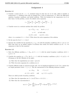
The Airy function can be defined in different ways, and here we take an integral
representation suitable for our asymptotic analysis [4]:
Ai(Оѕ ) =
(2)
where
в€ћ
=
в€ћ
1
в€Є
в€ћ
2
в€Є
в€ћ
3 ,
в€’1
2ПЂi
eв€’Оѕ z+1/3z dz,
3
в€ћ
which are defined as (see Figure 1)
в€ћ
1
= {−teπ i/3 |−∞ < t ≤ −1},
в€ћ
3
= {te5π i/3 |1 ≤ t < ∞}.
в€ћ
2
= e−tπ i |− 13 ≤ t ≤
1
3
,
The breakthrough in the complex category is by [4], which is for any finite rank
spiked model. In the rank 1 case, it is:
P ROPOSITION 2.
In the rank 1 complex spiked model:
1. If в€’1 < a < Оі в€’1 , then the distribution of the largest sample eigenvalue is the
same as that of the complex white Wishart ensemble in Proposition 1.
2. If a = Оі в€’1 , then the limit and the fluctuation scale are the same as those of the
complex white Wishart ensemble, but the distribution function is
(3)
lim P max(О») в€’ (1 + Оі в€’1 )2 В·
M→∞
F IG . 1.
Оі M 2/3
≤T
(1 + Оі )4/3
в€ћ.
= FGUE1 (T ).
1276
D. WANG
3. If a > Оі в€’1 , then the limit and the fluctuation scale are changed as well as the
distribution function, which is a Gaussian:
в€љ
1
M
lim P max(О») в€’ (a + 1) 1 + 2
В·
≤T
M→∞
Оі a
(a + 1) 1 в€’ 1/(Оі 2 a 2 )
(4)
T
1
2
в€љ eв€’t /2 dt.
=
в€’в€ћ 2ПЂ
The function FGUE1 occurring in (3) is defined similarly to FGUE [4]:
(5)
FGUE1 (T ) = det 1 в€’ KAiry (Оѕ, О·) + s (1) (Оѕ ) Ai(О·) П‡(T ,в€ћ) (О·) ,
where s (1) is one of a series of functions defined in [4], and has the integral representation
в€ћ
1
в€’О·z+1/3z3 1
(1)
s (1) (О·) =
dz
and
s
e
(О·)
=
1
в€’
Ai(t) dt,
2ПЂi ВЇВЇ в€ћ
z
О·
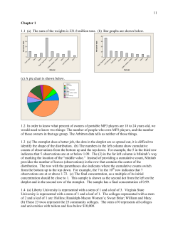
where ВЇВЇ в€ћ = ВЇВЇ в€ћ в€Є ВЇВЇ в€ћ в€Є ВЇВЇ в€ћ , which are defined as (see Figure 2 Оµ is a positive
1
constant, used later)
2
3
¯¯ ∞ = ε etπ i 1 ≤ t ≤ 5 ,
2
2
3
3
¯¯ ∞ = −teπ i/3 −∞ < t ≤ − ε ,
1
2
5ПЂ i/3 Оµ
ВЇВЇ в€ћ
≤t <∞ .
3 = te
2
R EMARK 1. The kernel in (5) is not in trace class, but the Fredholm determinant is well defined and we can easily conjugate it into a trace class kernel. Several
kernels below are in similar situations.
F IG . 2.
ВЇВЇ в€ћ .
1277
QUATERNIONIC WISHART
In the real category, we have the result for the real white Whishart ensemble:
P ROPOSITION 3. The distribution of the largest sample eigenvalue in the real
white Wishart ensemble satisfies that, max(О») almost surely approaches [15] (1 +
Оі в€’1 )2 with fluctuation scale M в€’2/3 , and [19]
lim P max(О») в€’ (1 + Оі в€’1 )2 В·
M→∞
Оі M 2/3
≤T
(1 + Оі )4/3
= FGOE (T ),
where FGOE is the GOE Tracy–Widom distribution.
Here the function FGOE is defined by the Fredholm determinant of a matrix
integral operator [30]:
FGOE (T ) = det I в€’ PGOE (Оѕ, О·)
and
S1 (Оѕ, О·)
SD1 (Оѕ, О·)
П‡(T ,в€ћ) (О·),
1
IS1 (Оѕ, О·) в€’ 2 sgn(x в€’ y) S1 (О·, Оѕ, )
PGOE (Оѕ, О·) = П‡(T ,в€ћ) (Оѕ )
where
S1 (Оѕ, О·) = KAiry (Оѕ, О·) в€’
SD1 (Оѕ, О·) = в€’
в€’
(6)
в€ћ
Ai(t) dt +
О·
1
Ai(Оѕ ),
2
∂
1
KAiry (Оѕ, О·) в€’ Ai(Оѕ ) Ai(О·),
∂η
2
IS1 (Оѕ, О·) = в€’
R EMARK 2.
1
Ai(Оѕ )
2
в€ћ
Оѕ
1
2
KAiry (t, О·) dt +
в€ћ
Оѕ
Ai(t) dt +
1
2
1
2
в€ћ
Оѕ
в€ћ
в€ћ
Ai(t) dt
Ai(t) dt
О·
Ai(t) dt.
О·
We have a more convenient form of FGOE [12]:
FGOE = det 1 в€’ KAiry (Оѕ, О·) + s (1) (Оѕ ) Ai(О·) П‡(T ,в€ћ) (О·) ,
so [4]
FGUE1 (T ) = (FGOE (T ))2 .
In the real spiked model, Baik and Silverstein [8] compute the almost sure limit
of the largest population eigenvalue, which is the same as that in the complex
category, and Paul [25] proves the Gaussian distribution property in the case a >
Оі в€’1 , which is similar to (4). Neither of their methods can find the distribution
function when a ≤ γ −1 .
For the quaternionic white Wishart ensemble, we have:
1278
D. WANG
P ROPOSITION 4. The distribution of the largest sample eigenvalue in the
quaternionic white Wishart ensemble satisfies that, max(О») almost surely approaches (1 + Оі в€’1 )2 with fluctuation scale M в€’2/3 , and [14]
Оі (2M)2/3
≤T
M→∞
(1 + Оі )4/3
where FGSE is the GSE Tracy–Widom distribution.
lim P max(О») в€’ (1 + Оі в€’1 )2 В·
= FGSE (T ),
Here the function FGSE is defined by the Fredholm determinant of a matrix
integral operator [30]:
FGSE (T ) = det I в€’ P (Оѕ, О·)
and
Pˆ (ξ, η) = χ(T ,∞) (ξ )
S4 (Оѕ, О·) SD4 (Оѕ, О·)
П‡(T ,в€ћ) (О·),
IS4 (Оѕ, О·) S4 (О·, Оѕ, )
where
1
1
S4 (Оѕ, О·) = KAiry (Оѕ, О·) в€’ Ai(Оѕ )
2
4
SD4 (Оѕ, О·) = в€’
IS4 (Оѕ, О·) = в€’
в€ћ
Ai(t) dt,
О·
1 ∂
1
KAiry (Оѕ, О·) в€’ Ai(Оѕ ) Ai(О·),
2 ∂η
4
1
2
в€ћ
Оѕ
KAiry (t, О·) dt +
1
4
в€ћ
в€ћ
Ai(t) dt
Оѕ
Ai(t) dt.
О·
1.2. Statement of main results. The main theorem in this paper is:
T HEOREM 1.
In the rank 1 quaternionic spiked model:
1. If в€’1 < a < Оі в€’1 , then the distribution of the largest sample eigenvalue is the
same as that of the quaternionic white Wishart ensemble in Proposition 4.
2. If a = Оі в€’1 , then the limit and the fluctuation scale are the same as those of the
quaternionic white Wishart ensemble, but the distribution function is
lim P
M→∞
max(О») в€’
Оі +1
Оі
2
В·
Оі (2M)2/3
≤T
(1 + Оі )4/3
= FGSE1 (T ).
3. If a > Оі в€’1 , then the limit and the fluctuation scale are changed as well as the
distribution function, which is a Gaussian:
в€љ
2M
1
≤T
В·
lim P max(О») в€’ (a + 1) 1 + 2
M→∞
Оі a
(a + 1) 1 в€’ 1/(Оі 2 a 2 )
=
T
1
2
в€љ eв€’t /2 dt.
в€’в€ћ 2ПЂ
QUATERNIONIC WISHART
1279
Here the function FGSE1 is defined by the Fredholm determinant of a matrix
integral operator:
FGSE1 (T ) = det I в€’ P (Оѕ, О·)
and
P (Оѕ, О·) = П‡(T ,в€ћ) (Оѕ )
S 4 (Оѕ, О·) SD4 (Оѕ, О·)
П‡(T ,в€ћ) (О·),
IS4 (Оѕ, О·) S 4 (О·, Оѕ, )
where
1
Ai(Оѕ ),
SD4 (Оѕ, О·) = SD4 (Оѕ, О·),
2
1 в€ћ
1 в€ћ
IS4 (Оѕ, О·) = IS4 (Оѕ, О·) в€’
Ai(t) dt +
Ai(t) dt.
2 Оѕ
2 О·
S 4 (Оѕ, О·) = S4 (Оѕ, О·) +
Although the distribution FGSE1 seems to be new, we have that
T HEOREM 2.
FGSE1 (T ) = FGOE (T ).
1.3. Relation with other models and conjecture on the rank 1 real spiked
model. The results of Theorems 1 and 2 give a phase transition pattern FGSE –
FGOE –Gaussian as the parameter a increases from −1 to +∞. This pattern appears as limiting distributions indexed by a parameter in several other combinatorial and statistical physical models, for example, the lengths of the longest
monotone subsequences of random involutions with condition on the number of
fixed points [6] and the symmetrized last passage percolation [7] studied by Baik
and Rains. In semi-infinite totally asymmetric simple exclusion process [26] studied by Prähofer and Spohn, and the symmetric polynuclear growth process [5]
studied by Baik et al., 2-dimensional phase transition diagrams are obtained, and
the 1-dimensional FGSE –FGOE –Gaussian pattern is contained in both of them.
Although there is no model which can give hints to the rank 1 real spiked model,
it is plausible that it has a phase transition from FGOE to Gaussian for the limiting
distributions of the largest sample eigenvalue as a goes across Оі в€’1 . Based on the
duality of orthogonal and symplectic models from the Virasoro structure’s point of
view, we have:
C ONJECTURE 1.
In the rank 1 real spiked model:
1. If в€’1 < a < Оі в€’1 , then the distribution of the largest sample eigenvalue is the
same as that of the real white Wishart ensemble in Proposition 3.
1280
D. WANG
2. If a = Оі в€’1 , then the limit and the fluctuation scale are the same as those of the
quaternionic white Wishart ensemble, but the distribution function is
lim P
M→∞
max(О») в€’
Оі +1
Оі
2
В·
Оі (M/2)2/3
≤T
(1 + Оі )4/3
= FGSE (T ).
3. If a > Оі в€’1 , then the limit and the fluctuation scale are changed as well as the
distribution function, which is a Gaussian (proved by Paul in [25]):
в€љ
M/2
1
≤T
В·
lim P max(О») в€’ (a + 1) 1 + 2
M→∞
Оі a
(a + 1) 1 в€’ 1/(Оі 2 a 2 )
=
T
1
2
в€љ eв€’t /2 dt.
в€’в€ћ 2ПЂ
1.4. Structure of the paper. In Section 2 we use combinatorial techniques to
express the joint distribution function of {О»j }, and then by skew orthogonal polynomial techniques express the distribution function of max(О»j ) in the square root
of a Fredholm determinant of a matrix integral operator. In Section 3 we do asymptotic analysis on the kernel of the matrix integral operator, and prove the three
cases of Theorem 1 in the three subsections, respectively. Section 4 contains the
proof of Theorem 2. In the proof of Theorem 1, we use some trace norm convergence results which generalize the old result on the LUE [11], and we give a
method of proof to them in the Appendix.
2. The Fredholm determinantal formula.
2.1. The joint distribution function. In this subsection, we prove the following:
T HEOREM 3. The joint probability distribution function of О» in the quaternionic spiked model is
P (О») =
(7)
N
1 Лњ4
О»j2(Mв€’N)+1 eв€’2MО»j .
V (О»)
C
j =1
In this paper, C stands for any constants, and here
VЛњ 4 (О») =
В·В·В·
В·В·В·
В·В·В·
в€’2
О»2N
1
0
1
2О»1
..
.
в€’3
(2N в€’ 2)О»2N
1
В·В·В·
В·В·В·
О»2Nв€’2
N
0
1
2О»N
..
.
(2N в€’ 2)О»2Nв€’3
N
ea/(1+a)2MО»1
a
a/(1+a)2MО»1
1+a 2Me
В·В·В·
ea/(1+a)2MО»N
a
a/(1+a)2MО»N
1+a 2Me
1
О»1
О»21
..
.
1
О»N
О»2N
..
.
,
1281
QUATERNIONIC WISHART
the determinant of a 2N Г— 2N matrix whose (2N, 2k в€’ 1) entry is ea/(1+a)2MО»k ,
j в€’1
(j, 2k в€’ 1) entry is О»k for j = 1, . . . , 2N в€’ 1, and 2ith column is the derivative
of the (2i в€’ 1)st column. VЛњ 4 (О») is a variation of the V (О»)4 appearing in the LSE
(see [23] and (9)).
For the Wishart ensemble defined in the introduction section, we first have the
distribution function for the sample matrix in the N Г— N positive definite quaternionic Hermitian matrix space [3]:
P (S) =
1 в€’2M
e
C
Tr(
в€’1 S)
(det S)2(Mв€’N)+1 .
R EMARK 3. Due to the noncommutativity of the quaternions, det S is not well
defined in the usual way. Since S is quaternionic Hermitian, we can diagonalize
it into a real-valued diagonal matrix by the conjugation of a quaternionic unitary
matrix U , and define
eigenvalues of U SU в€— .
det S =
N
R EMARK 4. In the distribution function in real and complex categories of
sample matrices, we do not need to take the real part of the trace, since the trace is
already real. Unfortunately, this does not hold in the quaternionic category due to
its noncommutativity, and luckily Tr behaves better. [For example, Tr(AB) =
Tr(BA), but Tr(AB) = Tr(BA) in general.]
The distribution function for sample eigenvalues О», the eigenvalues of S, is
(8)
P (О») =
N
1
(V (О»))4
О»j2(Mв€’N)+1
C
j =1
eв€’2M
Tr(
в€’1 Q
Qв€’1 )
dQ,
Qв€€Sp(N)
where we integrate on the compact symplectic group with the Haar measure,
V (О») = i<j (О»i в€’ О»j ) is the Vandermonde, and = diag(О»1 , . . . , О»N ). (See [23]
for a derivation of the similar GSE case.)
If the perturbation parameter a = 0, then l1 = l2 = В· В· В· = lN = 1,
eв€’2M
Qв€€Sp(N)
Tr(
в€’1 Q
Qв€’1 )
N
dQ =
eв€’2MО»j
j =1
and
(9)
P (О») =
is the standard LSE [23].
N
1
О»j2(Mв€’N)+1 eв€’2MО»j ,
(V (О»))4
C
j =1
1282
D. WANG
Generally,
eв€’2M
Tr(
в€’1 Q
Qв€’1 )
dQ
Qв€€Sp(N)
=
(10)
Tr(I Q Qв€’1 ) в€’2M Tr((
eв€’2M
e
в€’1 в€’I )Q
Qв€’1 )
dQ
Qв€€Sp(N)
N
eв€’2MО»j
=
в€’1 )Q
Tr((I в€’
e2M
Qв€’1 )
dQ.
Qв€€Sp(N)
j =1
Then by the integral formula of the quaternionic Zonal polynomials [17], we get
e2M
Tr((I в€’
в€’1 )Q
Qв€’1 )
dQ
Qв€€Sp(N)
(11)
=
в€ћ
(2M)j
j!
j =0
(1/2)
CОє
в€’1 )C (1/2) (
Оє
(1/2)
CОє (IN )
(I в€’
l(κ)≤N
Оє j
)
,
(1/2)
where CОє (x1 , . . . , xN ) is the N variable quaternionic Zonal polynomial, that is,
the Jack polynomial with the parameter α = 1/2 (see [21] and [27]) and the Cnormalization [10], so that [κ = (k1 , . . . , kl ), k1 ≥ k2 ≥ · · · ≥ kl > 0, then l(κ) = l]
CОє(1/2) (x1 , . . . , xm ) = (x1 + В· В· В· + xm )k .
l(κ)≤m
Оє k
In the formula, a symmetric polynomial of a matrix is equivalent to the symmetric
polynomial of its eigenvalues, so
CОє(1/2) (I в€’
в€’1
) = CОє(1/2)
a
, 0, . . . , 0 .
1+a
(1/2)
Since all variables except for one vanish in CОє
CОє(1/2) (I в€’
(12)
в€’1
(I в€’
в€’1 ),
) l(Оє)>1 = 0.
We have [27]
(1/2)
C(j )
a
a
, 0, . . . , 0 =
1+a
1+a
j
and since the number of variables is N [27]
(1/2)
C(j ) (1, . . . , 1) =
1
(j + 1)!
j в€’1
(2N + i),
i=0
we simply find
1283
QUATERNIONIC WISHART
so with (11) and (12), we get
Tr((I в€’
e2M
в€’1 )Q
Qв€’1 )
dQ
Qв€€Sp(N)
в€’1 )C
(2M)j C(j ) (I в€’
(j ) ( )
=
(1/2)
j!
C(j ) (IN )
j =0
(1/2)
в€ћ
в€ћ
=
(1/2)
j +1
j
a
2M
j в€’1
1+a
i=0 (2N + i)
j =0
(1/2)
C(j ) ( ).
In [27] there is an identity
в€ћ
N
(1/2)
(j + 1)C(j ) ( )t j =
j =0
1
.
(1 в€’ О»j t)2
j =1
Comparing it with the well-known identity for Schur polynomials
в€ћ
N
s(j ) ( )t j =
j =0
1
,
1 в€’ О»j t
j =1
we get the identity
(1/2)
(j + 1)C(j ) ( ) = s(j ) (О»1 , О»1 , О»2 , О»2 , . . . , О»N , О»N ),
(13)
with each О»i appearing twice as variables of the s(j ) . For notational simplicity, we
denote the right-hand side of (13) as sЛњ(j ) ( ), which is a plethysm [21]
sЛњ(j ) ( ) = s(j ) в—¦ 2p1 ( ).
Now we get
e2M
Tr((I в€’
в€’1 )Q
Qв€’1 )
dQ
Qв€€Sp(N)
(14)
в€ћ
=
1
j =0
a
2M
j в€’1
1+a
i=0 (2N + i)
j
sЛњ(j ) ( ).
Then we need a lemma to simplify (14) further.
L EMMA 1.
sЛњ(j ) ( ) =
1
О»1
О»21
..
.
0
1
2О»1
..
.
(2N в€’ 2)О»2Nв€’3
1
О»2Nв€’2
1
(15)
2N+j в€’1
О»1
(2N + j
Г— V (О»)в€’4 ,
2N+j в€’2
в€’ 1)О»1
В·В·В·
В·В·В·
В·В·В·
В·В·В·
В·В·В·
В·В·В·
1
О»N
О»2N
..
.
О»2Nв€’2
N
2N+j в€’1
О»N
0
1
2О»N
..
.
(2N в€’ 2)О»2Nв€’3
N
2N+j в€’2
(2N + j в€’ 1)О»N
1284
D. WANG
with the (k, 2j в€’ 1) entry of the matrix being a power of О»j with the exponent k в€’ 1
if k = 2N and 2N + j в€’ 1 if k = 2N , and the (k, 2j ) entry being the derivative of
the (k, 2j в€’ 1) entry with respect to О»j .
To prove this lemma, we need the well-known fact (see [23]), proven by
L’Hôpital’s rule
0
1
..
.
О»12Nв€’1
(2N в€’ 1)О»12Nв€’2
V (О»)4 =
(16)
В·В·В·
В·В·В·
1
О»1
..
.
1
О»N
..
.
0
1
..
.
В·В·В·
2Nв€’1
В· В· В· О»N
,
2Nв€’2
(2N в€’ 1)О»N
with the (k, 2j в€’ 1) entry being О»kв€’1
and the (k, 2j ) entry (k в€’ 1)О»kв€’2
j
j .
P ROOF OF L EMMA 1. Applying the L’Hôpital’s rule repeatedly with respect
to x2i , i = 1, . . . , N , we get the identity
1
О»1
0
1
В·В·В·
В·В·В·
1
О»N
0
1
О»21
.
.
.
2О»1
.
.
.
В·В·В·
В·В·В·
О»2N
.
.
.
2О»N
.
.
.
в€’2
О»2N
1
в€’3
(2N в€’ 2)О»2N
1
В·В·В·
в€’2
О»2N
N
в€’3
(2N в€’ 2)О»2N
N
В·В·В·
2N +j в€’1
О»N
2N +j в€’1
О»1
(2N + j
2N +j в€’2
в€’ 1)О»1
1
О»1
.
.
.
0
1
.
.
.
В·В·В·
В·В·В·
в€’1
О»2N
1
(2N в€’ 1)О»2N в€’2
вЋ›
2N +j в€’2
(2N + j в€’ 1)О»N
В·В·В·
1
О»N
.
.
.
0
1
.
.
.
В·В·В·
в€’1
О»2N
N
в€’2
(2N в€’ 1)О»2N
N
1
x1
.
.
.
1
x2
.
.
.
В·В·В·
В·В·В·
x12N в€’2
x22N в€’2
2N +j в€’1
x1
2N +j в€’1
x2
1
x1
.
.
.
1
x2
.
.
.
В·В·В·
В·В·В·
x12N в€’2
x22N в€’2
2N +j в€’1
x1
2N +j в€’1
x2
вЋњ
∂N
вЋњ
⎝ ∂x2 ∂x4 · · · ∂x2N
=вЋњ
∂N
∂x2 ∂x4 · · · ∂x2N
В·В·В·
1
x2N в€’1
.
.
.
1
x2N
.
.
.
В·В·В·
2N в€’2
x2N
в€’1
2N в€’2
x2N
В·В·В·
2N +j в€’1
x2N в€’1
2N +j в€’1
x2N
вЋћ
В·В·В·
1
x2N в€’1
.
.
.
1
x2N
.
.
.
В·В·В·
2N в€’2
x2N
в€’1
2N в€’2
x2N
В·В·В·
2N +j в€’1
x2N в€’1
вЋџ
вЋџ
вЋџ
вЋџ
вЋџ
вЋџ
вЋџ
вЋџ
вЋ 2N +j в€’1
x2N
x2iв€’1 = x2i = О»i
i = 1, . . . , N
= s(j ) (О»1 , О»1 , О»2 , О»2 , . . . , О»N , О»N ) = sЛњ(j ) ( ),
from the matrix representation of Schur polynomials, and now use (16) to get the
compact formula (15).
1285
QUATERNIONIC WISHART
Substituting (15) into (14), we get
V (О»)4
Tr((I в€’
e2M
в€’1 )Q
Qв€’1 )
dQ
Qв€€Sp(N)
1
О»1
0
1
В·В·В·
В·В·В·
1
О»N
0
1
О»21
.
.
.
2О»1
.
.
.
В·В·В·
В·В·В·
О»2N
.
.
.
2О»N
.
.
.
в€’2
О»2N
1
в€’3
(2N в€’ 2)О»2N
1
В·В·В·
в€’2
О»2N
N
в€’3
(2N в€’ 2)О»2N
N
p(О»1 )
p (О»1 )
=
(17)
=
=
1
C
В· В· В· p(О»N )
p (О»N )
1
О»1
0
1
В·В·В·
В·В·В·
1
О»N
0
1
О»21
.
.
.
2О»1
.
.
.
В·В·В·
В·В·В·
О»2N
.
.
.
2О»N
.
.
.
в€’2
О»2N
1
в€’3
(2N в€’ 2)О»2N
1
В·В·В·
ea/(1+a)2MО»1
a
a/(1+a)2MО»1
1+a 2Me
В·В·В·
в€’2
О»2N
N
a/(1+a)2MО»
N
e
в€’3
(2N в€’ 2)О»2N
N
a
a/(1+a)2MО»
N
1+a 2Me
1 Лњ4
V (О»),
C
where
в€ћ
p(x) =
j =0
=
1
a
2M
j в€’1
1+a
i=0 (2N + i)
j
x 2N+j в€’1
2Nв€’2
(2N в€’ 1)!
1
a
a/(1+a)2Mx
e
в€’
2Mx
2Nв€’1
(a/(1 + a)2M)
j! 1 + a
j =0
j
,
and if k = 2N , the (k, 2j в€’ 1) entries in both matrices are О»kв€’1
j , and the (k, 2j )
kв€’2
entries are (k в€’ 1)О»j , and the 2N, 2i в€’ 1 entry in the former (latter) matrix is
p(О»i ) (resp. ea/(1+a)2MО»i ) and the 2N, 2i entry p (О»i ) (resp.
P ROOF
sult (7).
OF
T HEOREM 3.
a
a/(1+a)2MО»i ).
1+a 2Me
Formulas (8), (10) and (17) together give the re-
2.2. The Pfaffian and determinantal formulas. With the formula (7) ready to
use, we apply the standard RMT technique to get the distribution formula for the
largest sample eigenvalue, in the same spirit as the solution of the LSE. Our process
below is closely parallel to that in [31] to the LSE.
First, we find a skew orthogonal basis {П•0 (x), П•1 (x), . . . , П•2Nв€’1 (x)} of the linear space spanned by {1, x, x 2 , . . . , x 2Nв€’2 , ea/(1+a)2Mx }. We require that the П•j (x)
is a linear combination of {1, x, x 2 , . . . , x j } if j < 2N в€’ 1, while П•2Nв€’1 (x) can be
1286
D. WANG
arbitrary, with the skew inner products among them
П•j (x), П•k (x)
4
в€ћ
=
=
0
П•j (x)П•k (x) в€’ П•j (x)П•k (x) x 2(Mв€’N)+1 eв€’2Mx dx
вЋ§
вЋЁ rj/2 ,
вЋ©
в€’rk/2 ,
0,
if j is even and k = j + 1,
if k is even and j = k + 1,
otherwise.
Then we can reformulate the distribution function of О» as
P (О») =
П•0 (О»1 )
П•1 (О»1 )
..
.
П•0 (О»1 )
П•1 (О»1 )
..
.
П•2Nв€’1 (О»1 )
П•2Nв€’1 (О»1 )
1
C
N
Г—
(18)
j =1
=
П•0 (О»N )
П•1 (О»N )
..
.
П•0 (О»N )
П•1 (О»N )
..
.
В·В·В·
В· В· В· П•2Nв€’1 (О»N ) П•2Nв€’1 (О»N )
О»j2(Mв€’N)+1 eв€’2MО»j
П€0 (О»1 )
П€1 (О»1 )
..
.
1
C
В·В·В·
В·В·В·
П€2Nв€’1 (О»1 )
П€0 (О»1 )
П€1 (О»1 )
..
.
В·В·В·
В·В·В·
П€0 (О»N )
П€1 (О»N )
..
.
В·В·В·
П€2Nв€’1 (О»1 ) В· В· В· П€2Nв€’1 (О»N )
П€0 (О»N )
П€1 (О»N )
..
.
,
П€2Nв€’1 (О»N )
where
П€i (x) = П•i (x)x Mв€’N+1/2 eв€’Mx .
(19)
For an arbitrary function f (x) on [0, в€ћ), by the formula of de Bruijn [9],
в€ћ
0
В·В·В·
П€0 (О»1 )
П€1 (О»1 )
..
.
П€0 (О»1 )
П€1 (О»1 )
..
.
П€2Nв€’1 (О»1 )
П€2Nв€’1 (О»1 )
в€ћ
0
(20)
В·В·В·
В·В·В·
П€0 (О»N )
П€1 (О»N )
..
.
В·В·В·
В· В· В· П€2Nв€’1 (О»N )
П€0 (О»N )
П€1 (О»N )
..
.
П€2Nв€’1 (О»N )
N
Г—
1 + f (О»i ) dО»i = C Pf P (1 + f ) ,
i=1
where P (1 + f ) is a 2N Г— 2N matrix, whose entries depend on 1 + f in the
following way:
P (1 + f )
j,k
=
в€ћ
0
П€j в€’1 (x)П€kв€’1 (x) в€’ П€j в€’1 (x)П€kв€’1 (x) 1 + f (x) dx.
1287
QUATERNIONIC WISHART
Now we define a matrix Z as
вЋ›
0
вЋњ в€’r0
вЋњ
вЋћ
r0
0
вЋњ
вЋњ
вЋњ
Z=вЋњ
вЋњ
вЋњ
вЋњ
вЋќ
0
в€’r1
r1
0
..
.
0
в€’rNв€’1
with
вЋ§
вЋЁ rk/2в€’1 ,
Zj,k =
,
в€’r
вЋ© j/2в€’1
0,
rNв€’1
0
вЋџ
вЋџ
вЋџ
вЋџ
вЋџ
вЋџ,
вЋџ
вЋџ
вЋџ
вЋ if k is even and j = k в€’ 1,
if j is even and k = j в€’ 1,
otherwise,
and define for j = 0, . . . , N в€’ 1, О· = Z в€’1 П€, that is,
О·2j (x) = в€’
П€2j +1 (x)
rj
and
О·2j +1 (x) =
П€2j (x)
.
rj
So we have
P (1 + f )
j,k =
в€ћ
0
+
П€j в€’1 (x)П€kв€’1 (x) в€’ П€j в€’1 (x)П€kв€’1 (x) dx
в€ћ
0
П€j в€’1 (x)П€kв€’1 (x) в€’ П€j в€’1 (x)П€kв€’1 (x) f (x) dx
в€ћ
= Zj,k +
0
П€j в€’1 (x)П€kв€’1 (x) в€’ П€j в€’1 (x)П€kв€’1 (x) f (x) dx.
And if we denote Q(1 + f ) = Z в€’1 P (1 + f ), then
Q(1 + f )j,k = Оґj,k +
в€ћ
0
О·j в€’1 (x)П€kв€’1 (x) в€’ О·j в€’1 (x)П€kв€’1 (x) f (x) dx.
If we choose f to be в€’П‡(T ,в€ћ) , then the integral on the left-hand side of (20),
after multiplying a constant, is the probability of all λi ’s smaller than T . In latter part of the paper, we abbreviate χ(T ,∞) to χ . So we get for a T -independent
constant
P max(λi ) ≤ T = C Pf P (1 − χ ) ,
and
P max(λi ) ≤ T
2
= C 2 det P (1 в€’ П‡ ) = C 2 det Q(1 в€’ П‡ ) .
In linear algebra, we have the determinant identity
(21)
det(I в€’ AB) = det(I в€’ BA),
1288
D. WANG
for A an m Г— n matrix and B an n Г— m matrix, but the identity still holds in infinite
dimensional settings [16]. Letting det mean a Fredholm determinant for matrix
integral operators, we describe a setting due to Tracy–Widom [31].
If A is an operator from L2 ([0, в€ћ)) Г— L2 ([0, в€ћ)) to the vector space R2N with
A
g(x)
h(x)
j
=
в€ћ
0
П‡ (x)О·j в€’1 (x)g(x) dx в€’
в€ћ
0
П‡ (x)О·j в€’1 (x)h(x) dx,
and B is an operator from R2N to L2 ([0, в€ћ)) Г— L2 ([0, в€ћ)) with
вЋ›
вЋћ
вЋ› 2N
вЋћ
ck П€kв€’1 (x)П‡(x) вЋџ
c1
вЋњ
вЋџ
вЋњ .. вЋџ вЋњ
k=1
вЋњ
вЋџ,
B вЋќ . вЋ = вЋњ 2N
вЋџ
вЋќ
вЋ c2N
ck П€kв€’1 (x)П‡(x)
k=1
then
I в€’ AB = Q(1 в€’ П‡ )
and
I в€’ BA = I в€’ П‡ (x)
S4 (x, y) SD4 (x, y)
П‡ (y),
IS4 (x, y) S4 (y, x)
where S4 (x, y), IS4 (x, y) and SD4 (x, y) are integral operators whose kernels are
2Nв€’1
S4 (x, y) =
П€j (x)О·j (y)
j =0
Nв€’1
=
j =0
1
в€’П€2j (x)П€2j +1 (y) + П€2j +1 (x)П€2j (y) ,
rj
2Nв€’1
SD4 (x, y) =
в€’П€j (x)О·j (y)
j =0
(22)
Nв€’1
=
j =0
1
П€ (x)П€2j +1 (y) в€’ П€2j +1 (x)П€2j (y) ,
rj 2j
2Nв€’1
IS4 (x, y) =
П€j (x)О·j (y)
j =0
Nв€’1
=
j =0
1
в€’П€2j (x)П€2j +1 (y) + П€2j +1 (x)П€2j (y) ,
rj
QUATERNIONIC WISHART
1289
2Nв€’1
S4 (y, x) =
j =0
(23)
Nв€’1
=
j =0
в€’П€j (x)О·j (y)
1
П€2j (x)П€2j +1 (y) в€’ П€2j +1 (x)П€2j (y) .
rj
R EMARK 5. It is clear that the nomenclature of SD4 (x, y) is due to the fact
that SD4 (x, y) is the negative of the derivative of S4 (x, y). But IS4 (x, y), which
gets its name in the same way in earlier literature in GSE (e.g., [30]), in our problem may not satisfy the equation
IS4 (x, y) = в€’
в€ћ
x
S4 (t, y) dt,
since the integral on the right-hand side may diverge.
In conclusion,
P max(λi ) ≤ T
2
= C 2 det I в€’ П‡ (x)
S4 (x, y) SD4 (x, y)
П‡ (y) ,
IS4 (x, y) S4 (y, x)
and we can find that C 2 = 1 by taking the limit T в†’ в€ћ. We define a 2 Г— 2 matrix
kernel as
PT (x, y) = П‡ (x)
=
S4 (x, y) SD4 (x, y)
П‡ (y)
IS4 (x, y) S4 (y, x)
П‡ (x)S4 (x, y)П‡(y) П‡(x)DS4 (x, y)П‡(y)
,
П‡ (x)IS4 (x, y)П‡(y) П‡(x)S4 (y, x)П‡(y)
then we have
P max(λi ) ≤ T
2
= det I в€’ PT (x, y) .
2.3. S4 (x, y) in terms of Laguerre polynomials. In manipulation of skew orthogonal polynomials, we take the approach of [1], and all classical orthogonal
polynomial properties are from [28].
Since Laguerre polynomials by definition satisfy the orthogonal property
в€ћ
0
(О±) О± в€’x
L(О±)
dx =
j Lk x e
(j + О±)!
Оґj,k ,
j!
(О±)
and they have the differential identity [we assume Ln (x) = 0 if n < 0]
(24)
x
d (О±)
(О±)
L (x) = nL(О±)
n (x) в€’ (n + О±)Lnв€’1 (x),
dx n
1290
D. WANG
it is easy to get that
L(2(Mв€’N))
(2Mx), L(2(Mв€’N))
(2Mx) 4
j
k
=
в€ћ
0
d (2(Mв€’N))
L
(2Mx)
dx k
d (2(Mв€’N))
(2(Mв€’N))
в€’ Lk
(2Mx) Lj
(2Mx)
dx
(2(Mв€’N))
Lj
(2Mx)
Г— x 2(Mв€’N)+1 eв€’2Mx dx
=
вЋ§
вЋЄ
1 2(Mв€’N)+1 (j + 2(M в€’ N))!
вЋЄ
вЋЄ
,
вЋЄ
вЋЄ
вЋЁ 2M
(j в€’ 1)!
if j = k + 1,
1
вЋЄ
вЋЄ
в€’
вЋЄ
вЋЄ
вЋЄ
2M
вЋ©
if k = j + 1,
2(Mв€’N)+1
0,
(k + 2(M в€’ N))!
,
(k в€’ 1)!
otherwise.
So we can choose for j = 0, . . . , N в€’ 2,
j
k
П•2j (x) =
(25)
k=0
2i в€’ 1
(2(Mв€’N))
L2k
(2Mx),
2i
+
2(M
в€’
N)
i=1
(2(Mв€’N))
П•2j +1 (x) = в€’L2j +1
(26)
(2Mx)
and
(27)
rj =
1
2M
2(Mв€’N)+1
j
(2j + 2(M в€’ N) + 1)!
2k в€’ 1
.
(2j )!
2k + 2(M в€’ N)
k=1
We can also choose
Nв€’1
П•2Nв€’2 (x) =
k=0
k
2i в€’ 1
L(2(Mв€’N))
(2Mx),
2k
2i
+
2(M
в€’
N)
i=1
but П•2Nв€’1 (x) is not a polynomial and needs to be treated separately.
By the Rodrigues’ representation
1 d n в€’x n+О±
(e x
),
n! dx n
and repeated integration by parts, we get for n > 0
x О± eв€’x L(О±)
n (x) =
ea/(1+a)2Mx , L(2(Mв€’N))
(2Mx) 4
n
=
1+a
2M
2(Mв€’N)+1
(n + 2(M в€’ N) + 1)!
n!
(n + 2(M в€’ N))!
в€’ (в€’a)nв€’1
(n в€’ 1)!
(в€’a)n+1
1291
QUATERNIONIC WISHART
and
ea/(1+a)2Mx , L(2(Mв€’N))
(2Mx) 4 = в€’
0
1+a
2M
2(Mв€’N)+1
a 2(M в€’ N) + 1 !,
so that
ea/(1+a)2Mx , П•2j (x) 4
=в€’
1+a
2M
2(Mв€’N)+1
a 2j +1
j
(2j + 2(M в€’ N) + 1)!
2k в€’ 1
(2j )!
2k + 2(M в€’ N)
k=1
and
ea/(1+a)2Mx , П•2j +1 (x) 4
=в€’
1+a
2M
2(Mв€’N)+1
a 2j +2
(2j + 2(M в€’ N) + 2)!
(2j + 1)!
(2j + 2(M в€’ N) + 1)!
.
(2j )!
Now by the skew orthogonality, we can choose
в€’ a 2j
Nв€’2
П•2Nв€’1 (x) = ea/(1+a)2Mx в€’
j =0
1 a/(1+a)2Mx
e
, П•2j +1 (x) 4 П•2j (x)
rj
в€’ ea/(1+a)2Mx , П•2j (x) 4 П•2j +1 (x)
Nв€’1
в€’ (1 + a)2(Mв€’N)+1 a 2Nв€’2
j =1
2j + 2(M в€’ N)
П•2Nв€’2 (x)
2j в€’ 1
2Nв€’2
=e
a/(1+a)2Mx
в€’ (1 + a)
2(Mв€’N)+1
j =0
(2(Mв€’N))
(в€’a)j Lj
(2Mx)
and
rNв€’1 =
1+a
2M
2(Mв€’N)+1
a 2Nв€’1
(2M в€’ 1)! Nв€’1
2k в€’ 1
.
(2N в€’ 2)! k=1 2k + 2(M в€’ N)
Now, we write S4 (x, y) as S4a (x, y) + S4b (x, y), where
Nв€’2
(28)
S4a (x, y) =
j =0
1
в€’П€2j (x)П€2j +1 (y) + П€2j +1 (x)П€2j (y)
rj
and
S4b (x, y) =
1
в€’П€2Nв€’2 (x)П€2Nв€’1 (y) + П€2Nв€’1 (x)П€2Nв€’2 (y) ,
rNв€’1
and simplify them separately.
(29)
1292
D. WANG
The formula (28) of our S4a (x, y) is also the formula for S4 (x, y) in the LSE
problem, with parameters M and N в€’ 2, and has been well studied. For completeness we derive its Laguerre polynomial expression here, following [1].
By the differential identity (24) and the identity
(О±)
(О±)
nL(О±)
n (x) = (в€’x + 2n + О± в€’ 1)Lnв€’1 (x) в€’ (n + О± в€’ 1)Lnв€’2 (x),
we get, remembering the definition (19), the telescoping sequence
j
k
2i в€’ 1
2i + 2(M в€’ N)
i=1
П€2j (x) =
k=0
Г— M в€’ N + 1/2 в€’ Mx + x
d
(2(Mв€’N))
L2k
(2Mx)
dx
Г— x Mв€’Nв€’1/2 eв€’Mx
j
=
(30)
k
2i в€’ 1
1
(2(Mв€’N))
(2k + 1)L2k+1
(2Mx)
2 k=0 i=1 2i + 2(M в€’ N)
(2(Mв€’N))
в€’ 2k + 2(M в€’ N) L2kв€’1
(2Mx)
Г— x Mв€’Nв€’1/2 eв€’Mx
=
1
2
j
2k в€’ 1
2k + 2(M в€’ N)
k=1
Г— (2j + 1)L(2(Mв€’N))
(2Mx)x Mв€’Nв€’1/2 eв€’Mx
2j +1
and
П€2j +1 (x) = в€’ M в€’ N + 1/2 в€’ Mx + x
d
(2(Mв€’N))
L
dx 2j +1
Г— (2Mx)x Mв€’Nв€’1/2 eв€’Mx
1
(2(Mв€’N))
= в€’ (2j + 2)L2j +2
(2Mx)
2
(31)
(2(Mв€’N))
в€’ 2j + 2(M в€’ N) + 1 L2j
(2Mx)
Г— x Mв€’Nв€’1/2 eв€’Mx .
Therefore, if we substitute (27), (30) and (31) into (28), we get after some trick,
1
S4a (x, y) = (2M)2(Mв€’N)+1 x Mв€’Nв€’1/2 eв€’Mx y Mв€’N+1/2 eв€’My
2
2Nв€’2
Г—
j =0
j!
(2(Mв€’N))
(2(Mв€’N))
Lj
(2Mx)Lj
(2My)
(j + 2(M в€’ N))!
QUATERNIONIC WISHART
в€’
(2N в€’ 2)!
(2M в€’ 2)!
Nв€’1
j =1
1293
2j + 2(M в€’ N)
2j в€’ 1
Г— L(2(Mв€’N))
(2Mx)П•2Nв€’2 (y) .
2Nв€’2
Furthermore, we can simplify П€2Nв€’2 (x). Since for j = 2N в€’ 1 [if we define
П•j (x) and then П€j (x) for j > 2N в€’ 1 by the formula (25) and (26)]
в€ћ
0
П€2Nв€’2 (x)П€j (x) в€’ П€2Nв€’2 (x)П€j (x) dx = 0,
we get for j = 2N в€’ 1, using integration by parts,
в€ћ
0
(2(Mв€’N))
П€2Nв€’2 (x)Lj
(2Mx)x Mв€’N+1/2 eв€’Mx dx = 0.
So by the orthogonal property of Laguerre polynomials, we get
П€2Nв€’2 (x) = CL(2(Mв€’N))
(2Mx)x Mв€’Nв€’1/2 eв€’Mx ,
2Nв€’1
and we can determine that
2j в€’ 1
2N в€’ 1 Nв€’1
2
2j + 2(M в€’ N)
j =1
C=
without much difficulty. Together with the fact limx→∞ ψ2N−2 (x) = 0, we get
П€2Nв€’2 (x) = в€’
2j в€’ 1
2N в€’ 1 Nв€’1
2
2j + 2(M в€’ N)
j =1
Г—
в€ћ
x
t Mв€’Nв€’1/2 eв€’Mt L(2(Mв€’N))
(2Mt) dt.
2Nв€’1
Now, we can write S4a (x, y) as S4a1 (x, y) + S4a2 (x, y), where
1
S4a1 (x, y) = (2M)2(Mв€’N)+1
2
2Nв€’2
(32)
Г—
j =0
j!
(2(Mв€’N))
Lj
(2Mx)x Mв€’Nв€’1/2 eв€’Mx
(j + 2(M в€’ N))!
(2My)y Mв€’N+1/2 eв€’My
Г— L(2(Mв€’N))
j
and
1
(2N в€’ 1)!
S4a2 (x, y) = (2M)2(Mв€’N)+1
4
(2M в€’ 2)!
(33)
(2(Mв€’N))
Г— L2Nв€’2
Г—
в€ћ
y
(2Mx)x Mв€’Nв€’1/2 eв€’Mx
t Mв€’Nв€’1/2 eв€’Mt L(2(Mв€’N))
(2Mt) dt.
2Nв€’1
1294
D. WANG
Finally,
S4b (x, y) = в€’
1 2M
2 1+a
2(Mв€’N)+1
(2(Mв€’N))
Г— L2Nв€’1
(34)
a в€’(2Nв€’1)
(2N в€’ 1)!
(2M в€’ 1)!
(2Mx)x Mв€’Nв€’1/2 eв€’Mx П€2Nв€’1 (y)
+ П€2Nв€’1 (x)
в€ћ
y
(2(Mв€’N))
L2Nв€’1
(2Mt)t Mв€’Nв€’1/2 eв€’Mt dt ,
and we can take the asymptotic analyses of S4a1 (x, y), S4a2 (x, y) and S4b (x, y)
separately.
3. Asymptotic analysis. In order to consider the rescaled distribution problem, we wish to find the probability of the largest sample eigenvalue being in the
domain (0, p + qT ]. We can put the kernel in the new coordinate system [after a
conjugation by
q 1/2
0
0
q в€’1/2
P max(λi ) ≤ p + qT
], and get
2
S4 (Оѕ, О·) SD4 (Оѕ, О·)
П‡ (О·)
IS4 (Оѕ, О·) S4 (О·, Оѕ )
= det I в€’ П‡ (x)
= det I в€’ PT (Оѕ, О·) ,
where as L2 functions,
SD4 (Оѕ, О·) = q 2 SD4 (x, y)|x=p+qОѕ ,
(35)
y=p+qО·
S4 (Оѕ, О·) = qS4 (x, y)|x=p+qОѕ ,
(36)
y=p+qО·
IS4 (Оѕ О·) = IS4 (x, y)|x=p+qОѕ
(37)
y=p+qО·
and
PT (Оѕ, О·) = П‡ (Оѕ )
S4 (Оѕ, О·) SD4 (Оѕ, О·)
П‡ (О·).
IS4 (Оѕ, О·) S4 (О·, Оѕ )
In this section, we want to prove that for fixed γ ≥ 1 and a > −1, we can choose
suitable pM and qM depending on M, so that for any T ,
lim P max(λi ) ≤ pM + qM T
M→∞
2
= lim det I в€’ PT (Оѕ, О·) = fa (T ),
M→∞
where fa is a function to be determined.
To prove the convergence of Fredholm determinants, we may use that PT (Оѕ, О·)
is in trace class for any M and converges to a certain 2 Г— 2 matrix kernel in trace
norm. Equivalently, we may use that each entry of PT (Оѕ, О·) is in trace class and
converges to a scalar kernel in trace norm. It turns out later that the PT (ξ, η)’s may
not satisfy these requirements, but certain conjugates do.
1295
QUATERNIONIC WISHART
Since the IS4 (x, y) and DS4 (x, y) are of the same form as S4 (x, y), we only
show the asymptotic analysis of S4 (x, y), and state the result for the other two, for
which the arguments are the same.
3.1. Proof of the −1 < a < γ −1 part of Theorem 1. In case −1 < a ≤ γ −1 ,
)4/3
, and denote [here в€— stands for 4,
we choose pM = (1 + Оі в€’1 )2 and qM = Оі(1+Оі
(2M)2/3
4a, 4a1, 4a2 and 4b; the definition of Sв€— (Оѕ, О·) in (38) is only used in Sections 3.1
and 3.2]
(38)
Sв€— (Оѕ, О·) =
(1 + Оі )4/3
Sв€— (x, y)|x=(1+Оі в€’1 )2 +(1+Оі )4/3 /(Оі (2M)2/3 )Оѕ .
Оі (2M)2/3
y=(1+Оі в€’1 )2 +(1+Оі )4/3 /(Оі (2M)2/3 )О·
S4a (x, y) is the formula for the upper-left entry of the 2 Г— 2 matrix kernel of the
LSE problem with parameters M and N в€’ 1, and its asymptotic behavior is well
studied [14]. We want to prove that as M в†’ в€ћ, S4a (x, y) dominates S4 (x, y) in
the domain that we are interested in, and so naturally the distribution of the largest
sample eigenvalue in the perturbed problem is the same as that in the LSE problem.
(The difference between N and N в€’ 1 is negligible.)
S4a1 (x, y) is almost the kernel for
в€љ the LUE problem with parameters
2M в€’ 2 and 2N в€’ 2, besides a factor y/x/2. From a standard result for LUE
[11], П‡T (Оѕ )S4a1 (Оѕ, О·)П‡T (О·) is in trace class and converges in trace norm to half of
the Airy kernel
1
lim П‡ (Оѕ )S4a1 (Оѕ, О·)П‡(О·) = П‡ (Оѕ )KAiry (Оѕ, О·)П‡(О·).
2
More discussion see the Appendix.
For the S4a2 (x, y) part, we also have in trace norm [14],
(39)
(40)
M→∞
1
lim П‡ (Оѕ )S4a2 (Оѕ, О·)П‡(О·) = в€’ П‡ (Оѕ ) Ai(Оѕ )
M→∞
4
в€ћ
Ai(t) dt П‡(О·).
О·
We just sketch the proof. Since S4a2 (Оѕ, О·) is a rank 1 operator, for the trace norm
convergence, we only need to prove that in L2 norm as functions in Оѕ and respectively О·,
lim Оі в€’2N (1 + Оі )4/3 (2M)1/3 eMв€’N
M→∞
(2(Mв€’N))
Г— L2Nв€’2
(41)
(2Mx)x Mв€’Nв€’1/2 eв€’Mx П‡ (Оѕ )
= Ai(Оѕ )П‡(Оѕ ),
в€ћ
lim Оі в€’2N 2MeMв€’N
M→∞
y
(42)
=в€’
в€ћ
О·
L(2(Mв€’N))
(2Mt)t Mв€’Nв€’1/2 eв€’Mt dt П‡(О·)
2Nв€’1
Ai(t) dt П‡(О·)
1296
D. WANG
and by the Stirling’s formula,
lim (2M)2(Mв€’N)в€’1
M→∞
(2N в€’ 1)! 2(Nв€’M) 4Nв€’1
e
Оі
= 1.
(2M в€’ 2)!
By (33), (38), (41) and (42), we get
(2N в€’ 1)! 2(Nв€’M) 4Nв€’1 в€’2N
1
e
П‡ (Оѕ )S4a2 (Оѕ, О·)П‡(О·) = (2M)2(Mв€’N)в€’1
Оі
Оі
4
(2M в€’ 2)!
Г— (1 + Оі )4/3 (2M)1/3 eMв€’N L(2(Mв€’N))
(2Mx)
2Nв€’2
Г— x Mв€’Nв€’1/2 eв€’Mx П‡ (Оѕ )Оі в€’2N 2MeMв€’N
Г—
в€ћ
y
(2(Mв€’N))
L2Nв€’1
(2Mt)t Mв€’Nв€’1/2 eв€’Mt dt П‡(О·).
Therefore we get the trace norm convergence from the L2 convergence by the fact
that if fn (x) в†’ f (x) and gn (y) в†’ g(y) in L2 norm, then we have the convergence
of integral operators in trace norm:
fn (x)gn (y) в†’ f (x)g(y).
Finally, we need to analyze the term S4b (Оѕ, О·), new to the perturbed problem.
We need the following results:
P ROPOSITION 5. For fixed γ ≥ 1 and −1 < a < γ −1 and any T , we have the
convergences in L2 norm with respect to Оѕ or О·:
lim Оі в€’2Nв€’1 (1 + Оі )4/3 (2M)1/3 eMв€’N
M→∞
(2(Mв€’N))
Г— L2Nв€’1
(2Mx)x Mв€’Nв€’1/2 eв€’Mx П‡ (Оѕ )
= в€’ Ai(Оѕ )П‡(Оѕ ),
в€ћ
lim Оі в€’2N 2MeMв€’N
M→∞
=в€’
y
в€ћ
(2(Mв€’N))
L2Nв€’1
Ai(t) dt П‡(О·),
О·
lim (1 + a)2(Nв€’M)в€’1 a в€’2N+1
(43)
(2Mt)t Mв€’Nв€’1/2 eв€’Mt dt П‡(О·)
M→∞
(1 в€’ aОі )(2M)1/3 Mв€’N
e
П€2Nв€’1 (y)П‡(О·)
(Оі + 1)2/3 Оі 2Nв€’1
= Ai(О·)П‡(О·),
lim (1 + a)2(Nв€’M)в€’1 a в€’2N+1
M→∞
= Ai (Оѕ )П‡(Оѕ ).
(1 в€’ aОі )(Оі + 1)2/3 Mв€’N
e
П€2Nв€’1 (x)П‡(Оѕ )
Оі 2N (2M)1/3
1297
QUATERNIONIC WISHART
P ROOF. We just prove the identity (43), and others can be done in the same
way.
By the integral representation of Laguerre polynomials,
eв€’2Mxz (z + 1)n+2(Mв€’N)
1
dz,
2ПЂi C
zn+1
where C is a contour around the pole 0, therefore we get
L(2(Mв€’N))
(2Mx) =
n
(44)
П•2Nв€’1 (y) = ea/(1+a)2My
в€’
(1 + a)2(Mв€’N)+1
2ПЂi
Г—
(45)
eв€’2Myz
C
= ea/(1+a)2My в€’
в€’
(1 + a)2(Mв€’N)
2ПЂi
eв€’2Myz
C
(z + 1)2(Mв€’N)
dz
z + a/(a + 1)
(1 + a)2(Mв€’N)+1 a 2Nв€’1
2ПЂi
Г—
If the pole
1 + (a(z + 1)/z)2Nв€’1 (z + 1)2(Mв€’N)
dz
1 + a(z + 1)/z
z
a
z = в€’ a+1
eв€’2Myz
C
(z + 1)2M
z
dz.
2N
z
((a + 1)z + a)(z + 1)
is inside of C, then
(1 + a)2(Mв€’N)
2ПЂi
eв€’2Myz
C
(z + 1)2(Mв€’N)
dz = ea/(a+1)2My
z + a/(a + 1)
and
П•2Nв€’1 (y) = в€’
(46)
(1 + a)2(Mв€’N)+1 a 2Nв€’1
2ПЂi
Г—
eв€’2Myz
C
(z + 1)2M
z
dz.
2N
z
((a + 1)z + a)(z + 1)
In later part of the proof, we make this condition hold, and will not mention the
canceled terms, and we are then free to deform C in (46) as we wish, provided it
includes 0. We then proceed to a stationary phase analysis.
Since
4/3
(z + 1)2M
2M(в€’(1+Оі в€’1 )2 z+log(z+1)в€’Оі в€’2 log z)в€’ (1+ОіОі) (2M)1/3 О·z
=
e
z2N
(we do not need to concern ourselves about the ambiguity of the value of logarithmic functions), if we denote
eв€’2Myz
(47)
f (z) = в€’(1 + Оі в€’1 )2 z + log(z + 1) в€’ Оі в€’2 log z,
1298
D. WANG
then we get:
в€’1
в€’1 )
)z+Оі
• f (z) = − ((1+γz(z+1)
1
) = 0;
• f (− γ +1
1
• f (− γ +1
)=
2(Оі +1)4
Оі3
1
, with the zero point z = в€’ Оі +1
;
> 0.
1
,
So locally around z = в€’ Оі +1
f в€’
(48)
1
Оі +1
+w =
+ log Оі в€’ (1 в€’ Оі в€’2 ) log(Оі + 1) + Оі в€’2 ПЂi
Оі +1
Оі2
+
(Оі + 1)4 3
w + R1 (w),
3Оі 3
where
R1 (w) = O(w4 ),
(49)
After the substitution w = z +
e2M(в€’yz+log(zв€’1)в€’Оі
в€’2 log z)
C
=
M
exp 2M
=в€’
we get
z
dz
((a + 1)z + a)(z + 1)
Оі +1
+ log Оі в€’ (1 в€’ Оі в€’2 ) log(Оі + 1) + Оі в€’2 ПЂi
Оі2
+
Г—
1
Оі +1 ,
as w в†’ 0.
(Оі + 1)4 3
(1 + Оі )4/3
1
w
+
R
(w)
в€’
О· wв€’
1
3
2/3
3Оі
Оі (2M)
Оі +1
w в€’ 1/(Оі + 1)
dw
((a + 1)w + (aОі в€’ 1)/(Оі + 1))(w + Оі /(Оі + 1))
Оі 2Mв€’1
1
e2M/(1+Оі )y
a + 1 (Оі + 1)2(Mв€’N)
Г—
M
exp
Г—
в€’(1 + Оі )4/3
(1 + Оі )4
(2M)1/3 О·w +
2Mw3 + 2MR1 (w)
Оі
3Оі 3
1
в€’(Оі + 1)w + 1
dw,
(Оі + 1)/Оі w + 1 w + (aОі в€’ 1)/((Оі + 1)(a + 1))
where M is a contour around
are defined as (see Figure 3)
M
1
= (4 в€’ t)
M
2
=
1
Оі +1 ,
composed of
M
1 ,
M
2 ,
M
3
and
Оі
1
(2M)в€’1/3 ,
eπ i/3 0 ≤ t ≤ 4 −
Оі +1
(1 + Оі )1/3
1
Оі
1
(2M)−1/3 e−tπ i − ≤ t ≤ ,
4/3
(1 + Оі )
3
3
M
4 ,
which
1299
QUATERNIONIC WISHART
F IG . 3.
M
3
M
4
M.
1
Оі
(2M)−1/3 ≤ t ≤ 4 ,
e5ПЂ i/3
Оі +1
(1 + Оі )1/3
в€љ Оі
в€љ Оі
Оі
+ it в€’2 3
≤t ≤2 3
= 2
.
Оі +1
Оі +1
Оі +1
= t
For the asymptotic analysis, we define
(50)
(51)
M
local
в€ћ
<c
= {z в€€
= {w в€€
M
| (z) ≤ (2M)−10/39 },
в€ћ
| (w) < c},
в€ћ
≥c
=
M
M
remote = ( 1
в€ћ
в€ћ
\ <c
.
в€Є
M
3 )\
M
local ,
Now, we denote
FaM (О·, w) =
(1 + Оі )4/3
Оі (2M)1/3
Г— exp в€’
Г—
(1 + Оі )4/3
(1 + Оі )4
(2M)1/3 О·w +
2Mw3 + 2MR1 (w)
Оі
3Оі 3
1
в€’(Оі + 1)w + 1
,
(Оі + 1)/Оі w + 1 w + (aОі в€’ 1)/((Оі + 1)(a + 1))
and establish several lemmas for the proof.
L EMMA 2.
If T is fixed and M is large enough, then for any О· > T ,
1
2ПЂi
M
4
FaM (О·, w) dw <
1 eв€’О·/2
.
3 M 1/40
1300
D. WANG
P ROOF.
By (48) and (47),
(1 + Оі )4
2Mw3 + 2MR1 (w)
3Оі 3
= 2M f в€’
1
Оі +1
+w в€’
Оі +1
Оі2
в€’ log Оі + (1 в€’ Оі в€’2 ) log(Оі + 1) в€’ Оі в€’2 ПЂi
(52)
= 2M в€’
Оі +1
(Оі + 1)2
w + log
w+1
2
Оі
Оі
в€’ Оі в€’2 log (Оі + 1)w в€’ 1 в€’ Оі в€’2 ПЂi .
If w в€€
M
4 ,
(w) = 2 Оі Оі+1 , and denote Оё = arg(w) в€€ [в€’ ПЂ3 , ПЂ3 ], we have
(1 + Оі )4
2Mw3 + 2MR1 (w)
3Оі 3
= 2M в€’2
Оі +1
+ log
Оі
в€’ Оі в€’2 log
32 + (2 tan Оё )2
(1 + 2Оі )2 + (2Оі tan Оё )2
в€љ
в€љ
Оі +1
+ log 21 в€’ Оі в€’2 log(1 + 2Оі ) < log 21 в€’ 2 2M < 0.
Оі
в€љ
So on 4M , if η ≥ T , 0 < ε < 2 − log 21 and M large enough,
≤ 2M −2
|FaM (О·, w)| <
(1 + Оі )4/3
(2M)1/3
Оі
Г— exp в€’2(О· в€’ T )(1 + Оі )1/3 (2M)1/3
в€љ
+ (log 21 в€’ 2) в€’ 2T (1 + Оі )в€’2/3 2M
Г—
1
в€’(Оі + 1)w + 1
(Оі + 1)/Оі w + 1 w + (aОі в€’ 1)/((Оі + 1)(a + 1))
< eв€’2(О·в€’T )(1+Оі )
1/3 (2M)1/3
в€љ
e(log 21в€’2+Оµ )2M ,
в€љ
where Оµ is a positive number and Оµ < 2 в€’ log 21. If M is large enough,
e(log
(53)
в€љ
21в€’2+Оµ )2M
eв€’2(О·в€’T )(1+Оі )
1/3 (2M)1/3
2ПЂ
1 eв€’T /2
< в€љ
,
2 3Оі /(Оі + 1) 3 M 1/40
< eT /2 eв€’О·/2 ,
1301
QUATERNIONIC WISHART
and we get the result, since
1
2ПЂi
в€љ
2 3Оі /(Оі + 1)
max |FaM (О·, w)|.
FaM (η, w) dw ≤
M
2ПЂ
wв€€ 4M
4
L EMMA 3.
If T is fixed and M is large enough, then for any О· > T ,
(54)
1
2ПЂi
P ROOF. For w в€€
get by (52)
M
remote
M
remote ,
FaM (О·, w) dw <
1 eв€’О·/2
.
3 M 1/40
we denote l = (w) =
|w|
2 .
Since arg(w) = В± ПЂ3 , we
(1 + Оі )4
2Mw3 + 2MR1 (w)
3Оі 3
= 2M в€’
Оі +1
(Оі + 1)2
1
Оі +1
l+4
l
l + log 1 + 2
Оі2
2
Оі
Оі
в€’
2
Оі в€’2
log 1 в€’ 2(Оі + 1)l + 4(Оі + 1)2 l 2
2
.
Then we take derivative
d
Оі +1
(Оі + 1)2
1
Оі +1
l+4
l
в€’
l + log 1 + 2
dl
Оі2
2
Оі
Оі
в€’
= в€’8
Г—
2
Оі в€’2
log 1 в€’ 2(Оі + 1)l + 4(Оі + 1)2 l 2
2
Оі +1
(Оі + 1)4 2
Оі +1
l+4
l
l 1 в€’ (Оі в€’ 1)
Оі3
Оі
Оі
1+2
Оі +1
Оі +1
l+4
l
Оі
Оі
2
2
Г— 1 в€’ 2(Оі + 1)l + 4(Оі + 1)2 l 2
в€’1
,
and are able to find a positive number ε > 0, such that for 0 < l ≤ 2 γ γ+1 ,
в€’8
(Оі + 1)4 2
l
Оі3
Г—
1 в€’ (Оі в€’ 1)(Оі + 1)/Оі l + 4((Оі + 1)/Оі l)2
(1 + 2(Оі + 1)/Оі l + 4((Оі + 1)/Оі l)2 )(1 в€’ 2(Оі + 1)l + 4(Оі + 1)2 l 2 )
< 3Оµ l 2 ,
1302
D. WANG
M
remote ,
and
two left-most points of
в€љ on theв€’10/39
3i)(2M)
,
(1 + Оі )4
2Mw3 + 2MR(w)
3Оі 3
= 2M в€’
=в€’
(1 +
в€љ
3i)(2M)в€’10/39 and (1 в€’
в€љ
w=(1В± 3i)M в€’10/39
8 (Оі + 1)4
(2M)в€’10/13 + O(M в€’40/39 )
3 Оі3
8 (Оі + 1)4
(2M)3/13 1 + O(M в€’1/39 )
3 Оі3
(2M)в€’10/39
< 2M
0
Therefore we know that for w в€€
в€’3Оµ t 2 dt.
M
remote ,
l
(1 + Оі )4
2Mw3 + 2MR1 (w) < 2M
в€’3Оµ t 2 dt = в€’2MОµ l 3 ,
3
3Оі
0
and have the estimation that if η ≥ T , 0 < ε < ε and M large enough [l ≥
(2M)в€’10/39 ],
|FaM (Оѕ, w)| <
(1 + Оі )4/3
(2M)1/3
Оі
Г— exp в€’(О· в€’ T )
(1 + Оі )4/3
(2M)1/3 l
Оі
в€’ Оµ l3 + T
Г—
(1 + Оі )4/3
(2M)в€’2/3 l 2M
Оі
1
в€’(Оі + 1)w + 1
(Оі + 1)/Оі w + 1 w + (aОі в€’ 1)/((Оі + 1)(a + 1))
< eв€’(О·в€’T )(1+Оі )
4/3 /Оі (2M)1/13 в€’Оµ
(2M)3/13
.
Now we get the result by inequalities similar to (53)–(54).
L EMMA 4.
P ROOF.
If T is fixed and c is large enough,
1
1
3
eв€’T u+u /3 du < .
в€ћ
2πi ≥c
c
Obvious.
L EMMA 5.
1
2ПЂi
If T is fixed and M is large enough, then for any О· > T , holds:
M
local
FaM (О·, w) dw в€’
(Оі + 1)(a + 1)
1 eв€’О·/2
Ai(О·) <
.
1 в€’ aОі
3 M 1/40
1303
QUATERNIONIC WISHART
P ROOF.
On
FaM (О·, w) =
M
local ,
|w| ≤ 2(2M)10/39 , so by (49)
(Оі + 1)(a + 1) (1 + Оі )4/3
(2M)1/3
aОі в€’ 1
Оі
Г— eв€’(1+Оі )
After the substitution u =
M
local
4/3 /Оі (2M)1/3 О·w+(1+Оі )4 /(3Оі 3 )2Mw 3
(1+Оі )4/3
(2M)1/3 w,
Оі
FaM (О·, w) dw =
(55)
1 + O(M в€’1/39 ) .
we get
(Оі + 1)(a + 1)
(aОі в€’ 1)
в€ћ
<(1+Оі )4/3 /Оі (2M)1/13
eв€’О·u+u
3 /3
du
Г— 1 + O(M в€’1/39 ) ,
and the O(M в€’1/39 ) term is independent to w.
On в€ћ , if О· > T , eв€’(О·в€’T )u < eT /2 eв€’О·/2 . By (2) and (55), we have
1
2ПЂi
M
local
FaM (О·, w) dw в€’
< eT /2 eв€’О·/2
(Оі + 1)(a + 1)
Ai(О·)
1 в€’ aОі
(Оі + 1)(a + 1)
2ПЂi(1 в€’ aОі )
+ eT /2 eв€’О·/2
в€ћ
≥(1+γ )4/3 /γ (2M)1/13
|eв€’T u+u
3 /3
| du
(Оі + 1)(a + 1)
2ПЂi(1 в€’ aОі )
Г—
в€ћ
<(1+Оі )4/3 /Оі (2M)1/13
|eв€’T u+u
3 /3
| du O(M в€’1/39 ) ,
and we can get the result by direct calculation.
C ONCLUSION OF THE PROOF OF (43).
the convergence in L2 norm:
lim (1 + a)2(Nв€’M)в€’1 a в€’2N+1
M→∞
Putting Lemmas 2–5 together, we get
(Оі + 1)2(Mв€’N)+1/3
(1 в€’ aОі )(2M)1/3
Оі 2M
Г— eв€’2M/(1+Оі )y П•2Nв€’1 (y)П‡T (О·) = Ai(О·)П‡T (О·).
On the other hand, for О· в€€ [T , в€ћ),
(56)
lim (1 + Оі в€’1 )2(Nв€’M)в€’1 eMв€’N y Mв€’N+1/2 e(1в€’Оі )/(1+Оі )My = 1
M→∞
and
(57)
О·
(1 + γ −1 )2(N−M)−1 eM−N y M−N+1/2 e−(1−γ )/(1+γ )My ≤ 1 + O √
.
M
1304
D. WANG
Therefore, in L2 norm,
lim (1 + a)2(Nв€’M)в€’1 a в€’2N+1
M→∞
(1 в€’ aОі )(2M)1/3 Mв€’N
e
П€2Nв€’1 (y)П‡(О·)
(Оі + 1)2/3 Оі 2Nв€’1
= Ai(О·)П‡(О·).
Now we conclude the proof of the −1 < a < γ −1 part of Theorem 1. By Stirling’s formula, we get
lim (2M)2(Mв€’N)
(58)
M→∞
(2N в€’ 1)! 2(Nв€’M) 4Nв€’1
Оі
= 1,
e
(2M в€’ 1)!
and then by (34), (38) and Proposition 5, we have the convergence in trace norm
(1 в€’ aОі )(2M)1/3
П‡ (Оѕ )S4b (Оѕ, О·)П‡(О·)
M→∞
(1 + Оі )2/3
lim
(59)
1
= П‡ (Оѕ ) Ai(Оѕ ) Ai(О·) + Ai (Оѕ )
2
в€ћ
Ai(t) dt П‡ (О·),
О·
which implies that in trace norm,
lim П‡ (Оѕ )S4b (Оѕ, О·)П‡(О·) = 0.
M→∞
Now we get the desired result
lim П‡ (Оѕ )S4 (Оѕ, О·)П‡(О·) = lim П‡ (Оѕ )S4a (Оѕ, О·)П‡(О·) = П‡ (Оѕ )S4 (Оѕ, О·)П‡(О·),
M→∞
M→∞
and in the same way
lim П‡ (Оѕ )SD4 (Оѕ, О·)П‡(О·) = П‡ (Оѕ )SD4 (Оѕ, О·)П‡(О·),
M→∞
lim П‡ (Оѕ )IS4 (Оѕ, О·)П‡(О·) = П‡ (Оѕ )IS4 (Оѕ, О·)П‡(О·).
M→∞
Therefore, in trace norm
lim PT (Оѕ, О·)П‡(О·) = П‡ (Оѕ )
M→∞
S4 (Оѕ, О·) SD4 (Оѕ, О·)
П‡ (О·),
IS4 (Оѕ, О·) S4 (О·, Оѕ )
and the convergence of Fredholm determinant follows.
3.2. Proof of the a = Оі в€’1 part of Theorem 1. When a = Оі в€’1 , the 1 в€’ aОі в€’1 in
(59) vanishes, so we need other asymptotic formulas for П€2Nв€’1 (О·) and П€2Nв€’1 (О·).
The approach is similar to that in the a < Оі в€’1 case, so we just sketch the proof.
QUATERNIONIC WISHART
1305
P ROPOSITION 6. For fixed γ ≥ 1, a = γ −1 , ε > 0 and any T , we have the
convergences in L2 norm with respect to Оѕ or О·:
lim Оі в€’2Nв€’1 (1 + Оі )4/3 (2M)1/3 eMв€’N eОµОѕ L2Nв€’1
(2(Mв€’N))
M→∞
Г— (2Mx)x Mв€’Nв€’1/2 eв€’Mx П‡ (Оѕ )
= в€’eОµОѕ Ai(Оѕ )П‡(Оѕ ),
в€ћ
lim Оі в€’2N 2MeMв€’N eв€’ОµО·
M→∞
(60)
y
= в€’eв€’ОµО·
в€ћ
L(2(Mв€’N))
(2Mt)t Mв€’Nв€’1/2 eв€’Mt dt П‡(О·)
2Nв€’1
Ai(t) dt П‡(О·),
О·
lim (1 + a)2(Nв€’M)в€’1 a в€’2N+1 eMв€’N Оі в€’2N+1 eв€’ОµО· П€2Nв€’1 (y)П‡(О·)
M→∞
= eв€’ОµО· s (1) (О·)П‡(О·),
lim (1 + a)2(Nв€’M)в€’1 a в€’2N+1 eMв€’N
M→∞
(Оі + 1)4/3 ОµОѕ
e П€2Nв€’1 (x)П‡(Оѕ )
Оі 2N (2M)в€’2/3
= eОµОѕ Ai(Оѕ )П‡(Оѕ ).
S KETCH OF PROOF OF (60). We perform the same algebraic procedure and
ВЇВЇ M ВЇВЇ M ВЇВЇ M
use the contour ВЇВЇ M = ВЇВЇ M
1 в€Є 2 в€Є 3 в€Є 4 which is slightly different from the
M in the a < Оі в€’1 case (see Figure 4):
Оі
Оµ/2
ВЇВЇ M
eπ i/3 0 ≤ t ≤ 4 −
(2M)в€’1/3 ,
1 = (4 в€’ t)
Оі +1
(1 + Оі )1/3
ВЇВЇ M =
2
5
Оі Оµ/2
1
(2M)−1/3 etπ i ≤ t ≤ ,
4/3
(1 + Оі )
3
3
Оі
Оµ/2
(2M)−1/3 ≤ t ≤ 4 ,
e5ПЂ i/3
Оі +1
(1 + Оі )1/3
¯¯ M = 2 γ + it −2√3 γ ≤ t ≤ 2√3 γ
4
Оі +1
Оі +1
Оі +1
ВЇВЇ M
ВЇВЇ в€ћ
ВЇВЇ в€ћ
and for asymptotic analysis, we define ВЇВЇ M
remote , local , <c and ≥c in the same
way as (50)–(51). Then we get
ВЇВЇ M = t
3
П•2Nв€’1 (y) = в€’(1 + a)2(Mв€’N)+1 a 2Nв€’1
Г—
Оі 2M
e(2M)/(1+Оі )y
(Оі + 1)2(Mв€’N)+1
Г—
1
2ПЂi
ВЇВЇ M
exp в€’
(1 + Оі )4/3
(2M)1/3 О·w
Оі
1306
D. WANG
F IG . 4.
+
Г—
ВЇВЇ M .
(1 + Оі )4
2Mw3 + 2MR1 (w)
3
3Оі
в€’(Оі + 1)w + 1 dw
.
(Оі + 1)/Оі w + 1 w
If we denote
FM (О·, w) = exp в€’
Г—
(1 + Оі )4/3
(1 + Оі )4
(2M)1/3 О·w +
2Mw3 + 2MR1 (w)
Оі
3Оі 3
в€’(Оі + 1)w + 1 1
,
(Оі + 1)/Оі w + 1 w
then parallel to Lemmas 2–5, we have:
L EMMA 6.
For any T fixed, and M large enough, if О· > T , then
eв€’ОµО·
L EMMA 7.
ВЇВЇ M
FM (О·, w) dw <
4
1 eв€’ОµО·/2
.
3 M 1/40
For any T fixed, and M large enough, if О· > T , then
eв€’ОµО·
L EMMA 8.
1
2ПЂi
1
2ПЂi
ВЇВЇ M
remote
FM (О·, w) dw <
1 eв€’ОµО·/2
.
3 M 1/40
If T is fixed and c is large enough,
1
2ПЂi
ВЇВЇ в€ћ
≥c
eв€’T u+u
3 /3
1
du
< .
u
c
1307
QUATERNIONIC WISHART
L EMMA 9.
For any T fixed, and M large enough, if О· > T , then
eв€’ОµО·
1
2ПЂi
ВЇВЇ M
FM (О·, w) dw в€’ eв€’О·/2 s (1) (О·) <
local
1 eв€’ОµО·/2
.
3 M 1/40
Using Lemmas 6–9, we get the convergence in L2 norm:
lim (1 + a)2(Nв€’M)в€’1 a в€’2N+1
M→∞
(Оі + 1)2(Mв€’N)+1 в€’2M/(1+Оі )y
e
Оі 2M
Г— eв€’ОµО· П•2Nв€’1 (y)П‡(О·)
= eв€’ОµО· s (1) (О·)П‡(О·).
Furthermore, because of the limit result (56) and (57), we get the L2 convergence
lim (1 + a)2(Nв€’M)в€’1 a в€’2N+1 Оі в€’2N+1 eMв€’N eв€’ОµО· П€2Nв€’1 (y)П‡(О·)
M→∞
= eв€’ОµО· s (1) (О·)П‡(О·).
Now we conclude the proof of the a > Оі в€’1 part of Theorem 1. Using (34), (58)
and Proposition 6 we have the convergence in trace norm
lim П‡ (Оѕ )eОµОѕ S4b (Оѕ, О·)eв€’ОµО· П‡ (О·)
M→∞
1
= П‡ (Оѕ )eОµОѕ Ai(Оѕ )s (1) (О·) + Ai(Оѕ )
2
в€ћ
Ai(t) dt eв€’ОµО· П‡ (О·)
О·
1
= П‡ (Оѕ )eОµОѕ Ai(Оѕ )eв€’ОµО· П‡ (О·),
2
and this together with the conjugated convergence result (discussed in the Appendix) of S4a (Оѕ, О·) in formulas (39) and (40) of Section 3.1 conclude
(61)
lim П‡ (Оѕ )eОµОѕ S4 (Оѕ, О·)eв€’ОµО· П‡ (О·) = П‡ (Оѕ )eОµОѕ S 4 (Оѕ, О·)eв€’ОµО· П‡ (О·).
M→∞
In the same way we get
lim П‡ (Оѕ )eОµОѕ SD4 (Оѕ, О·)eОµО· П‡ (О·) = П‡ (Оѕ )eОµОѕ SD4 (Оѕ, О·)eОµО· П‡ (О·),
M→∞
lim П‡ (Оѕ )eв€’ОµОѕ IS4 (Оѕ, О·)eв€’ОµО· П‡ (О·) = П‡ (Оѕ )eв€’ОµОѕ IS4 (Оѕ, О·)eв€’ОµО· П‡ (О·).
M→∞
Then we get the convergence in trace norm of a conjugate of PT (Оѕ, О·)
lim П‡ (Оѕ )
M→∞
= П‡ (Оѕ )
eОµОѕ S4 (Оѕ, О·)eв€’ОµО·
eв€’ОµОѕ IS4 (Оѕ, О·)eв€’ОµО·
eОµОѕ S 4 (Оѕ, О·)eв€’ОµО·
eв€’ОµОѕ IS4 (Оѕ, О·)eв€’ОµО·
eОµОѕ SD4 (Оѕ, О·)eОµО·
П‡ (О·)
eв€’ОµОѕ S4 (О·, Оѕ )eОµО·
eОµОѕ SD4 (Оѕ, О·)eОµО·
П‡ (О·),
eв€’ОµОѕ S 4 (О·, Оѕ )eОµО·
and the convergence of Fredholm determinant follows.
1308
D. WANG
3.3. Proof of the a > Оі в€’1 part of Theorem 1. If a > Оі в€’1 , the location as well
as the fluctuation scale of the largest sample eigenvalue is changed. We change
variables as pM = (a + 1)(1 + Оі 12 a ) and qM = (a + 1) 1 в€’ Оі 21a 2 в€љ 1 , and then by
2M
(36) the kernel Sв€— (x, y) after substitution is [here в€— stands for 4, 4a or 4b, and the
Sв€— (Оѕ, О·) in this subsection is not identical to that in Sections 3.1 and 3.2]
Sв€— (Оѕ, О·) = (a + 1) 1 в€’
(62)
1
Оі 2a2
1
в€љ
2M
Г— Sв€— (x, y)|x=(a+1)(1+1/(Оі 2 a))+(a+1)в€љ1в€’1/(Оі 2 a 2 )1/(в€љ2M)Оѕ .
в€љ
в€љ
y=(a+1)(1+1/(Оі 2 a))+(a+1)
1в€’1/(Оі 2 a 2 )1/( 2M)О·
We analyze S4b (Оѕ, О·) first.
P ROPOSITION 7. For fixed γ ≥ 1, a > γ −1 , ε > 0 and any T , we have convergences in L2 norm with respect to ξ or η:
(Оі 2 a + 1)Mв€’N+1/2
(Оі 2 a 2 в€’ 1)2MeMв€’N
M→∞ (γ 2 a)M+N+1/2 (a + 1)M−N−1/2
lim
Г— e(Оі
(63)
2 a 2 в€’1)/((Оі 2 a+1)(a+1))Mx
Г— eОµОѕ L(2(Mв€’N))
(2Mx)x Mв€’Nв€’1/2 eв€’Mx П‡ (Оѕ )
2Nв€’1
1
1 Оі 4 a 2 + Оі 2 a 2 + 4Оі 2 a + Оі 2 + 1 2
= в€’ в€љ exp в€’
Оѕ + ОµОѕ П‡ (Оѕ ),
4
(Оі 2 a + 1)2
2ПЂ
1 (Оі 2 a + 1)Mв€’Nв€’1/2 (Оі 2 a 2 в€’ 1)
Оі 2 a 2 в€’ 1(2M)3/2 eMв€’N
M→∞ 2 (γ 2 a)M+N+1/2 (a + 1)M−N+1/2
lim
Г— e(Оі
(64)
Г—
2 a 2 в€’1)/((Оі 2 a+1)(a+1))My
в€ћ
y
eОµО·
L(2(Mв€’N))
(2Mt)t Mв€’Nв€’1/2 eв€’Mt dt П‡(О·)
2Nв€’1
1
4 2
2 2
2
2
2
2 2
= в€’ в€љ eв€’1/4(Оі a +Оі a +4Оі a+Оі +1)/(Оі a+1) О· +ОµО· П‡ (О·),
2ПЂ
lim
M→∞
(65)
Оі 2a
(Оі 2 a + 1)(a + 1)
Г— eв€’(Оі
Mв€’N+1/2
2 a 2 в€’1)/((Оі 2 a+1)(a+1))My
= eв€’1/4(Оі
eMв€’N
eв€’ОµО· П€2Nв€’1 (y)П‡(О·)
2 a 2 в€’1)(Оі 2 в€’1)/(Оі 2 a+1)2 О·2 в€’ОµО·
П‡ (О·),
1309
QUATERNIONIC WISHART
lim
M→∞
Оі 2a
(Оі 2 a + 1)(a + 1)
Г— eв€’(Оі
(66)
Mв€’Nв€’1/2
2 a 2 в€’1)/((Оі 2 a+1)(a+1))Mx
= eв€’1/4(Оі
eMв€’N
Оі 2a
(Оі 2 a 2 в€’ 1)M
eв€’ОµОѕ П€2Nв€’1 (x)П‡(Оѕ )
2 a 2 в€’1)(Оі 2 в€’1)/(Оі 2 a+1)2 Оѕ 2 в€’ОµОѕ
П‡ (Оѕ ).
We only prove (65). The identity (45) still holds, but we need to use another
contour and a new procedure of steepest-descent analysis.
Since
eв€’2Myz
(z + 1)2M
z2N
= e2M(в€’(a+1)(1+1/(Оі
2 a))z+log(z+1)в€’Оі в€’2 log z)в€’(a+1)
в€љ
в€љ
1в€’1/(Оі 2 a 2 ) 2MО·z
,
if we denote (ignoring the ambiguity of values of logarithm)
g(z) = в€’(a + 1) 1 +
1
z + log(z + 1) в€’ Оі в€’2 log z,
Оі 2a
then we get:
• g (z) = −(a + 1)(1 +
a
z = в€’ 1+a
;
1
Оі 2a
)+
1
z+1
в€’
Оі в€’2
, g (в€’ 1+Оі1 2 a )
z2
a
(в€’ 1+a
) = (1 + a)2 ( Оі 21a 2 в€’ 1) < 0.
1
• g (z) = − (z+1)
2 +
g
Оі в€’2
z ,
with zero points z = в€’ 1+Оі1 2 a and
= (Оі в€’1 + Оі a)2 (1 в€’
1
)
Оі 2 a2
> 0 and
So we take z = в€’ 1+Оі1 2 a as the saddle point, and locally around that point, after the
substitution w = z +
g в€’
1
,
1+Оі 2 a
we get
1
a+1
+ w = 2 + log(Оі 2 a) в€’ (1 в€’ Оі в€’2 ) log(Оі 2 a + 1) + Оі в€’2 ПЂi
2
1+Оі a
Оі a
1
1
+ (Оі в€’1 + Оі a)2 1 в€’ 2 2 w2 + R2 (w),
2
Оі a
where
R2 (w) = O(w3 )
as w в†’ 0,
so that
e2M(в€’yz+log(z+1)в€’Оі
C
(67) =
M
exp 2M
в€’2 log z)
z
dz
((a + 1)z + a)(z + 1)
a+1
+ log(Оі 2 a) в€’ (1 в€’ Оі в€’2 ) log(Оі 2 a + 1)
Оі 2a
1310
D. WANG
1
1
+ Оі в€’2 ПЂi + (Оі в€’1 + Оі a)2 1 в€’ 2 2 w2 + R2 (w)
2
Оі a
в€’ (a + 1) 1 в€’
Г—
=в€’
1
Оі 2a2
О·
1
в€љ
wв€’ 2
Оі a+1
2M
w в€’ 1/(Оі 2 a + 1)
dw
((a + 1)w + (Оі 2 a 2 в€’ 1)/(Оі 2 a + 1))(w + (Оі 2 a)/(Оі 2 a + 1)))
1
(Оі 2 a)2Mв€’1
2
e2M/(Оі a+1)x
a + 1 (Оі 2 a + 1)2(Mв€’N)
Г—
M
exp в€’(a + 1) 1 в€’
1 в€љ
2MО·w
Оі 2a2
1
1
+ (Оі в€’1 + Оі a)2 1 в€’ 2 2 2Mw2 + 2MR2 (w)
2
Оі a
Г—
Г—
в€’(Оі 2 a + 1)w + 1
(Оі 2 a + 1)/(Оі 2 a)w + 1
w + (Оі 2 a 2
where M is a contour around
are defined as (see Figure 5)
1
dw,
в€’ 1)/((Оі 2 a + 1)(a + 1))
1
, composed of
Оі 2 a+1
M
1
= {−it|−2 ≤ t ≤ 2},
M
3
= {4 + it|−2 ≤ t ≤ 2},
M
2
M
1 ,
M
2 ,
M
3
and
= {4 − t + 2i|0 ≤ t ≤ 4},
M
4
= {t − 2i|0 ≤ t ≤ 4}.
And for the asymptotic analysis, we define (see Figure 6)
M
local
= {w в€€
M
||w| ≤ M −2/5 },
F IG . 5.
M
remote
M.
=
M
1
\
M
local ,
M
4 , which
1311
QUATERNIONIC WISHART
в€ћ.
F IG . 6.
в€ћ
в€ћ
≥c
в€ћ
<c
= {в€’it|в€’в€ћ < t < в€ћ},
=
в€ћ
\
= {w в€€
в€ћ
||w| < c},
в€ћ
<c .
Then if we denote
GaM (О·, w) = (Оі в€’1 + Оі a)
1в€’
Г— exp в€’(a + 1)
1
Оі 2a2
1в€’
2M
1
Оі 2a2
2MО·w
1
1
+ (Оі в€’1 + Оі a)2 1 в€’ 2 2 2Mw2 + 2MR2 (w)
2
Оі a
Г—
1
в€’(Оі 2 a + 1)w + 1
,
2
2
2
2
(Оі a + 1)/(Оі a)w + 1 w + (Оі a в€’ 1)/((Оі 2 a + 1)(a + 1))
we have four lemmas similar to Lemmas 2–5:
L EMMA 10.
For any T fixed, and M large enough, if О· > T , then
eв€’ОµО·
L EMMA 11.
1
2ПЂi
1 eв€’ОµО·
.
3 M 1/10
For any T fixed, and M large enough, if О· > T , then
eв€’ОµО·
L EMMA 12.
M
M
M
2 в€Є 3 в€Є 4
GaM (О·, w) dw <
1
2ПЂi
M
remote
GaM (О·, w) dw <
1 eв€’ОµО·
.
3 M 1/10
If T is fixed and c is large enough,
1
2ПЂi
в€ћ
≥c
eв€’(a+1)/(Оі
в€’1 +Оі a)T u+u2 /2
1
du < .
c
1312
D. WANG
L EMMA 13.
For any T fixed, and M large enough, if О· > T , then
eв€’ОµО·
в€’
1
2ПЂi
M
local
GaM (О·, w) dw
(Оі 2 a + 1)(a + 1) в€’1/2((Оі (a+1))/(Оі 2 a+1)О·)2
в€љ
e
в€’ ОµО·
(Оі 2 a 2 в€’ 1) 2ПЂ
<
1 eв€’ОµО·
.
3 M 1/10
Their proofs are the same as those of Lemmas 2–5, and we need the identity
1
2ПЂi
в€ћ
S KETCH
eв€’(a+1)/(Оі
в€’1 +Оі a)О·u+u2 /2
OF PROOF OF
(65).
1
2
2
du = в€’ в€љ eв€’1/2(Оі (a+1)/(Оі a+1)О·) .
2ПЂ
a
Because the pole z = в€’ a+1
, which is w =
a в€’1
in the w plane, is not in side of
в€’ (Оі 2Оіa+1)(a+1)
2 2
M,
so
(z + 1)2(Mв€’N)
dz = 0.
z + a/(a + 1)
C
Similar to but subtler than (56) and (57), if we denote (here we have a notation
conflict with the ri defined in Section 2.3, but there should be no confusion)
eв€’2Mxz
(68)
rM (О·) =
Оі 2a
(Оі 2 a + 1)(a + 1)
Г— eв€’(Оі
Mв€’N+1/2
eMв€’N y Mв€’N+1/2
2 в€’1)a/((Оі 2 a+1)(a+1))Myв€’ОµО·
,
we have for О· в€€ [T , в€ћ),
lim rM (О·) = eв€’1/4(Оі
2 a 2 в€’1)(Оі 2 в€’1)/(Оі 2 a+1)2 О·2 в€’ОµО·
M→∞
,
and for a large enough positive C, О· в€€ [C, в€ћ) and M1 < M2 , pointwisely
rM1 (О·) > rM2 (О·) > 0,
so that we can use the dominant convergence theorem to prove that in L2 norm,
lim rM (О·)П‡(О·) = eв€’1/4(Оі
2 a 2 в€’1)(Оі 2 в€’1)/((Оі 2 a+1)2 )О·2 в€’ОµО·
M→∞
Finally, since from (45), (67) and (68),
П€2Nв€’1 (y) = y Mв€’N+1/2 e(aв€’1)/(a+1)My
+ (1 + a)2(Mв€’N) a 2Nв€’1
Г—
(Оі 2 a)2M
(Оі 2 a + 1)2(Mв€’N)+1
1
(Оі 2 a 2 в€’ 1)2M
П‡ (О·).
1313
QUATERNIONIC WISHART
Г— y Mв€’N+1/2 e(1в€’Оі
= y Mв€’N+1/2 eв€’((Оі
Г— e(Оі
2 a)/(1+Оі 2 a)My
1
2ПЂi
M
GaM (О·, w) dw
2 в€’1)a)/((Оі 2 a+1)(a+1))My
2 a 2 в€’1)/(Оі 2 a+1)(a+1)My
+ (1 + a)2(Mв€’N) a 2Nв€’1
Г— eв€’(Оі
(Оі 2 a)2M
(Оі 2 a + 1)2(Mв€’N)+1
2 a 2 в€’1)/((Оі 2 a+1)(a+1))My
1
2ПЂi
1
(Оі 2 a 2 в€’ 1)2M
M
GaM (О·, w) dw ,
we get
Оі 2a
(Оі 2 a + 1)(a + 1)
Г— eMв€’N eв€’(Оі
Mв€’N+1/2
2 a 2 в€’1)/((Оі 2 a+1)(a+1))My
eв€’ОµО· П€2Nв€’1 (y)П‡ (О·)
= rM (О·) 1 + (1 + a)2(Mв€’N) a 2Nв€’1
Г—
1
(Оі 2 a 2 в€’ 1)2M
(Оі 2 a)2M
(Оі 2 a + 1)2(Mв€’N)+1
exp в€’
Г—
(Оі 2 a 2 в€’ 1)
2My
(Оі 2 a + 1)(a + 1)
1
2ПЂi
M
GaM (О·, w) dw П‡ (О·),
and get the L2 convergence
lim
M→∞
Оі 2a
(Оі 2 a + 1)(a + 1)
Г— eMв€’N eв€’(Оі
Mв€’N+1/2
2 a 2 в€’1)/((Оі 2 a+1)(a+1))My
= lim rM (О·)П‡ (О·) = eв€’1/4(Оі
eв€’ОµО· П€2Nв€’1 (y)П‡ (О·)
2 a 2 в€’1)(Оі 2 в€’1)/(Оі 2 a+1)2 О·2 в€’ОµО·
M→∞
П‡ (О·),
because for a > Оі в€’1 and О· в€€ [T , в€ћ), we can verify by by elementary but tricky
estimation that
lim (1 + a)2(Mв€’N) a 2Nв€’1
M→∞
Г—
eв€’(Оі
(Оі 2 a)2M
(Оі 2 a + 1)2(Mв€’N)+1
2 a 2 в€’1)/((Оі 2 a+1)(a+1))2My
(Оі 2 a 2 в€’ 1)2M
=0
1314
D. WANG
uniformly, and by Lemmas 10–13, in L2 norm
lim eв€’ОµО·
M→∞
=
1
2ПЂi
M
GaM (О·, w) dw П‡(О·)
(Оі 2 a + 1)(a + 1) в€’1/2(Оі (a+1)/(Оі 2 a+1)О·)2 в€’ОµО·
в€љ
e
П‡ (О·).
(Оі 2 a 2 в€’ 1) 2ПЂ
For notational simplicity, we denote functions on the left-hand sides of (63)–
(66) by F1 (Оѕ )П‡(Оѕ ), F2 (О·)П‡(О·), F3 (О·)П‡(О·) and F4 (Оѕ )П‡(Оѕ ), and denote
cM = (2M)2(Mв€’N)
(2N в€’ 1)! 2(Nв€’M) 4Nв€’1
e
Оі
.
(2M в€’ 1)!
By (58), we have
lim cM = 1.
M→∞
Then we get from (34), (62) and (63)–(66)
S4b (Оѕ, О·) = в€’
(69)
cM в€’(Оі 2 a 2 в€’1)/((Оі 2 a+1)(a+1))M(xв€’y)в€’Оµ(Оѕ в€’О·)
e
F1 (Оѕ )F3 (О·)
2
+ e(Оі
2 a 2 в€’1)/((Оі 2 a+1)(a+1))M(xв€’y)+Оµ(Оѕ в€’О·)
F4 (Оѕ )F2 (О·) .
If we define
Nв€’2
SD4a (x, y) =
j =0
Nв€’2
IS4a (x, y) =
j =0
1
П€ (x)П€2j +1 (y) в€’ П€2j +1 (x)П€2j (y) ,
rj 2j
1
в€’П€2j (x)П€2j +1 (y) + П€2j +1 (x)П€2j (y) ,
rj
and
SD4b (x, y) =
IS4b (x, y) =
1
rNв€’1
1
rNв€’1
П€2Nв€’2 (x)П€2Nв€’1 (y) в€’ П€2Nв€’1 (x)П€2Nв€’2 (y) ,
в€’П€2Nв€’2 (x)П€2Nв€’1 (y) + П€2Nв€’1 (x)П€2Nв€’2 (y) ,
like
Nв€’2
S4a (x, y) =
j =0
S4b (x, y) =
1
в€’П€2j (x)П€2j +1 (y) + П€2j +1 (x)П€2j (y) ,
rj
1
rNв€’1
в€’П€2Nв€’2 (x)П€2Nв€’1 (y) + П€2Nв€’1 (x)П€2Nв€’2 (y) ,
1315
QUATERNIONIC WISHART
in (28) and (29), and by (35) and (37) define [в€— stands for 4, 4a or 4b]
SDв€— (Оѕ, О·) = (a + 1)2 1 в€’
1
1
Оі 2 a 2 2M
Г— SDв€— (x, y)|x=(a+1)(1+1/(Оі 2 a))+(a+1)в€љ1в€’1/(Оі 2 a 2 )1/(в€љ2M)Оѕ ,
в€љ
в€љ
y=(a+1)(1+1/(Оі 2 a))+(a+1)
1в€’1/(Оі 2 a 2 )1/( 2M)О·
ISв€— (Оѕ, О·) = ISв€— (x, y)|x=(a+1)(1+1/(Оі 2 a))+(a+1)в€љ1в€’1/(Оі 2 a 2 )1/(в€љ2M)Оѕ ,
в€љ
в€љ
y=(a+1)(1+1/(Оі 2 a))+(a+1)
1в€’1/(Оі 2 a 2 )1/( 2M)О·
like
1
Sв€— (Оѕ, О·) = (a + 1) 1 в€’ 1/(Оі 2 a 2 ) в€љ
2M
Г— Sв€— (x, y)|x=(a+1)(1+1/(Оі 2 a))+(a+1)в€љ1в€’1/(Оі 2 a 2 )1/(в€љ2M)Оѕ
в€љ
в€љ
y=(a+1)(1+1/(Оі 2 a))+(a+1)
1в€’1/(Оі 2 a 2 )1/( 2M)О·
in (62), then in the same way of (69), we have
SD4b (Оѕ, О·) =
cM
2 2
2
CM eв€’(Оі a в€’1)/((Оі a+1)(a+1))M(xв€’y)в€’Оµ(Оѕ в€’О·) F1 (Оѕ )F4 (О·)
4
в€’ e(Оі
IS4b (Оѕ, О·) =
2 a 2 в€’1)/((Оі 2 a+1)(a+1))M(xв€’y)+Оµ(Оѕ в€’О·)
F4 (Оѕ )F1 (О·) ,
cM в€’(Оі 2 a 2 в€’1)/((Оі 2 a+1)(a+1))M(xв€’y)в€’Оµ(Оѕ в€’О·)
e
F2 (Оѕ )F3 (О·)
CM
в€’ e(Оі
2 a 2 в€’1)/((Оі 2 a+1)(a+1))M(xв€’y)+Оµ(Оѕ в€’О·)
F3 (Оѕ )F2 (О·) ,
with
CM
в€љ
(Оі 2 a 2 в€’ 1)3/2 2M
.
=
aОі (Оі 2 a + 1)
Now we write PT (Оѕ, О·) as the sum
PT (Оѕ, О·) = PT a (Оѕ, О·) + PT b (Оѕ, О·),
with
PT a (Оѕ, О·) = П‡ (Оѕ )
S4a (Оѕ, О·) SD4a (Оѕ, О·)
П‡ (О·),
IS4a (Оѕ, О·) S4a (О·, Оѕ )
PT b (Оѕ, О·) = П‡ (Оѕ )
S4b (Оѕ, О·) SD4b (Оѕ, О·)
П‡ (О·).
IS4b (Оѕ, О·) S4b (О·, Оѕ )
1316
D. WANG
If we denote
вЋ›
Оі 2a2 в€’ 1
M(x в€’ x0 ) + ОµОѕ
вЋњ exp
U (Оѕ ) = вЋќ
(Оі 2 a + 1)(a + 1)
0
CM F4 (Оѕ ) (Оі 2 a 2 в€’1)/((Оі 2 a+1)(a+1))M(xв€’x0 )+ОµОѕ вЋћ
e
в€’
вЋџ
2 F3 (Оѕ )
вЋ ,
вЋ›
e(Оі
2 a 2 в€’1)/((Оі 2 a+1)(a+1))M(xв€’x )+ОµОѕ
0
2 2
2
вЋњ eв€’(Оі a в€’1)/((Оі a+1)(a+1))M(yв€’y0 )в€’ОµО·
U в€’1 (О·) = вЋќ
0
CM F4 (Оѕ ) в€’(Оі 2 a 2 в€’1)/((Оі 2 a+1)(a+1))M(yв€’y0 )в€’ОµОѕ вЋћ
e
вЋџ
2 F3 (Оѕ )
вЋ ,
e(Оі
2 a 2 в€’1)/((Оі 2 a+1)(a+1))M(yв€’y )+ОµОѕ
0
with
x0 = y0 = (a + 1) 1 +
1
Оі 2a
+ (a + 1) 1 в€’
1
Оі 2a2
T
в€љ
,
2M
then we have the result of kernel conjugation
вЋ› c
F2 (Оѕ )F4 (Оѕ )
M
в€’
F1 (Оѕ ) +
F3 (О·)
в€’1
вЋќ
2
F3 (Оѕ )
U (Оѕ )PT b (Оѕ, О·)U (О·) = П‡ (Оѕ )
U (Оѕ )PT b (Оѕ, О·)U в€’1 (О·)21
вЋћ
0
CM
F2 (О·)F4 (О·) вЋ П‡ (О·),
в€’
F3 (Оѕ ) F1 (О·) +
2
F3 (О·)
with the entry
U (Оѕ )PT b (Оѕ, О·)U в€’1 (О·)21
cM в€’2(Оі 2 a 2 в€’1)/((Оі 2 a+1)(a+1))M(xв€’x0 )в€’2ОµОѕ
=
e
F2 (Оѕ )F3 (О·)
CM
в€’ F3 (Оѕ )F2 (О·)eв€’2(Оі
2 a 2 в€’1)/((Оі 2 a+1)(a+1))M(yв€’y )в€’2ОµО·
0
.
We want U (Оѕ )PT b (Оѕ, О·)U в€’1 (О·) to converge in trace norm as M в†’ в€ћ, and
need the results:
L EMMA 14.
In trace norm,
lim U (Оѕ )PT b (Оѕ, О·)U в€’1 (О·)21 = 0.
M→∞
QUATERNIONIC WISHART
L EMMA 15.
1317
In L2 norm,
F2 (Оѕ )F4 (Оѕ )
П‡ (Оѕ )
M→∞
F3 (Оѕ )
lim
1
1 Оі 4 a 2 + Оі 2 a 2 + 4Оі 2 a + Оі 2 + 1 2
= в€’ в€љ exp в€’
О· + ОµОѕ П‡ (Оѕ ).
4
(Оі 2 a + 1)2
2ПЂ
The proof of Lemma 14 is obvious. The main ingredient in the proof of
Lemma 15 is (64) and the fact that F4 (Оѕ )/F3 (Оѕ ) approaches to 1 uniformly on
[T , в€ћ).
We need another convergence result on U (Оѕ )PT a (Оѕ, О·)U в€’1 (О·):
P ROPOSITION 8.
(70)
In trace norm,
lim U (Оѕ )PT a (Оѕ, О·)U в€’1 (О·) = 0.
M→∞
The proof is left to the reader. Since all the four entries in PT a (Оѕ, О·) can be
expressed by Laguerre polynomials like (32) and (33), the asymptotic results like
(63) and (64) give the convergence (70).
By Lemmas 14 and 15 and Proposition 8, we get in trace norm
lim det I в€’ PT (Оѕ, О·)
M→∞
= lim det I в€’ U (Оѕ )PT (Оѕ, О·)U в€’1 (О·)
M→∞
= lim det I в€’ U (Оѕ )PT b (Оѕ, О·)U в€’1 (О·)
M→∞
=
T
в€ћ
1
2
в€љ eв€’t /2 dt
2ПЂ
2
,
and we get the proof of the a > Оі в€’1 part of Theorem 1.
4. Proof of FGSE1 = FGOE . In manipulation of kernels, we follow the method
of [30]. The procedure seems informal and cursory, but is carefully justified in [30].
For notational simplicity, we denote [П‡ (Оѕ ) = П‡(T ,в€ћ) (Оѕ )]
B(Оѕ ) = 1 в€’ s (1) (Оѕ ) =
в€ћ
Ai(t) dt.
Оѕ
First, we express the integral operator
П‡ (Оѕ )P (Оѕ, О·)П‡ (О·) =
П‡ (Оѕ )S 4 (Оѕ, О·)П‡(О·) П‡(Оѕ )SD4 (Оѕ, О·)П‡(О·)
П‡ (Оѕ )IS4 (Оѕ, О·)П‡(О·) П‡(Оѕ )S 4 (О·, Оѕ, )П‡ (О·)
1318
D. WANG
by
П‡ (Оѕ )
∂
∂ξ
0
0
IS4 (Оѕ, О·)П‡(О·) S 4 (О·, Оѕ )П‡(О·)
,
IS4 (Оѕ, О·)П‡(О·) S 4 (О·, Оѕ, )П‡ (О·)
П‡ (Оѕ )
since by (22)–(23) and taking limit,
∂
IS4 (Оѕ, О·) = S 4 (Оѕ, О·),
∂ξ
∂
S 4 (О·, Оѕ ) = SD4 (Оѕ, О·).
∂ξ
Then using (21) for A bounded and B trace class, upon suitably defining the
Hilbert spaces our operators A and B are acting on, we find
∂
0
П‡ (Оѕ )
IS4 (Оѕ, О·)П‡(О·) S 4 (О·, Оѕ )П‡(О·)
det I в€’
∂ξ
IS4 (Оѕ, О·)П‡(О·) S 4 (О·, Оѕ, )П‡ (О·)
0
П‡ (Оѕ )
вЋ›
вЋћвЋћ
вЋ›
∂
0
П‡
(О·)
IS
(Оѕ,
О·)П‡(О·)
S
(О·,
Оѕ
)П‡(О·)
4
4
вЋ вЋ вЋќ
= det вЋќI в€’
∂η
IS4 (Оѕ, О·)П‡(О·) S 4 (О·, Оѕ, )П‡ (О·)
0
П‡ (О·)
вЋ›
вЋ›
вЋћ
вЋћ
∂
IS (Оѕ, О·)П‡(О·)
S 4 (О·, Оѕ )П‡(О·)
вЋњ
вЋњ 4
вЋџвЋџ
∂η
вЋњ
вЋџвЋџ ,
= det вЋњ
I
в€’
вЋќ
вЋќ
⎠⎠∂
IS4 (Оѕ, О·)П‡(О·)
S 4 (О·, Оѕ, )П‡ (О·)
∂η
and by conjugation with
вЋ›
вЋ›
1 0
в€’1 1
, we get
вЋћвЋћ
∂
IS4 (Оѕ, О·)П‡(О·) + S 4 (О·, Оѕ )П‡(О·) S 4 (О·, Оѕ )П‡(О·) вЋ вЋ = det вЋќI в€’ вЋќ
∂η
0
0
= det I в€’ IS4 (Оѕ, О·)П‡(О·)
∂
+ S 4 (О·, Оѕ )П‡(О·)
∂η
.
Since
в€ћ
T
IS4 (Оѕ, О·)
∂
О·=в€ћ
f (О·) dО· = IS4 (Оѕ, О·)f (О·)|О·=T в€’
∂η
в€ћ
T
∂
IS4 (Оѕ, О·)f (О·) dО·,
∂η
as an operator
IS4 (Оѕ, О·)П‡(О·)
∂
∂
= IS4 (Оѕ, в€ћ)Оґв€ћ (О·) в€’ IS4 (Оѕ, T )ОґT (О·) в€’ IS4 (Оѕ, О·)П‡(О·),
∂η
∂η
where Оґв€ћ and ОґT are (generalized) Dirac functions. Then with the help of identity
в€ћ
Оѕ
KAiry (t, О·) dt +
в€ћ
О·
KAiry (Оѕ, t) dt =
в€ћ
Оѕ
в€ћ
Ai(t) dt
Оѕ
Ai(t) dt,
1319
QUATERNIONIC WISHART
which can be proved directly from (1), we get
I в€’ IS4 (Оѕ, О·)П‡(О·)
∂
+ S 4 (О·, Оѕ )П‡(О·)
∂η
1
= I в€’ KAiry (Оѕ, О·) в€’ B(Оѕ ) Ai(О·) + Ai(О·) П‡ (О·)
2
+
1
2
в€ћ
T
1
1
1
KAiry (Оѕ, t) dt в€’ B(T )B(Оѕ ) в€’ B(Оѕ ) + B(T ) ОґT (О·)
4
2
2
1
+ B(Оѕ )Оґв€ћ (О·).
2
Now we denote R(Оѕ, О·) as the resolvent of KAiry (Оѕ, О·)П‡(О·), such that as integral
operators
(71)
I + R(Оѕ, О·) = I в€’ KAiry (Оѕ, О·)П‡(О·)
в€’1
,
then
I в€’ IS4 (Оѕ, О·)П‡(О·)
∂
+ S 4 (О·, Оѕ )П‡(О·)
∂η
= I в€’ KAiry (Оѕ, О·)П‡(О·)
1
Г— I в€’ (I + R) 1 в€’ B(Оѕ ) Ai(О·)П‡(О·)
2
+ (I + R)
1
2
в€ћ
T
KAiry (Оѕ, t) dt
1
1
1
в€’ B(T )B(Оѕ ) в€’ B(Оѕ ) + B(T ) ОґT (О·)
4
2
2
1
+ (I + R)B(Оѕ )Оґв€ћ (О·) .
2
Again by the formula (21), in the form of (formula (17) in [30])
n
(72)
det I в€’
О±k вЉ— ОІk = det Оґj,k в€’ (О±j , ОІk )
j,k=1,...,n
k=1
we get
1
det I в€’ (I + R) 1 в€’ B(Оѕ ) Ai(О·)П‡(О·)
2
1
1
1 в€ћ
1
+ (I + R)
KAiry (Оѕ, t) dt в€’ B(T )B(Оѕ ) в€’ B(Оѕ ) + B(T ) ОґT (О·)
2 T
4
2
2
1320
D. WANG
вЋ›
1 + О±11
= det вЋќ О±21
О±31
О±12
1 + О±22
О±32
1
+ (I + R)B(Оѕ )Оґв€ћ (О·)
2
вЋћ
О±13
О±23 вЋ ,
1 + О±33
where upon the definition
f (Оѕ ), g(Оѕ )
T
=
в€ћ
f (Оѕ )g(Оѕ ) dОѕ,
T
we define
О±11 = (I + R) 1 в€’ 12 B(Оѕ ) , в€’ Ai(Оѕ ) T ,
1
2
О±12 = (I + R)
в€ћ
1
1
1
KAiry (Оѕ, t) dt в€’ B(T )B(Оѕ ) в€’ B(Оѕ ) + B(T ) ,
4
2
2
T
в€’ Ai(Оѕ ) ,
T
О±13 =
1
2 (I
+ R)B(Оѕ ), в€’ Ai(Оѕ ) T ,
О±21 = (I + R) 1 в€’ 12 B(Оѕ )
1
2
О±22 = (I + R)
в€ћ
T
Оѕ =T ,
1
1
1
KAiry (Оѕ, t) dt в€’ B(T )B(Оѕ ) в€’ B(Оѕ ) + B(T )
4
2
2
Оѕ =T
,
О±23 = 12 (I + R)B(Оѕ )|Оѕ =T ,
О±31 = (I + R) 1 в€’ 12 B(Оѕ )
1
2
О±32 = (I + R)
в€ћ
T
Оѕ =в€ћ
= 1,
1
1
1
KAiry (Оѕ, t) dt в€’ B(T )B(Оѕ ) в€’ B(Оѕ ) + B(T )
4
2
2
1
= B(T ),
2
О±33 = 12 (I + R)B(Оѕ )|Оѕ =в€ћ = 0.
If we take elementary row operations, we get
вЋ›
1 + О±11
det вЋќ О±21
О±31
вЋ›
О±12
1 + О±22
О±32
1 + О±11 в€’ О±13
вЋќ
= det
О±21 в€’ О±23
0
= det
1 + ОІ11
ОІ21
вЋћ
О±13
О±23 вЋ 1 + О±33
О±12 в€’ 12 B(T )О±13
1 + О±22 в€’ 12 B(T )О±23
0
ОІ12
,
1 + ОІ22
вЋћ
О±13
О±23 вЋ 1
Оѕ =в€ћ
1321
QUATERNIONIC WISHART
where
ОІ11 = (I + R) 1 в€’ B(Оѕ ) , в€’ Ai(Оѕ ) T ,
ОІ12 =
в€ћ
1
(I + R)
2
T
KAiry (Оѕ, t) dt в€’ B(T )B(Оѕ ) в€’ B(Оѕ ) + B(T ) , в€’ Ai(Оѕ ) ,
T
ОІ21 = (I + R) 1 в€’ B(Оѕ )
в€ћ
1
ОІ22 = (I + R)
2
T
Оѕ =T ,
KAiry (Оѕ, t) dt в€’ B(T )B(Оѕ ) в€’ B(Оѕ ) + B(T )
Оѕ =T
.
Using (71) and (72), we observe [s (1) (Оѕ ) = 1 в€’ B(Оѕ )]
det I в€’ KAiry (Оѕ, О·)П‡(О·) det
1 + ОІ11
ОІ21
ОІ12
1 + ОІ22
= det I в€’ KAiry (Оѕ, О·)П‡(О·) + s (1) (Оѕ ) Ai(О·) П‡ (О·)
+
в€ћ
1
2
T
KAiry (Оѕ, t) dt в€’ B(T )B(Оѕ ) в€’ B(Оѕ ) + B(T ) ОґT (О·) .
Лњ О·) as the resolvent of (KAiry (Оѕ, О·)П‡(О·) + s (1) (Оѕ ) Ai(О·))П‡(О·),
If we denote R(Оѕ,
so that as operators
Лњ О·) = I + KAiry (Оѕ, О·)П‡(О·) + s (1) (Оѕ ) Ai(О·) П‡ (О·)
I + R(Оѕ,
в€’1
and
Лњ
Q(Оѕ ) = (I + R)
в€ћ
T
KAiry (Оѕ, t) dt в€’ B(T )B(Оѕ ) в€’ B(Оѕ ) + B(T ) ,
then
FGSE1 = det I в€’ KAiry (Оѕ, О·)П‡(О·) + s (1) (Оѕ ) Ai(О·) П‡ (О·) det I + 12 Q(Оѕ )ОґT (О·) .
To prove Theorem 2, we need only (6) and
det I + 12 Q(Оѕ )ОґT (О·) = 1,
which by (72) is equivalent to
Q(T ) = 0.
(73)
If we take f (Оѕ ) = Q(Оѕ ) + 1, then (73) is
I в€’ KAiry (Оѕ, О·)П‡(О·) + s (1) (Оѕ ) Ai(О·) П‡ (О·) f (Оѕ ) в€’ 1
=
в€ћ
T
KAiry (Оѕ, t) dt в€’ B(T )B(Оѕ ) в€’ B(Оѕ ) + B(T ),
which is equivalent to
(74)
I в€’ KAiry (Оѕ, О·)П‡(О·) + s (1) (Оѕ ) Ai(О·) П‡ (О·) f (Оѕ ) = s (1) (Оѕ ).
1322
D. WANG
The integral equation (74) is solvable, and the solution is
f (Оѕ ) =
(I + R)s (1) (Оѕ )
1 в€’ (I + R)s (1) (Оѕ ), Ai(Оѕ )
.
T
Therefore to prove Theorem 2 we need only to prove f (T ) = 1, which is equivalent to
(I + R)s (1) (T ) = 1 в€’ (I + R)s (1) (Оѕ ), Ai(Оѕ ) T .
This is a nontrivial result, but it can be derived by results in [30]. In Section VII of
[30] Tracy and Widomв€љdefine function qВЇ and uВЇ for both GOE and GSE. Our (I +
R)s (1) (T ) is equal to 2 times their qВЇ in GOE and our (I + R)s (1) (Оѕ ), Ai(Оѕ ) T
is equal to 2 times their uВЇ in GOE. With
(I + R)s (1) (T ) = eв€’
(75)
(76)
в€ћ
T q(s) ds
(I + R)s (1) (Оѕ ), Ai(Оѕ ) T = 1 в€’ eв€’
,
в€ћ
T q(s) ds
,
where q is the PainlevГ© II function determined by the differential equation
q (s) = sq(s) + 2q 3 (s)
together with the condition q(s) в€ј Ai(s) as s в†’ в€ћ.
We can give a proof of (75) and (76), based on the method and results in [29].
First, assume T is fixed, then (I + R)s (1) is a function, and we have
d
ds (1) (Оѕ )
d
(I + R)s (1) (Оѕ ) = (I + R)
+
, (1 + R) s (1) (Оѕ ).
dОѕ
dОѕ
dОѕ
Since
d (1)
dОѕ s (Оѕ ) = Ai(Оѕ )
and we have (2.13) in [29], which is
d
, (1 + R) = в€’(2 + R) Ai(Оѕ ) В· (1 в€’ K t )в€’1 (Ai(О·)П‡(О·)) + R(О·, T ) В· ПЃ(T , О·),
dОѕ
where ПЃ(x, y) = Оґ(x в€’ y) + R(x, y) is the distribution kernel of 1 + R, and K t is
the transpose (as an operator) of KAiry (Оѕ, О·)П‡(О·), we have
d
(I + R)s (1) (Оѕ ) = (1 + R) Ai(Оѕ ) в€’ (1 + R) Ai(Оѕ ) В· (I + R)s (1) (Оѕ ), Ai(Оѕ ) T
dОѕ
+ R(Оѕ, T ) В· (1 + R)s (1) (T ).
If we regard T as a parameter, then we have
d
(I + R)s (1) (Оѕ ; T ) = в€’R(Оѕ, T ) В· (1 + R)s (1) (T ),
dT
because (2.16) in [29] gives
(77)
1
(1 + R) = R(Оѕ, T ) В· ПЃ(T , О·).
dT
1323
QUATERNIONIC WISHART
Therefore, if we set Оѕ = T and take the derivative with respect to the parameter T ,
we have
d
d
d
+
(1 + R)s (1) (T ) =
(1 + R)s (1) (T )
dT
dОѕ dT
Оѕ =T
= (1 + R) Ai(T ) В· 1 в€’ (I + R)s (1) (Оѕ ), Ai(Оѕ ) T .
On the other hand, by (77) we have
d
(I + R)s (1) (Оѕ ), Ai(Оѕ ) T
dT
= в€’(1 + R)s (1) (T ) В· Ai(T ) +
= в€’(1 + R)s (1) (T ) В· Ai(T ) +
d
(I + R)s (1) (Оѕ ), Ai(Оѕ )
dT
в€ћ
T
R(Оѕ, T ) Ai(Оѕ ) dОѕ
T
= в€’(1 + R)s (1) (T ) В· (1 + R) Ai(T ).
(1.11) and (1.12) in [29] give the result
(1 + R) Ai(T ) = q(T ),
and now if we denote (I + R)s (1) (T ) = sT and (I + R)s (1) (Оѕ ), Ai(Оѕ )
we have
вЋ§
d
вЋЄ
вЋЄ
sT = q(1 в€’ wT )
вЋЁ
dT
вЋЄ
d
вЋЄ
вЋ©
(1 в€’ wT ) = qsT .
dT
Now we can get (75) and (76) by boundary conditions.
T
= wT ,
APPENDIX: DISCUSSION ON THE TRACE NORM CONVERGENCE OF
INTEGRAL OPERATORS RELATED TO LUE
For convenience, we write (44) as
e2My
z2(Mв€’N)+j
eв€’2Myz
dz,
2ПЂi C
(z в€’ 1)j +1
where C is a contour around 1, and we have another integral representation of
Laguerre polynomials
(78)
(2(Mв€’N))
Lj
(2My) =
(2(Mв€’N))
Lj
(2Mx) =
(79)
1
(2(M в€’ N) + j )!
2(Mв€’N)
2(Mв€’N)
j !(2M)
x
2ПЂi
Г—
where D is a contour around 0.
e2Mxz
D
(z в€’ 1)j
z2(Mв€’N)+j +1
dz,
1324
D. WANG
Recall the integral operator K(x, y) [11] for the rescaled LUE with parameters
2N and 2M, and by (78) and (79) we have
2Nв€’1
K(x, y) =
j =0
j!
(2M)2(Mв€’N)+1
(2(M в€’ N) + j )!
Г— L(2(Mв€’N))
(2Mx)L(2(Mв€’N))
(2My)x Mв€’N y Mв€’N eв€’x+y
j
j
(80)
=
2M y Mв€’N eMy
(2ПЂi)2 x Mв€’N eMx
2Nв€’1
dw eв€’2Myz
dz
C
j =0
D
z2(Mв€’N)+j
(z в€’ 1)j +1
Г— e2Mxw
(w в€’ 1)j
w2(Mв€’N)+j +1
.
We can write the sum of integrands in (80) as
2Nв€’1
e2Mxz
j =0
z2(Mв€’N)+j в€’2Myw (w в€’ 1)j
e
(z в€’ 1)j +1
w2(Mв€’N)+j +1
= e2Mxz eв€’2Myw
2Nв€’1
z2(Mв€’N)
1
z(w в€’ 1)
w2(Mв€’N) (z в€’ 1)w j =0 (z в€’ 1)w
= e2Mxz eв€’2Myw
1 в€’ (z(w в€’ 1)/((z в€’ 1)w))2N
z2(Mв€’N)
1
w2(Mв€’N) (z в€’ 1)w 1 в€’ z(w в€’ 1)/((z в€’ 1)w)
=
j
1
1
e2Mxz z2(Mв€’N) eв€’2Myw 2(Mв€’N)
zв€’w
w
2N
z2M
1
в€’Myw (w в€’ 1)
e2Mxz
e
.
zв€’w
(z в€’ 1)2N
w2M
By the residue theorem, let C and D be disjoint, then for the variable z, the pole
z = w is outside of C,
1
1
e2Mxz z2(Mв€’N) eв€’2Myw 2(Mв€’N) = 0.
dz
dw
zв€’w
w
C
D
On the other side, we assume (w в€’ z) to be less than 0, and get
в€’
1
= 2M
zв€’w
в€ћ
et2M(wв€’z) dt,
0
so that we have
2M
(2ПЂi)2
(81)
=
dz
C
dw
D
(2M)2
(2ПЂi)2
2N
z2M
1
2Mxw (w в€’ 1)
eв€’2Myz
e
zв€’w
(z в€’ 1)2N
w2M
dz
C
в€ћ
dw
D
0
eв€’2M(y+t)z
z2M
(z в€’ 1)2N
1325
QUATERNIONIC WISHART
Г— e2M(x+t)w
= (2M)2
в€ћ
1
2ПЂi
0
eв€’2M(y+t)z
C
1
2ПЂi
Г—
z2M
dz
(z в€’ 1)2N
e2M(x+t)w
D
(w в€’ 1)2N
w2M
(w в€’ 1)2N
dw dt.
w2M
Put (80)–(81) together, we get the result
K(x, y) = в€’(2M)2
Г—
(82)
в€ћ
y Mв€’N eMy
x Mв€’N eMx
1
2ПЂi
0
Г—
e2M(x+t)w
D
1
2ПЂi
(w в€’ 1)2N
dw
w2M
eв€’2M(y+t)z
C
z2M
dz dt.
(z в€’ 1)2N
To find the probability that the largest eigenvalue ≥ T in the LUE, we need
to consider the integral operator from L2 ([0, в€ћ)) to L2 ([0, в€ћ)) with the kernel
П‡ (x)K(x, y)П‡ (y). We can decompose it into the product of two integral operators
by (82):
П‡ (x)K(x, y)П‡ (y) = в€’(2M)2 П‡ (x)J (x, t)П‡[0,в€ћ) (t) в—¦ П‡[0,в€ћ) (t)H (t, y)П‡(y),
where П‡ (x)J (x, t)П‡[0,в€ћ) (t) and П‡[0,в€ћ) (t)H (t, y)П‡(y) stands for two integral operators with these kernels, and
J (x, t) =
1
x Mв€’N eMx
H (t, y) = y Mв€’N eMy
1
2ПЂi
1
2ПЂi
e2M(x+t)w
(w в€’ 1)2N
dw,
w2M
eв€’2M(y+t)z
z2M
dz.
(z в€’ 1)2N
D
C
Since we consider the limiting distribution of the largest eigenvalue around (1 +
)4/3
Оі в€’1 )2 , we take p = (1 + Оі в€’1 )2 , q = Оі(1+Оі
, x = p + qОѕ , y = p + qО· and t = qП„ .
(2M)2/3
Then for the rescaled kernel П‡ (Оѕ )K(Оѕ, О·)П‡ (О·), we have
П‡ (Оѕ )K(Оѕ, О·)П‡ (О·) = П‡ (Оѕ )J (Оѕ, П„ )П‡[0,в€ћ) (П„ ) в—¦ П‡[0,в€ћ) (П„ )H (П„, О·)П‡ (О·),
where
J (Оѕ, П„ ) =
H (П„, О·) =
(Оі + 1)4/3 1/3 Оі 2N eNв€’M 1
M
Оі
x Mв€’N eMx 2ПЂi
(Оі
+ 1)4/3
Оі
M 1/3
y Mв€’N eMy
Оі 2N eNв€’M
1
2ПЂi
e2M(p+q(Оѕ +П„ ))w
D
(w в€’ 1)2N
dw,
w2M
eв€’2M(p+q(Оѕ +П„ ))z
C
z2M
dz.
(z в€’ 1)2N
1326
D. WANG
We want to prove the trace norm convergence
lim П‡ (Оѕ )K(Оѕ, О·)П‡ (О·)
M→∞
(83)
= П‡ (Оѕ )KAiry (Оѕ, О·)П‡(О·)
= П‡ (Оѕ ) Ai(Оѕ + П„ )П‡[0,в€ћ) (П„ ) в—¦ П‡[0,в€ћ) (П„ ) Ai(П„ + О·)П‡ (О·).
By results in functional analysis, we need only to prove the convergence in Hilbert–
Schmidt norm of (e.g., see [20])
(84)
(85)
lim П‡ (Оѕ )J (Оѕ, П„ )П‡[0,в€ћ) (П„ ) = П‡ (Оѕ )Kf Airy (Оѕ, О·)П‡(О·),
M→∞
lim П‡[0,в€ћ) (П„ )H (П„, О·)П‡ (О·) = П‡[0,в€ћ) (П„ ) Ai(П„ + О·)П‡ (О·).
M→∞
Since for integral operators, the convergence in Hilbert–Schmidt norm is equivalent to the convergence in L2 norm of their kernels as two variable functions, we
can verify (84) and (85) by asymptotic analysis similar to that in Section 3.
For the integral operator П‡ (Оѕ )S4a1 (Оѕ, О·)П‡(О·) in (39), we have
1
1
в€љ
П‡ (Оѕ )S4a1 (Оѕ, О·)П‡(О·) = П‡ (Оѕ ) в€љ J (Оѕ, П„ )П‡[0,в€ћ) (П„ ) в—¦ П‡[0,в€ћ) (П„ ) y H (П„, О·)П‡ (О·),
2
x
where we define J and H in the same way as J and J , but use parameters 2N в€’ 2
and 2M в€’ 2 instead of 2N and 2M. Similarly, in the S4a1 part of (61), we have
П‡ (Оѕ )eОµОѕ S4a1 (Оѕ, О·)eв€’ОµО· П‡ (О·)
в€љ
y
eОµОѕ
1
= П‡ (Оѕ ) в€љ J (Оѕ, П„ )П‡[0,в€ћ) (П„ ) в—¦ П‡[0,в€ћ) (П„ ) в€’ОµО· H (П„, О·)П‡ (О·).
2
e
x
We can give rigorous proofs to (39) and (61) in the same way as (83).
Acknowledgments. The author is most grateful to his advisor Mark Adler,
who pointed out the spiked model problem and gave warm encouragement to the
author. I also thank Ira Gessel for help in combinatorics, especially his suggestions
in proofs in Section 2, and Jinho Baik for his suggestions on related models.
REFERENCES
[1] A DLER , M., F ORRESTER , P. J., NAGAO , T. and VAN M OERBEKE , P. (2000). Classical skew
orthogonal polynomials and random matrices. J. Statist. Phys. 99 141–170. MR1762659
[2] A NDERSON , T. W. (1963). Asymptotic theory for principal component analysis. Ann. Math.
Statist. 34 122–148. MR0145620
[3] A NDERSSON , S. (1975). Invariant normal models. Ann. Statist. 3 132–154. MR0362703
[4] BAIK , J., B EN A ROUS , G. and P ÉCHÉ , S. (2005). Phase transition of the largest eigenvalue for
nonnull complex sample covariance matrices. Ann. Probab. 33 1643–1697. MR2165575
[5] BAIK , J., B ORODIN , A., R AINS , E. M. and S UIDAN , T. M. (2007). Unpublished results. In
Conference Random and Integrable Models in Mathematics and Physics, September 11–
15, Brussels.
QUATERNIONIC WISHART
1327
[6] BAIK , J. and R AINS , E. M. (2001). The asymptotics of monotone subsequences of involutions.
Duke Math. J. 109 205–281. MR1845180
[7] BAIK , J. and R AINS , E. M. (2001). Symmetrized random permutations. In Random Matrix
Models and Their Applications. Mathematical Sciences Research Institute Publications
40 1–19. Cambridge Univ. Press, Cambridge. MR1842780
[8] BAIK , J. and S ILVERSTEIN , J. W. (2006). Eigenvalues of large sample covariance matrices of
spiked population models. J. Multivariate Anal. 97 1382–1408. MR2279680
[9] DE B RUIJN , N. G. (1955). On some multiple integrals involving determinants. J. Indian Math.
Soc. (N.S.) 19 133–151 (1956). MR0079647
[10] D UMITRIU , I., E DELMAN , A. and S HUMAN , G. (2007). MOPS: Multivariate orthogonal polynomials (symbolically). J. Symbolic Comput. 42 587–620. MR2325917
[11] F ORRESTER , P. J. (1993). The spectrum edge of random matrix ensembles. Nuclear Phys. B
402 709–728. MR1236195
[12] F ORRESTER , P. J. (2000). PainlevГ© transcendent evaluation of the scaled distribution of the
smallest eigenvalue in the Laguerre orthogonal and symplectic ensembles. Available at
http://www.citebase.org/abstract?id=oai:arXiv.org:nlin/0005064.
[13] F ORRESTER , P. J. (2006). Hard and soft edge spacing distributions for random matrix ensembles with orthogonal and symplectic symmetry. Nonlinearity 19 2989–3002. MR2275509
[14] F ORRESTER , P. J., NAGAO , T. and H ONNER , G. (1999). Correlations for the orthogonalunitary and symplectic-unitary transitions at the hard and soft edges. Nuclear Phys. B 553
601–643. MR1707162
[15] G EMAN , S. (1980). A limit theorem for the norm of random matrices. Ann. Probab. 8 252–261.
MR566592
[16] G OHBERG , I. C. and K RE Л�I N , M. G. (1969). Introduction to the Theory of Linear Nonselfadjoint Operators. Translations of Mathematical Monographs 18. Amer. Math. Soc., Providence, RI. Translated from the Russian by A. Feinstein. MR0246142
[17] H ANLON , P. J., S TANLEY, R. P. and S TEMBRIDGE , J. R. (1992). Some combinatorial aspects
of the spectra of normally distributed random matrices. In Hypergeometric Functions on
Domains of Positivity, Jack Polynomials, and Applications (Tampa, FL, 1991). Contemporary Mathematics 138 151–174. Amer. Math. Soc., Providence, RI. MR1199126
[18] J OHANSSON , K. (2001). Discrete orthogonal polynomial ensembles and the Plancherel measure. Ann. of Math. (2) 153 259–296. MR1826414
[19] J OHNSTONE , I. M. (2001). On the distribution of the largest eigenvalue in principal components analysis. Ann. Statist. 29 295–327. MR1863961
[20] L AX , P. D. (2002). Functional Analysis. Pure and Applied Mathematics (New York). Wiley,
New York. MR1892228
[21] M ACDONALD , I. G. (1995). Symmetric Functions and Hall Polynomials, 2nd ed. Oxford Univ.
Press, New York. MR1354144
Л‡
[22] M AR CENKO
, V. A. and PASTUR , L. A. (1967). Distribution of eigenvalues in certain sets of
random matrices. Mat. Sb. (N.S.) 72 507–536. MR0208649
[23] M EHTA , M. L. (2004). Random Matrices, 3rd ed. Pure and Applied Mathematics (Amsterdam)
142. Academic Press, Amsterdam. MR2129906
[24] M UIRHEAD , R. J. (1982). Aspects of Multivariate Statistical Theory. Wiley, New York.
MR652932
[25] PAUL , D. (2007). Asymptotics of sample eigenstructure for a large dimensional spiked covariance model. Statist. Sinica 17 1617–1642. MR2399865
[26] P RГ„HOFER , M. and S POHN , H. (2002). Current fluctuations for the totally asymmetric simple
exclusion process. In In and Out of Equilibrium (Mambucaba, 2000). Progress in Probability 51 185–204. Birkhäuser, Boston. MR1901953
[27] S TANLEY, R. P. (1989). Some combinatorial properties of Jack symmetric functions. Adv.
Math. 77 76–115. MR1014073
1328
D. WANG
[28] S ZEG OЛќ , G. (1975). Orthogonal Polynomials, 4th ed. Colloquium Publications XXIII. Amer.
Math. Soc., Providence, RI. MR0372517
[29] T RACY, C. A. and W IDOM , H. (1994). Level-spacing distributions and the Airy kernel. Comm.
Math. Phys. 159 151–174. MR1257246
[30] T RACY, C. A. and W IDOM , H. (1996). On orthogonal and symplectic matrix ensembles.
Comm. Math. Phys. 177 727–754. MR1385083
[31] T RACY, C. A. and W IDOM , H. (1998). Correlation functions, cluster functions, and spacing
distributions for random matrices. J. Statist. Phys. 92 809–835. MR1657844
D EPARTMENT OF M ATHEMATICS
B RANDEIS U NIVERSITY
WALTHAM , M ASSACHUSETTS 02454
USA
E- MAIL : [email protected]
© Copyright 2026 Paperzz