11
Chapter 1
40
40
30
30
Percent of total
Percent of total
1.1 (a) The sum of the weights is 231.8 million tons. (b) Bar graphs are shown below.
20
10
0
F
d
oo
ra
sc
ps
s
as
Gl
s
al
et
M
Pa
r
pe
.P
a
bo
er
ap
rd
a
Pl
R
s
ic
st
a
le
r,
be
ub
es
til
ex
,t
r
e
th
d
oo
W
rd
Ya
m
m
tri
gs
in
20
10
0
er
th
O
Pa
Material
P
r.
pe
ar
bo
er
ap
d
r
Ya
d
m
tr i
m
gs
in
od
Fo
ps
ra
sc
s
tic
as
Pl
s
al
et
M
,
er
th
s
ile
xt
te
as
Gl
s
d
oo
W
er
th
O
ea
,l
er
bb
u
R
Material
(c) A pie chart is shown below.
Category
Food scraps
Glass
Metals
Paper. Paperboard
Plastics
Rubber, leather, textiles
Wood
Yard trimmings
other
1.2 In order to know what percent of owners of portable MP3 players are 18 to 24 years old, we
would need to know two things: The number of people who own MP3 players, and the number
of those owners in that age group. The Arbitron data tells us neither of those things.
1.3 (a) The stemplot does a better job, the dots in the dotplot are so spread out, it is difficult to
identify the shape of the distribution. (b) The numbers in the left column show cumulative
counts of observations from the bottom up and the top down. For example, the 5 in the third row
indicates that 5 observations are at or below 1.09. The (3) in the far left column is Minitab’s way
of marking the location of the “middle value.” Instead of providing a cumulative count, Minitab
provides the number of leaves (observations) in the row that contains the center of the
distribution. The row with the parentheses also indicates where the cumulative counts switch
from the bottom up to the top down. For example, the 7 in the 10th row indicates that 7
observations are at or above 1.72. (c) The final concentration, as a multiple of its initial
concentration should be close to 1. This sample is shown as the second dot from the left on the
dotplot and in the second row of the stemplot. The sample has a final concentration of 0.99.
1.4 (a) Liberty University is represented with a stem of 1 and a leaf of 3. Virginia State
University is represented with a stem of 1 and a leaf of 1. The colleges represented with a stem
of 2 and a leaf of 1 are: Hollins; Randolph-Macon Women’s; Sweet Briar; William and Mary.
(b) These 23 twos represent the 23 community colleges. The stem of 0 represents all colleges
and universities with tuition and fees below $10,000.
12
Chapter 1
1.5 The distribution is approximately symmetric with a center at 35. The smallest DRP score is
14 and the largest DRP score is 52, so the scores have a range of 38. There are no gaps or
outliers.
Stem-and-leaf of DRP
Leaf Unit = 1.0
18
24
30
36
Degree of Reading Power
42
48
2
6
7
15
20
(6)
18
10
3
1
1
2
2
3
3
4
4
5
N
= 44
44
5899
2
55667789
13344
555589
00112334
5667789
122
1.6 (a) and (b) The stemplots are shown below. The stemplot with the split stems shows the
skewness, gaps, and outliers more clearly. (c) The distribution of the amount of money spent by
shoppers at this supermarket is skewed to the right, with a minimum of $3 and a maximum of
$93. There are a few gaps (from $62 to $69 and $71 to $82) and some outliers on the high end
($86 and $93).
Stem-and-leaf of Dollar
Leaf Unit = 1.0
3
13
(15)
22
17
10
6
5
4
1
0
1
2
3
4
5
6
7
8
9
399
1345677889
000123455668888
25699
1345579
0359
1
0
366
3
N
= 50
Stem-and-leaf of Dollar
Leaf Unit = 1.0
1
3
6
13
20
(8)
22
21
17
14
10
8
6
5
5
4
4
3
1
0
0
1
1
2
2
3
3
4
4
5
5
6
6
7
7
8
8
9
N
= 50
3
99
134
5677889
0001234
55668888
2
5699
134
5579
03
59
1
0
3
66
3
1.7 (a) The distribution of total returns is roughly symmetric, though some students might say
SLIGHTLY skewed to the right. (b) The distribution is centered at about 15%. (39% of the
stocks had a total return less than 10%, while 60% had a return less than 20%. This places the
center of the distribution somewhere between 10% and 20%.) (c) The smallest total return was
between в€’70% and в€’60%, while the largest was between 100% and 110%. (d) About 23%
(1 + 1 + 1 + 1 + 3 + 5 + 11) of all stocks lost money.
Exploring Data
13
1.8 (a) The distribution of the number of frost days is skewed to the right, with a center around 3
(31 observations less than 3, 11 observations equal to 3, and 23 observations more than 3). The
smallest number of frost days is 0 and the largest number is 10. There are no gaps or outliers in
this distribution. (b) The temperature never fell below freezing in April for about 23% (15 out of
65 years) of these 65 years.
1.9 The distribution of the time of the first lightning flash is roughly symmetric with a peak
during the 12th hour of the day (between 11:00 am and noon). The center of the distribution is at
12 hours, with the earliest lightning flash in the 7th hour of a day (between 6:00 am and 7:00 am)
and the latest lightning flash in the 17th hour of a day (between 4:00 pm and 5:00 pm).
1.10 The distribution of lengths of words in Shakespeare’s plays is skewed to the right with a
center between 5 and 6 letters. The smallest word contains one letter and the largest word
contains 12 letters, so the range is 11 letters.
1.11 (a) A histogram is shown below.
16
Number of presidents
14
12
10
8
6
4
2
0
39
44
49
54
59
64
69
74
Age
(b) The distribution is approximately symmetric with a single peak at the center of about 55
years. The youngest president was 42 at inauguration and the oldest president was 69. Thus,
range is 69в€’42=27 years. (c) The youngest was Teddy Roosevelt; the oldest was Ronald
Reagan. (d) At age 46, Bill Clinton was among the younger presidents inaugurated, but he was
not unusually young. We certainly would not classify him as an outlier based on his age at
inauguration!
1.12 (a) A dotplot and a histogram are shown below.
9
8
0
7
14
21
28
Sugar (g)
35
42
49
Count of soft drinks
7
6
5
4
3
2
1
0
0
12
24
Sugar (g)
36
48
14
Chapter 1
(b) The distribution contains a large gap (from 2 to 38 grams). A closer look reveals that the diet
drinks contain no sugar (or in one case a very small amount of sugar), but the regular soft drinks
contain much more sugar. The diet soft drinks appear in the bar on the left of the histogram and
the regular drinks appear in a cluster of bars to the right of this bar. Both graphs show that the
sugar content for regular drinks is slightly skewed to the right.
1.13 (a) The center corresponds to the 50th percentile. Draw a horizontal line from the value 50
on the vertical axis over to the ogive. Then draw a vertical line from the point of intersection
down to the horizontal axis. This vertical line intersects the horizontal axis at approximately $28.
Thus, $28 is the estimate of the center. (b) The relative cumulative frequency for the shopper
who spent $17.00 is 9/50= 0.18. (c) The histogram is shown below.
Percent of shoppers
25
20
15
10
5
0
0
20
40
60
Amount spent ($)
80
100
1.14 (a) Two versions of the stemplot are shown below. For the first, we have (as the text
suggests) rounded to the nearest 10; for the second, we have trimmed numbers (dropped the last
digit). 359 mg/dl appears to be an outlier. The distribution of fasting plasma glucose levels is
skewed to the right (even if we ignore the outlier). Overall, glucose levels are not under control:
Only 4 of the 18 had levels in the desired range.
Stem-and-leaf of Glucose levels
18
Leaf Unit = 10
1
7
(7)
4
3
1
1
0
1
1
2
2
3
3
8
000134
5555677
0
67
6
N
=
Stem-and-leaf of Glucose levels
18
Leaf Unit = 10
3
(7)
8
4
3
1
1
0
1
1
2
2
3
3
799
0134444
5577
0
57
5
(b) A relative cumulative frequency graph (ogive) is shown below.
N
=
Exploring Data
15
Relative cumulative frequency (%)
100
80
60
40
20
0
100
150
200
250
Glucose level (mg/dl)
300
350
(c) From the graph we get a very rough estimate of 30%в€’5%=25%. The actual percent is
4 18 Г— 100 22.22% . The center of the distribution is between 140 and 150, at about 148 mg/dl.
The relative cumulative frequency associated with 130 mg/dl is about 30% from the graph or
5 18 Г—100 27.78% .
1.15 (a) A time plot for birthrate is shown below.
Birthrate (per 1000 population)
25.0
22.5
20.0
17.5
15.0
1960
1970
1980
Year
1990
2000
(b) Yes, the birthrate has clearly been decreasing since 1960. In fact, the birthrate only increased
in one 10-year period, from 1980 to 1990. (c) Better education, the increased use of
contraceptives, and the possibility of legal abortion are just a few of the factors which may have
led to a decrease in birthrates. (d) A time plot for the number of births is shown below.
4300000
Total number of births
4200000
4100000
4000000
3900000
3800000
3700000
3600000
1960
1970
1980
Year
1990
2000
(e) The total number of births decreased from 1960 to 1980, increased drastically from 1980 to
1990, and stayed about the same in 2000. (f) The two variables are measuring different things.
Rate of births is not affected by a change in the population but the total number of births is
affected; assuming that the number of births per mother remains constant.
16
Chapter 1
1.16 (a) A time plot is shown below.
Life Expectancy (number of years)
80
75
70
65
60
55
50
1900
1920
1940
1960
1980
2000
Year
(b) The life expectancy of females has drastically increased over the last hundred years from
48.3 to 79.5. The overall pattern is roughly linear, although the increases appear to have leveled
off a bit from 1980 to 2000.
1.17 (a) A dotplot and a histogram are shown below.
50
-36
-24
-12
0
12
Measurements of the speed of light
24
Count of measurements
40
36
30
20
10
0
-40
-20
0
20
Measurements of the speed of light
40
Both plots show the same overall pattern, but the histogram is preferred because of the large
number of measurements. A stemplot would have the same appearance as the graphs above, but
it would be somewhat less practical, because of the large number of observations with common
stems (in particular, the stems 2 and 3). (b) The histogram is approximately symmetric with two
unusually low observations at в€’44 and в€’2. Since these observations are strongly at odds with the
general pattern, it is highly likely that they represent observational errors. (c) A time plot is
shown below.
Measurements of the speed of light
40
30
20
10
0
-10
-20
-30
-40
-50
1
8
16
24
32
40
48
56
Order of observations
64
72
80
(d) Newcomb’s largest measurement errors occurred early in the observation process. The
measurements obtained over time became remarkably consistent.
Exploring Data
17
1.18 (a) A time plot is shown below with year and quarter on the horizontal axis.
Count of civil disturbances
50
40
30
20
10
0
Quarter Q1
Year 1968
Q3
Q1
1969
Q3
Q1
1970
Q3
Q1
1971
Q3
Q1
1972
Q3
(b) The plot shows a decreasing trend—fewer disturbances overall in the later years. The counts
show similar patterns (seasonal variation) from year to year. The counts are highest in the
second quarter (Q2 on the graph and Apr.–June in the table). The third quarter (Q3 on the graph
and July–Sept. in the table) has the next highest counts. One possible explanation for this
seasonal variation is that more people spend longer amounts of time outside during the spring
(Q2) and summer (Q3) months. The numbers of civil disturbances are lowest (in Q1 and Q4)
when people spend more time inside.
1.19 Student answers will vary; for comparison, recent U.S. News rankings have used measures
such as academic reputation (measured by surveying college and university administrators),
retention rate, graduation rate, class sizes, faculty salaries, student-faculty ratio, percentage of
faculty with highest degree in their fields, quality of entering students (ACT/SAT
scores, high school class rank, enrollment-to-admission ratio), financial resources, and the
percentage of alumni who give to the school.
1.20 A histograms from a TI calculator and Minitab are shown below. The overall shape,
skewed to the right, is clear in all of the graphs. The stemplots in Exercise 1.6 give exact (or at
least rounded) values of the data and the histogram does not. Stemplots are also very easy to
construct by hand. However, the histogram gives a much more appealing graphical summary.
Although histograms are not as easy to construct by hand, they are necessary for large data sets.
16
14
Count of amounts
12
10
8
6
4
2
0
0
20
40
Amount ($)
60
80
18
Chapter 1
1.21 A bar graph is shown below.
9000
Average unmet need ($)
8000
7000
6000
5000
4000
3000
2000
1000
0
Public 2-year
Public 4-year
Private nonprofit
Type of Institution
Private for profit
Unmet need is greater at private institutions than it is at public institutions. The other
distinctions (2-year versus 4-year and nonprofit versus for profit) do not appear to make much of
a difference. A pie chart would be incorrect because these numbers do not represent parts of a
single whole. (If the numbers given had been total unmet need, rather than average unmet
need, and if we had information about all types of institutions, we would have been able to make
a pie chart.)
1.22 A time plot is shown below.
190
Variable
GM
Toy ota
Problems (per 100 vehicles)
180
170
160
150
140
130
120
110
100
1998
1999
2000
2001
Year
2002
2003
2004
The time plots show that both manufacturers have generally improved over this period, with one
slight jump in problems in 2003. Toyota vehicles typically have fewer problems, but GM has
managed to close the gap slightly.
1.23 (a) The percent for Alaska is 5.7% (the leaf 7 on the stem 5), and the percent for Florida is
17.6% (leaf 6 on stem 17). (b) The distribution is roughly symmetric (perhaps slightly skewed to
the left) and centered near 13%. Ignoring the outliers, the percentages range from 8.5% to
15.6%.
1.24 Shown below are the original stemplot (as given in the text for Exercise 1.23, minus Alaska
and Florida) and the split-stems version students were asked to construct for this exercise.
Splitting the stems helps to identify the small gaps, but the overall shape (roughly symmetric
with a slight skew to the left) is clear in both plots.
Exploring Data
Stem-and-leaf of Over65
Leaf Unit = 0.10
1
4
5
13
(13)
22
8
2
8
9
10
11
12
13
14
15
19
N
Stem-and-leaf of Over65
Leaf Unit = 0.10
= 48
1
1
4
4
5
10
13
22
(4)
22
12
8
5
2
1
5
679
6
02233677
0011113445789
00012233345568
034579
36
8
9
9
10
10
11
11
12
12
13
13
14
14
15
15
N
= 48
5
679
6
02233
677
001111344
5789
0001223334
5568
034
579
3
6
1.25 (a) The histogram below shows that the distribution is skewed to the right with a single
peak. The center is at 4 letters, with a spread from 1 to 15 letters. There are no gaps or outliers.
20
Percent of words
15
10
5
0
2
4
6
8
10
12
Length of words (number of letters)
14
(b) There are more 2, 3, and 4 letter words in Shakespeare’s plays and more very long words in
Popular Science articles.
1.26 From the top left histogram: 4, 2, 1, 3. The upper-left hand graph is studying time; it is
reasonable to expect this to be right-skewed (many students study little or not at all; a few study
longer). The graph in the lower right is the histogram of student heights: One would expect a fair
amount of variation, but no particular skewness to such a distribution. The other two graphs are
handedness (upper right) and gender (lower left)—unless this was a particularly unusual class!
We would expect that right-handed students should outnumber lefties substantially. (Roughly
10% to 15% of the population as a whole is left-handed.)
14
∑x
1190
= 85 . (b) After adding the
14
14
zero for Joey’s unexcused absence for the 15th quiz, his final quiz average drops to 79.33. The
large drop in the quiz average indicates that the mean is sensitive to outliers. Joey’s final quiz
grade of zero pulled his overall quiz average down. (c) A stemplot and a histogram (with cut
points corresponding to the grading scale) are shown below. Answers will vary, but the
1.27 (a) The mean of Joey’s first 14 quiz grades is x =
i =1
i
=
20
Chapter 1
histogram provides a good visual summary since the intervals can be set to match the grading
scale.
Stem-and-leaf of Joey_s grades
Leaf Unit = 1.0
7
7
8
8
9
9
= 14
4
4
568
024
67
013
68
Count of quiz grades
1
4
7
7
5
2
N
3
2
1
0
61
69
77
85
Joey's quiz grades
93
100
1.28 (a) A stemplot is shown below.
Stem-and-leaf of SSHA scores I
Leaf Unit = 1.0
3
4
7
9
9
7
4
2
1
1
1
10
11
12
13
14
15
16
17
18
19
20
N
= 18
139
5
669
77
08
244
55
8
0
200 is a potential outlier. The center is 138.5. (Notice that the far left column of the stemplot
does not indicate the line with the median in this case because there are 9 scores at or below 137
and 9 scores at or above 140. Thus, any value between 137 and 140 could be called the median.
Typically, we average the two “middle” scores and call 138.5 the median.) The scores range
2539
= 141.056 .
from 101 to 178, excluding 200, so the range is 77. (b) The mean score is x =
18
(c) The median is 138.5, the average of the 9th and 10th scores in the ordered list of scores. The
mean is larger than the median because of the unusually large score of 200, which pulls the mean
towards the long right tail of the distribution.
1.29 The team’s annual payroll is 1.2 × 25 = 30 or $30 million. No, you would not be able to
calculate the team’s annual payroll from the median because you cannot determine the sum of all
25 salaries from the median.
1.30 The mean salary is $60,000. Seven of the eight employees (everyone but the owner)
earned less than the mean. The median is $22,000. An unethical recruiter would report the mean
salary as the “typical” or “average” salary. The median is a more accurate depiction of a
“typical” employee’s earnings, because it is not influenced by the outlier of $270,000.
1.31 The mean is $59,067, and the median is $43,318. The large salaries in the right tail will
pull the mean up.
Exploring Data
21
1.32 (a) The mean number of home runs hit by Barry Bonds from 1968 to 2004 is 37.0, and the
median is 37.0 . The distribution is centered at 37 or Barry Bonds typically hits 37 home runs
per season. (b) A stemplot is shown below.
Stem-and-leaf of Home run records
Leaf Unit = 1.0
2
3
5
9
(2)
8
6
1
1
1
1
1
1
2
2
3
3
4
4
5
5
6
6
7
N
= 19
69
4
55
3344
77
02
55669
3
(c) Barry Bonds typically hits around 37 home runs per season. He had an extremely unusual
year in 2001.
1.33 (a) Side-by-side boxplots are shown below.
200
180
SSHA score
160
140
120
100
80
60
Women
Men
(b) Descriptive statistics for the SSHA scores of women and men are shown below. Note:
Minitab uses N instead of n to denote the sample size on output.
Variable
Women
Men
N
18
20
Mean
141.06
121.25
StDev
26.44
32.85
Minimum
101.00
70.00
Q1
123.25
95.00
Median
138.50
114.50
Q3 Maximum
156.75
200.00
144.50
187.00
(c) Women generally score higher than men. All five statistics in the five number summary
(minimum, Q1, median, Q3, and maximum) are higher for the women. The men’s scores are
more spread out than the women’s. The shapes of the distributions are roughly similar, each
displaying a slight skewness to the right.
1.34 (a) The mean and median should be approximately equal since the distribution is roughly
symmetric. (b) Descriptive statistics are shown below.
Variable
Age
N
41
Mean
54.805
StDev
6.345
Minimum
42.000
Q1
51.000
Median
54.000
Q3
59.000
Maximum
69.000
The five-number summary is: 42, 51, 54, 59, 69. As expected, the median (54) is very close to
the mean (54.805). (c) The range of the middle half of the data is IQR = 59 в€’ 51 = 8. (e)
According to the 1.5Г—(IQR) criterion, none of the presidents would be classified as outliers.
22
Chapter 1
1.35 Yes, IQR is resistant. Answers will vary. Consider the simple data set 1, 2, 3, 4, 5, 6, 7, 8.
The median = 4.5, Q1 = 2.5, Q3 = 6.5, and IQR = 4. Changing any value outside the interval
between Q1 and Q3 will have no effect on the IQR. For example, if 8 is changed to 88, the IQR
will still be 4.
1.36 (a) The total amount spent by the 50 shoppers is 34.7Г—50=$1735.00 (or
34.7022Г—50=$1735.11). (b) A boxplot is shown below.
90
80
Amount spent ($)
70
60
50
40
30
20
10
0
The boxplot indicates the presence of several outliers. According to the 1.5Г—IQR criterion, the
outliers are $85.76, $86.37, and $93.34.
1.37 (a) The quartiles are Q1 = 25 and Q3 = 45. (b) Q3 + 1.5×IQR = 45 + 1.5×20 = 75. Bonds’
73 home runs in 2001 is not an outlier.
1.38 a) Descriptive statistics for the percent of residents aged 65 and over in the 50 states is
shown below.
Variable
Over65
N
50
Mean
12.538
StDev
1.905
Minimum
5.700
Q1
11.675
Median
12.750
Q3 Maximum
13.500 17.600
The five-number summary is 5.7%, 11.675%, 12.75%, 13.5%, and 17.6%. (b) The IQR is 13.5
в€’ 11.675 = 1.825. 1.5Г—IQR is 2.7375 so any percents above 13.5+2.7375=16.2375 or below
11.675в€’2.7375=8.9375 would be classified as outliers. One other state, the one with 8.5%,
would be an outlier.
1.39 (a) The mean phosphate level is x =
s=
32.4
= 5.4 mg/dl. (b) The standard deviation is
6
2.06
= 0.6419 mg/dl. Details are provided below.
5
xi
5.6
5.2
4.6
4.9
5.7
6.4
32.4
xi в€’ x
0.2
-0.2
-0.8
-0.5
0.3
1.0
0
( xi в€’ x )
2
0.04
0.04
0.64
0.25
0.09
1.00
2.06
Exploring Data
23
(c) Software output is provided below.
Variable
Phosphate levels
N
6
Mean
5.400
StDev
0.642
Minimum
4.600
Q1
4.825
Median
5.400
Q3
5.875
Maximum
6.400
1.40 (a) The median and IQR would be the best statistics for measuring center and spread
because the distribution of Treasury bill returns is skewed to the right. (b) The mean and
standard deviation would be best for measuring center and spread because the distribution of IQ
scores of fifth-grade students is symmetric with a single peak and no outliers. (c) The mean and
standard deviation would be the best statistics for measuring center and spread because the
distribution of DRP scores is roughly symmetric with no outliers.
11200
214870
= 1600 calories, the variance is s 2 =
= 35812 squared calories,
7
6
214870
and the standard deviation is s =
189.24 calories. Details are provided below.
6
1.41 The mean is x =
xi
1792
1666
1362
1614
1460
1867
1439
11200
xi в€’ x
192
66
-238
14
-140
267
-161
0
( xi в€’ x )
2
36864
4356
56644
196
19600
71289
25921
214870
1.42 Answers will vary. The set {1, 2, 10, 11, 11} has a median of 10 and a mean of 7. The
median must be 10, so set the third number in the ordered list equal to 10. Now, the mean must
be 7, so the sum of all five numbers must be 7Г—5=35. Since 10 is one of the numbers, we need 4
other numbers, 2 below 10 and 2 above 10, which add to 35в€’10=25. Pick two small positive
numbers (their sum must be no more than 5), say 1 and 2. The last two numbers must be at least
10 and have a sum of 22, so let them be the same value, 11.
1.43 (a) One possible answer is 1, 1, 1, 1. (b) 0, 0, 10, 10. (c) For (a), any set of four identical
numbers will have s = 0. For (b), the answer is unique; here is a rough description of why. We
want to maximize the “spread-out”-ness of the numbers (which is what standard deviation
measures), so 0 and 10 seem to be reasonable choices based on that idea. We also want to make
2
2
2
2
each individual squared deviation— ( x1 − x ) , ( x2 − x ) , ( x3 − x ) and ( x4 − x ) —as large as
possible. If we choose 0, 10, 10, 10—or 10, 0, 0, 0—we make the first squared deviation 7.52,
but the other three are only 2.52. Our best choice is two at each extreme, which makes all four
squared deviations equal to 52.
24
Chapter 1
1.44 The algebra might be a bit of a stretch for some students:
( x1 в€’ x ) + ( x2 в€’ x ) + " + ( xnв€’1 в€’ x ) + ( xn в€’ x ) = x1 в€’ x + x2 в€’ x + " + xnв€’1 в€’ x + xn в€’ x
(drop the parentheses)
= x1 + x2 + " + xn в€’1 + xn в€’ x в€’ x " в€’ x в€’ x
(rearrange the terms)
= x1 + x2 + " + xn в€’1 + xn в€’ nx
вЋ› n
⎜ ∑ xi
n
= ∑ xi − n ⎜ i =1
вЋњ n
i =1
вЋњ
вЋќ
=0
вЋћ
вЋџ
вЋџ
вЋџ
вЋџ
вЋ 1.45 (a) The mean and the median will both increase by $1000. (b) No. Each quartile will
increase by $1000, thus the difference Q3 в€’ Q1 will remain the same. (c) No. The standard
deviation remains unchanged when the same amount is added to each observation.
1.46 A 5% across-the-board raise will increase both IQR and s. The transformation being
applied here is xnew = 1.05 x , where x = the old salary and xnew = the new salary. Both IQR and s
will increase by a factor of 1.05.
1.47 (a) Two bar graphs are shown below for comparison.
% of students earning grade
CalcAB
Statistics
25
25
20
20
15
15
10
10
5
5
0
1
2
3
4
5
0
1
2
3
4
5
Grade
(b) The two distributions are very different. The distribution of scores on the statistics exam is
roughly symmetric with a peak at 3. The distribution of scores on the AB calculus exam shows a
very different pattern, with a peak at 1 and another slightly lower peak at 5. The College Board
considers “3 or above” to be a passing score. The percents of students “passing” the exams are
very close (57.9% for calculus AB and 60.7% for statistics). Some students might be tempted to
argue that the calculus exam is “easier” because a higher percent of students score 5. However,
there is a larger percent of students who score 1 on the calculus exam. From these two
distributions it is impossible to tell which exam is “easier.” (Note: Grade setting depends on a
variety of factors, including the difficulty of the questions, scoring standards, and the
implementation of scoring standards. The distributions above do not include any information
Exploring Data
25
about the ability of the students taking the exam. If we have a less able group of students, then
scores would be lower, even on an easier exam.)
1.48 Who? The individuals are hot dogs. What? The quantitative variables of interest are
calories (total number) and sodium content (measured in mg). Why? The researchers were
investigating the nutritional quality of major brands of hot dogs. When, where, how, and by
whom? The data were collected in 1986 by researchers working in a laboratory for Consumer
Reports magazine. Graphs: Side-by-side boxplots are shown below.
200
700
600
175
Sodium (mg)
Calories
500
150
125
400
300
200
100
100
Beef
Meat
Poultry
Beef
Meat
Poultry
Numerical summaries: Descriptive statistics for each variable of interest are shown below.
Descriptive Statistics: Beef-cal, Meat-cal, Poultry-Cal
Variable
Beef-cal
Meat-cal
Poultry-Cal
N
20
17
17
Mean
156.85
158.71
122.47
StDev
22.64
25.24
25.48
Minimum
111.00
107.00
86.00
Q1
139.50
138.50
100.50
Median
152.50
153.00
129.00
Q3
179.75
180.50
143.50
Maximum
190.00
195.00
170.00
Descriptive Statistics: Beef-sod, Meat-sod, Poultry-Sod
Variable
Beef-sod
Meat-sod
Poultry-Sod
N
20
17
17
Mean
401.2
418.5
459.0
StDev
102.4
93.9
84.7
Minimum
253.0
144.0
357.0
Q1
319.8
379.0
379.0
Median
380.5
405.0
430.0
Q3
478.5
501.0
535.0
Maximum
645.0
545.0
588.0
Interpretation: Yes, there are systematic differences among the three types of hot dogs.
Calories: There seems to be little difference between beef and meat hot dogs, but poultry hot
dogs are generally lower in calories than the other two. In particular, the median number of
calories in a poultry hot dog (129) is smaller than the lower quartiles of the other two types, and
the poultry lower quartile (100.5) is less than the minimum calories for beef (111) and meat
(107). Students may simply compare the means—the average number of calories for poultry hot
dogs (122.47) is less than the averages for the other two types (156.85 for beef and 158.71 for
meat—and standard deviations—the variability is highest for the poultry hot dogs (s = 25.48) .
Sodium: Beef hot dogs have slightly less sodium on average than meat hot dogs, which have
slightly less sodium on average than poultry hot dogs. Students may compare the means (401.2
< 418.5 < 459) or medians (380.5 < 405 < 430). The variability, as measured by the standard
deviations, goes in the other direction. Beef hot dogs have the highest standard deviation
(102.4), followed by meat hot dogs (93.9) and poultry hot dogs (84.7). The statement that “A hot
dog isn’t a carrot stick” provides a good summary of the nutritional quality of hot dogs. Even if
you try to reduce your calories by eating poultry hot dogs, you will increase your sodium intake.
26
Chapter 1
1.49 (a) Relative frequency histograms are shown below, since there are considerably more men
than women.
Salary distribution for men
35
30
30
25
25
Percent of men
Percent of women
Salary distribution for women
35
20
15
20
15
10
10
5
5
0
10–15 15–20 20–25 25–30 30–35 35–40 40–45 45–50
50–55 55–60
0
60–65 65–70
10–15 15–20 20–25 25–30 30–35 35–40 40–45 45–50
Salary ($1000)
50–55 55–60
60–65 65–70
Salary ($1000)
(b) Both histograms are skewed to the right, with the women’s salaries generally lower than the
men’s. The peak for women is the interval from $20,000 to $25,000, and the peak for men is the
interval from $25,000 to $30,000. The range of salaries is the same, with salaries in the smallest
and largest intervals for both genders. (c) The percents for women sum to 100.1% due to
roundoff error.
1.50 (a) To convert the power to watts, let xnew = 746 x , where x = measurement in horsepower.
The mean, median, IQR, and standard deviation will all be multiplied by 746. (b) To convert
temperature to degrees Celsius, let xnew = ( 5 9 )( x в€’ 32 ) , where x = measurement in o F . The
new mean and median can be found be applying the linear transformation to the old mean and
median. In other words, multiply the old mean (median) by 5/9 and subtract 160/9. The IQR
and standard deviation will be multiplied by 5/9. (c) To “curve” the grades, let xnew = x + 10 ,
where x = original test score. The mean and median will increase by 10. The IQR and standard
deviation will remain the same.
1.51 (a) Most people will “round” their answers when asked to give an estimate like this. Notice
that many responses are also multiples of 30 and 60. In fact, the most striking answers are the
ones such as 115, 170, and 230. The students who claimed 360 (6 hours) and 300 (5 hours) may
have been exaggerating. (Some students might also “consider suspicious” the student who
claimed to study 0 minutes per night.) (b) The stemplots below suggest that women (claim to)
study more than men. The approximate midpoints are 175 minutes for women and 120 minutes
for men.
Stem-and-leaf of Girls
Leaf Unit = 10
2
10
(15)
5
1
1
1
0
1
1
2
2
3
3
N
69
12222222
555578888888888
0444
6
= 30
Stem-and-leaf of Boys
Leaf Unit = 10
6
14
(7)
9
6
1
1
0
0
1
1
2
2
3
033334
66679999
2222222
558
00344
0
N
= 30
Exploring Data
27
Girls
96
22222221
888888888875555
4440
6
0
0
1
1
2
2
3
3
Boys
033334
66679999
2222222
558
00344
0
0
1.52 The bar graphs below show several distinct differences in educational attainment between
the two groups.
30
20
10
0
Le
ss
an
th
40
Percent of adults (ages 65-74)
Percent of adults (ages 25-34)
40
gh
hi
ol
ho
sc
gh
Hi
o
ho
sc
e
at
du
ra
lg
m
So
e
ge
lle
co
Ba
's
or
el
ch
ee
gr
de
va
Ad
ed
nc
30
20
10
0
ee
gr
de
Le
ss
an
th
gh
hi
ol
ho
sc
gh
Hi
te
ua
ad
gr
l
o
ho
sc
Educational level achieved
m
So
e
ge
lle
co
Ba
's
or
el
ch
ee
gr
de
va
Ad
ed
nc
ee
gr
de
Educational level achieved
The older adults are more likely to have earned no more than a high school diploma. The
younger adults are more likely to have gone to college and to have completed a Bachelor’s
degree. However, the percentages of adults (young and old) earning advanced degrees are almost
identical (about 8.2%).
1.53 (a) The descriptive statistics (in units of trees) are shown below.
Descriptive Statistics: trees
Variable
trees
group
1
2
3
N
12
12
9
Mean
23.75
14.08
15.78
StDev
5.07
4.98
5.76
Minimum
16.00
2.00
4.00
Q1
19.25
12.00
12.00
Median
23.00
14.50
18.00
Q3 Maximum
27.75
33.00
17.75
20.00
20.50
22.00
The means (or medians), along with the boxplot below, suggest that logging reduces the number
of trees per plot and that recovery is slow. The 1-year-after and 8-years-after means (14.08 and
15.78) are similar, but well below the mean for the plots that had never been logged (23.75). The
standard deviations are similar, but the boxplot clearly shows more variability for the plots
logged 8 years earlier (compare the heights of the boxes or the distances from the end of one
whisker to the end of the other whisker). (c) Use of x and s should be acceptable, since there is
only one outlier (2) in group 2 and the distributions show no extreme outliers or strong skewness
(given the small sample sizes).
28
Chapter 1
35
30
Trees
25
20
15
10
5
0
Never logged
1 year ago
Group
8 years ago
1.54 The means and standard deviations shown below are basically the same. Data set A is
skewed to the left, while data set B skewed to the right with a high outlier.
Descriptive Statistics: Data A, Data B
Variable
Data A
Data B
Mean
7.501
7.501
Stem-and-leaf of Data A
Leaf Unit = 0.10
1
2
2
3
4
(4)
3
3
4
5
6
7
8
9
StDev
2.032
2.031
N
= 11
Stem-and-leaf of Data B
Leaf Unit = 0.10
1
7
3
5
(3)
3
1
1
1
1
1
2
1177
112
5
6
7
8
9
10
11
12
N
= 11
257
58
079
48
5
1.55 The time series plot below shows that sales from record labels for the two groups were
similar from 1994 to 1996. After 1996, sales increased for the older group (over 35) and
decreased for the younger group (15–34 years).
60
Variable
15–34 years
Over 35
55
Sales
50
45
40
35
30
1994 1995 1996 1997 1998 1999 2000 2001 2002 2003
Year
1.56 The variance is changed by a factor of 2.542 = 6.4516; generally, for a transformation
xnew = bx , the new variance is b 2 times the old variance.
Exploring Data
29
1.57 (a) The five-number summaries below show that chicks fed the new corn generally gain
more weight than chicks fed normal corn.
Variable
Normal corn
New corn
Minimum
272.0
318.00
Q1
333.0
379.25
Median
358.0
406.50
Q3
401.3
429.25
Maximum
462.0
477.00
(Note that the quartiles will be slightly different if the student calculates them by hand. For
normal corn Q1 = 337 and Q3 = 400.5. For new corn Q1 = 383.5 and Q3 = 428.5.) No matter
how the quartiles are calculated, all five statistics in the five-number summary for the normal
corn are lower than the corresponding statistics for the chicks fed with new corn. The side-byside boxplot, constructed from these five statistics, clearly illustrates the effect (more weight
gain) of the new corn.
Weight gain after 21 days
500
450
400
350
300
Normal corn
New corn
(b) The means and standard deviations are:
Variable
Normal corn
New corn
Mean
366.3
402.95
StDev
50.8
42.73
The average weight gain for chicks that were fed the new corn is 36.65 grams higher than the
average weight gain for chicks who were fed normal corn. (c) The means and standard deviations
will be multiplied by 1/28.35 in order to convert grams to ounces. Normal: x =12.921oz, s =
1.792oz; New: x =14.213oz, s = 1.507 oz.
1.58 (a) Mean—although incomes are likely to be right-skewed, the city government wants to
know about the total tax base. (b) Median—the sociologist is interested in a “typical” family, and
wants to lessen the impact of the extremes.
CASE CLOSED!
(1) A boxplot from Minitab is shown below. The centers of the distributions are roughly the
same, with the center line being just a little higher for CBS. The variability (heights of the
boxes) in the ratings differs considerably, with ABC having the most variability and NBC having
the least variability. The shapes of the distributions also differ, although we must be careful with
so few observations. The ratings are skewed to the right for ABC, roughly symmetric for CBS,
and slightly skewed to the left for NBC.
30
Chapter 1
17.5
Viewers (millions)
15.0
12.5
10.0
7.5
5.0
ABC
CBS
Network
NBC
(2) The descriptive statistics are provided below.
Variable Network
Viewers ABC
CBS
NBC
N
6
9
5
Mean
8.72
7.978
6.880
StDev
3.97
1.916
0.968
Minimum
5.50
5.400
5.400
Q1
5.65
6.100
5.950
Median
7.60
8.000
7.100
Q3 Maximum
11.33
16.20
9.650 10.900
7.700
7.800
The medians and IQRs should be used to compare the centers and spreads of the distributions
because of the skewness, especially for ABC. The medians are 7.6 for ABC, 8.0 for CBS, and
7.1 for NBC. The IQRs are 5.68 for ABC, 3.55 for CBS, and 1.75 for NBC. (3) Whether there
are outliers depends on which technology you use. 16.2 is an outlier for ABC according to the
TI-83/84/89, but is not identified as an outlier by Minitab. Technical note: Quartiles can be
calculated in different ways, and these “slight” differences can result in different values for the
quartiles. If the quartiles are different, then our rule of thumb for classifying outliers will be
different. These minor computational differences are not something you need to worry about.
(4) It means that the average of the ratings would be pulled higher or lower based on extremely
successful or unsuccessful shows. For example, the rating of 16.2 for Desperate Housewives
would clearly pull the average for ABC upward. (5) The medians suggest that CBS should be
ranked first, ABC second, and NBC third.
1.59 Student answers will vary but examples include: number of employees, value of company
stock, total salaries, total profits, total assets, potential for growth.
1.60 A stemplot is shown below.
Stem-and-leaf of density
Leaf Unit = 0.010
1
1
2
3
7
12
(4)
13
8
3
1
48
49
50
51
52
53
54
55
56
57
58
N
= 29
8
7
0
6799
04469
2467
03578
12358
59
5
The distribution is roughly symmetric with one value (4.88) that is somewhat low. The center
of the distribution is between 5.4 and 5.5. The densities range from 4.88 to 5.85 and there are no
outliers. We would estimate the Earth’s density to be about 5.45 in these units.
Exploring Data
31
1.61 A boxplot and the five-number summaries are provided below.
50.0
Lengths (mm)
47.5
45.0
42.5
40.0
37.5
35.0
H. bihai
Variable
H. bihai
red
yellow
red
yellow
Minimum
46.340
37.400
34.570
Q1
46.690
38.070
35.450
Median
47.120
39.160
36.110
Q3
48.293
41.690
36.820
Maximum
50.260
43.090
38.130
H. bihai is clearly the tallest variety—the shortest bihai was over 3 mm taller than the tallest red.
Red is generally taller than yellow, with a few exceptions. Another noteworthy fact: The red
variety is more variable than either of the other varieties. (b) The means and standard deviations
for each variety are:
Variable
H. bihai
red
yellow
Mean
47.597
39.711
36.180
StDev
1.213
1.799
0.975
(c) The stemplots are shown below.
Stem-and-leaf of H. bihai
Leaf Unit = 0.10
2
7
(3)
6
6
2
2
2
2
46
46
47
47
48
48
49
49
50
34
35
35
36
36
37
37
38
= 16
34
66789
114
12
56
14
6
001
5678
01
1
Stem-and-leaf of red
Leaf Unit = 0.10
1
4
9
11
(1)
11
9
9
7
6
3
1
1
0133
Stem-and-leaf of yellow
Leaf Unit = 0.10
2
4
5
(3)
7
3
1
1
N
N
= 15
37
37
38
38
39
39
40
40
41
41
42
42
43
4
789
00122
78
1
67
56
4
699
01
0
N
= 23
32
Chapter 1
Bihai and red appear to be right-skewed (although it is difficult to tell with such small
samples). Skewness would make these distributions unsuitable for x and s. (d) The means and
standard deviations in millimeters are shown below.
Variable
H. bihai (in)
red (in)
yellow (in)
Mean
1.8739
1.5634
1.4244
StDev
0.0478
0.0708
0.0384
To convert from millimeters to inches, multiply by 39.37/1000 = 0.03937 (or divide by 25.4—an
inch is defined as 25.4 millimeters). For example, for the H bihai variety,
x = (47.5975 mm)(0.03937 in/mm) = (47.5975 mm) Г· (25.4 mm/in) = 1.874 in.
1.62 Student observations will vary. Clearly, Saturday and Sunday are quite similar and
considerably lower than other days. Among weekdays, Monday births are least likely, and
Tuesday and Friday are also very similar. One might also note that the total number of births on
a given day (over the course of the year) would be the sum of the 52 or so numbers that went into
each boxplot. We could use this fact to come up with a rough estimate of the totals for each day,
and observe that Monday appears to have the smallest number of births (after Saturday and
Sunday).
1.63 The stemplot shown below is roughly symmetric with no apparent outliers.
Stem-and-leaf of Percent(rouned)
Leaf Unit = 1.0
2
4
(6)
5
2
4
4
5
5
6
N
= 15
33
89
000114
579
11
(b) The median is 50.7%. (c) The third quartile is 57.4%, so the elections classified as
landslides occurred in 1956, 1964, 1972, and 1984.
14,959 + 1
= 7480 in the
2
list; from the boxplot, we estimate it to be about $45,000. (b) The quartiles would be in positions
3740 and 11,220, and we estimate their values to be about $32,000 and $65,000. Note: The
positions of the quartiles were found according to the text’s method; that is, these are the
locations of the medians of the first and second halves of the list. Students might instead compute
0.25 Г— 14,959 and 0.75 Г— 14,959 to obtain the answers 3739.75 and 11,219.25. (c) Omitting
these observations should have no effect on the median and quartiles. (The quartiles are
computed from the entire set of data; the extreme 5% are omitted only in locating the ends of the
lines for the boxplot.) (d) The 5th and 95th percentiles would be approximately in positions 748
and 14,211. (e) The “whiskers” on the box extend to approximately $13,000 and $137,000. (f)
All five income distributions are skewed to the right. As highest education level rises, the
median, quartiles, and extremes rise—that is, all five points on the boxplot increase.
Additionally, the width of the box (the IQR) and the distance from one extreme to the
other (the difference between the 5th and 95th percentiles) also increase, meaning that the
distributions become more and more spread out.
1.64 Note that estimates will vary. (a) The median would be in position
Exploring Data
33
1.65 (a) The histogram shown below is roughly symmetric with no outliers.
16
14
Counts of times
12
10
8
6
4
2
0
6.5
7.0
7.5
8.0
8.5
9.0
Drive time (minutes)
9.5
10.0
(b) Graphs will vary depending on class intervals chosen. One possible ogive is shown below.
100
Cumulative Percent
80
60
40
20
0
6.5
7.0
7.5
8.0
8.5
9.0
Drive time (minutes)
9.5
10.0
(c) Estimates will vary. The median (50th percentile) is about 8.4 min. and the 90th percentile is
about 8.8 min. (d) A drive time of 8.0 minutes is about the 38th percentile.
1.66 (a) A frequency table and histogram are shown below.
Rel. Freq.
(approx.)
.33
.20
.15
.13
.01
.04
.02
.03
.01
.08
0.35
0.30
Relative Frequency
Hours per
week
0–3
3–6
6–9
9–12
12–15
15–18
18–21
21–24
24–27
27–30
0.25
0.20
0.15
0.10
0.05
0.00
0–3
3–6
6–9
9–12
12–15 15–18 18–21 21–24 24–27 27–30
Interval
(b) The median (50th percentile) is about 5, Q1 (25th percentile) is about 2.5, and Q3 (75th
percentile) is about 11. There are outliers, according to the 1.5Г—IQR rule, because values
exceeding Q3 + 1.5 Г— IQR = 23.75 clearly exist. (c) A student who used her computer for 10 hours
would fall at about the 70th percentile.
34
Chapter 1
1.67 (a) The five number summary for monthly returns on Wal-Mart stock is: Min =
в€’34.04255%, Q1 = в€’2.950258%, Median = 3.4691%, Q3 = 8.4511%, Max = 58.67769%. (b)
The distribution is roughly symmetric, with a peak in the high single digits (5 to 9). There are no
gaps, but four “low” outliers and five “high” outliers are listed separately. (c) 58.67769% of
$1000 is $586.78. The stock is worth $1586.78 at the end of the best month. In the worst month,
the stock lost 1000Г—0.3404255 = $340.43, so the $1000 decreased in worth to $1000 в€’ $340.43 =
$659.57. (d) IQR = Q3 в€’ Q1 = 8.45 в€’ (в€’2.95) = 11.401; 1.5Г—IQR = 17.1015
Q1 в€’ (1.5Г—IQR) = в€’2.950258 в€’ 17.1015 = в€’20.0518
Q3 + (1.5Г—IQR) = 8.4511 + 17.1015 = 25.5526
The four “low” and five “high” values are all outliers according to the criterion. It does appear
that the software uses the 1.5Г—IQR criterion to identify outliers.
1.68 The difference in the mean and median indicates that the distribution of awards is skewed
sharply to the right—that is, there are some very large awards.
1.69 The time plot below shows that women’s times decreased quite rapidly from 1972 until the
mid-1980s. Since that time, they have been fairly consistent: All times since 1986 are between
141 and 147 minutes.
190
Time (minutes)
180
170
160
150
140
1970
1975
1980
1985
1990
1995
2000
2005
Year
1.70 (a) About 20% of low-income and 33% of high-income households consisted of two
people. (b) The majority of low-income households, but only about 7% of high-income
households, consist of one person. One-person households often have less income because
they would include many young people who have no job, or have only recently started
working. (Income generally increases with age.)
© Copyright 2026 Paperzz
![生物顕微鏡D600【送料無料】[メール便不可]【顕微鏡/ステージ上下](http://s3.paperzz.com/store/data/005767867_1-cc4dbbbf589516cb44f33759025407b6-250x500.png)