ICOTS8 (2010) Invited Paper Maxara & Biehler STUDENTS’ UNDERSTANDING AND REASONING ABOUT SAMPLE SIZE AND THE LAW OF LARGE NUMBERS AFTER A COMPUTER-INTENSIVE INTRODUCTORY COURSE ON STOCHASTICS Carmen Maxara and Rolf Biehler University of Paderborn, Germany [email protected] A post-course study of students who participated in an introductory course on stochastic (probability and statistics) for future mathematics teachers is the focus of this paper. In this course the software FATHOM was used. Students learn to use FATHOM as a (cognitive and culturally mediated) tool for exploratory data analysis, for simulation and for inferential statistics as well as a tool for experimenting with statistical methods. We will focus on the analysis of three interview-tasks and report on the students’ intuitions on the role of sample size in two tasks that were analogous to the maternity ward problem and about their understanding of the role of n (sample size) and N (number of simulations) in sampling distributions in a coin-tossing context. Although the students had encountered similar tasks before in the course, our analysis will show the fragility and partly contradictory nature of their knowledge. INTRODUCTION In the introductory course on stochastic (probability and statistics) for future mathematics teachers the software FATHOM was used by the lecturer for demonstrations and by students continuously as a tool for data analysis and simulation (Biehler, 2003, 2006; Maxara & Biehler, 2006). As a background we refer briefly to the contents of the “probability part” of the course. Contents of the course were: sample space, three approaches of probability: classical approach (Laplace), statistical approach (relative frequency of events), and (computer-) simulation, random variables and their probability distributions and expected value, multistage random experiments, independence of random experiments, sampling distributions, hypergeometric and binomial distribution, standard deviation, variance, 1/n-law, exactness of simulation results, and confidence intervals. In all themes, computer simulation was combined with theoretical approaches. During the course students had to work themselves with FATHOM on 15 homework assignments. In the course a final examination as well as pre- and post-tests with open response format items for assessing students’ knowledge were used. In addition we used post-course structured interviews with 13 voluntary students. These post-course structured interviews contained 10 tasks concerning methods on determining probabilities, independence, precision and uncertainty of simulation results, intuitions about sample size, and about sampling distributions. The students in the interviews had different levels of competence: the test score of the final examination of the course varied from 47% to 92% in this group. The interviews were designed for about 60 minutes and lasted 25–70 minutes, depending on how much students were talking and how confident they were in their statements. The interviews were videotaped and transcribed. In difference to other remarkable studies on understanding sampling distributions (e.g., Sedlmeier, 1999; Saldanha & Thompson, 2007) students worked on simulations of random experiments and gained experience with sampling distributions in our course over half a year. Thus the setting of the study was not a training program or a specially conducted design experiment, which was only devoted to sampling distributions. In addition, these interviews took not place directly after the course, but a few weeks after the course ended. Therefore the interviews rather show a long-term understanding. For this paper we focus only on two aspects: the understanding of the empirical law of large numbers and of sampling distributions and discuss only related tasks of our interviews. SAMPLING DISTRIBUTIONS IN CONTEXT We have used tasks concerning sampling distributions in the context of a problem whose structure is mathematically similar to the maternity-ward-problem. The maternity-ward-problem was often used in psychological studies. These studies have shown that is not easy for students to solve this problem intuitively (Kahneman & Tversky, 1972; Sedlmeier & Gigerenzer, 1997). Sedlmeier (1999) has shown that a training program with urns has a positive long-time effect on In C. Reading (Ed.), Data and context in statistics education: Towards an evidence-based society. Proceedings of the Eighth International Conference on Teaching Statistics (ICOTS8, July, 2010), Ljubljana, Slovenia. Voorburg, The Netherlands: International Statistical Institute. www.stat.auckland.ac.nz/~iase/publications.php [© 2010 ISI/IASE] ICOTS8 (2010) Invited Paper Maxara & Biehler percentages of correct solutions on “new tasks” with the same mathematical structure as the maternity-ward-problem. In the pre-test we used two such tasks. One task was the maternity-wardproblem, the other task was the multiple-choice-test in a similar format: “Look at the following tests: Test A includes 10 questions, which can be answered with yes or no. Test B includes 20 questions, which can be answered with yes or no. Both tests are passed, if at least 60% of the questions were answered correctly. Which test could be passed more easily, if one only guesses? a) Test A, b) Test B, c) the probability for both tests is equal, or d) I do not know.” Both tasks were solved correctly by about 19% of the students. But only about 5% of the students answered both tasks correctly. In our pre-test, most of the students (63% in the maternity-ward-problem, 45% in the multiple-choice-test) answered that the probability is for both possibilities equal. One of the homework assignments was just a task in a multiple-choice-context, but not the same as in the pre-test. Here students had to simulate three particular test conditions and, on the basis of the simulations, had to answer different questions about the frequency distributions, in particular concerning the passing probability if somebody just guesses. All tasks concerning this mathematical structure were formulated in the more easier “frequency distribution format” (Sedlmeier, 1999). However, the simulation task we gave to the students in the course required to simulate the sampling distribution of the proportion or the number of successes. They estimated the passing probability by using the whole distribution as a basis. The idea was to support the construction of distributional knowledge. In the post-test we re-used the tasks from the pre-test. In the post-test we saw improvements in the maternity-ward-problem as well as in the multiple-choice-task compared to the pretest. In the post-test about 57% of the students solved the maternity-ward-problem correctly, about 57% solved the multiple-choice-test correctly, and 30% solved both tasks correctly. Meyfarth (2008) used the maternity-ward-problem also in a pre- and post-test, but with 18 year old students in school and got the following results. In the pre-test about 25% and in the post-test about 66% of the students gave the correct answer. Given the preparation in our course, the solution rates of the post-test are not satisfactory (cf. Vanhoof et al., 2007 for similar results). In our study it was surprising, that the correlation between the answers in one or the other problem was fairly low (see Figure 1, in the left and the right part those students are highlighted who answer correctly to the maternity ward problem). Figure 1. Answers to the Maternity-Ward- and the Multiple-Choice-Test-Problem in the post-test; data in percent (s: smaller, l: larger, e: equal, n.a.: no answer; the vertical axis displays percentages) The students were asked to give reasons for their choice. We coded and analyzed the reasons that students gave to get some insight into this peculiarity. About 53% of the students who answered the maternity-ward-problem correctly argued with the empirical law of large numbers, the other 47% of students did not give a reason, or gave meaningless ones. In the multiple-choicetask only 29% of the students (who answered correctly) explicitly argued with the empirical law of large numbers. Most of the other students who answered the multiple-choice-test correctly argued only like “If the number of questions is smaller I have a better chance to pass.” A typical argument for choosing the larger test was like: “If the number of questions is larger, I have more chances to guess correctly.” An analogous reasoning by students’ was not found in the case of the maternityward-problem. It is noticeable within the incorrect answers that the equal-probability-answer is the favourite answer in the maternity-ward-problem, whereas the larger test is the favourite answer in the multiple-choice-task. A typical argumentation for the equal-probability-answer of both tasks International Association of Statistical Education (IASE) www.stat.auckland.ac.nz/~iase/ ICOTS8 (2010) Invited Paper Maxara & Biehler includes statements of the irrelevance of the sample size: the probability is the same as well as the proportion of male births (the proportion already takes into account the different sample sizes). In order to further explore students’ difficulties in this domain, we included two structurally similar tasks in the post-course interview, where we also asked students for reasons for their choice. Task 5 (the fifth task in the interview) Casino: With a certain sort of gambling machine the winning probability is 30%. At such a machine about 50 games are performed daily in a smaller casino and about 200 games in a larger casino. If more than 40% of the games will be won the gambling machine must be refilled. In which casino is the probability larger that on one day more than 40% of the games will be won? I. In the smaller casino II. In the larger casino III. The probability is equal Task 6 (the sixth task in the interview) Survey: In a certain city 45% of the inhabitants vote CDU. In a larger institute election forecast coincidentally 300 persons are asked whether they would vote CDU if this Sunday were the election of the German Parliament. In a smaller institute of the same city only 100 persons were asked this question. In which institute is the probability larger that an inquiry will result in that more than 50% of asked persons say they would vote CDU? I. In the smaller institute II. In the larger institute III. The probability is equal Results A notable first result is that the answers of the tasks depended highly on the context. Six of the thirteen students gave a correct answer to the casino task, and eleven of them a correct answer to the survey-task. After we asked students with different answers to these two tasks whether they could see analogies between the tasks, five students changed their statements for the casino task (three of them gave a correct answer now). In contrast, no student wanted to change his/her answer to the survey task. An overview of the answers is shown in table 1. Table 1. Results of task 5 and 6 (s: smaller, l: larger, e: equal probable) Task\Student Casino Survey Casino after request S1 s s - S2 l s e S3 l l - S4 s s - S5 s s - S6 l e e S7 e s s S8 s s - S9 e s s S10 s s - S11 e s e S12 e s s S13 s s - In these two tasks, differences in reasoning are even more obvious. In the survey-task 8 of the 11 students argued well with the empirical law of large numbers, like “The answer is the smaller institute, because the larger institute will give a more precise prediction.” (student 12; 42:14). or “I choose a sample and if the sample size is smaller than the 95%-prediction interval is much larger.” (student 9, 26:39). The context of the survey seems to be important for evoking this argumentation. In the casino-task only 3 students argued with the empirical law of large numbers. From the other 3 students (with correct answers) one argued with the maternity-ward-problem as an analogous task (but was not able to give reasons for her choice), the other two students’ reasons were difficult to interpret. After the prompt, whether there are relations between the two tasks, 3 students changed their opinion to selecting the same (small) sample in the casino task but only one of the three used the empirical law of large numbers explicitly in his explanation. Typical statements for an equal probability for both casinos (or institutes) were like: “The probability to win a game is always 30%.” (student 12,40:46), or “The frequency of games which were won is always the same. It does not depend on the number of games.” (student 11, 17:48) Such argumentations were also found in post-test for the maternity-ward-problem (89% of students who chose equal probability as their answer). A statement in favour of the larger sample (casino or survey) was always like the following argumentation: “When I have more games, I have more chances to win games.” (student 3; 34:36) International Association of Statistical Education (IASE) www.stat.auckland.ac.nz/~iase/ ICOTS8 (2010) Invited Paper Maxara & Biehler or the other way round: “If you have less games, it is rather probable to loose sometimes, because you have a probability of 70% to loose” (student 2, 20:11). We found this sort of statement also for the multiple-choice-task in the post-test (about 71% of those students who chose the larger sample). It was not found for the maternity-ward-problem in the post-test. Some students try to explain the differences of the two tasks from their point of view. We found interesting point of views: “in some sense this is different for me. Because I draw a sample here and there I just make several experiments like throwing a die” (student 9, 29:12) und “slot machines have a fixed calibration. […] law regulates that slot machines have to spit out a certain amount of money. Therefore it’s not necessarily just chance. Okay, it is chance, when somebody wins but not how often it is won.“ (student 11, 21:29) and “This was a prediction, and here we had a fixed probability.” (student 12, 43:08). Conclusions We can confirm the intuitive difficulties of students answering this sort of tasks, which were also found in psychological studies. Even after a computer and simulation intensive course students have difficulties to solve this task correctly and reason well. We found two interesting further aspects: 1) the solving rate as well as good reasoning is highly dependent of the context of the task, 2) students who solve one task correctly do not necessarily solve another task with the same mathematical structure also correctly and 3) we found similar argumentations for choosing equal probability in the maternity-ward-task and the casino-task and for choosing the larger sample in the multiple-choice-test-task, the casino-task, and the survey-task. A reason, why the survey-task got better results could be related to the context of surveying. We assume that the students are more familiar with such an everyday-life-experience: a larger sample gives better (more reliable) values than a smaller one. In this task the students’ quickly point to the impact of the sample size: “The answer is the smaller institute, because the larger institute give a more precise prediction.” (student 5; 42:14). It seems students have less problems to model a statistical context than a probabilistic context with such a mathematical structure. Students seem to have difficulties to transfer arguments regarding sample size into a more probabilistic context like the casino-task. SAMPLING DISTRIBUTIONS IN THE CONTEXT OF COIN TOISSING A second aspect we want to focus on in this paper is sampling distributions in a cointossing context. If somebody throws a coin n = 100 times and repeats this experiment N = 1000 times confusions are pre-programmed. Students confound the two “sample sizes” or combine them into one number such as 100.000 throws of a coin. But repeating “throwing 1000 coins” 100 times is something very different than repeating “throwing 100 coins” 1000 times (cf. Saldanha, 2007 and Meyfarth, 2008). The simulation of such a coin tossing experiment gets more complicated, because one has to pay attention to two aspects: 1) the spread of the sampling distribution of the proportion of successes depends on the number of coin tosses n, and 2) the smoothness: depending on the number N of repetitions of the coin tossing experiment, the greater the number N is the “smoother” is the sampling distribution. That is, the empirical law of large number appears in two aspects: 1) a closer clustering around the expected value, and 2) the smoothness of the sampling distribution. Both aspects are essential for understanding the simulation of sampling distributions. We did not include an item for this aspect in our pre- and post-test. In the course, many simulations showed the effects of different n and N’s in several contexts. With fixed N = 1000 (or 5000), the decreasing spread of the sampling distribution with increasing n was part of the activities, including an activity for discovering the 1/n-law for the spread – as quantitative refinement of the law of large numbers for proportions. For fixed n, the growing smoothness and stability of distributions with increasing N was demonstrated as part of “the law of large numbers for distributions”. The task 2 of our interview combined these two aspects. We wanted to explore the students’ understanding of the impact of n and N as well as their argumentations in more detail. The students were asked to give reasons and arguments for their decisions. In figure 2 we can see the six histograms generated with the software FATHOM, named A to F, and the correctly assigned pairs of n and N. In the histograms the 2,5% and 97,5% percentiles International Association of Statistical Education (IASE) www.stat.auckland.ac.nz/~iase/ ICOTS8 (2010) Invited Paper Maxara & Biehler are given. We gave the students 6 single cards with these histograms (A to F) and 6 cards with pairs of n and N and asked them to make the assignment. Task 2 (the second task in the interview): I simulated two different series of tossing a coin in FATHOM. One series consisted of n = 100 coin tosses, the other one of n = 400. Each series was simulated with different numbers of simulations (N). The proportion of heads in each series was recorded. I show you different histograms now. On the x-axis you see the proportion of heads and on the y-axis the relative frequency. In the FATHOM simulation I was varying two aspects: 1. the length of the series (n) and 2. the number of simulations (N). Try now to assign the different histograms to the different n and N’s and explain your criteria. A B C n = 100 N = 100 n = 100 N = 250 n = 100 N = 1000 D E F n = 400 N = 100 n = 400 N = 250 n = 400 N = 1000 Figure 2. Histograms and pairs of n and N – material for the students in task 2 Results Five of the 13 students assigned the histograms correctly to the pairs of n and N, and one student made everything correct but assigned n = 400, N = 100 to E and n = 400, N = 250 to D, which can be seen as a minor error as D and E are very similar. We have classified argumentations used by the students for assigning the pairs of n and N to the histograms. To assign the pairs to the histograms one has to sort the pairs as well as the histograms in a linear order. But both (number pairs and histograms) have inherently the two levels of spread and smoothness. We found the following assignment criterions by students: 1. Sorting the pair (n/N) lexicographically (that means (100, 100), (100, 250), (100, 1000), (400, 100) …) and the histograms by first taking those 3 with high spread and then sort the 3 by smoothness, then taking the 3 with low spread … (the correct assignment; 6 students) 2. Sorting (n/N) lexicographically as in 1. and the histograms first by smoothness then by spread (A,D,E,B,C,F) (confounding of n and N; 3 students) 3. Sorting (n/N) lexicographically as in 1. and the histograms “only” by spread based on the exact calculation of the difference of the 2 quantiles (1 student) 4. Sorting (n/N) linearly by computing n·N or n+N and the histograms as in 1. (2 students). 5. Sorting (n/N) linearly by computing n·N or n+N and the histograms “only” by spread as in 3. (1 student) One student changed her assignment throughout the interview (from 4. to 5.) and one gave a totally confusing argumentation, which was not compatible with these reconstructed types of argumentations. Type 2, the interchanging of the impact of n and N to the distribution, is a known International Association of Statistical Education (IASE) www.stat.auckland.ac.nz/~iase/ ICOTS8 (2010) Invited Paper Maxara & Biehler phenomenon students struggling with (Saldanha, 2007; Meyfarth, 2008). The other three types show another strategy: students are reducing the two dimensions to only one, either only for the histograms, or the pairs of numbers or for both. This means that in argumentation 3 the impact of N for the smoothness of the distribution was ignored, and the spread-criterion was incorrectly extended. In the argumentations D and E students reduce the two numbers to one only by calculating n·N or n+N, the latter of which is particularly strange. After a computer and simulation intensive course in statistics and probability students still show some difficulties in understanding the role of n and N as related to spread and smoothness of sampling distributions. Besides the noted confounding phenomenon of n and N we identified a simplifying strategy, in which students are reducing the two dimensions of spread and smoothness to one. The interpretation of the empirical law of large numbers on these two dimensions and therefore a basic understanding of simulations remains a difficulty. DISCUSSION Working with computer-supported simulations during one term altogether shows some positive results with sample size tasks and basic ideas of the law of large numbers. However also well-known false conceptions and difficulties were confirmed and some new aspects were revealed. The statistical context of the survey-task enables most students to use their intuitive and constructed knowledge of sampling distributions and of the law of large numbers. A transfer to tasks in a more probabilistic context was more difficult for some students, even if they are familiar with simulations of random experiments. The solution of a sampling distribution task depends for some students highly on the subject matter context of the task. As a consequence we pay more attention to the contexts of such tasks and be aware of probabilistic and statistical framings. Moreover we have to include more tasks in the course that simultaneously vary two sample sizes, the sample size of the basic experiment and the number of repetitions of simulations. REFERENCES Biehler, R. (2003). Interrelated learning and working environments for supporting the use of computer tools in introductory classes. IASE Satellite Conference on Statistics Education, Berlin. Online: www.stat.auckland.ac.nz/~iase/publications/6/Biehler.pdf. Biehler, R. (2006). Working Styles and Obstacles: Computer-Supported Collaborative Learning in Statistics. In: Rossman, A. & Chance, B. (Ed.), Proceedings of ICOTS 7, Salvador da Bahia, Brazil. Online: www.stat.auckland.ac.nz/~iase/publications/17/2D2_BIEH.pdf. Kahneman, D., & A. Tversky (1972). Subjective probability: A judgement of representativeness. Cognitive Psychology, 3, 430-454. Maxara, C., & R. Biehler (2006). Students’ Probabilistic Simulation and Modeling Competence after a Computer-Intensive Elementary Course in Statistics and Probability. In: Rossman, A. & Chance, B. (Ed.), Proceedings of ICOTS 7, Salvador da Bahia, Brazil. Online: www.stat.auckland.ac.nz/~iase/publications/17/7C1_MAXA.pdf. Meyfarth, T. (2008). Die Konzeption, Durchführung und Analyse eines simulationsintensiven Einstiegs in das Kurshalbjahr Stochastik der gymnasialen Oberstufe. Eine explorative Entwicklungsstudie. Hildesheim, Franzbecker. Online: https://kobra.bibliothek.uni-kassel.de/ handle/urn:nbn:de:hebis:34-2006100414792. Saldanha, L., & Thompson, P. (2007). Exploring Connections between Sampling Distributions and Statistical Inference: An Analysis of Students’ Engagement and Thinking in the Context of Instruction Involving Repeated Sampling. International Electronic Journal of Mathematics Education, 2(3). Online: www.iejme.com/032007/d9.pdf Sedlmeier, P., & G. Gigerenzer (1997). Intuitions About Sample Size: The Empirical Law of Large Numbers. Journal of Behavioral Decision Making, 10, 33-51. Sedlmeier, P. (1999). Improving Statistical Reasoning. Theoretical Models and Practical Implications. Mahwah, New Jersey, Lawrence Erlbaum Associates. Vanhoof, S., Sotos, A., Onghena, P., & L. Verschaffel (2007). Students’ reasoning about sampling distributions before and after the Sampling Distribution Activity. Online: www.stat.auckland.ac.nz/~iase/publications/isi56/CPM80_Vanhoof.pdf. International Association of Statistical Education (IASE) www.stat.auckland.ac.nz/~iase/
© Copyright 2026 Paperzz