Copyright 2010 Cengage Learning. All Rights Reserved. May not be copied, scanned, or duplicated, in whole or in part. Due to electronic rights, some third party content may be suppressed from the eBook and/or eChapter(s).
Editorial review has deemed that any suppressed content does not materially affect the overall learning experience. Cengage Learning reserves the right to remove additional content at any time if subsequent rights restrictions require it.
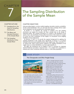
7
Sample Variability
7.1 Sampling Distributions
A distribution of repeated values for
a sample statistic
7.2 The Sampling Distribution
of Sample Means
The theorem describing the distribution
of sample means
7.3 Application of the Sampling
Distribution of Sample Means
The behavior of sample means is predictable.
Image copyright cosma, 2012. Used under license from Shutterstock.com
7.1 Sampling Distributions
Everyday Sampling
Samples are taken every day for many reasons. Industries monitor their products
continually to be sure of their quality, agencies monitor our environment, medical professionals
monitor our health; the list is limitless. Many of these samples are one-time samples, while many
are samples that are repeated for ongoing monitoring.
Population Sampling
A census, a 100% survey or sampling, in the United States is done only every 10 years. It is an
enormous and overwhelming job, but the information that is obtained is vital to our country’s
organization and structure. Issues come up and times change; information is needed and a census
is impractical. This is where representative and everyday samples come in.
313
В© The Jersey Journal/Landov
Sampling Distributions
AP Photo/Toby Talbot
Copyright 2010 Cengage Learning. All Rights Reserved. May not be copied, scanned, or duplicated, in whole or in part. Due to electronic rights, some third party content may be suppressed from the eBook and/or eChapter(s).
Editorial review has deemed that any suppressed content does not materially affect the overall learning experience. Cengage Learning reserves the right to remove additional content at any time if subsequent rights restrictions require it.
Section 7.1
Census enumerator checking data on
a hand-held computer complete with
GPS capabilities to record data
Census worker doing follow-up
Thus to make inferences about a population, we need to discuss sample results a
little more. A sample mean, x, is obtained from a sample. Do you expect this value,
x, to be exactly equal to the value of the population mean, m? Your answer should
be no. We do not expect the means to be identical, but we will be satisfied with our
sample results if the sample mean is “close” to the value of the population mean.
Let’s consider a second question: If a second sample is taken, will the second
sample have a mean equal to the population mean? Equal to the first sample
mean? Again, no, we do not expect the sample mean to be equal to the population
mean, nor do we expect the second sample mean to be a repeat of the first one. We
do, however, again expect the values to be “close.” (This argument should hold for
any other sample statistic and its corresponding population value.)
The next questions should already have come to mind: What is “close”? How do
we determine (and measure) this closeness? Just how will repeated sample statistics
be distributed? To answer these questions we must look at a sampling distribution.
Sampling distribution of a sample statistic The distribution of values for a
sample statistic obtained from repeated samples, all of the same size and
all drawn from the same population.
THE SAMPLING ISSUE
The fundamental goal of a survey
is to come up with the same results
that would have been obtained had
every single member of a population
been interviewed. For national
Gallup polls the objective is to
present the opinions of a sample of
people that are exactly the same
opinions that would have been
obtained had it been possible to
interview all adult Americans in the
country.
The key to reaching this goal is a
fundamental principle called equal
probability of selection, which states
that if every member of a population
has an equal probability of being
selected in a sample, then that
sample will be representative of the
population. It’s that straightforward.
Thus, it is Gallup’s goal in selecting samples to allow every adult
American an equal chance of falling
into the sample. How that is done, of
course, is the key to the success or
failure of the process.
Source: Reprinted by permission of the Gallup Organization, http://www.gallup.com/
314
Chapter 7
Sample Variability
Copyright 2010 Cengage Learning. All Rights Reserved. May not be copied, scanned, or duplicated, in whole or in part. Due to electronic rights, some third party content may be suppressed from the eBook and/or eChapter(s).
Editorial review has deemed that any suppressed content does not materially affect the overall learning experience. Cengage Learning reserves the right to remove additional content at any time if subsequent rights restrictions require it.
Let’s start by investigating two different small theoretical sampling distributions.
E X A M P L E
7 . 1
FORMING A SAMPLING DISTRIBUTION
OF MEANS AND RANGES
Consider as a population the set of single-digit even integers {0, 2, 4, 6, 8}.
In addition, consider all possible samples of size 2. We will look at two different sampling distributions that might be formed: the sampling distribution of
sample means and the sampling distribution of sample ranges.
First we need to list all possible samples of size 2; there are 25 possible
samples:
TA B L E 7 . 1
Probability Distribution:
Sampling Distribution
of Sample Means
—
x
P( x )
0
1
2
3
4
5
6
7
8
0.04
0.08
0.12
0.16
0.20
0.16
0.12
0.08
0.04
{0,
{0,
{0,
{0,
{0,
—
0
1
2
3
4
P (x)
0.20
0.16
0.12
0.08
0.04
TA B L E 7 . 2
Probability Distribution:
Sampling Distribution
of Sample Ranges
R
P(R )
0
2
4
6
8
0.20
0.32
0.24
0.16
0.08
{2,
{2,
{2,
{2,
{2,
0}
2}
4}
6}
8}
{4,
{4,
{4,
{4,
{4,
0}
2}
4}
6}
8}
{6,
{6,
{6,
{6,
{6,
0}
2}
4}
6}
8}
{8,
{8,
{8,
{8,
{8,
0}
2}
4}
6}
8}
FYI Samples
are drawn with
replacement.
x . These means are, respectively:
Each of these samples has a mean —
FIGURE 7.1
Histogram: Sampling
Distribution of Sample Means
0 1 2 3 4 5 6 7 8
0}
2}
4}
6}
8}
x
1
2
3
4
5
2
3
4
5
6
3
4
5
6
7
4
5
6
7
8
Each of these samples is equally likely, and thus each of the 25 sample
1
П­ 0.04. The sampling distribumeans can be assigned a probability of 25
tion of sample means is shown in Table 7.1 as a probability distribution and
shown in Figure 7.1 as a histogram.
For the same set of all possible samples of size 2, let’s find the sampling
distribution of sample ranges. Each sample has a range R. The ranges are:
0
2
4
6
8
2
0
2
4
6
4
2
0
2
4
6
4
2
0
2
8
6
4
2
0
Again, each of these 25 sample ranges has a probability of 0.04. Table 7.2
shows the sampling distribution of sample ranges as a probability distribution,
and Figure 7.2 shows the sampling distribution as a histogram.
FIGURE 7.2
Histogram: Sampling Distribution
of Sample Ranges
P (R)
0.32
0.24
0.16
0.08
0
2
4
6
8
R
Example 7.1 is theoretical in nature and therefore expressed in probabilities. Since
this population is small, it is easy to list all 25 possible samples of size 2 (a sample
space) and assign probabilities. However, it is not always possible to do this.
Section 7.1
Sampling Distributions
315
E X A M P L E
7 . 2
CREATING A SAMPLING DISTRIBUTION OF SAMPLE MEANS
Let’s consider a population that consists of five equally likely integers: 1, 2,
3, 4, and 5. Figure 7.3 shows a histogram representation of the population.
We can observe a portion of the sampling distribution of sample means
when 30 samples of size 5 are randomly selected.
Table 7.3 shows 30 samples and their means. The resulting sampling distribution, a frequency distribution, of sample means is shown in Figure 7.4.
Notice that this distribution of sample means does not look like the population. Rather, it seems to display the characteristics of a normal distribution:
it is mounded and nearly symmetrical about its mean (approximately 3.0).
TA B L E 7 . 3
30 Samples of Size 5 [TA07-03]
FIGURE 7.3
The Population: Theoretical Probability
Distribution
No. Sample
P(x) = 0.2, for x = 1, 2, 3, 4, 5
P(x)
0.20
draw
samples
0.10
вђ® = 3.0
вђґ = 1.41
0.00
1
2
3
x
4
x
x
No. Sample
1
2
3
4
5
4,5,1,4,5
1,1,3,5,1
2,5,1,5,1
4,3,3,1,1
1,2,5,2,4
3.8
2.2
2.8
2.4
2.8
16
17
18
19
20
4,5,5,3,5
3,3,1,2,1
2,1,3,2,2
4,3,4,2,1
5,3,1,4,2
4.4
2.0
2.0
2.8
3.0
6
7
8
9
10
4,2,2,5,4
1,4,5,5,2
4,5,3,1,2
5,3,3,3,5
5,2,1,1,2
3.4
3.4
3.0
3.8
2.2
21
22
23
24
25
4,4,2,2,5
3,3,5,3,5
3,4,4,2,2
3,3,4,5,3
5,1,5,2,3
3.4
3.8
3.0
3.6
3.2
11
12
13
14
15
2,1,4,1,3
5,4,3,1,1
1,3,1,5,5
3,4,5,1,1
3,1,5,3,1
2.2
2.8
3.0
2.8
2.6
26
27
28
29
30
3,3,3,5,2
3,4,4,4,4
2,3,2,4,1
2,1,1,2,4
5,3,3,2,5
3.2
3.8
2.4
2.0
3.6
5
using
the
30
means
Samples of Size 5
FIGURE 7.4
Empirical Distribution of Sample
Means
6
5
Frequency
Copyright 2010 Cengage Learning. All Rights Reserved. May not be copied, scanned, or duplicated, in whole or in part. Due to electronic rights, some third party content may be suppressed from the eBook and/or eChapter(s).
Editorial review has deemed that any suppressed content does not materially affect the overall learning experience. Cengage Learning reserves the right to remove additional content at any time if subsequent rights restrictions require it.
Now, let’s empirically (that is, by experimentation) investigate another sampling distribution.
4
—
x = 2.98
sx = 0.638
3
2
1
0
1.8
2.2
2.6
3.0
3.4
3.8
Sample mean
Video tutorial available—logon and learn more at cengagebrain.com
4.2
4.6
316
Chapter 7
Sample Variability
Copyright 2010 Cengage Learning. All Rights Reserved. May not be copied, scanned, or duplicated, in whole or in part. Due to electronic rights, some third party content may be suppressed from the eBook and/or eChapter(s).
Editorial review has deemed that any suppressed content does not materially affect the overall learning experience. Cengage Learning reserves the right to remove additional content at any time if subsequent rights restrictions require it.
Note: The variable for the sampling distribution is x; therefore, the mean of the x’s
—
is x and the standard deviation of x is sx.
The theory involved with sampling distributions that will be described in the
remainder of this chapter requires random sampling.
Random sample A sample obtained in such a way that each possible sample
of fixed size n has an equal probability of being selected (see p.20).
Figure 7.5 shows how the sampling distribution of sample means is formed.
F I G U R E 7 . 5 The Sampling Distribution of Sample Means
Statistical
population
being
studied
Repeated
sampling is
needed to
form
the sampling
distribution.
All possible
samples
of size n
Sample
1
...
Statistical
Population
The Sampling
Distribution
of Sample Means
x1
x2
xn
The elements of the sampling distribution:
x1
x3
Sample
2
...
Then all of these
values of the sample
statistic, x, are used
to form the sampling
distribution.
x3
x1
Parameter
of interest,
вђ®
One value of the sample
statistic (x in this case)
corresponding to the
parameter of interest
( in this case) is
obtained from each
sample
{x1, x2, x3, ...}
x2
x2
xn
Graphic description of sampling distribution:
Sampling Distribution of Sample Means
P(x)
x3
x2
xn
Sample
3
0.20
x1
x3
0.10
...
0.00
...
x
Sample means
Numerical description of sampling distribution:
All other samples
x1 x2 x3 . . . xn
...
A P P L I E D
E X A M P L E
Many more
x values
вђ®x = вђ® and вђґx =
вђґ
в€љn
7 . 3
AVERAGE AGE OF URBAN TRANSIT RAIL VEHICLES
There are many reasons for collecting data repeatedly. Not all repeated data
collections are performed in order to form a sampling distribution. Consider
the “Average Age of Urban Transit Rail Vehicles (Years)” statistics from the
U.S. Department of Transportation that follow. The table shows the average
age for four different classifications of transit rail vehicles tracked over several years. By studying the pattern of change in the average age for each
class of vehicle, a person can draw conclusions about what has been happening to the fleet over several years. Chances are the people involved in
maintaining each fleet can also detect when a change in policies regarding
Copyright 2010 Cengage Learning. All Rights Reserved. May not be copied, scanned, or duplicated, in whole or in part. Due to electronic rights, some third party content may be suppressed from the eBook and/or eChapter(s).
Sampling Distributions
317
replacement of older vehicles is needed. However useful this information is,
there is no sampling distribution involved here.
Average Age of Urban Transit Rail Vehicles (Years)
1985
1990
Transit rail
Commuter rail locomotivesa
16.3
15.7
Commuter rail passenger coaches
19.1
17.6
Heavy-rail passenger cars
17.1
16.2
Light-rail vehicles (streetcars)
20.6
15.2
1995
2000
2003
2007
15.9
21.4
19.3
16.8
13.4
16.9
22.9
16.1
16.6
20.5
19.0
15.6
18.4
18.9
21.6
16.1
a
Locomotives used in Amtrak intercity passenger services are not included.
Source: U.S. Department of Transportation, Federal Transit Administration
S E C T I O N
7 . 1
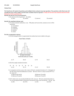
7.1 [EX07-01] Suppose a random sample of 100 ages
was taken from the 2000 census distribution.
45
87
59
39
52
47
35
58
80
2
78
78
8
74
84
11
24
44
41
10
55
7
15
34
27
17
30
30
30
21
15
7
20
6
53
3
37
45
57
19
47
94
49
46
33
31
54
15
63
5
85
48
66
8
48
43
90
25
79
62
93
11
11
46
80
46
26
47
75
32
46
41
61
21
6
23
55
13
7
59
13
81
16
44
62
52
89
28
26
40
41
32
19
41
21
20
2
10
4
16
E X E R C I S E S
These samples could be people, manufactured parts,
or even samples during the manufacturing of potato
chips.
a.
Do you think that all random samples taken from
the same population will lead to the same result?
b.
What characteristic (or property) of random samples could be observed during the sampling
process?
a.
How would you describe the “ages” sample data
above graphically? Construct the graph.
7.4 Refer to Table 7.1 in Example 7.1 (p. 314) and
explain why the samples are equally likely; that is, why
P(0) П­ 0.04, and why P(2) П­ 0.12.
b.
Using the graph that you constructed in part a,
describe the shape of the distribution of the
sample data.
7.5 a.
c.
If another sample were to be collected, would you
expect the same results? Explain.
7.2 a.
What numerical statistics would you use to
describe the “ages” sample data in Exercise 7.1?
Calculate those statistics.
According to the 2000 census (2010 census is not
complete), 275 million Americans have a mean
age of 36.5 years and a standard deviation of
22.5 years.
b.
c.
How well do the statistics calculated in part a
compare to the parameters from the 2000 census?
Be specific.
If another sample were to be collected, would
you expect the same results? Explain.
7.3 Manufacturers use random samples to test
whether or not their product is meeting specifications.
b.
What is a sampling distribution of sample
means?
A sample of size 3 is taken from a population,
and the sample mean is found. Describe how
this sample mean is related to the sampling distribution of sample means.
7.6 Consider the set of odd single-digit integers
{1, 3, 5, 7, 9}.
a.
Make a list of all samples of size 2 that can be
drawn from this set of integers. (Sample with
replacement; that is, the first number is drawn,
observed, and then replaced [returned to the sample
set] before the next drawing.)
b.
Construct the sampling distribution of sample
means for samples of size 2 selected from this set.
c.
Construct the sampling distributions of sample
ranges for samples of size 2.
7.7 Consider the set of even single-digit integers {0, 2,
4, 6, 8}.
[EX00-000] identifies the filename of an exercise’s online dataset—available through cengagebrain.com
Editorial review has deemed that any suppressed content does not materially affect the overall learning experience. Cengage Learning reserves the right to remove additional content at any time if subsequent rights restrictions require it.
Section 7.1
318
Copyright 2010 Cengage Learning. All Rights Reserved. May not be copied, scanned, or duplicated, in whole or in part. Due to electronic rights, some third party content may be suppressed from the eBook and/or eChapter(s).
Editorial review has deemed that any suppressed content does not materially affect the overall learning experience. Cengage Learning reserves the right to remove additional content at any time if subsequent rights restrictions require it.
a.
Chapter 7
Sample Variability
Make a list of all the possible samples of size 3 that
can be drawn from this set of integers. (Sample with
replacement; that is, the first number is drawn,
observed, and then replaced [returned to the sample
set] before the next drawing.)
b.
Construct the sampling distribution of the sample
medians for samples of size 3.
c.
Construct the sampling distribution of the sample
means for samples of size 3.
7.8 Using the phone numbers listed in your telephone
directory as your population, randomly obtain 20 samples
of size 3. From each phone number identified as a source,
take the fourth, fifth, and sixth digits. (For example, for
245-8268, you would take the 8, the 2, and the 6 as your
sample of size 3.)
a.
Calculate the mean of the 20 samples.
b.
Draw a histogram showing the 20 sample means. (Use
classes ПЄ0.5 to 0.5, 0.5 to 1.5, 1.5 to 2.5, and so on.)
c.
Describe the distribution of x’s that you see in
part b (shape of distribution, center, and amount
of dispersion).
d. Draw 20 more samples and add the 20 new x’s to
the histogram in part b. Describe the distribution
that seems to be developing.
7.9 Using a set of five dice, roll the dice and determine
the mean number of dots showing on the five dice.
Repeat the experiment until you have 25 sample
means.
a.
Draw a dotplot showing the distribution of the 25
sample means. (See Example 7.2, p. 315.)
b.
Describe the distribution of x’s in part a.
c.
Repeat the experiment to obtain 25 more sample
means and add these 25 x’s to your dotplot.
Describe the distribution of 50 means.
7.10 Considering the population of five equally likely
integers in Example 7.2:
a.
Verify m and s for the population in Example 7.2.
b.
Table 7.3 lists 30 x values. Construct a grouped frequency distribution to verify the frequency distribution shown in Figure 7.4.
c.
Find the mean and standard deviation of the
—
30 x values in Table 7.3 to verify the values for x
and sx. Explain the meaning of the two symbols
—
x and sx.
7.11 In reference to Applied Example 7.3 on page 316:
a.
Explain why the numerical values on this table do
not form a sampling distribution.
b.
Explain how this repeated gathering of data differs
from the idea of repeated sampling to gather information about a sampling distribution.
7.12 From the table of random numbers in Table 1 in
Appendix B, construct another table showing 20 sets of 5
randomly selected single-digit integers. Find the mean of
each set (the grand mean) and compare this value with
the theoretical population mean, m, using the absolute
difference and the % error. Show all work.
7.13 a.
Using a computer or a random number table,
simulate the drawing of 100 samples, each of
size 5, from the uniform probability distribution
of single-digit integers, 0 to 9.
b.
Find the mean for each sample.
c.
Construct a histogram of the sample means.
(Use integer values as class midpoints.)
d. Describe the sampling distribution shown in
the histogram in part c.
MINITAB
a. Use the Integer RANDOM DATA commands on page 91,
replacing generate with 100, store in with C1–C5,
minimum value with 0, and maximum value with 9.
b. Choose:
Calc>Row Statistics
Select:
Mean
Enter:
Input variables: C1–C5
Store result in: C6>OK
c. Use the HISTOGRAM commands on page 53 for the data
in C6. To adjust the histogram, select Binning with midpoint and midpoint positions 0:9/1.
Excel
a. Input 0 through 9 into column A and corresponding 0.1’s
into column B; then continue with:
Choose:
Enter:
Select:
Enter:
Data>Data Analysis>
Random Number Generation>OK
Number of Variables: 5
Number of Random Numbers: 100
Distribution: Discrete
Value and Probability Input Range:
(A1:B10 or select cells)
Output Range:
(C1 or select cell)>OK
b. Activate cell H1.
Choose:
Enter:
Drag:
Insert function, fx>Statistical>
AVERAGE>OK
Number1: (C1:G1 or select cells)
Bottom right corner of average value box
down to give other averages
c. Use the HISTOGRAM commands on pages 53–54 with column H as the input range and column A as the bin range.
Copyright 2010 Cengage Learning. All Rights Reserved. May not be copied, scanned, or duplicated, in whole or in part. Due to electronic rights, some third party content may be suppressed from the eBook and/or eChapter(s).
Editorial review has deemed that any suppressed content does not materially affect the overall learning experience. Cengage Learning reserves the right to remove additional content at any time if subsequent rights restrictions require it.
Section 7.2
The Sampling Distribution of Sample Means
319
TI-83/84 Plus
MINITAB
a. Use the Integer RANDOM DATA and STO commands on
page 91, replacing the Enter with 0,9,100). Repeat preceding commands four more times, storing data in L2, L3,
L4, and L5, respectively.
b. Choose:
STAT>EDIT>1: Edit
Highlight: L6 (column heading)
Enter:
( L1 Ш‰ L2 Ш‰ L3 Ш‰ L4 Ш‰ L5)/5
c. Choose:
2nd>STAT PLOT>1: Plot1
Choose:
Window
Enter:
0, 9, 1, 0, 30, 5, 1
Choose:
Trace>
>
>
a. Use the Normal RANDOM DATA commands on page 91,
replacing generate with 200, store in with C1–C10, mean
with 100, and standard deviation with 20.
b. Choose:
Calc>Row Statistics
Select:
Mean
Enter:
Input variables: C1–C10
Store result in: C11>OK
c. Use the HISTOGRAM commands on page 53 for the data
in C11. To adjust the histogram, select Binning with midpoint and midpoint positions 74.8:125.2/6.3.
Excel
a. Use the Normal RANDOM NUMBER GENERATION commands on page 91, replacing number of variables with
10, number of random numbers with 200, mean with
100, and standard deviation with 20.
b. Activate cell K1.
Choose:
Enter:
Drag:
7.14 a.
Using a computer or a random number table,
simulate the drawing of 250 samples, each of
size 18, from the uniform probability distribution of single-digit integers, 0 to 9.
b.
Find the mean for each sample.
c.
Construct a histogram of the sample means.
d. Describe the sampling distribution shown in
the histogram in part c.
7.15 a.
Use a computer to draw 200 random samples,
each of size 10, from the normal probability distribution with mean 100 and standard deviation 20.
b.
Find the mean for each sample.
c.
Construct a frequency histogram of the 200
sample means.
d. Describe the sampling distribution shown in
the histogram in part c.
Insert function, f x>Statistical>
AVERAGE>OK
Number1: (A1:J1 or select cells)
Bottom right corner of average value
box down to give other averages
c. Use the RANDOM NUMBER GENERATION Patterned
Distribution commands in Exercise 6.71(a) on page 290,
replacing the first value with 74.8, the last value with
125.2, the steps with 6.3, and the output range with L1.
Use the HISTOGRAM commands on pages 53–54 with
column K as the input range and column L as the bin
range.
7.16 a. Use a computer to draw 500 random samples,
each of size 20, from the normal probability
distribution with mean 80 and standard deviation 15.
b.
Find the mean for each sample.
c.
Construct a frequency histogram of the 500
sample means.
d. Describe the sampling distribution shown in
the histogram in part c, including the mean
and standard deviation.
7.2 The Sampling Distribution
of Sample Means
On the preceding pages we discussed the sampling distributions of two statistics:
sample means and sample ranges. Many others could be discussed; however, the
only sampling distribution of concern to us at this time is the sampling distribution of sample means.
320
FYI This is very
Copyright 2010 Cengage Learning. All Rights Reserved. May not be copied, scanned, or duplicated, in whole or in part. Due to electronic rights, some third party content may be suppressed from the eBook and/or eChapter(s).
Editorial review has deemed that any suppressed content does not materially affect the overall learning experience. Cengage Learning reserves the right to remove additional content at any time if subsequent rights restrictions require it.
useful information!
Chapter 7
Sample Variability
Sampling distribution of sample means (SDSM) If all possible random samples, each of size n, are taken from any population with mean m and standard deviation s, then the sampling distribution of sample means will have
the following:
1. A mean mx equal to m
2. A standard deviation sx equal to
s
в€љ
n
Furthermore, if the sampled population has a normal distribution, then the
sampling distribution of x— will also be normal for samples of all sizes.
This is a very interesting two-part statement. The first part tells us about the relationship between the population mean and standard deviation, and the sampling
distribution mean and standard deviation for all sampling distributions of sample
means. The standard deviation of the sampling distribution is denoted by sx and
given a specific name to avoid confusion with the population standard deviation, s.
Standard error of the mean (sx ) The standard deviation of the sampling distribution of sample means.
FYI Truly amazing:
—
x is normally distributed when n is large
enough, no matter
what shape the
population is!
The second part indicates that this information is not always useful. Stated differently, it says that the mean value of only a few observations will be normally distributed when samples are drawn from a normally distributed population, but it will
not be normally distributed when the sampled population is uniform, skewed, or
otherwise not normal. However, the central limit theorem gives us some additional
and very important information about the sampling distribution of sample means.
Central limit theorem (CLT) The sampling distribution of sample means will
more closely resemble the normal distribution as the sample size increases.
If the sampled distribution is normal, then the sampling distribution of sample means (SDSM) is normal, as stated previously, and the central limit theorem
(CLT) is not needed. But, if the sampled population is not normal, the CLT tells
us that the sampling distribution will still be approximately normally distributed
under the right conditions. If the sampled population distribution is nearly normal, the x distribution is approximately normal for fairly small n (possibly as
small as 15). When the sampled population distribution lacks symmetry, n may
have to be quite large (maybe 50 or more) before the normal distribution
provides a satisfactory approximation.
By combining the preceding information, we can describe the sampling distribution of x completely: (1) the location of the center (mean), (2) a measure of
spread indicating how widely the distribution is dispersed (standard error of the
mean), and (3) an indication of how it is distributed.
1.
2.
3.
mx П­ m; the mean of the sampling distribution (mx) is equal to the mean
of the population (m).
sx П­ в€љsn ; the standard error of the mean (sx) is equal to the standard
deviation of the population (s) divided by the square root of the sample
size, n.
The distribution of sample means is normal when the parent population
is normally distributed, and the CLT tells us that the distribution of sample means becomes approximately normal (regardless of the shape of the
parent population) when the sample size is large enough.
Copyright 2010 Cengage Learning. All Rights Reserved. May not be copied, scanned, or duplicated, in whole or in part. Due to electronic rights, some third party content may be suppressed from the eBook and/or eChapter(s).
Editorial review has deemed that any suppressed content does not materially affect the overall learning experience. Cengage Learning reserves the right to remove additional content at any time if subsequent rights restrictions require it.
Section 7.2
The Sampling Distribution of Sample Means
321
Note: The n referred to is the size of each sample in the sampling distribution.
(The number of repeated samples used in an empirical situation has no effect on
the standard error.)
We do not show the proof for the preceding three facts in this text; however,
their validity will be demonstrated by examining two examples. For the first
example, let’s consider a population for which we can construct the theoretical
sampling distribution of all possible samples.
E X A M P L E
7 . 4
CONSTRUCTING A SAMPLING DISTRIBUTION OF SAMPLE
MEANS
Let’s consider all possible samples of size 2 that could be drawn from a population that contains the three numbers 2, 4, and 6. First let’s look at the population itself. Construct a histogram to picture its distribution, Figure 7.6;
calculate the mean, m, and the standard deviation, s, Table 7.4.
(Remember: We must use the techniques from Chapter 5 for discrete probability distributions.)
FIGURE 7.6
Population
TA B L E 7 . 4
Extensions Table for x
P(x) = 1, for x = 2, 4, 6
x
3
P(x)
2
0.30
4
0.20
6
0.10
вЊє
P(x)
xP(x)
x2P(x)
1
3
1
3
1
3
2
3
4
3
6
3
4
3
16
3
36
3
12
3
56
3
4.0
18.66
3
ck
3
1.0
m П­ 4.0
0.00
2
3
4
x
5
6
s П­ 318.66 ПЄ (4.0)2 П­ 22.66 П­ 1.63
Table 7.5 lists all the possible samples of size 2 that can be drawn from
this population. (One number is drawn, observed, and then returned to the
population before the second number is drawn.) Table 7.5 also lists the means
of these samples. The sample means are then collected to form the sampling
distribution. The distribution for these means and the extensions are given in
Table 7.6 (p. 322, along with the calculation of the mean and the standard
error of the mean for the sampling distribution. The histogram for the sampling
distribution of sample means is shown in Figure 7.7 (p. 322).
TA B L E 7 . 5
All Nine Possible Samples of Size 2
Sample
—
x
Sample
—
x
Sample
—
x
2,2
2,4
2,6
2
3
4
4,2
4,4
4,6
3
4
5
6,2
6,4
6,6
4
5
6
Video tutorial available—logon and learn more at cengagebrain.com
Copyright 2010 Cengage Learning. All Rights Reserved. May not be copied, scanned, or duplicated, in whole or in part. Due to electronic rights, some third party content may be suppressed from the eBook and/or eChapter(s).
Editorial review has deemed that any suppressed content does not materially affect the overall learning experience. Cengage Learning reserves the right to remove additional content at any time if subsequent rights restrictions require it.
322
Chapter 7
Sample Variability
FIGURE 7.7
Sampling Distribution of Sample
Means
TA B L E 7 . 6
x
Extensions Table for —
—
x
2
3
4
5
6
—
P(x
)
— —
x
P(x )
—2 —
x
P(x )
1
2
4
9
2
9
6
9
18
9
3
9
12
9
48
9
2
9
10
9
50
9
1
9
6
9
36
9
9
9
36
156
9
вЊє
9
ck
1.0
9
9
4.0
17.33
Samples of size 2
P(x)
0.30
0.20
0.10
0.00
mx П­ 4.0
2
sx П­ 317.33 ПЄ (4.0) П­ 21.33 П­ 1.15
2
3
4
x
5
6
Let’s now check the truth of the three facts about the sampling distribution of sample means:
1. The mean mx of the sampling distribution will equal the mean m of
the population: both m and mx have the value 4.0.
2. The standard error of the mean sx for the sampling distribution will
equal the standard deviation s of the population divided by the
square root of the sample size, n: sx П­ 1.15 and s П­ 1.63, n П­ 2,
s
в€љ
в€љ
П­ 1.63
П­ 1.15; they are equal: sx П­ в€љsn.
n
2
—
—
—
—
—
3. The distribution will become approximately normally distributed: the
histogram in Figure 7.7 very strongly suggests normality.
DID YOU KNOW
Central Limit Theorem
Abraham de Moivre
was a pioneer in the
theory of probability
and published The
Doctrine of Chance,
first in Latin in 1711
and then in expanded
editions in 1718,
1738, and 1756. The
1756 edition contained his most important contribution—the
approximation of the
binomial distributions
for a large number of
(continued)
Example 7.4, a theoretical situation, suggests that all three facts appear to hold
true. Do these three facts hold when actual data are collected? Let’s look back at
Example 7.2 (p. 315) and see if all three facts are supported by the empirical sampling distribution there.
First, let’s look at the population—the theoretical probability distribution
from which the samples in Example 7.2 were taken. Figure 7.3 is a histogram
showing the probability distribution for randomly selected data from the
population of equally likely integers 1, 2, 3, 4, 5. The population mean m equals
3.0. The population standard deviation s is 12, or 1.41. The population has a
uniform distribution.
Now let’s look at the empirical distribution of the 30 sample means found in
Example 7.2. From the 30 values of x in Table 7.3, the observed mean of the x’s, x,
is 2.98 and the observed standard error of the mean, sx, is 0.638. The histogram of
the sampling distribution in Figure 7.4 appears to be mounded, approximately
symmetrical, and centered near the value 3.0.
Now let’s check the truth of the three specific properties:
1.
mx and m will be equal. The mean of the population m is 3.0, and the
—
observed sampling distribution mean x is 2.98; they are very close in value.
Section 7.2
Copyright 2010 Cengage Learning. All Rights Reserved. May not be copied, scanned, or duplicated, in whole or in part. Due to electronic rights, some third party content may be suppressed from the eBook and/or eChapter(s).
Editorial review has deemed that any suppressed content does not materially affect the overall learning experience. Cengage Learning reserves the right to remove additional content at any time if subsequent rights restrictions require it.
2.
(Continued)
trials using the normal
distribution. The definition of statistical independence also made
its debut along with
many dice and other
games. de Moivre
proved that the central
limit theorem holds for
numbers resulting from
games of chance.
With the use of mathematics, he also successfully predicted the
date of his own death.
3.
The Sampling Distribution of Sample Means
323
в€љ П­ 0.632, and
sx will equal в€љsn. s П­ 1.41 and n П­ 5; therefore, в€љsn П­ 1.41
5
sx П­ 0.638; they are very close in value. (Remember that we have taken
only 30 samples, not all possible samples, of size 5.)
The sampling distribution of x will be approximately normally distributed. Even though the population has a rectangular distribution, the histogram in Figure 7.4 suggests that the x distribution has some of the
properties of normality (mounded, symmetrical).
Although Examples 7.2 and 7.4 do not constitute a proof, the evidence seems
to strongly suggest that both statements, the sampling distribution of sample
means and the CLT, are true.
Having taken a look at these two specific examples, let’s now look at four
graphic illustrations that present the sampling distribution information and the
CLT in a slightly different form. Each of these illustrations has four distributions.
The first graph shows the distribution of the parent population, the distribution
of the individual x values. Each of the other three graphs shows a sampling distribution of sample means, x’s, using three different sample sizes.
In Figure 7.8 we have a uniform distribution, much like Figure 7.3 for the integer illustration, and the resulting distributions of sample means for samples of
sizes 2, 5, and 30.
(d) Sampling
distribution of x
when n = 30
FIGURE 7.8
Uniform Distribution
(a) Population
Values of x
(b) Sampling
distribution of x
when n = 2
Values of x
(c) Sampling
distribution of x
when n = 5
Values of x
Values of x
Figure 7.9 shows a U-shaped population and the three sampling distributions.
(d) Sampling
distribution of x
when n = 30
FIGURE 7.9
U-Shaped Distribution
(a) Population
(b) Sampling
distribution of x
when n = 2
(c) Sampling
distribution of x
when n = 5
Values of x
Values of x
Values of x
Values of x
324
Chapter 7
Sample Variability
Copyright 2010 Cengage Learning. All Rights Reserved. May not be copied, scanned, or duplicated, in whole or in part. Due to electronic rights, some third party content may be suppressed from the eBook and/or eChapter(s).
Editorial review has deemed that any suppressed content does not materially affect the overall learning experience. Cengage Learning reserves the right to remove additional content at any time if subsequent rights restrictions require it.
Figure 7.10 shows a J-shaped population and the three sampling
distributions.
(d) Sampling
distribution of x
when n = 30
FIGURE 7.10
J-Shaped Distribution
(a) Population
(b) Sampling
distribution of x
when n = 2
(c) Sampling
distribution of x
when n = 5
Values of x
Values of x
Values of x
Values of x
All three nonnormal population distributions seem to verify the CLT; the
sampling distributions of sample means appear to be approximately normal for
all three when samples of size 30 are used. Now consider Figure 7.11, which
shows a normally distributed population and the three sampling distributions.
With the normal population, the sampling distributions of the sample means for
all sample sizes appear to be normal. Thus, you have seen an amazing phenomenon: No matter what the shape of a population, the sampling distribution of
sample means either is normal or becomes approximately normal when n
becomes sufficiently large.
(d) Sampling
distribution of x
when n = 30
FIGURE 7.11
Normal Distribution
(a) Population
(b) Sampling
distribution of x
when n = 2
(c) Sampling
distribution of x
when n = 5
Values of x
Values of x
Values of x
Values of x
You should notice one other point: The sample mean becomes less variable as
the sample size increases. Notice that as n increases from 2 to 30, all the distributions become narrower and taller.
Section 7.2
Copyright 2010 Cengage Learning. All Rights Reserved. May not be copied, scanned, or duplicated, in whole or in part. Due to electronic rights, some third party content may be suppressed from the eBook and/or eChapter(s).
7 . 2
7.17 Skillbuilder Applet
Exercise simulates taking
samples of size 4 from an
approximately normal population, where m П­ 65.15 and
s П­ 2.754.
a.
Click “1” for “# Samples.”
Note the four data values and their mean. Change
“slow” to “batch” and take at least 1000 samples
using the “500” for “# Samples.”
325
E X E R C I S E S
7.20 If a population has a standard deviation s of
25 units, what is the standard error of the mean if samples
of size 16 are selected? Samples of size 36? Samples of
size 100?
7.21 A certain population has a mean of 500 and a standard deviation of 30. Many samples of size 36 are randomly selected and the means calculated.
a.
What value would you expect to find for the mean
of all these sample means?
b.
What is the mean for the 1001 sample means? How
close is it to the population mean, m?
b.
What value would you expect to find for the standard deviation of all these sample means?
c.
Compare the sample standard deviation to the population standard deviation, s. What is happening to
the sample standard deviation? Compare it with
s/1n, which is 2.754/14.
c.
What shape would you expect the distribution of all
these sample means to have?
d. Does the histogram of sample means have an
approximately normal shape?
e.
Relate your findings to the SDSM.
7.18 Skillbuilder Applet Exercise simulates sampling from a
skewed population, where
m П­ 6.029 and s П­ 10.79.
a.
b.
c.
Change the “#
Observations per sample” to “4.” Using batch
and 500, take 1000
samples of size 4.
Compare the mean and standard deviation for the
sample means with m and s. Compare the sample
standard deviation with s/1n, which is 10.79/14.
Does the histogram have an approximately normal
shape? If not, what shape is it?
Using the “clear” button each time, repeat the
directions in parts a and b for samples of size 25,
100, and 1000. Table your findings for each
sample size.
d. Relate your findings to the SDSM and the CLT.
7.19 a.
b.
What is the total measure of the area for any
probability distribution?
Justify the statement “x becomes less variable
as n increases.”
7.22 According to Nielsen’s Television Audience Report,
in 2009 the average American home had 2.86 television
sets (more than the average number of people per
household, at 2.5 people). If the standard deviation for
the number of televisions in a U.S. household is 1.2 and
a random sample of 80 American households is
selected, the mean of this sample belongs to a sampling
distribution.
a.
What is the shape of this sampling distribution?
b.
What is the mean of this sampling distribution?
c.
What is the standard deviation of this sampling
distribution?
7.23 The September 21, 2006, USA Today article
“Average home has more TVs than people” stated that
Americans watch an average of 4.58 hours of television
per person per day.
Source: Nielsen Media Research
If the standard deviation for the number of hours of
television watched per day is 2.1 and a random sample of
250 Americans is selected, the mean of this sample
belongs to a sampling distribution.
a.
What is the shape of this sampling distribution?
b.
What is the mean of this sampling distribution?
c.
What is the standard deviation of this sampling
distribution?
7.24 According to The World Factbook, 2009, the total
fertility rate (estimated mean number of children born
per woman) for Uganda is 6.77. Suppose that the standard deviation of the total fertility rate is 2.6. The mean
number of children for a sample of 200 randomly
(continue on page 326)
Skillbuilder Applets are available online through cengagebrain.com.
Editorial review has deemed that any suppressed content does not materially affect the overall learning experience. Cengage Learning reserves the right to remove additional content at any time if subsequent rights restrictions require it.
S E C T I O N
The Sampling Distribution of Sample Means
326
Chapter 7
Sample Variability
Copyright 2010 Cengage Learning. All Rights Reserved. May not be copied, scanned, or duplicated, in whole or in part. Due to electronic rights, some third party content may be suppressed from the eBook and/or eChapter(s).
Editorial review has deemed that any suppressed content does not materially affect the overall learning experience. Cengage Learning reserves the right to remove additional content at any time if subsequent rights restrictions require it.
selected women is one value of many that form the sampling distribution of sample means.
a.
What is the mean value for this sampling
distribution?
b.
What is the standard deviation of this sampling
distribution?
c.
Describe the shape of this sampling distribution.
7.25 The American Meat Institute published the 2007
report “U.S. Meat and Poultry Production & Consumption:
An Overview.” The 2007 Fact Sheet lists the annual
consumption of chicken as 86.5 pounds per person.
Suppose the standard deviation for the consumption of
chicken per person is 29.3 pounds. The mean weight of
chicken consumed for a sample of 150 randomly selected
people is one value of many that form the sampling distribution of sample means.
a.
What is the mean value for this sampling
distribution?
b.
What is the standard deviation of this sampling
distribution?
c.
Describe the shape of this sampling distribution.
7.26 A researcher wants to take a simple random sample
of about 5% of the student body at each of two schools.
The university has approximately 20,000 students, and
the college has about 5000 students. Identify each of the
following as true or false and justify your answer.
a.
The sampling variability is the same for both schools.
b.
The sampling variability for the university is higher
than that for the college.
c.
The sampling variability for the university is lower
than that for the college.
d. No conclusion about the sampling variability can be
stated without knowing the results of the study.
7.27 a.
Use a computer to randomly select 100 samples
of size 6 from a normal population with mean
m П­ 20 and standard deviation s П­ 4.5.
b.
Find mean x for each of the 100 samples.
c.
Using the 100 sample means, construct a his—
togram, find mean x, and find the standard
deviation sx.
MINITAB
a. Use the Normal RANDOM DATA commands on page 91,
replacing generate with 100, store in with C1–C6, mean
with 20, and standard deviation with 4.5.
b. Use the ROW STATISTICS commands on page 318,
replacing input variables with C1–C6 and store result in
with C7.
c. Use the HISTOGRAM commands on page 53 for the data
in C7. To adjust the histogram, select Binning with midpoint and midpoint positions 12.8:27.2/1.8. Use the
MEAN and STANDARD DEVIATION commands on
pages 65 and 79 for the data in C7.
Excel
a. Use the Normal RANDOM NUMBER GENERATION commands on page 91, replacing number of variables with 6,
number of random numbers with 100, mean with 20, and
standard deviation with 4.5.
b. Activate cell G1.
Choose:
Insert function, fx>Statistical>
AVERAGE>OK
Number1: (A1:F1 or select cells)
Bottom right corner of average value
box down to give other averages
Enter:
Drag:
c. Use the RANDOM NUMBER GENERATION Patterned
Distribution commands in Exercise 6.71(a) on page 291
replacing the first value with 12.8, the last value with
27.2, the steps with 1.8, and the output range with
H1. Use the HISTOGRAM commands on pages 53–54
with column G as the input range and column H as
the bin range. Use the MEAN and STANDARD
DEVIATION commands on pages 65 and 79 for the data
in column G.
TI-83/84 Plus
a. Use the Normal RANDOM DATA and STO commands on
page 91, replacing Enter with 20, 4.5,100). Repeat the
preceding commands five more times, storing data in L2,
L3, L4, L5, and L6, respectively.
b. Enter:
Choose:
(L1 Ш‰ L2 Ш‰ L3 Ш‰ L4 Ш‰ L5 Ш‰ L6)/6
STO S L7 (use ALPHA key for the “L” or
use “MEAN”)
c. Choose:
Choose:
Enter:
Choose:
Choose:
2 nd>STAT PLOT>1: Plot1
Window
12.8, 27.2, 1.8, 0, 40, 5, 1
Trace>>>
STAT>CALC>
1:1-VAR STATS>2nd>LIST
L7
Select:
Section 7.3
Application of the Sampling Distribution of Sample Means
Copyright 2010 Cengage Learning. All Rights Reserved. May not be copied, scanned, or duplicated, in whole or in part. Due to electronic rights, some third party content may be suppressed from the eBook and/or eChapter(s).
Editorial review has deemed that any suppressed content does not materially affect the overall learning experience. Cengage Learning reserves the right to remove additional content at any time if subsequent rights restrictions require it.
d. Compare the results of part c with the three
statements made in the SDSM.
7.28 a.
Use a computer to randomly select 200 samples
of size 24 from a normal population with mean
m П­ 20 and standard deviation s П­ 4.5.
b.
Find mean x for each of the 200 samples.
c.
Using the 200 sample means, construct a his—
togram, find mean x, and find the standard
deviation sx.
327
d. Compare the results of part c with the three
statements made for the SDSM and CLT on
page 320.
e.
Compare these results with the results
obtained in Exercise 7.27. Specifically, what
effect did the increase in sample size from 6
to 24 have? What effect did the increase from
100 samples to 200 samples have?
FYI If you use a computer, see Exercise 7.27.
7.3 Application of the Sampling
Distribution of Sample Means
When the sampling distribution of sample means is normally distributed, or
approximately normally distributed, we will be able to answer probability questions with the aid of the standard normal distribution (Table 3 of Appendix B).
E X A M P L E
7 . 5
CONVERTING x INFORMATION INTO z-SCORES
Consider a normal population with m П­ 100 and s П­ 20. If a random sample of size 16 is selected, what is the probability that this sample will have
a mean value between 90 and 110? That is, what is P(90 ПЅ x ПЅ 110)?
Solution
x ’s
Since the population is normally distributed, the sampling distribution of —
is normally distributed. To determine probabilities associated with a normal
distribution, we will need to convert the statement P(90 ПЅ x ПЅ 110) to a
probability statement involving the z-score. This will allow us to use Table 3
in Appendix B, the standard normal distribution table. The sampling distribution is shown in the figure, where the shaded area represents
P(90 ПЅ x ПЅ 110).
x is
The formula for finding the z-score corresponding to a known value of —
вђґ x = 20/ 16 = 5
zП­
x ПЄ mx
sx
—
(7.1)
—
The mean and standard error of the mean are mx П­ m and sx П­ в€љsn .
Therefore, we will rewrite formula (7.1) in terms of m, s, and n:
—
90
вђ® = 100
110
zП­
x
—
xПЄm
в€љ
s/ n
Returning to the example and applying formula (7.2), we find:
z-score for x П­ 90:В В В В z П­
x ПЄ m 90 ПЄ 100 ПЄ10
П­
П­
П­ ШЉ2.00
5
s/1n
20/116
(7.2)
Copyright 2010 Cengage Learning. All Rights Reserved. May not be copied, scanned, or duplicated, in whole or in part. Due to electronic rights, some third party content may be suppressed from the eBook and/or eChapter(s).
Editorial review has deemed that any suppressed content does not materially affect the overall learning experience. Cengage Learning reserves the right to remove additional content at any time if subsequent rights restrictions require it.
328
Chapter 7
Sample Variability
z-score for x П­ 110:В В В В z П­
x ПЄ m 110 ПЄ 100 10
П­
П­
П­ 2.00
5
s/1n
20/116
Therefore,
P(90 ПЅ x ПЅ 110) П­ P(ПЄ2.00 ПЅ z ПЅ 2.00) П­ 0.9773 ПЄ 0.0228 П­ 0.9545
Before we look at additional examples, let’s consider what is implied by sx ϭ √sn.
To demonstrate, let’s suppose that s ϭ 20 and let’s use a sampling distribution of
samples of size 4. Now sx is 20/ 14, or 10, and approximately 95% (0.9545) of all such
sample means should be within the interval from 20 below to 20 above the population mean (within 2 standard deviations of the population mean). However, if the
sample size is increased to 16, sx becomes 20/116 П­ 5 and approximately 95% of
the sampling distribution should be within 10 units of the mean, and so on. As the
sample size increases, the size of sx becomes smaller and the distribution of sample
means becomes much narrower. Figure 7.12 illustrates what happens to the distribution of x’s as the size of the individual samples increases.
FIGURE 7.12
Distributions of Sample Means
Distribution of sample means
for larger sample size
Distribution of sample means
for smaller sample size
Recall that the area (probability) under the normal curve is always exactly 1. So
as the width of the curve narrows, the height has to increase to maintain this area.
E X A M P L E
7 . 6
CALCULATING PROBABILITIES FOR THE MEAN HEIGHT
OF KINDERGARTEN CHILDREN
Kindergarten children have heights that are approximately normally distributed about a mean of 39 inches and a standard deviation of 2 inches. A
x is calculated. What is
random sample of size 25 is taken, and the mean —
the probability that this mean value will be between 38.5 and 40.0 inches?
Solution
x , 38.5 and 40.0, must
We want to find P(38.5 Ͻ x Ͻ 40.0). The values of —
be converted to z-scores (necessary for use of Table 3 in Appendix B) using
xПЄm
z П­ s/в€љn :
x П­ 38.5:В В В В z П­
xПЄm
s/1n
П­
38.5 ПЄ 39.0 ПЄ0.5
П­
П­ ШЉ1.25
0.4
2/125
Video tutorial available—logon and learn more at cengagebrain.com
Copyright 2010 Cengage Learning. All Rights Reserved. May not be copied, scanned, or duplicated, in whole or in part. Due to electronic rights, some third party content may be suppressed from the eBook and/or eChapter(s).
Editorial review has deemed that any suppressed content does not materially affect the overall learning experience. Cengage Learning reserves the right to remove additional content at any time if subsequent rights restrictions require it.
Section 7.3
Application of the Sampling Distribution of Sample Means
x П­ 40.0:В В В В z П­
xПЄm
s/1n
П­
329
40.0 ПЄ 39.0 1.0
П­
П­ 2.50
0.4
2/125
Therefore,
P(38.5 ПЅ x ПЅ 40.0) П­ P(ПЄ1.25 ПЅ z ПЅ 2.50) П­ 0.9938 ПЄ 0.1057 П­ 0.8881
38.5 39.0
0
–1.25
E X A M P L E
40.0
2.50
x
z
7 . 7
CALCULATING MEAN HEIGHT LIMITS FOR THE MIDDLE 90%
OF KINDERGARTEN CHILDREN
Use the heights of kindergarten children given in Example 7.6. Within what
limits does the middle 90% of the sampling distribution of sample means for
samples of size 100 fall?
Solution
The two tools we have to work with
are formula (7.2) and Table 3 in
Appendix B. The formula relates the
key values of the population to the
key values of the sampling distribution, and Table 3 relates areas to
z-scores. First, using Table 3, we find
that the middle 0.9000 is bounded
by z П­ П®1.65 .
z
FYI Remember: If
o
ШЉ1.6
o
value is exactly
halfway, use the
larger z.
...
90%
5% or
0.0500
z = –1.65
0.04
...
0.0505
(45%)
(45%)
0.0500
5% or
0.0500
z = 1.65
0
0.05
...
0.0495
...
...
z
—
Second, we use formula (7.2), z П­
x ПЄm
s/ 1n
:
—
z П­ ПЄ1.65:
ПЄ1.65 П­
—
x ПЄ 39.0
2/2100
x ПЄ 39 П­ (ПЄ1.65)(0.2)
—
x П­ 39 ПЄ 0.33
‫ ؍‬38.67
—
z П­ 1.65:
1.65 П­
x ПЄ 39.0
2/ 2100
—
x ПЄ 39 П­ (1.65)(0.2)
—
x П­ 39 П© 0.33
‫ ؍‬39.33
Thus,
— <39.33) ‫ ؍‬0.90
P(38.67<x
Therefore, 38.67 inches and 39.33 inches are the limits that capture the
middle 90% of the sample means.
330
Chapter 7
Copyright 2010 Cengage Learning. All Rights Reserved. May not be copied, scanned, or duplicated, in whole or in part. Due to electronic rights, some third party content may be suppressed from the eBook and/or eChapter(s).
Editorial review has deemed that any suppressed content does not materially affect the overall learning experience. Cengage Learning reserves the right to remove additional content at any time if subsequent rights restrictions require it.
S E C T I O N
Sample Variability
7 . 3
7.29 Consider a normal population with m П­ 43 and
s П­ 5.2. Calculate the z-score for an x of 46.5 from a sample of size 16.
7.30 Consider a population with m П­ 43 and s П­ 5.2.
a.
Calculate the z-score for an x of 46.5 from a sample
of size 35.
b.
Could this z-score be used in calculating probabilities
using Table 3 in Appendix B? Why or why not?
7.31 In Example 7.5, explain how the 0.9773 and the
0.0228 were obtained and what they are used for.
7.32 What is the probability that the sample of kindergarten children in Example 7.6 has a mean height of less
than 39.75 inches?
7.33 A random sample of size 36 is to be selected from a
population that has a mean m П­ 50 and a standard deviation s of 10.
a.
This sample of 36 has a mean value of x, which
belongs to a sampling distribution. Find the shape
of this sampling distribution.
b.
Find the mean of this sampling distribution.
c.
Find the standard error of this sampling distribution.
d. What is the probability that this sample mean will
be between 45 and 55?
e.
What is the probability that the sample mean will
have a value greater than 48?
f.
What is the probability that the sample mean will
be within 3 units of the mean?
7.34 The local bakery bakes more than a thousand 1-pound
loaves of bread daily, and the weights of these loaves vary.
The mean weight is 1 lb and 1 oz, or 482 grams.Assume that
the standard deviation of the weights is 18 grams and that a
sample of 40 loaves is to be randomly selected.
a.
This sample of 40 has a mean value of x, which
belongs to a sampling distribution. Find the shape
of this sampling distribution.
b.
Find the mean of this sampling distribution.
c.
Find the standard error of this sampling distribution.
d. What is the probability that this sample mean will
be between 475 and 495?
e.
What is the probability that the sample mean will
have a value less than 478?
f.
What is the probability that the sample mean will be
within 5 grams of the mean?
E X E R C I S E S
7.35 Consider the approximately normal population of
heights of male college students with mean m П­ 69 inches
and standard deviation s П­ 4 inches. A random sample of
16 heights is obtained.
a.
Describe the distribution of x, height of male college students.
b.
Find the proportion of male college students whose
height is greater than 70 inches.
c.
Describe the distribution of x, the mean of samples
of size 16.
d. Find the mean and standard error of the x distribution.
e.
Find P(x Пѕ 70).
f.
Find P(x ПЅ 67).
7.36 The amount of fill (weight of contents) put into a
glass jar of spaghetti sauce is normally distributed with
mean m П­ 850 grams and standard deviation s П­ 8 grams.
a.
Describe the distribution of x, the amount of fill per
jar.
b.
Find the probability that one jar selected at random
contains between 848 and 855 grams.
c.
Describe the distribution of x, the mean weight for a
sample of 24 such jars of sauce.
d. Find the probability that a random sample of 24 jars
has a mean weight between 848 and 855 grams.
7.37 The heights of the kindergarten children mentioned
in Example 7.6 (p. 328) are approximately normally distributed with m П­ 39 and s П­ 2.
a.
If an individual kindergarten child is selected at random, what is the probability that he or she has a height
between 38 and 40 inches?
b.
A classroom of 30 of these children is used as a
sample. What is the probability that the class mean
x is between 38 and 40 inches?
c.
If an individual kindergarten child is selected at random, what is the probability that he or she is taller
than 40 inches?
d.
A classroom of 30 of these kindergarten children is
used as a sample. What is the probability that the class
mean x is greater than 40 inches?
7.38 Salaries for various positions can vary significantly,
depending on whether or not the company is in the public
or private sector.The U.S. Department of Labor posted the
2007 average salary for human resource managers
employed by the federal government as $76,503. Assume
Section 7.3
Application of the Sampling Distribution of Sample Means
Copyright 2010 Cengage Learning. All Rights Reserved. May not be copied, scanned, or duplicated, in whole or in part. Due to electronic rights, some third party content may be suppressed from the eBook and/or eChapter(s).
Editorial review has deemed that any suppressed content does not materially affect the overall learning experience. Cengage Learning reserves the right to remove additional content at any time if subsequent rights restrictions require it.
that annual salaries for this type of job are normally distributed and have a standard deviation of $8850.
a.
b.
What is the probability that a randomly selected
human resource manager received over $100,000 in
2007?
A sample of 20 human resource managers is taken
and annual salaries are reported. What is the probability that the sample mean annual salary falls
between $70,000 and $80,000?
7.39 Based on data from 1996 through 2006 from the
Western Regional Climate Center, the average speed
of winds in Honolulu, Hawaii, equals 10.6 miles per hour.
Assume that wind speeds are approximately normally distributed with a standard deviation of 3.5 miles per hour.
a.
Find the probability that the wind speed in any one
reading will exceed 13.5 miles per hour.
b.
Find the probability that the mean of a random
sample of 9 readings exceeds 13.5 miles per hour.
c.
Do you think the assumption of normality is reasonable? Explain.
331
b.
Find the probability that the mean cost to attend a
high school prom for 36 randomly selected 17-yearolds is greater than $750.
c.
Do you think the assumption of normality is reasonable? Explain.
7.42 The Bureau of Labor Statistics provides compensation information on and services for various positions. As
of May 2008, the national average salary for an RN (registered nurse) was $65,130. Suppose the standard deviation is $9385. Find the following for the mean of a
random sample of 100 such nurses.
a.
The probability that the mean of the sample is less
than $62,500
b.
The probability that the sample mean is between
$64,000 and $67,500
c.
The probability that the sample mean is greater
than $66,000
d. Explain why the assumption of normality about the
distribution of wages was not involved in the solutions parts to a, b, and c.
d. What effect do you think the assumption of normality had on the answers to parts a and b? Explain.
7.43 Referring to Example 7.6 (p. 328), what height
would bound the lower 25% of all samples of size 25?
7.40 TIMSS 2007 (Trends in International Mathematics
and Science Study) focused on the mathematics and science achievement of eighth-grade students throughout the
world. A total of 8 countries (including the United States)
participated in the study. The mean math exam score for
U.S. students was 509 with a standard deviation of 88.
7.44 A popular flashlight that uses two D-size batteries
was selected, and several of the same models were purchased to test the “continuous-use life” of D batteries. As
fresh batteries were installed, each flashlight was turned
on and the time noted. When the flashlight no longer produced light, the time was again noted. The resulting “life”
data from Rayovac batteries had a mean of 21.0 hours.
Source: http://nces.ed.gov/
Assuming the scores are normally distributed, find the
following for a sample of 150 students.
a.
b.
c.
Find the probability that the mean TIMSS score for
a randomly selected group of eighth-grade students
would be between 495 and 515.
Find the probability that the mean TIMSS score for
a randomly selected group of eighth-grade students
would be less than 520.
Do you think the assumption of normality is reasonable? Explain.
Source: http://www.rayovac.com.
Assume these values have a normal distribution with a
standard deviation of 1.38 hours.
a.
What is the probability that one randomly selected
Rayovac battery will have a test life of between 20.5
and 21.5 hours?
b.
What is the probability that a randomly selected sample of 4 Rayovac batteries will have a mean test life of
between 20.5 and 21.5 hours?
c.
What is the probability that a randomly selected
sample of 16 Rayovac batteries will have a mean
test life of between 20.5 and 21.5 hours?
7.41 According to the June 2004 Readers’ Digest article
“Only in America,” the average amount that a 17-yearold spends on his or her high school prom is $638.
Assume that the amounts spent are normally distributed
with a standard deviation of $175.
d. What is the probability that a randomly selected
sample of 64 Rayovac batteries will have a mean
test life of between 20.5 and 21.5 hours?
a.
e.
Find the probability that the mean cost to attend
a high school prom for 36 randomly selected
17-year-olds is between $550 and $700.
Describe the effect that the increase in sample size
had on the answers for parts b–d.
332
Chapter 7
Copyright 2010 Cengage Learning. All Rights Reserved. May not be copied, scanned, or duplicated, in whole or in part. Due to electronic rights, some third party content may be suppressed from the eBook and/or eChapter(s).
Editorial review has deemed that any suppressed content does not materially affect the overall learning experience. Cengage Learning reserves the right to remove additional content at any time if subsequent rights restrictions require it.
7.45 a.
Sample Variability
Find P(4 ПЅ x ПЅ 6) for a random sample of size 4
drawn from a normal population with m П­ 5
and s П­ 2.
b.
Use a computer to randomly generate 100
samples, each of size 4, from a normal probability distribution with m П­ 5 and s П­ 2.
Calculate the mean, x, for each sample.
c.
How many of the sample means in part b have
values between 4 and 6? What percentage is
that?
d. Compare the answers to parts a and c, and
explain any differences that occurred.
MINITAB
a. Input the numbers 4 and 6 into C1. Use the CUMULATIVE
NORMAL PROBABILITY DISTRIBUTION commands on
page 285, replacing the mean with 5, the standard deviation with 1 (2/24), the input column with C1, and the
optional storage with C2. Find CDF(6) – CDF(4).
b. Use the Normal RANDOM DATA commands on
page 91, replacing generate with 100, store in with
C3–C6, mean with 5, and standard deviation with 2.
Use the ROW STATISTICS commands on page 318,
replacing input variables with C3–C6 and store result
in with C7.
c. Use the HISTOGRAM commands on page 53 for the data
in C7. Select Labels, Data Labels, Label Type; use y-value
levels. To adjust the histogram, select Binning with midpoint and midpoint positions 0:10/1.
commands in Exercise 7.13(b) on page 318, replacing
Number1 with C1:F1.
c. Use the RANDOM NUMBER GENERATION Patterned
Distribution commands in Exercise 6.71(a) on page 291,
replacing the first value with 0, the last value with 9, the
steps with 1, and the output range with H1. Use the HISTOGRAM commands on pages 53–54 with column G as
the input range, column Has the bin range, and column I
as the output range.
TI-83/84 Plus
a. Use the CUMULATIVE NORMAL PROBABILITY commands
on page 285, replacing the Enter with 4,6,5,1). (The standard deviation is 1; from 2/ 24.)
b. Use the Normal RANDOM DATA and STO commands on
page 91, replacing the Enter with 5,2,100). Repeat these
commands three more times, storing data in L2, L3, and
L4, respectively.
Choose:
Highlight:
Enter:
c. Use the HISTOGRAM and TRACE commands on page 54
to count. Enter 0,9,1,0,45,1 for the Window.
7.46 a.
Find P(46 ПЅ x ПЅ 55) for a random sample of
size 16 drawn from a normal population with
mean m П­ 50 and standard deviation s П­ 10.
b.
Use a computer to randomly generate 200
samples, each of size 16, from a normal probability distribution with mean m П­ 50 and standard deviation s П­ 10. Calculate the mean, x,
for each sample.
c.
How many of the sample means in part b have
values between 46 and 55? What percentage is
that?
Excel
a. Input the numbers 4 and 6 into column A. Activate cell
B1. Use the CUMULATIVE NORMAL DISTRIBUTION
commands on page 285, replacing X with A1:A2. Find
CDF(6)–CDF(4).
b. Use the Normal RANDOM NUMBER GENERATION commands on page 91, replacing number of variables with
4, number of random numbers with 100, mean with 5,
standard deviation with 2, and output range with C1.
Activate cell G1. Use the AVERAGE INSERT FUNCTION
STAT> EDIT>1: Edit
L5 (column heading)
(L1 П© L2 П© L3 П© L4)/4
d. Compare the answers to parts a and c, and
explain any differences that occurred.
FYI If you use a computer, see Exercise 7.45.
Image copyright cosma,
2012. Used under
license from
Shutterstock.com
Copyright 2010 Cengage Learning. All Rights Reserved. May not be copied, scanned, or duplicated, in whole or in part. Due to electronic rights, some third party content may be suppressed from the eBook and/or eChapter(s).
Editorial review has deemed that any suppressed content does not materially affect the overall learning experience. Cengage Learning reserves the right to remove additional content at any time if subsequent rights restrictions require it.
Chapter Review
333
Chapter Review
In Retrospect
In Chapters 6 and 7 we have learned to use the standard
normal probability distribution. We now have two formulas for calculating a z-score:
You must be careful to distinguish between these two
formulas. The first gives the standard score when we have
individual values from a normal distribution (x values).
The second formula deals with a sample mean (x value).
The key to distinguishing between the formulas is to
decide whether the problem deals with an individual x or
a sample mean x. If it deals with the individual values of
x, we use the first formula, as presented in Chapter 6. If
the problem deals with a sample mean, x, we use the second formula and proceed as illustrated in this chapter.
The basic purpose for considering what happens when
a population is repeatedly sampled, as discussed in this
chapter, is to form sampling distributions.The sampling distribution is then used to describe the variability that occurs
from one sample to the next. Once this pattern of variability is known and understood for a specific sample statistic,
we are able to make predictions about the corresponding
population parameter with a measure of how accurate the
prediction is. The SDSM and the central limit theorem help
describe the distribution for sample means.We will begin to
make inferences about population means in Chapter 8.
There are other reasons for repeated sampling.
Repeated samples are commonly used in the field of production control, in which samples are taken to determine
whether a product is of the proper size or quantity. When
the sample statistic does not fit the standards, a mechanical adjustment of the machinery is necessary. The adjustment is then followed by another sampling to be sure the
production process is in control.
The “standard error of the _____” is the name used
for the standard deviation of the sampling distribution for
whatever statistic is named in the blank. In this chapter
we have been concerned with the standard error of the
mean. However, we could also work with the standard
error of the proportion, median, or any other statistic.
You should now be familiar with the concept of a
sampling distribution and, in particular, with the sampling distribution of sample means. In Chapter 8 we will
begin to make predictions about the values of population
parameters.
The Statistics CourseMate site
for this text brings chapter topics to life with interactive
learning, study, and exam preparation tools, including
quizzes and flashcards for the Vocabulary and Key
Concepts that follow. The site also provides an eBook
version of the text with highlighting and note taking
capabilities. Throughout chapters, the CourseMate
icon
flags concepts and examples that have
corresponding interactive resources such as video and
animated tutorials that demonstrate, step by step, how to
solve problems; datasets for exercises and examples;
Skillbuilder Applets to help you better understand concepts; technology manuals; and software to download
including Data Analysis Plus (a suite of statistical macros
for Excel) and TI-83/84 Plus programs—logon at
www.cengagebrain.com.
zП­
xПЄm
xПЄm
В andВ z П­
s
s/2n
Vocabulary and Key Concepts
central limit theorem (p. 320)
frequency distribution (p. 315)
probability distribution (p. 314)
random sample (p. 316)
repeated sampling (p. 313)
sampling distribution (p. 323)
sampling distribution of sample
means (pp. 314, 320)
standard error of the mean
(p. 320)
z-score (p. 327)
334
Chapter 7
Sample Variability
Copyright 2010 Cengage Learning. All Rights Reserved. May not be copied, scanned, or duplicated, in whole or in part. Due to electronic rights, some third party content may be suppressed from the eBook and/or eChapter(s).
Editorial review has deemed that any suppressed content does not materially affect the overall learning experience. Cengage Learning reserves the right to remove additional content at any time if subsequent rights restrictions require it.
Learning Outcomes
• Understand what a sampling distribution of a sample statistic is and that
the distribution is obtained from repeated samples, all of the same size.
• Be able to form a sampling distribution for a mean, median, or range based
on a small, finite population.
• Understand that a sampling distribution is a probability distribution for a
sample statistic.
• Understand and be able to present and describe the sampling distribution
of sample means and the central limit theorem.
• Understand and be able to explain the relationship between the
sampling distribution of sample means and the central limit theorem.
• Determine and be able to explain the effect of sample size on the
standard error of the mean.
• Understand when and how the normal distribution can be used to
find probabilities corresponding to sample means.
• Compute, describe, and interpret z-scores corresponding to
known values of x.
• Compute z-scores and probabilities for applications of the sampling
distribution of sample means.
pp. 313–314, EXP 7.1
EXP 7.1, Ex. 7.6, 7.7
EXP 7.2
pp. 319–321, EXP 7.4
pp. 319–321, Ex. 7.17, 7.18, 7.21
pp. 323–324, Ex. 7.20, 7.26, 7.47
EXP 7.5
EXP 7.6, EXP 7.7,
Ex. 7.29, 7.30, 7.48
Ex. 7.33, 7.35
Chapter Exercises
7.47 If a population has a standard deviation s of 18.2
units, what is the standard error of the mean if samples of
size 9 are selected? Samples of size 25? Samples of size
49? Samples of size 100?
If a random sample of 25 graduates is selected:
7.48 Consider a normal population with m П­ 24.7 and
s П­ 4.5.
d. What is the probability that the sample mean is
between $710 and $785?
a. Calculate the z-score for an x of 21.5.
b. Calculate the z-score for an x of 21.5 from a sample
of size 25.
c. Explain how 21.5 can have such different z-scores.
7.49 The dean of nursing tells students being recruited
for the incoming class that the school’s graduates can
expect to earn a mean weekly income of $775 one year
after graduation. Assume that the dean’s statement is
true and that the weekly salaries one year after graduation are normally distributed with a standard deviation
of $115.
If one graduate is randomly selected:
a. Describe the distribution of the weekly salary being
earned one year after graduation.
b. What is the probability that the selected graduate is
making between $625 and $825?
c. Describe the mean weekly salary being earned one
year after graduation.
e. Why is the z-score used in answering parts b and d?
f. Why is the formula for z used in part d different
from that used in part b?
7.50 The diameters of Red Delicious apples in a certain
orchard are normally distributed with a mean of 2.63
inches and a standard deviation of 0.25 inch.
a. What percentage of the apples in this orchard have
diameters less than 2.25 inches?
b. What percentage of the apples in this orchard are
larger than 2.56 inches in diameter?
A random sample of 100 apples is gathered, and the
mean diameter obtained is x П­ 2.56.
c. If another sample of size 100 is taken, what is the
probability that its sample mean will be greater than
2.56 inches?
d. Why is the z-score used in answering parts a–c?
Chapter Exercises
Copyright 2010 Cengage Learning. All Rights Reserved. May not be copied, scanned, or duplicated, in whole or in part. Due to electronic rights, some third party content may be suppressed from the eBook and/or eChapter(s).
Editorial review has deemed that any suppressed content does not materially affect the overall learning experience. Cengage Learning reserves the right to remove additional content at any time if subsequent rights restrictions require it.
e. Why is the formula for the z-score used in part c different from that used in parts a and b?
7.51 a. Find a value for e such that 95% of the
apples in Exercise 7.50 are within e units of
the mean, 2.63. That is, find e such that
P(2.63 ПЄ e ПЅ x ПЅ 2.63 П© e) П­ 0.95.
b.
Find a value for E such that 95% of the samples of 100 apples taken from the orchard in
Exercise 7.50 will have mean values within E
units of the mean, 2.63. That is, find E such
that P(2.63 ПЄ E ПЅ x ПЅ 2.63 П© E) П­ 0.95.
7.52 Americans spend billions on veterinary care each
year. According to the APPA National Pet Owners Survey,
U.S. citizens spent $10.1 billion on pet care in 2007. The
health care services offered to animals rival those provided
to humans, with the typical surgery costing from $1700 to
$3000 or more. On average, a dog owner spent an estimated $670 on veterinary-related expenses in that year.
335
c. The assumption of normality allowed you to calculate
the probabilities; however, this may not be a reasonable assumption. Explain why and how that affects the
probabilities found in parts a and b.
7.54 Everyone needs to cut costs, even those planning a
wedding, according to the July 8, 2009, USA Today article
“Today’s bride is �definitely the opposite of bridezilla.’”
The article quoted the average wedding gown cost, based
on information from The Knot Real Wedding Survey of
2008, as $1032. If we assume that the cost of wedding
gowns is normally distributed with a standard deviation of
$550, what is the probability that the mean cost of wedding
gowns for a sample of 20 randomly selected brides-to-be is
between $800 and $1200?
7.55 A shipment of steel bars will be accepted if the
mean breaking strength of a random sample of 10 steel
bars is greater than 250 pounds per square inch. In the
past, the breaking strength of such bars has had a mean
of 235 and a variance of 400.
Source: American Pet Products Manufacturers Association
Assume that annual dog owner expenditure on health
care is normally distributed with a mean of $670 and a
standard deviation of $290.
a. What is the probability that a dog owner, randomly
selected from the population, spent over $1000 in
health care in 2007?
b. Suppose a survey of 300 dog owners is conducted, and
each is asked to report the total of his or her vet care
bills for 2007. What is the probability that the mean
annual expenditure of this sample falls between $700
and $750?
c. The assumption of a normal distribution in this situation is likely misguided. Explain why and what effect
this had on the answers to parts a and b.
7.53 The statistics-conscious store manager at
Marketview records the number of customers who walk
through the door each day. Years of records show the
mean number of customers per day to be 586 with a standard deviation of 165. Assume the number of customers
is normally distributed.
a. What is the probability that on any given day, the
number of customers exceeds 1000?
b. If 20 days are randomly selected, what is the probability that the mean of this sample is less than 550?
a. Assuming that the breaking strengths are normally
distributed, what is the probability that one randomly selected steel bar will have a breaking
strength in the range from 245 to 255 pounds per
square inch?
b. What is the probability that the shipment will be
accepted?
7.56 A report in The Washington Post (April 26, 2009)
stated that the average age for men to marry in the
United States is now 28 years of age. If the standard deviation is assumed to be 3.2 years, find the probability that
a random sample of 40 U.S. men would show a mean age
less than or equal to 27 years.
7.57 A manufacturer of light bulbs claims that its light bulbs
have a mean life of 700 hours and a standard deviation of
120 hours. You purchased 144 of these bulbs and decided
that you would purchase more if the mean life of your current sample exceeds 680 hours. What is the probability that
you will not buy again from this manufacturer?
7.58 A tire manufacturer claims (based on years of experience with its tires) that the mean mileage of its tires is
35,000 miles and the standard deviation is 5000 miles. A
consumer agency randomly selects 100 of these tires and
finds a sample mean of 31,000. Should the consumer
agency doubt the manufacturer’s claim?
Copyright 2010 Cengage Learning. All Rights Reserved. May not be copied, scanned, or duplicated, in whole or in part. Due to electronic rights, some third party content may be suppressed from the eBook and/or eChapter(s).
Editorial review has deemed that any suppressed content does not materially affect the overall learning experience. Cengage Learning reserves the right to remove additional content at any time if subsequent rights restrictions require it.
336
Chapter 7
Sample Variability
7.59 For large samples, the sample sum (вЊєx) has an
approximately normal distribution. The mean of the
sample sum is n # m and the standard deviation is 1n # s.
The distribution of savings per account for a savings and
loan institution has a mean equal to $750 and a standard
deviation equal to $25. For a sample of 50 such accounts,
find the probability that the sum in the 50 accounts
exceeds $38,000.
7.60 The baggage weights for passengers using a particular airline are normally distributed with a mean of 20 lb
and a standard deviation of 4 lb. If the limit on total luggage weight is 2125 lb, what is the probability that the
limit will be exceeded for 100 passengers?
7.61 A trucking firm delivers appliances for a large retail
operation. The packages (or crates) have a mean weight
of 300 lb and a variance of 2500.
a. If a truck can carry 4000 lb and 25 appliances need
to be picked up, what is the probability that the 25
appliances will have an aggregate weight greater
than the truck’s capacity? Assume that the 25 appliances represent a random sample.
b. If the truck has a capacity of 8000 lb, what is the
probability that it will be able to carry the entire lot
of 25 appliances?
7.62 A pop music record firm wants the distribution of
lengths of cuts on its records to have an average of 2 minutes and 15 seconds (135 seconds) and a standard deviation of 10 seconds so that disc jockeys will have plenty of
time for commercials within each 5-minute period. The
population of times for cuts is approximately normally
distributed with only a negligible skew to the right. You
have just timed the cuts on a new release and have found
that the 10 cuts average 140 seconds.
a. What percentage of the time will the average be
140 seconds or longer if the new release is randomly
selected?
b. If the music firm wants 10 cuts to average no longer
than 140 seconds less than 5% of the time, what
must the population mean be, given that the standard deviation remains at 10 seconds?
7.63 Let’s simulate the sampling distribution related
to the disc jockey’s concern for “length of cut” in
Exercise 7.62.
a. Use a computer to randomly generate 50 samples,
each of size 10, from a normal distribution with mean
135 and standard deviation 10. Find the “sample
total” and the sample mean for each sample.
b. Using the 50 sample means, construct a histogram
and find their mean and standard deviation.
c. Using the 50 sample “totals,” construct a histogram
and find their mean and standard deviation.
d. Compare the results obtained in parts b and c.
Explain any similarities and any differences observed.
MINITAB
a. Use the Normal RANDOM DATA commands on page 91,
replacing generate with 50, store in with C1–C10, mean
with 135, and standard deviation with 10. Use the ROW
STATISTICS commands on page 318, selecting Sum and
replacing input variables with C1–C10 and store result in
with C11. Use the ROW STATISTICS commands, again
selecting Mean and then replacing input variables with
C1–C10 and store result in with C12.
b. Use the HISTOGRAM commands on page 53 for the data
in C12. To adjust the histogram, select Binning with midpoint. Use the MEAN and STANDARD DEVIATION commands on pages 65 and 79 for the data in C12.
c. Use the HISTOGRAM commands on page 53 for the data
in C11. To adjust the histogram, select Binning with midpoints. Use the MEAN and STANDARD DEVIATION commands on pages 65 and 79 for the data in C11.
d. Use the DISPLAY DESCRIPTIVE STATISTICS commands on
page 88 for the data in C11 and C12.
Excel
a. Use the Normal RANDOM NUMBER GENERATION commands on page 91, replacing number of variables with
10, number of random numbers with 50, mean with 135,
and standard deviation with 10.
Activate cell K1.
Choose:
Enter:
Drag:
Insert function, f x>All>SUM>OK
Number1: (A1:J1 or select cells)
Bottom right corner of sum value box
down to give other sums
Activate cell L1. Use the AVERAGE INSERT FUNCTION commands in Exercise 7.13(b) on page 318, replacing Number1
with A1:J1.
b. Use the RANDOM NUMBER GENERATION Patterned
Distribution commands in Exercise 6.71(a) on page 291,
replacing the first value with 125.4, the last value with
144.6, the steps with 3.2, and the output range with M1.
Use the HISTOGRAM commands on pages 53–54 with
column L as the input range and column M as the bin
range. Use the MEAN and STANDARD DEVIATION
commands on pages 65 and 79 for the data in column L.
Copyright 2010 Cengage Learning. All Rights Reserved. May not be copied, scanned, or duplicated, in whole or in part. Due to electronic rights, some third party content may be suppressed from the eBook and/or eChapter(s).
Editorial review has deemed that any suppressed content does not materially affect the overall learning experience. Cengage Learning reserves the right to remove additional content at any time if subsequent rights restrictions require it.
Chapter Exercises
c. Use the RANDOM NUMBER GENERATION Patterned
Distribution commands in Exercise 6.71(a) on page 291,
replacing the first value with 1254, the last value with
1446, the steps with 32, and the output range with M20.
Use the HISTOGRAM commands on pages 53–54 with
column L as the input range and cells M20–? as the bin
range. Use the MEAN and STANDARD DEVIATION commands on pages 65 and 79 for the data in column K.
d. Use the DESCRIPTIVE STATISTICS commands on page 88
for the data in columns K and L.
7.64 a.
Find the mean and standard deviation of x for a
binomial probability distribution with n П­ 16
and p П­ 0.5.
b.
Use a computer to construct the probability distribution and histogram for the binomial probability experiment with n П­ 16 and p П­ 0.5.
c.
Use a computer to randomly generate 200
samples of size 25 from a binomial probability
distribution with n П­ 16 and p П­ 0.5. Calculate
the mean of each sample.
337
n П­ 16 and p П­ 0.5. Activate columns A and B; then
continue with:
Choose:
Choose:
b. Use the Binomial RANDOM NUMBER GENERATION commands from Exercise 5.95 on page 261, replacing number of variables with 25, number of random numbers with
200, p value with 0.5, number of trials with 16, and output range with C1. Activate cell BB1. Use the AVERAGE
INSERT FUNCTION commands in Exercise 7.13(b) on
page 318, replacing Number1 with C1:AA1.
c. Use the RANDOM NUMBER GENERATION Patterned
Distribution commands in Exercise 6.71(a) on page 291,
replacing the first value with 6.8, the last value with 9.2,
the steps with 0.4, and the output range with CC1. Use
the HISTOGRAM commands on pages 53–54 with column
BB as the input range and column CC as the bin range.
Use the MEAN and STANDARD DEVIATION commands on
pages 65 and 79 for the data in column BB.
7.65 a.
d. Construct a histogram and find the mean and
standard deviation of the 200 sample means.
e.
Compare the probability distribution of x
found in part b and the frequency distribution
of x in part d. Does your information support
the CLT? Explain.
Use a computer to construct the probability
distribution and histogram for the random
variable x of the binomial probability experiment with n П­ 200 and p П­ 0.3.
c.
Use a computer to randomly generate 200
samples of size 25 from a binomial probability
distribution with n П­ 200 and p П­ 0.3.
Calculate the mean x of each sample.
d. Construct a histogram and find the mean and
standard deviation of the 200 sample means.
e.
a. Input 0 through 16 into column A. Continue with the binomial probability commands on pages 251–252, using
Compare the probability distribution of x
found in part b and the frequency distribution
of x found in part d. Does your information
support the CLT? Explain.
FYI Use the commands in Exercise 7.64, making the necessary adjustments.
7.66 A sample of 144 values is randomly selected from a
population with mean, m, equal to 45 and standard deviation, s, equal to 18.
a.
Excel
Find the mean and standard deviation of x for a
binomial probability distribution with n П­ 200 and
p П­ 0.3.
b.
MINITAB
a. Use the MAKE PATTERNED DATA commands in Exercise
6.71(a) on page 291, replacing the first value with 0,
the last value with 16, and the steps with 1. Use the
BINOMIAL PROBABILITY DISTRIBUTIONS commands
on page 251, replacing n with 16, p with 0.5, input
column with C1, and optional storage with C2. Use
the Scatterplot with Connect Line commands on
page 129, replacing Y with C2 and X with C1.
b. Use the BINOMIAL RANDOM DATA commands on
page 261, replacing generate with 200, store in with
C3–C27, number of trials with 16, and probability with 0.5.
Use the ROW STATISTICS commands for a mean on page
318 replacing input variables with C3–C27 and store result
in with C28. Use the HISTOGRAM commands on page 53
for the data in C28. To adjust the histogram, select
Binning with midpoints. Use the MEAN and STANDARD DEVIATION commands on pages 65 and 79 for the data in C28.
Insert>Column>1st picture>
Next>Series
Select Data>Series1>Remove>OK
Determine the interval (smallest value to largest
value) within which you would expect a sample
mean to lie.
(continue on page 338)
Copyright 2010 Cengage Learning. All Rights Reserved. May not be copied, scanned, or duplicated, in whole or in part. Due to electronic rights, some third party content may be suppressed from the eBook and/or eChapter(s).
Editorial review has deemed that any suppressed content does not materially affect the overall learning experience. Cengage Learning reserves the right to remove additional content at any time if subsequent rights restrictions require it.
338
Chapter 7
Sample Variability
b.
What is the amount of deviation from the mean for
a sample mean of 45.3?
c.
What is the maximum deviation you have allowed
for in your answer to part a?
d. How is this maximum deviation related to the standard error of the mean?
Chapter Practice Test
PART I: Knowing the Definitions
Answer “True” if the statement is always true. If the
statement is not always true, replace the words shown in
bold with words that make the statement always true.
7.1 A sampling distribution is a distribution listing all
the sample statistics that describe a particular
sample.
7.2 The histograms of all sampling distributions are
symmetrical.
7.3 The mean of the sampling distribution of x’s is
equal to the mean of the sample.
7.4 The standard error of the mean is the standard
deviation of the population from which the samples
have been taken.
7.5 The standard error of the mean increases as the
sample size increases.
7.6 The shape of the distribution of sample means is
always that of a normal distribution.
7.7 A probability distribution of a sample statistic is a
distribution of all the values of that statistic that
were obtained from all possible samples.
7.8 The sampling distribution of sample means provides us with a description of the three characteristics of a sampling distribution of sample medians.
7.9 A frequency sample is obtained in such a way that
all possible samples of a given size have an equal
chance of being selected.
7.10 We do not need to take repeated samples in order
to use the concept of the sampling distribution.
PART II: Applying the Concepts
7.11 The lengths of the lake trout in Conesus Lake are
believed to have a normal distribution with a mean
of 15.6 inches and a standard deviation of 3.8 inches.
a. Kevin is going fishing at Conesus Lake tomorrow. If he catches one lake trout, what is the
probability that it is less than 15.0 inches long?
b. If Captain Brian’s fishing boat takes 10 people
fishing on Conesus Lake tomorrow and they
catch a random sample of 16 lake trout, what is
the probability that the mean length of their
total catch is less than 15 inches?
7.12 Cigarette lighters manufactured by EasyVice
Company are claimed to have a mean lifetime of
20 months with a standard deviation of 6 months.
The money-back guarantee allows you to return the
lighter if it does not last at least 12 months from the
date of purchase.
a. If the lifetimes of these lighters are normally
distributed, what percentage of the lighters will
be returned to the company?
b. If a random sample of 25 lighters is tested, what
is the probability the sample mean lifetime will
be more than 18 months?
7.13 Aluminum rivets produced by Rivets Forever, Inc.,
are believed to have shearing strengths that are
distributed about a mean of 13.75 with a standard
deviation of 2.4. If this information is true and a
sample of 64 such rivets is tested for shear strength,
what is the probability that the mean strength will
be between 13.6 and 14.2?
PART III: Understanding the Concepts
7.14 “Two heads are better than one.” If that’s true, then
how good would several heads be? To find out, a
statistics instructor drew a line across the chalkboard and asked her class to estimate its length to
the nearest inch. She collected their estimates,
which ranged from 33 to 61 inches, and calculated
the mean value. She reported that the mean was
42.25 inches. She then measured the line and found
it to be 41.75 inches long. Does this show that “several heads are better than one”? What statistical
theory supports this occurrence? Explain how.
7.15 The sampling distribution of sample means is more
than just a distribution of the mean values that
occur from many repeated samples taken from the
same population. Describe what other specific condition must be met in order to have a sampling distribution of sample means.
Copyright 2010 Cengage Learning. All Rights Reserved. May not be copied, scanned, or duplicated, in whole or in part. Due to electronic rights, some third party content may be suppressed from the eBook and/or eChapter(s).
Editorial review has deemed that any suppressed content does not materially affect the overall learning experience. Cengage Learning reserves the right to remove additional content at any time if subsequent rights restrictions require it.
Chapter Practice Test
7.16 Student A states, “A sampling distribution of the
standard deviations tells you how the standard
deviation varies from sample to sample.” Student B
argues, “A population distribution tells you that.”
Who is right? Justify your answer.
339
7.17 Student A says it is the “size of each sample used”
and Student B says it is the “number of samples
used” that determines the spread of an empirical
sampling distribution. Who is right? Justify your
choice.

MBA103 Statistics for Management

STA 2023 STATISTICS Sample Final Exam Nishant Patel The Final

7 The Sampling Distribution of the Sample Mean - E-Books

students understanding and reasoning about sample size and the

The Where, Why, and How of Data Collection

Sample Exam #1 Elementary Statistics

SCANDI BREW® Membrane sample valve - Alfa Laval

1. Height, in meters, is measured for each person in a sample. After

Strategies for Creating Success in College and in Life

Camden County College MTH-111 Final Exam Sample Questions 1

Making Math Pretty – or How to Use LaTeX - Iowa State University

How to use research to enhance Guiding and Scouting - Europe

Chapters 3 and 6 Sample Problems SHORT - Blinn College

ViewerSelector - Parent Directory

CA Common Services for z/OS Reference Guide - Support.ca.com