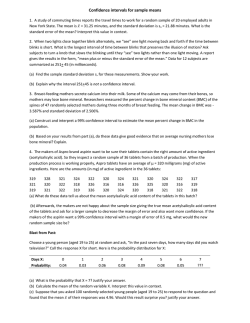
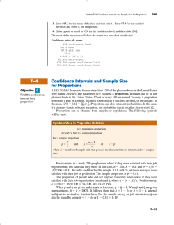
Chapter 5 One- and Two-Sample Estimation Problems 5.1 Introduction In previous chapters, we emphasized sampling properties of the sample mean and variance. We also emphasized displays of data in various forms. The purpose of these presentations is to build a foundation that allows us to draw conclusions about the population parameters from experimental data. For example, the Central Limit ¯ The Theorem provides information about the distribution of the sample mean X. distribution involves the population mean μ. Thus, any conclusions concerning μ drawn from an observed sample average must depend on knowledge of this sampling distribution. Similar comments apply to S 2 and σ 2 . Clearly, any conclusions we draw about the variance of a normal distribution will likely involve the sampling distribution of S 2 . In this chapter, we begin by formally outlining the purpose of statistical inference. We follow this by discussing the problem of estimation of population parameters. We confine our formal developments of specific estimation procedures to problems involving one and two samples. 5.2 Statistical Inference In Chapter 1, we discussed the general philosophy of formal statistical inference. Statistical inference consists of those methods by which one makes inferences or generalizations about a population. The trend today is to distinguish between the classical method of estimating a population parameter, whereby inferences are based strictly on information obtained from a random sample selected from the population, and the Bayesian method, which utilizes prior subjective knowledge about the probability distribution of the unknown parameters in conjunction with the information provided by the sample data. Throughout most of this chapter, we shall use classical methods to estimate unknown population parameters such as the mean, the proportion, and the variance by computing statistics from random 195 196 Chapter 5 One- and Two-Sample Estimation Problems samples and applying the theory of sampling distributions, much of which was covered in Chapter 4. Statistical inference may be divided into two major areas: estimation and tests of hypotheses. We treat these two areas separately, dealing with theory and applications of estimation in this chapter and hypothesis testing in Chapter 6. To distinguish clearly between the two areas, consider the following examples. A candidate for public office may wish to estimate the true proportion of voters favoring him by obtaining opinions from a random sample of 100 eligible voters. The fraction of voters in the sample favoring the candidate could be used as an estimate of the true proportion in the population of voters. A knowledge of the sampling distribution of a proportion enables one to establish the degree of accuracy of such an estimate. This problem falls in the area of estimation. Now consider the case in which one is interested in finding out whether brand A floor wax is more scuff-resistant than brand B floor wax. He or she might hypothesize that brand A is better than brand B and, after proper testing, accept or reject this hypothesis. In this example, we do not attempt to estimate a parameter, but instead we try to arrive at a correct decision about a prestated hypothesis. Once again we are dependent on sampling theory and the use of data to provide us with some measure of accuracy for our decision. 5.3 Classical Methods of Estimation A point estimate of some population parameter θ is a single value θˆ of a statistic ˆ For example, the value x ¯ computed from a sample of size n, �. ¯ of the statistic X, is a point estimate of the population parameter μ. Similarly, pˆ = x/n is a point estimate of the true proportion p for a binomial experiment. An estimator is not expected to estimate the population parameter without ¯ to estimate μ exactly, but we certainly hope that it is error. We do not expect X not far off. For a particular sample, it is possible to obtain a closer estimate of μ ˜ as an estimator. Consider, for instance, a sample by using the sample median X consisting of the values 2, 5, and 11 from a population whose mean is 4 but is supposedly unknown. We would estimate μ to be x ¯ = 6, using the sample mean as our estimate, or x ˜ = 5, using the sample median as our estimate. In this case, ˜ produces an estimate closer to the true parameter than does the the estimator X ¯ estimator X. On the other hand, if our random sample contains the values 2, 6, ¯ is the better estimator. Not knowing the true and 7, then x ¯ = 5 and x ˜ = 6, so X ¯ or X ˜ as our estimator. value of μ, we must decide in advance whether to use X Unbiased Estimator What are the desirable properties of a “good” decision function that would influˆ be an estimator whose ence us to choose one estimator rather than another? Let � value θˆ is a point estimate of some unknown population parameter θ. Certainly, we ˆ to have a mean equal to the parameter would like the sampling distribution of � estimated. An estimator possessing this property is said to be unbiased. 5.3 Classical Methods of Estimation 197 Definition 5.1: A statistic � ˆ is said to be an unbiased estimator of the parameter θ if ˆ μ� ˆ = E(�) = θ. Example 5.1: If a sample X1 , . . . , Xn has an unknown population mean μ, then the sample mean ¯ is an unbiased estimator for μ. X Solution : This result can be easily shown as ¯ =E E(X) 1 n n Xi = i=1 1 n n E(Xi ) = i=1 1 n n μ = μ. i=1 This means that the sample mean is always unbiased to the population mean. Example 5.2: Show that S 2 is an unbiased estimator of the parameter σ 2 . Solution : One can show that (see Exercise 5.10) n n ¯ 2= (Xi − X) i=1 ¯ − μ)2 . (Xi − μ)2 − n(X i=1 Now E(S 2 ) = E = 1 n−1 n ¯ 2 (Xi − X) i=1 n 1 n−1 ¯ − μ)2 = E(Xi − μ)2 − nE(X i=1 1 n−1 n 2 2 σX − nσX ¯ i . i=1 However, 2 2 σX = σ 2 , for i = 1, 2, . . . , n, and σX ¯ = i σ2 . n Therefore, E(S 2 ) = 1 n−1 nσ 2 − n σ2 n = σ2 . This result shows that the sample variance is always unbiased to the population variance σ 2 . Although S 2 is an unbiased estimator of σ 2 , S, on the other hand, is usually a biased estimator of σ, with the bias becoming insignificant for large samples. This example illustrates why we divide by n − 1 rather than n when the variance is estimated. Variance of a Point Estimator ˆ 1 and � ˆ 2 are two unbiased estimators of the same population parameter θ, we If � want to choose the estimator whose sampling distribution has the smaller variance. ˆ 1 is a more efficient estimator of θ than � ˆ 2. Hence, if σθ2ˆ < σθ2ˆ , we say that � 1 2 198 Chapter 5 One- and Two-Sample Estimation Problems Definition 5.2: If we consider all possible unbiased estimators of some parameter θ, the one with the smallest variance is called the most efficient estimator of θ. Figure 5.1 illustrates the sampling distributions of three different estimators, ˆ 1, � ˆ 2 , and � ˆ 3 , all estimating θ. It is clear that only � ˆ 1 and � ˆ 2 are unbiased, � ˆ since their distributions are centered at θ. The estimator �1 has a smaller variance ˆ 2 and is therefore more efficient. Hence, our choice for an estimator of θ, than � ˆ 1. among the three considered, would be � ^ ⌰ 1 ^ ⌰ 3 ^ ⌰ 2 θ ^ θ Figure 5.1: Sampling distributions of different estimators of θ. ¯ and X ˜ are unbiased estimaFor normal populations, one can show that both X ¯ tors of the population mean μ, but the variance of X is smaller than the variance ˜ Thus, both estimates x of X. ¯ and x ˜ will, on average, equal the population mean ¯ is more efficient μ, but x ¯ is likely to be closer to μ for a given sample, and thus X ˜ than X. Interval Estimation Even the most efficient unbiased estimator is unlikely to estimate the population parameter exactly. It is true that estimation accuracy increases with large samples, but there is still no reason we should expect a point estimate from a given sample to be exactly equal to the population parameter it is supposed to estimate. There are many situations in which it is preferable to determine an interval within which we would expect to find the value of the parameter. Such an interval is called an interval estimate. An interval estimate of a population parameter θ is an interval of the form ˆ for a θˆL < θ < θˆU , where θˆL and θˆU depend on the value of the statistic � ˆ particular sample and also on the sampling distribution of �. For example, a random sample of SAT verbal scores for students in the entering freshman class might produce an interval from 530 to 550, within which we expect to find the true average of all SAT verbal scores for the freshman class. The values of the endpoints, 530 and 550, will depend on the computed sample mean x ¯ and the ¯ As the sample size increases, we know that σ 2¯ = σ 2 /n sampling distribution of X. X decreases, and consequently our estimate is likely to be closer to the parameter μ, 5.4 Single Sample: Estimating the Mean 199 resulting in a shorter interval. Thus, the interval estimate indicates, by its length, the accuracy of the point estimate. An engineer will gain some insight into the population proportion defective by taking a sample and computing the sample proportion defective. But an interval estimate might be more informative. Interpretation of Interval Estimates ˆ and, therefore, Since different samples will generally yield different values of � ˆ ˆ different values for θL and θU , these endpoints of the interval are values of correˆ L and � ˆ U . From the sampling distribution of � ˆ we sponding random variables � ˆ ˆ ˆ ˆ shall be able to determine �L and �U such that P (�L < θ < �U ) is equal to any ˆ L and � ˆU positive fractional value we care to specify. If, for instance, we find � such that ˆL < θ < � ˆ U ) = 1 − α, P (� for 0 < α < 1, then we have a probability of 1−α of selecting a random sample that will produce an interval containing θ. The interval θˆL < θ < θˆU , computed from the selected sample, is called a 100(1 − α)% confidence interval, the fraction 1 − α is called the confidence coefficient or the degree of confidence, and the endpoints, θˆL and θˆU , are called the lower and upper confidence limits. Thus, when α = 0.05, we have a 95% confidence interval, and when α = 0.01, we obtain a wider 99% confidence interval. The wider the confidence interval is, the more confident we can be that the interval contains the unknown parameter. Of course, it is better to be 95% confident that the average life of a certain television transistor is between 6 and 7 years than to be 99% confident that it is between 3 and 10 years. Ideally, we prefer a short interval with a high degree of confidence. Sometimes, restrictions on the size of our sample prevent us from achieving short intervals without sacrificing some degree of confidence. In the sections that follow, we pursue the notions of point and interval estimation, with each section presenting a different special case. The reader should notice that while point and interval estimation represent different approaches to gaining information regarding a parameter, they are related in the sense that confidence interval estimators are based on point estimators. In the following section, ¯ is a very reasonable point estimator of μ. As a for example, we will see that X result, the important confidence interval estimator of μ depends on knowledge of ¯ the sampling distribution of X. 5.4 Single Sample: Estimating the Mean ¯ is centered at μ, and in most applications the The sampling distribution of X variance is smaller than that of any other unbiased estimators of μ. Thus, the sample mean x ¯ will be used as a point estimate for the population mean μ. Recall 2 2 ¯ that comes from a that σX = σ /n, so a large sample will yield a value of X ¯ sampling distribution with a small variance. Hence, x ¯ is likely to be a very accurate estimate of μ when n is large. 200 Chapter 5 One- and Two-Sample Estimation Problems Let us now consider the interval estimate of μ. If our sample is selected from a normal population or, failing this, if n is sufficiently large, we can establish a ¯ confidence interval for μ by considering the sampling distribution of X. According to the Central Limit Theorem, we can expect the sampling distribu¯ to be approximately normal with mean μX¯ = μ and standard deviation tion of X √ σX¯ = σ/ n. Writing zα/2 for the z-value above which we find an area of α/2 under the normal curve, we can see from Figure 5.2 that P (−zα/2 < Z < zα/2 ) = 1 − α, where Z= ¯ −μ X √ . σ/ n Hence, P −zα/2 < ¯ −μ X √ < zα/2 σ/ n = 1 − α. 1−α α /2 −zα /2 α /2 zα /2 0 z Figure 5.2: P (−zα/2 < Z < zα/2 ) = 1 − α. √ ¯ from each Multiplying each term in the inequality by σ/ n and then subtracting X term and multiplying by −1 (reversing the sense of the inequalities), we obtain P ¯ − zα/2 √σ < μ < X ¯ + zα/2 √σ X n n = 1 − α. A random sample of size n is selected from a population whose variance σ 2 is known, and the mean x ¯ is computed to give the 100(1 − α)% confidence interval below. It is important to emphasize that we have invoked the Central Limit Theorem above. As a result, it is important to note the conditions for applications that follow. Confidence Interval on μ, σ 2 Known If x ¯ is the mean of a random sample of size n from a population with known variance σ 2 , a 100(1 − α)% confidence interval for μ is given by σ σ ¯ + zα/2 √ , x ¯ − zα/2 √ < μ < x n n where zα/2 is the z-value leaving an area of α/2 to the right. 5.4 Single Sample: Estimating the Mean 201 For small samples selected from nonnormal populations, we cannot expect our degree of confidence to be accurate. However, for samples of size n ≥ 30, with the shape of the distributions not too skewed, sampling theory guarantees good results. ˆ L and � ˆ U , defined in Section 5.3, Clearly, the values of the random variables � are the confidence limits σ σ and θˆU = x θˆL = x ¯ − zα/2 √ ¯ + zα/2 √ . n n Different samples will yield different values of x ¯ and therefore produce different interval estimates of the parameter μ, as shown in Figure 5.3. The dot at the center of each interval indicates the position of the point estimate x ¯ for that random sample. Note that all of these intervals are of the same width, since their widths depend only on the choice of zα/2 once x ¯ is determined. The larger the value we choose for zα/2 , the wider we make all the intervals and the more confident we can be that the particular sample selected will produce an interval that contains the unknown parameter μ. In general, for a selection of zα/2 , 100(1 − α)% of the intervals will cover μ. 10 9 8 Sample 7 6 5 4 3 2 1 μ x Figure 5.3: Interval estimates of μ for different samples. Example 5.3: The average zinc concentration recovered from a sample of measurements taken in 36 different locations in a river is found to be 2.6 grams per milliliter. Find the 95% and 99% confidence intervals for the mean zinc concentration in the river. Assume that the population standard deviation is 0.3 gram per milliliter. Solution : The point estimate of μ is x ¯ = 2.6. The z-value leaving an area of 0.025 to the right, and therefore an area of 0.975 to the left, is z0.025 = 1.96 (Table A.3). Hence, 202 Chapter 5 One- and Two-Sample Estimation Problems the 95% confidence interval is 2.6 − (1.96) 0.3 √ 36 < μ < 2.6 + (1.96) 0.3 √ 36 , which reduces to 2.50 < μ < 2.70. To find a 99% confidence interval, we find the z-value leaving an area of 0.005 to the right and 0.995 to the left. From Table A.3 again, z0.005 = 2.575, and the 99% confidence interval is 2.6 − (2.575) 0.3 √ 36 < μ < 2.6 + (2.575) 0.3 √ 36 , or simply 2.47 < μ < 2.73. We now see that a longer interval is required to estimate μ with a higher degree of confidence. The 100(1−α)% confidence interval provides an estimate of the accuracy of our point estimate. If μ is actually the center value of the interval, then x ¯ estimates μ without error. Most of the time, however, x ¯ will not be exactly equal to μ and the point estimate will be in error. The size of this error will be the absolute value of the difference between μ and x ¯, and we can be 100(1 − α)% confident that this difference will not exceed zα/2 √σn . We can readily see this if we draw a diagram of a hypothetical confidence interval, as in Figure 5.4. Error x Ϫzα /2σ / n x μ x ϩ zα /2 σ / n Figure 5.4: Error in estimating μ by x ¯. ¯ is used as an estimate of μ, we can be 100(1 − α)% confident that the error Theorem 5.1: If x will not exceed zα/2 √σn . In Example 5.3, we are 95% confident that the sample mean x ¯ = 2.6 differs √ from the true mean μ by an amount less than (1.96)(0.3)/ 36 = 0.1 and 99% √ confident that the difference is less than (2.575)(0.3)/ 36 = 0.13. Frequently, we wish to know how large a sample is necessary to ensure that the error in estimating μ will be less than a specified amount e. By Theorem 5.1, we must choose n such that zα/2 √σn = e. Solving this equation gives the following formula for n. 5.4 Single Sample: Estimating the Mean 203 ¯ is used as an estimate of μ, we can be 100(1 − α)% confident that the error Theorem 5.2: If x will not exceed a specified amount e when the sample size is n= zα/2 σ e 2 . When solving for the sample size, n, we round all fractional values up to the next whole number. By adhering to this principle, we can be sure that our degree of confidence never falls below 100(1 − α)%. Strictly speaking, the formula in Theorem 5.2 is applicable only if we know the variance of the population from which we select our sample. Lacking this information, we could take a preliminary sample of size n ≥ 30 to provide an estimate of σ. Then, using s as an approximation for σ in Theorem 5.2, we could determine approximately how many observations are needed to provide the desired degree of accuracy. Example 5.4: How large a sample is required if we want to be 95% confident that our estimate of μ in Example 5.3 is off by less than 0.05? Solution : The population standard deviation is σ = 0.3. Then, by Theorem 5.2, n= (1.96)(0.3) 0.05 2 = 138.3. Therefore, we can be 95% confident that a random sample of size 139 will provide an estimate x ¯ differing from μ by an amount less than 0.05. One-Sided Confidence Bounds The confidence intervals and resulting confidence bounds discussed thus far are two-sided (i.e., both upper and lower bounds are given). However, there are many applications in which only one bound is sought. For example, if the measurement of interest is tensile strength, the engineer receives better information from a lower bound only. This bound communicates the worst-case scenario. On the other hand, if the measurement is something for which a relatively large value of μ is not profitable or desirable, then an upper confidence bound is of interest. An example would be a case in which inferences need to be made concerning the mean mercury concentration in a river. An upper bound is very informative in this case. One-sided confidence bounds are developed in the same fashion as two-sided intervals. However, the source is a one-sided probability statement that makes use of the Central Limit Theorem: P ¯ −μ X √ < zα σ/ n = 1 − α. One can then manipulate the probability statement much as before and obtain √ ¯ − zα σ/ n) = 1 − α. P (μ > X 204 Chapter 5 One- and Two-Sample Estimation Problems Similar manipulation of P ¯ X−μ √ σ/ n > −zα = 1 − α gives √ ¯ + zα σ/ n) = 1 − α. P (μ < X As a result, the upper and lower one-sided bounds follow. One-Sided Confidence Bounds on μ, σ 2 Known ¯ is the mean of a random sample of size n from a population with variance If X σ 2 , the one-sided 100(1 − α)% confidence bounds for μ are given by √ upper one-sided bound: x ¯ + zα σ/ n; √ lower one-sided bound: x ¯ − zα σ/ n. Example 5.5: In a psychological testing experiment, 25 subjects are selected randomly and their reaction time, in seconds, to a particular stimulus is measured. Past experience suggests that the variance in reaction times to these types of stimuli is 4 sec2 and that the distribution of reaction times is approximately normal. The average time for the subjects is 6.2 seconds. Give an upper 95% bound for the mean reaction time. Solution : The upper 95% bound is given by √ x ¯ + zα σ/ n = 6.2 + (1.645) 4/25 = 6.2 + 0.658 = 6.858 seconds. Hence, we are 95% confident that the mean reaction time is less than 6.858 seconds. The Case of σ Unknown Frequently, we must attempt to estimate the mean of a population when the variance is unknown. The reader should recall learning in Chapter 4 that if we have a random sample from a normal distribution, then the random variable T = ¯ −μ X √ S/ n has a Student t-distribution with n − 1 degrees of freedom. Here S is the sample standard deviation. In this situation, with σ unknown, T can be used to construct a confidence interval on μ. The procedure is the same as that with σ known except that σ is replaced by S and the standard normal distribution is replaced by the t-distribution. Referring to Figure 5.5, we can assert that P (−tα/2 < T < tα/2 ) = 1 − α, where tα/2 is the t-value with n−1 degrees of freedom, above which we find an area of α/2. Because of symmetry, an equal area of α/2 will fall to the left of −tα/2 . Substituting for T , we write P −tα/2 < ¯ −μ X √ < tα/2 S/ n = 1 − α. 5.4 Single Sample: Estimating the Mean 205 √ ¯ from Multiplying each term in the inequality by S/ n, and then subtracting X each term and multiplying by −1, we obtain ¯ − tα/2 √S < μ < X ¯ + tα/2 √S = 1 − α. X n n For a particular random sample of size n, the mean x ¯ and standard deviation s are computed and the following 100(1 − α)% confidence interval for μ is obtained. P 1 −α α /2 −t α 2 0 α /2 tα 2 t Figure 5.5: P (−tα/2 < T < tα/2 ) = 1 − α. Confidence Interval on μ, σ 2 Unknown If x ¯ and s are the mean and standard deviation of a random sample from a normal population with unknown variance σ 2 , a 100(1 − α)% confidence interval for μ is s s x ¯ − tα/2 √ < μ < x ¯ + tα/2 √ , n n where tα/2 is the t-value with v = n − 1 degrees of freedom, leaving an area of α/2 to the right. We have made a distinction between the cases of σ known and σ unknown in computing confidence interval estimates. We should emphasize that for σ known we exploited the Central Limit Theorem, whereas for σ unknown we made use of the sampling distribution of the random variable T . However, the use of the tdistribution is based on the premise that the sampling is from a normal distribution. As long as the distribution is approximately bell shaped, confidence intervals can be computed when σ 2 is unknown by using the t-distribution and we may expect very good results. Computed one-sided confidence bounds for μ with σ unknown are as the reader would expect, namely s s x ¯ + tα √ and x ¯ − tα √ . n n They are the upper and lower 100(1 − α)% bounds, respectively. Here tα is the t-value having an area of α to the right. Example 5.6: The contents of seven similar containers of sulfuric acid are 9.8, 10.2, 10.4, 9.8, 10.0, 10.2, and 9.6 liters. Find a 95% confidence interval for the mean contents of all such containers, assuming an approximately normal distribution. 206 Chapter 5 One- and Two-Sample Estimation Problems Solution : The sample mean and standard deviation for the given data are x ¯ = 10.0 and s = 0.283. Using Table A.4, we find t0.025 = 2.447 for v = 6 degrees of freedom. Hence, the 95% confidence interval for μ is 10.0 − (2.447) 0.283 √ 7 < μ < 10.0 + (2.447) 0.283 √ 7 , which reduces to 9.74 < μ < 10.26. Concept of a Large-Sample Confidence Interval Often statisticians recommend that even when normality cannot be assumed, σ is unknown, and n ≥ 30, s can replace σ and the confidence interval s x ¯ ± zα/2 √ n may be used. This is often referred to as a large-sample confidence interval. The justification lies only in the presumption that with a sample as large as 30 and the population distribution not too skewed, s will be very close to the true σ and thus the Central Limit Theorem prevails. It should be emphasized that this is only an approximation and the quality of the result becomes better as the sample size grows larger. Example 5.7: Scholastic Aptitude Test (SAT) mathematics scores of a random sample of 500 high school seniors in the state of Texas are collected, and the sample mean and standard deviation are found to be 501 and 112, respectively. Find a 99% confidence interval on the mean SAT mathematics score for seniors in the state of Texas. Solution : Since the sample size is large, it is reasonable to use the normal approximation. Using Table A.3, we find z0.005 = 2.575. Hence, a 99% confidence interval for μ is 501 ± (2.575) 112 √ 500 = 501 ± 12.9, which yields 488.1 < μ < 513.9. 5.5 Standard Error of a Point Estimate We have made a rather sharp distinction between the goal of a point estimate and that of a confidence interval estimate. The former supplies a single number extracted from a set of experimental data, and the latter provides an interval that is reasonable for the parameter, given the experimental data; that is, 100(1 − α)% of such computed intervals “cover” the parameter. These two approaches to estimation are related to each other. The common thread is the sampling distribution of the point estimator. Consider, for example, 5.6 Prediction Intervals 207 ¯ of μ with σ known. We indicated earlier that a measure of the the estimator X ¯ is quality of an unbiased estimator is its variance. The variance of X 2 σX ¯ = σ2 . n ¯ or standard error of X, ¯ is σ/√n. Simply put, Thus, the standard deviation of X, ¯ the computed the standard error of an estimator is its standard deviation. For X, confidence limit σ x ¯ ± zα/2 √ is written as x ¯ ± zα/2 s.e.(¯ x), n where “s.e.” is the “standard error.” The important point is that the width of the confidence interval on μ is dependent on the quality of the point estimator through its standard error. In the case where σ is unknown and sampling √ is from a normal distribution, s replaces σ and the estimated standard error s/ n is involved. Thus, the confidence limits on μ are as follows. Confidence Limits on μ, σ 2 Unknown s x ¯ ± tα/2 √ = x ¯ ± tα/2 s.e.(¯ x) n Again, the confidence interval is no better (in terms of width) than the quality of the point estimate, in this case through its estimated standard error. Computer packages often refer to estimated standard errors simply as “standard errors.” As we move to more complex confidence intervals, there is a prevailing notion that widths of confidence intervals become shorter as the quality of the corresponding point estimate becomes better, although it is not always quite as simple as we have illustrated here. It can be argued that a confidence interval is merely an augmentation of the point estimate to take into account the precision of the point estimate. 5.6 Prediction Intervals The point and interval estimations of the mean in Sections 5.4 and 5.5 provide good information about the unknown parameter μ of a normal distribution or a nonnormal distribution from which a large sample is drawn. Sometimes, other than the population mean, the experimenter may also be interested in predicting the possible value of a future observation. For instance, in quality control, the experimenter may need to use the observed data to predict a new observation. A process that produces a metal part may be evaluated on the basis of whether the part meets specifications on tensile strength. On certain occasions, a customer may be interested in purchasing a single part. In this case, a confidence interval on the mean tensile strength does not capture the required information. The customer requires a statement regarding the uncertainty of a single observation. This type of requirement is nicely fulfilled by the construction of a prediction interval. It is quite simple to obtain a prediction interval for the situations we have considered so far. Assume that the random sample comes from a normal population with unknown mean μ and known variance σ 2 . A natural point estimator of a 208 Chapter 5 One- and Two-Sample Estimation Problems ¯ It is known, from Section 4.4, that the variance of X ¯ is new observation is X. σ 2 /n. However, to predict a new observation, not only do we need to account for the variation due to estimating the mean, but also we should account for the variation of a future observation. From the assumption, we know that the variance of the random error in a new observation is σ 2 . The development of a prediction interval is best illustrated by beginning with a normal random variable x0 − x ¯, where x0 is the new observation and x ¯ comes from the sample. Since x0 and x ¯ are independent, we know that z= ¯ x0 − x σ2 + σ 2 /n = x0 − x ¯ σ 1 + 1/n is n(z; 0, 1). As a result, if we use the probability statement P (−zα/2 < Z < zα/2 ) = 1 − α with the z-statistic above and place x0 in the center of the probability statement, we have the following event occurring with probability 1 − α: x ¯ − zα/2 σ 1 + 1/n < x0 < x ¯ + zα/2 σ 1 + 1/n. Computation of the prediction interval is formalized as follows. Prediction Interval of a Future Observation, σ 2 Known For a normal distribution of measurements with unknown mean μ and known variance σ 2 , a 100(1 − α)% prediction interval of a future observation x0 is x ¯ − zα/2 σ 1 + 1/n < x0 < x ¯ + zα/2 σ 1 + 1/n, where zα/2 is the z-value leaving an area of α/2 to the right. Example 5.8: Due to the decrease in interest rates, the First Citizens Bank received a lot of mortgage applications. A recent sample of 50 mortgage loans resulted in an average loan amount of $257,300. Assume a population standard deviation of $25,000. For the next customer who fills out a mortgage application, find a 95% prediction interval for the loan amount. Solution : The point prediction of the next customer’s loan amount is x ¯ = $257,300. The z-value here is z0.025 = 1.96. Hence, a 95% prediction interval for the future loan amount is 257,300 − (1.96)(25,000) 1 + 1/50 < x0 < 257,300 + (1.96)(25,000) 1 + 1/50, which gives the interval ($207,812.43, $306,787.57). The prediction interval provides a good estimate of the location of a future observation, which is quite different from the estimate of the sample mean value. It should be noted that the variation of this prediction is the sum of the variation due to an estimation of the mean and the variation of a single observation. However, as in the past, we first consider the case with known variance. It is also important to deal with the prediction interval of a future observation in the situation where the variance is unknown. Indeed a Student t-distribution may be used in this case, as described in the following result. The normal distribution is merely replaced by the t-distribution. 5.6 Prediction Intervals Prediction Interval of a Future Observation, σ 2 Unknown 209 For a normal distribution of measurements with unknown mean μ and unknown variance σ 2 , a 100(1 − α)% prediction interval of a future observation x0 is x ¯ − tα/2 s 1 + 1/n < x0 < x ¯ + tα/2 s 1 + 1/n, where tα/2 is the t-value with v = n − 1 degrees of freedom, leaving an area of α/2 to the right. One-sided prediction intervals can also be constructed. Upper prediction bounds apply in cases where focus must be placed on future large observations. Concern over future small observations calls for the use of lower prediction bounds. The upper bound is given by x ¯ + tα s 1 + 1/n x ¯ − tα s 1 + 1/n. and the lower bound by Example 5.9: A meat inspector has randomly selected 30 packs of 95% lean beef. The sample resulted in a mean of 96.2% with a sample standard deviation of 0.8%. Find a 99% prediction interval for the leanness of a new pack. Assume normality. Solution : For v = 29 degrees of freedom, t0.005 = 2.756. Hence, a 99% prediction interval for a new observation x0 is 96.2 − (2.756)(0.8) 1+ 1 < x0 < 96.2 + (2.756)(0.8) 30 1+ 1 , 30 which reduces to (93.96, 98.44). Use of Prediction Limits for Outlier Detection To this point in the text very little attention has been paid to the concept of outliers, or aberrant observations. The majority of scientific investigators are keenly sensitive to the existence of outlying observations or so-called faulty or “bad” data. It is certainly of interest here since there is an important relationship between outlier detection and prediction intervals. It is convenient for our purposes to view an outlying observation as one that comes from a population with a mean that is different from the mean that governs the rest of the sample of size n being studied. The prediction interval produces a bound that “covers” a future single observation with probability 1 − α if it comes from the population from which the sample was drawn. As a result, a methodology for outlier detection involves the rule that an observation is an outlier if it falls outside the prediction interval computed without including the questionable observation in the sample. As a result, for the prediction interval of Example 5.9, if a new pack of beef is measured and its leanness is outside the interval (93.96, 98.44), that observation can be viewed as an outlier. 210 5.7 Chapter 5 One- and Two-Sample Estimation Problems Tolerance Limits As discussed in Section 5.6, the scientist or engineer may be less interested in estimating parameters than in gaining a notion about where an individual observation or measurement might fall. Such situations call for the use of prediction intervals. However, there is yet a third type of interval that is of interest in many applications. Once again, suppose that interest centers around the manufacturing of a component part and specifications exist on a dimension of that part. In addition, there is little concern about the mean of the dimension. But unlike in the scenario in Section 5.6, one may be less interested in a single observation and more interested in where the majority of the population falls. If process specifications are important, the manager of the process is concerned about long-range performance, not the next observation. One must attempt to determine bounds that, in some probabilistic sense, “cover” values in the population (i.e., the measured values of the dimension). One method of establishing the desired bounds is to determine a confidence interval on a fixed proportion of the measurements. This is best motivated by visualizing a situation in which we are doing random sampling from a normal distribution with known mean μ and variance σ 2 . Clearly, a bound that covers the middle 95% of the population of observations is μ ± 1.96σ. This is called a tolerance interval, and indeed its coverage of 95% of measured observations is exact. However, in practice, μ and σ are seldom known; thus, the user must apply x ¯ ± ks. Now, of course, the interval is a random variable, and hence the coverage of a proportion of the population by the interval is not exact. As a result, a 100(1−γ)% confidence interval must be used since x ¯ ± ks cannot be expected to cover any specified proportion all the time. As a result, we have the following definition. Tolerance Limits For a normal distribution of measurements with unknown mean μ and unknown standard deviation σ, tolerance limits are given by x ¯ ± ks, where k is determined such that one can assert with 100(1 − γ)% confidence that the given limits contain at least the proportion 1 − α of the measurements. Table A.7 gives values of k for 1 − α = 0.90, 0.95, 0.99; γ = 0.05, 0.01; and selected values of n from 2 to 300. Example 5.10: Consider Example 5.9. With the information given, find a tolerance interval that gives two-sided 95% bounds on 90% of the distribution of packages of 95% lean beef. Assume the data came from an approximately normal distribution. Solution : Recall from Example 5.9 that n = 30, the sample mean is 96.2%, and the sample standard deviation is 0.8%. From Table A.7, k = 2.14. Using x ¯ ± ks = 96.2 ± (2.14)(0.8), 5.7 Tolerance Limits 211 we find that the lower and upper bounds are 94.5 and 97.9. We are 95% confident that the above range covers the central 90% of the distribution of 95% lean beef packages. Distinction among Confidence Intervals, Prediction Intervals, and Tolerance Intervals It is important to reemphasize the difference among the three types of intervals discussed and illustrated in the preceding sections. The computations are straightforward, but interpretation can be confusing. In real-life applications, these intervals are not interchangeable because their interpretations are quite distinct. In the case of confidence intervals, one is attentive only to the population mean. For example, Exercise 5.11 on page 213 deals with an engineering process that produces shearing pins. A specification will be set on Rockwell hardness, below which a customer will not accept any pins. Here, a population parameter must take a backseat. It is important that the engineer know where the majority of the values of Rockwell hardness are going to be. Thus, tolerance limits should be used. Surely, when tolerance limits on any process output are tighter than process specifications, that is good news for the process manager. It is true that the tolerance limit interpretation is somewhat related to the confidence interval. The 100(1−α)% tolerance interval on, say, the proportion 0.95 can be viewed as a confidence interval on the middle 95% of the corresponding normal distribution. One-sided tolerance limits are also relevant. In the case of the Rockwell hardness problem, it is desirable to have a lower bound of the form x ¯ − ks such that there is 99% confidence that at least 99% of Rockwell hardness values will exceed the computed value. Prediction intervals are applicable when it is important to determine a bound on a single value. The mean is not the issue here, nor is the location of the majority of the population. Rather, the location of a single new observation is required. Case Study 5.1: Machine Quality: A machine produces metal pieces that are cylindrical in shape. A sample of these pieces is taken, and the diameters are found to be 1.01, 0.97, 1.03, 1.04, 0.99, 0.98, 0.99, 1.01, and 1.03 centimeters. Use these data to calculate three interval types and draw interpretations that illustrate the distinction between them in the context of the system. For all computations, assume an approximately normal distribution. The sample mean and standard deviation for the given data are x ¯ = 1.0056 and s = 0.0246. (a) Find a 99% confidence interval on the mean diameter. (b) Compute a 99% prediction interval on a measured diameter of a single metal piece taken from the machine. (c) Find the 99% tolerance limits that will contain 95% of the metal pieces produced by this machine. Solution : (a) The 99% confidence interval for the mean diameter is given by √ x ¯ ± t0.005 s/ n = 1.0056 ± (3.355)(0.0246/3) = 1.0056 ± 0.0275. 212 Chapter 5 One- and Two-Sample Estimation Problems Thus, the 99% confidence bounds are 0.9781 and 1.0331. (b) The 99% prediction interval for a future observation is given by x ¯ ± t0.005 s 1 + 1/n = 1.0056 ± (3.355)(0.0246) 1 + 1/9, with the bounds being 0.9186 and 1.0926. (c) From Table A.7, for n = 9, 1 − γ = 0.99, and 1 − α = 0.95, we find k = 4.550 for two-sided limits. Hence, the 99% tolerance limits are given by x ¯ + ks = 1.0056 ± (4.550)(0.0246), with the bounds being 0.8937 and 1.1175. We are 99% confident that the tolerance interval from 0.8937 to 1.1175 will contain the central 95% of the distribution of diameters produced. This case study illustrates that the three types of limits can give appreciably different results even though they are all 99% bounds. In the case of the confidence interval on the mean, 99% of such intervals cover the population mean diameter. Thus, we say that we are 99% confident that the mean diameter produced by the process is between 0.9781 and 1.0331 centimeters. Emphasis is placed on the mean, with less concern about a single reading or the general nature of the distribution of diameters in the population. In the case of the prediction limits, the bounds 0.9186 and 1.0926 are based on the distribution of a single “new” metal piece taken from the process, and again 99% of such limits will cover the diameter of a new measured piece. On the other hand, the tolerance limits, as suggested in the previous section, give the engineer a sense of where the “majority,” say the central 95%, of the diameters of measured pieces in the population reside. The 99% tolerance limits, 0.8937 and 1.1175, are numerically quite different from the other two bounds. If these bounds appear alarmingly wide to the engineer, it reflects negatively on process quality. On the other hand, if the bounds represent a desirable result, the engineer may conclude that a majority (95% in this case) of the diameters are in a desirable range. Again, a confidence interval interpretation may be used: namely, 99% of such calculated bounds will cover the middle 95% of the population of diameters. Exercises 5.1 A UCLA researcher claims that the life span of mice can be extended by as much as 25% when the calories in their diet are reduced by approximately 40% from the time they are weaned. The restricted diet is enriched to normal levels by vitamins and protein. Assuming that it is known from previous studies that σ = 5.8 months, how many mice should be included in our sample if we wish to be 99% confident that the mean life span of the sample will be within 2 months of the population mean for all mice subjected to this reduced diet? 5.2 An electrical firm manufactures light bulbs that have a length of life that is approximately normally distributed with a standard deviation of 40 hours. If a sample of 30 bulbs has an average life of 780 hours, find a 96% confidence interval for the population mean of all bulbs produced by this firm. 5.3 Many cardiac patients wear an implanted pacemaker to control their heartbeat. A plastic connector module mounts on the top of the pacemaker. Assuming a standard deviation of 0.0015 inch and an approximately normal distribution, find a 95% confidence Exercises interval for the mean of the depths of all connector modules made by a certain manufacturing company. A random sample of 75 modules has an average depth of 0.310 inch. 213 5.10 For a random sample X1 , . . . , Xn , show that n n i=1 5.4 The heights of a random sample of 50 college students showed a mean of 174.5 centimeters and a standard deviation of 6.9 centimeters. (a) Construct a 98% confidence interval for the mean height of all college students. (b) What can we assert with 98% confidence about the possible size of our error if we estimate the mean height of all college students to be 174.5 centimeters? 5.5 A random sample of 100 automobile owners in the state of Virginia shows that an automobile is driven on average 23,500 kilometers per year with a standard deviation of 3900 kilometers. Assume the distribution of measurements to be approximately normal. (a) Construct a 99% confidence interval for the average number of kilometers an automobile is driven annually in Virginia. (b) What can we assert with 99% confidence about the possible size of our error if we estimate the average number of kilometers driven by car owners in Virginia to be 23,500 kilometers per year? 5.6 How large a sample is needed in Exercise 5.2 if we wish to be 96% confident that our sample mean will be within 10 hours of the true mean? 5.7 How large a sample is needed in Exercise 5.3 if we wish to be 95% confident that our sample mean will be within 0.0005 inch of the true mean? 5.8 An efficiency expert wishes to determine the average time that it takes to drill three holes in a certain metal clamp. How large a sample will she need to be 95% confident that her sample mean will be within 15 seconds of the true mean? Assume that it is known from previous studies that σ = 40 seconds. 5.9 Regular consumption of presweetened cereals contributes to tooth decay, heart disease, and other degenerative diseases, according to studies conducted by Dr. W. H. Bowen of the National Institute of Health and Dr. J. Yudben, Professor of Nutrition and Dietetics at the University of London. In a random sample consisting of 20 similar single servings of Alpha-Bits, the average sugar content was 11.3 grams with a standard deviation of 2.45 grams. Assuming that the sugar contents are normally distributed, construct a 95% confidence interval for the mean sugar content for single servings of Alpha-Bits. ¯ 2 + n(X ¯ − μ)2 . (Xi − X) (Xi − μ)2 = i=1 5.11 A random sample of 12 shearing pins is taken in a study of the Rockwell hardness of the pin head. Measurements on the Rockwell hardness are made for each of the 12, yielding an average value of 48.50 with a sample standard deviation of 1.5. Assuming the measurements to be normally distributed, construct a 90% confidence interval for the mean Rockwell hardness. 5.12 The following measurements were recorded for the drying time, in hours, of a certain brand of latex paint: 3.4 2.8 4.4 2.5 3.3 4.0 4.8 5.6 5.2 2.9 3.7 3.0 3.6 2.8 4.8 Assuming that the measurements represent a random sample from a normal population, find a 95% prediction interval for the drying time for the next trial of the paint. 5.13 Referring to Exercise 5.5, construct a 99% prediction interval for the kilometers traveled annually by an automobile owner in Virginia. 5.14 Consider Exercise 5.9. Compute a 95% prediction interval for the sugar content of the next single serving of Alpha-Bits. 5.15 A random sample of 25 tablets of buffered aspirin contains, on average, 325.05 mg of aspirin per tablet, with a standard deviation of 0.5 mg. Find the 95% tolerance limits that will contain 90% of the tablet contents for this brand of buffered aspirin. Assume that the aspirin content is normally distributed. 5.16 Referring to Exercise 5.11, construct a 95% tolerance interval containing 90% of the measurements. 5.17 In a study conducted by the Zoology department at Virginia Tech, fifteen samples of water were collected from a certain station in the James River in order to gain some insight regarding the amount of orthophosphorus in the river. The concentration of the chemical is measured in milligrams per liter. Let us suppose that the mean at the station is not as important as the upper extreme of the distribution of the concentration of the chemical at the station. Concern centers around whether the concentration at the extreme is too large. Readings for the fifteen water samples gave a sample mean of 3.84 milligrams per liter and a sample standard deviation of 3.07 milligrams per liter. Assume 214 Chapter 5 One- and Two-Sample Estimation Problems that the readings are a random sample from a normal distribution. Calculate a prediction interval (upper 95% prediction limit) and a tolerance limit (95% upper tolerance limit that exceeds 95% of the population of values). Interpret both; that is, tell what each communicates about the upper extreme of the distribution of orthophosphorus at the sampling station. 5.18 Consider the situation of Case Study 5.1 on page 211. Estimation of the mean diameter, while important, is not nearly as important as trying to pin down the location of the majority of the distribution of diameters. Find the 95% tolerance limits that contain 95% of the diameters. 5.19 Consider the situation of Case Study 5.1 with a larger sample of metal pieces. The diameters are as follows: 1.01, 0.97, 1.03, 1.04, 0.99, 0.98, 1.01, 1.03, 0.99, 1.00, 1.00, 0.99, 0.98, 1.01, 1.02, 0.99 centimeters. Once again the normality assumption may be made. Do the following and compare your results to those of the case study. Discuss how they are different and why. (a) Compute a 99% confidence interval on the mean diameter. (b) Compute a 99% prediction interval on the next diameter to be measured. (c) Compute a 99% tolerance interval for coverage of the central 95% of the distribution of diameters. 5.20 A type of thread is being studied for its tensile strength properties. Fifty pieces were tested under similar conditions, and the results showed an average 5.8 tensile strength of 78.3 kilograms and a standard deviation of 5.6 kilograms. Assuming a normal distribution of tensile strengths, give a lower 95% prediction limit on a single observed tensile strength value. In addition, give a lower 95% tolerance limit that is exceeded by 99% of the tensile strength values. 5.21 Refer to Exercise 5.20. Why are the quantities requested in the exercise likely to be more important to the manufacturer of the thread than, say, a confidence interval on the mean tensile strength? 5.22 Refer to Exercise 5.20 again. Suppose that specifications by a buyer of the thread are that the tensile strength of the material must be at least 62 kilograms. The manufacturer is satisfied if at most 5% of the manufactured pieces have tensile strength less than 62 kilograms. Is there cause for concern? Use a one-sided 99% tolerance limit that is exceeded by 95% of the tensile strength values. 5.23 Consider the drying time measurements in Exercise 5.12. Suppose the 15 observations in the data set are supplemented by a 16th value of 6.9 hours. In the context of the original 15 observations, is the 16th value an outlier? Show work. 5.24 Consider the data in Exercise 5.11. Suppose the manufacturer of the shearing pins insists that the Rockwell hardness of the product be less than or equal to 44.0 only 5% of the time. What is your reaction? Use a tolerance limit calculation as the basis for your judgment. Two Samples: Estimating the Difference between Two Means If we have two populations with means μ1 and μ2 and variances σ12 and σ22 , respectively, a point estimator of the difference between μ1 and μ2 is given by the ¯1 − X ¯ 2 . Therefore, to obtain a point estimate of μ1 − μ2 , we shall select statistic X two independent random samples, one from each population, of sizes n1 and n2 , and compute x ¯1 − x ¯2 , the difference of the sample means. Clearly, we must consider ¯1 − X ¯2. the sampling distribution of X ¯1 − X ¯2 According to Theorem 4.3, we can expect the sampling distribution of X to be approximately normal with mean μX¯ 1 −X¯ 2 = μ1 − μ2 and standard deviation σX¯ 1 −X¯ 2 = σ12 /n1 + σ22 /n2 . Therefore, we can assert with a probability of 1 − α that the standard normal variable Z= ¯1 − X ¯ 2 ) − (μ1 − μ2 ) (X σ12 /n1 + σ22 /n2 5.8 Two Samples: Estimating the Difference between Two Means 215 will fall between −zα/2 and zα/2 . Referring once again to Figure 5.2 on page 200, we write P (−zα/2 < Z < zα/2 ) = 1 − α. Substituting for Z, we state equivalently that P −zα/2 < ¯ 2 ) − (μ1 − μ2 ) ¯1 − X (X σ12 /n1 + σ22 /n2 < zα/2 = 1 − α, which leads to the following 100(1 − α)% confidence interval for μ1 − μ2 . Confidence Interval for μ1 − μ2 , σ12 and σ22 Known ¯2 are means of independent random samples of sizes n1 and n2 If x ¯1 and x from populations with known variances σ12 and σ22 , respectively, a 100(1 − α)% confidence interval for μ1 − μ2 is given by (¯ x1 − x ¯2 ) − zα/2 σ12 σ2 + 2 < μ1 − μ2 < (¯ x1 − x ¯2 ) + zα/2 n1 n2 σ12 σ2 + 2, n1 n2 where zα/2 is the z-value leaving an area of α/2 to the right. The degree of confidence is exact when samples are selected from normal populations. For nonnormal populations, the Central Limit Theorem allows for a good approximation for reasonable size samples. Variances Unknown but Equal Consider the case where σ12 and σ22 are unknown. If σ12 = σ22 = σ 2 , we obtain a standard normal variable of the form Z= ¯1 − X ¯ 2 ) − (μ1 − μ2 ) (X σ 2 [(1/n1 ) + (1/n2 )] . According to Theorem 4.4, the two random variables (n1 − 1)S12 σ2 and (n2 − 1)S22 σ2 have chi-squared distributions with n1 − 1 and n2 − 1 degrees of freedom, respectively. Furthermore, they are independent chi-squared variables, since the random samples were selected independently. Consequently, their sum V = (n1 − 1)S12 (n2 − 1)S22 (n1 − 1)S12 + (n2 − 1)S22 + = 2 2 σ σ σ2 has a chi-squared distribution with v = n1 + n2 − 2 degrees of freedom. Since the preceding expressions for Z and V can be shown to be independent, it follows from Theorem 4.5 that the statistic T = ¯1 − X ¯ 2 ) − (μ1 − μ2 ) (X σ 2 [(1/n1 ) + (1/n2 )] (n1 − 1)S12 + (n2 − 1)S22 σ 2 (n1 + n2 − 2) 216 Chapter 5 One- and Two-Sample Estimation Problems has the t-distribution with v = n1 + n2 − 2 degrees of freedom. A point estimate of the unknown common variance σ 2 can be obtained by pooling the sample variances. Denoting the pooled estimator by Sp2 , we have the following. Pooled Estimate of Variance Sp2 = (n1 − 1)S12 + (n2 − 1)S22 n1 + n2 − 2 Substituting Sp2 in the T statistic, we obtain the less cumbersome form T = ¯1 − X ¯ 2 ) − (μ1 − μ2 ) (X Sp (1/n1 ) + (1/n2 ) . Using the T statistic, we have P (−tα/2 < T < tα/2 ) = 1 − α, where tα/2 is the t-value with n1 + n2 − 2 degrees of freedom, above which we find an area of α/2. Substituting for T in the inequality, we write P −tα/2 < ¯ 2 ) − (μ1 − μ2 ) ¯1 − X (X Sp (1/n1 ) + (1/n2 ) < tα/2 = 1 − α. After the usual mathematical manipulations, the difference of the sample means x ¯1 − x ¯2 and the pooled variance are computed and then the following 100(1 − α)% confidence interval for μ1 − μ2 is obtained. The value of s2p is easily seen to be a weighted average of the two sample variances s21 and s22 , where the weights are the degrees of freedom. Confidence Interval for μ1 − μ2 , σ12 = σ22 but Both Unknown If x ¯1 and x ¯2 are the means of independent random samples of sizes n1 and n2 , respectively, from approximately normal populations with unknown but equal variances, a 100(1 − α)% confidence interval for μ1 − μ2 is given by (¯ x1 − x ¯2 ) − tα/2 sp 1 1 + < μ1 − μ2 < (¯ x1 − x ¯2 ) + tα/2 sp n1 n2 1 1 + , n1 n2 where sp is the pooled estimate of the population standard deviation and tα/2 is the t-value with v = n1 + n2 − 2 degrees of freedom, leaving an area of α/2 to the right. Example 5.11: The article “Macroinvertebrate Community Structure as an Indicator of Acid Mine Pollution,” published in the Journal of Environmental Pollution, reports on an investigation undertaken in Cane Creek, Alabama, to determine the relationship between selected physiochemical parameters and different measures of macroinvertebrate community structure. One facet of the investigation was an evaluation of the effectiveness of a numerical species diversity index to indicate aquatic degradation due to acid mine drainage. Conceptually, a high index of macroinvertebrate species diversity should indicate an unstressed aquatic system, while a low diversity index should indicate a stressed aquatic system. 5.8 Two Samples: Estimating the Difference between Two Means 217 Two independent sampling stations were chosen for this study, one located downstream from the acid mine discharge point and the other located upstream. For 12 monthly samples collected at the downstream station, the species diversity index had a mean value x ¯1 = 3.11 and a standard deviation s1 = 0.771, while 10 monthly samples collected at the upstream station had a mean index value x ¯2 = 2.04 and a standard deviation s2 = 0.448. Find a 90% confidence interval for the difference between the population means for the two locations, assuming that the populations are approximately normally distributed with equal variances. Solution : Let μ1 and μ2 represent the population means, respectively, for the species diversity indices at the downstream and upstream stations. We wish to find a 90% confidence interval for μ1 − μ2 . Our point estimate of μ1 − μ2 is ¯2 = 3.11 − 2.04 = 1.07. x ¯1 − x The pooled estimate, s2p , of the common variance, σ 2 , is s2p = (n1 − 1)s21 + (n2 − 1)s22 (11)(0.7712 ) + (9)(0.4482 ) = = 0.417. n1 + n2 − 2 12 + 10 − 2 Taking the square root, we obtain sp = 0.646. Using α = 0.1, we find in Table A.4 that t0.05 = 1.725 for v = n1 + n2 − 2 = 20 degrees of freedom. Therefore, the 90% confidence interval for μ1 − μ2 is 1 1 + < μ1 − μ2 < 1.07 + (1.725)(0.646) 12 10 1.07 − (1.725)(0.646) 1 1 + , 12 10 which simplifies to 0.593 < μ1 − μ2 < 1.547. Unknown and Unequal Variances Let us now consider the problem of finding an interval estimate of μ1 − μ2 when the unknown population variances are not likely to be equal. The statistic most often used in this case is ¯ 2 ) − (μ1 − μ2 ) ¯1 − X (X T = , (S12 /n1 ) + (S22 /n2 ) which has approximately a t-distribution with v degrees of freedom, where v= (s21 /n1 + s22 /n2 )2 . − 1)] + [(s22 /n2 )2 /(n2 − 1)] [(s21 /n1 )2 /(n1 Since v is seldom an integer, we round it down to the nearest whole number. The above estimate of the degrees of freedom is called the Satterthwaite approximation (Satterthwaite, 1946, in the Bibliography). Using the statistic T , we write P (−tα/2 < T < tα/2 ) ≈ 1 − α, where tα/2 is the value of the t-distribution with v degrees of freedom, above which we find an area of α/2. Substituting for T in the inequality and following the same steps as before, we state the final result. 218 Confidence Interval for μ1 − μ2 , σ12 = σ22 and Both Unknown Chapter 5 One- and Two-Sample Estimation Problems If x ¯1 and s21 and x ¯2 and s22 are the means and variances of independent random samples of sizes n1 and n2 , respectively, from approximately normal populations with unknown and unequal variances, an approximate 100(1 − α)% confidence interval for μ1 − μ2 is given by (¯ x1 − x ¯2 ) − tα/2 s21 s2 + 2 < μ1 − μ2 < (¯ x1 − x ¯2 ) + tα/2 n1 n2 s21 s2 + 2, n1 n2 where tα/2 is the t-value with v= (s21 /n1 + s22 /n2 )2 [(s21 /n1 )2 /(n1 − 1)] + [(s22 /n2 )2 /(n2 − 1)] degrees of freedom, leaving an area of α/2 to the right. Note that the expression for v above involves random variables, and thus v is an estimate of the degrees of freedom. In applications, this estimate will not result in a whole number, and thus the analyst must round down to the nearest integer to achieve the desired confidence. Before we illustrate the above confidence interval with an example, we should point out that all the confidence intervals on μ1 − μ2 are of the same general form as those on a single mean; namely, they can be written as point estimate ± tα/2 s.e.(point estimate) or point estimate ± zα/2 s.e.(point estimate). For example, in the case where σ1 = σ2 = σ, the estimated standard error of x ¯1 − x ¯2 is sp 1/n1 + 1/n2 . For the case where σ12 = σ22 , ¯2 ) = s.e.(¯ x1 − x s21 s2 + 2. n1 n2 Example 5.12: A study was conducted by the Department of Zoology at Virginia Tech to estimate the difference in the amounts of the chemical orthophosphorus measured at two different stations on the James River. Orthophosphorus was measured in milligrams per liter. Fifteen samples were collected from station 1, and 12 samples were obtained from station 2. The 15 samples from station 1 had an average orthophosphorus content of 3.84 milligrams per liter and a standard deviation of 3.07 milligrams per liter, while the 12 samples from station 2 had an average content of 1.49 milligrams per liter and a standard deviation of 0.80 milligram per liter. Find a 95% confidence interval for the difference in the true average orthophosphorus contents at these two stations, assuming that the observations came from normal populations with different variances. Solution : For station 1, we have x ¯1 = 3.84, s1 = 3.07, and n1 = 15. For station 2, x ¯2 = 1.49, s2 = 0.80, and n2 = 12. We wish to find a 95% confidence interval for μ1 − μ2 . 5.9 Paired Observations 219 Since the population variances are assumed to be unequal, we can only find an approximate 95% confidence interval based on the t-distribution with v degrees of freedom, where v= (3.072 /15 + 0.802 /12)2 = 16.3 ≈ 16. [(3.072 /15)2 /14] + [(0.802 /12)2 /11] Our point estimate of μ1 − μ2 is x ¯1 − x ¯2 = 3.84 − 1.49 = 2.35. Using α = 0.05, we find in Table A.4 that t0.025 = 2.120 for v = 16 degrees of freedom. Therefore, the 95% confidence interval for μ1 − μ2 is 2.35 − 2.120 3.072 0.802 + < μ1 − μ2 < 2.35 + 2.120 15 12 3.072 0.802 + , 15 12 which simplifies to 0.60 < μ1 − μ2 < 4.10. Hence, we are 95% confident that the interval from 0.60 to 4.10 milligrams per liter contains the difference of the true average orthophosphorus contents for these two locations. When two population variances are unknown, the assumption of equal variances or unequal variances may be precarious. 5.9 Paired Observations At this point, we shall consider estimation procedures for the difference of two means when the samples are not independent and the variances of the two populations are not necessarily equal. The situation considered here deals with a very special experimental condition, namely that of paired observations. Unlike in the situations described earlier, the conditions of the two populations are not assigned randomly to experimental units. Rather, each homogeneous experimental unit receives both population conditions; as a result, each experimental unit has a pair of observations, one for each population. For example, if we run a test on a new diet using 15 individuals, the weights before and after going on the diet form the information for our two samples. The two populations are “before” and “after,” and the experimental unit is the individual. Obviously, the observations in a pair have something in common. To determine if the diet is effective, we consider the differences d1 , d2 , . . . , dn in the paired observations. These differences are the values of a random sample D1 , D2 , . . . , Dn from a population of differences that we 2 shall assume to be normally distributed with mean μD = μ1 − μ2 and variance σD . 2 2 We estimate σD by sd , the variance of the differences that constitute our sample. ¯ The point estimator of μD is given by D. Tradeoff between Reducing Variance and Losing Degrees of Freedom Comparing the confidence intervals obtained with and without pairing makes apparent that there is a tradeoff involved. Although pairing should indeed reduce variance and hence reduce the standard error of the point estimate, the degrees of freedom are reduced by reducing the problem to a one-sample problem. As a result, 220 Chapter 5 One- and Two-Sample Estimation Problems the tα/2 point attached to the standard error is adjusted accordingly. Thus, pairing may be counterproductive. This would certainly be the case if one experienced 2 only a modest reduction in variance (through σD ) by pairing. Another illustration of pairing involves choosing n pairs of subjects, with each pair having a similar characteristic such as IQ, age, or breed, and then selecting one member of each pair at random to yield a value of X1 , leaving the other member to provide the value of X2 . In this case, X1 and X2 might represent the grades obtained by two individuals of equal IQ when one of the individuals is assigned at random to a class using the conventional lecture approach while the other individual is assigned to a class using programmed materials. A 100(1 − α)% confidence interval for μD can be established by writing P (−tα/2 < T < tα/2 ) = 1 − α, ¯ √D and tα/2 , as before, is a value of the t-distribution with n − 1 where T = SD−μ d/ n degrees of freedom. It is now a routine procedure to replace T by its definition in the inequality above and carry out the mathematical steps that lead to the following 100(1 − α)% confidence interval for μ1 − μ2 = μD . μD Confidence Interval for = μ1 − μ2 for Paired Observations If d¯ and sd are the mean and standard deviation, respectively, of the normally distributed differences of n random pairs of measurements, a 100(1 − α)% confidence interval for μD = μ1 − μ2 is sd sd d¯ − tα/2 √ < μD < d¯ + tα/2 √ , n n where tα/2 is the t-value with v = n − 1 degrees of freedom, leaving an area of α/2 to the right. Example 5.13: A study was undertaken at Virginia Tech to determine if fire can be used as a viable management tool to increase the amount of forage available to deer during the critical months in late winter and early spring. Calcium is a required element for plants and animals. The amount taken up and stored in plants is closely correlated to the amount present in the soil. It was hypothesized that a fire may change the calcium levels present in the soil and thus affect the amount available to deer. A large tract of land in the Fishburn Forest was selected for a prescribed burn. Soil samples were taken from 12 plots of equal area just prior to the burn and analyzed for calcium. Postburn calcium levels were analyzed from the same plots. These values, in kilograms per plot, are presented in Table 5.1. Construct a 95% confidence interval for the mean difference in calcium levels in the soil prior to and after the prescribed burn. Assume the distribution of differences in calcium levels to be approximately normal. Solution : In this problem, we wish to find a 95% confidence interval for the mean difference in calcium levels between the preburn and postburn. Since the observations are paired, we define μPreburn − μPostburn = μD . The sample size is n = 12, the point estimate of μD is d¯ = 40.58, and the sample standard deviation, sd , of the differences Exercises 221 Table 5.1: Data for Example 5.13 Plot 1 2 3 4 5 6 Calcium Level (kg/plot) Preburn Postburn 9 50 18 50 45 82 18 64 18 82 9 73 Plot 7 8 9 10 11 12 Calcium Level (kg/plot) Preburn Postburn 32 77 9 54 18 23 9 45 9 36 9 54 is 1 n−1 sd = n ¯ 2 = 15.791. (di − d) i=1 Using α = 0.05, we find in Table A.4 that t0.025 = 2.201 for v = n − 1 = 11 degrees of freedom. Therefore, the 95% confidence interval is 40.58 − (2.201) 15.791 √ 12 < μD < 40.58 + (2.201) 15.791 √ 12 , or simply 30.55 < μD < 50.61, from which we can conclude that there is significant difference in calcium levels between the soil prior and post to the prescribed burns. Hence there is significant reduction in the level of calcium after the burn. Exercises 5.25 A study was conducted to determine if a certain treatment has any effect on the amount of metal removed in a pickling operation. A random sample of 100 pieces was immersed in a bath for 24 hours without the treatment, yielding an average of 12.2 millimeters of metal removed and a sample standard deviation of 1.1 millimeters. A second sample of 200 pieces was exposed to the treatment, followed by the 24-hour immersion in the bath, resulting in an average removal of 9.1 millimeters of metal with a sample standard deviation of 0.9 millimeter. Compute a 98% confidence interval estimate for the difference between the population means. Does the treatment appear to reduce the mean amount of metal removed? 5.26 Two kinds of thread are being compared for strength. Fifty pieces of each type of thread are tested under similar conditions. Brand A has an average tensile strength of 78.3 kilograms with a standard deviation of 5.6 kilograms, while brand B has an average tensile strength of 87.2 kilograms with a standard deviation of 6.3 kilograms. Construct a 95% confidence interval for the difference of the population means. 5.27 Two catalysts in a batch chemical process are being compared for their effect on the output of the process reaction. A sample of 12 batches was prepared using catalyst 1, and a sample of 10 batches was prepared using catalyst 2. The 12 batches for which catalyst 1 was used in the reaction gave an average yield of 85 with a sample standard deviation of 4, and the 10 batches for which catalyst 2 was used gave an average yield of 81 and a sample standard deviation of 5. Find a 90% confidence interval for the difference between the population means, assuming that the populations are approximately normally distributed with equal variances. 5.28 In a study conducted at Virginia Tech on the development of ectomycorrhizal, a symbiotic relationship between the roots of trees and a fungus, in which minerals are transferred from the fungus to the trees and sugars from the trees to the fungus, 20 northern red oak seedlings exposed to the fungus Pisolithus tinctorus were grown in a greenhouse. All seedlings were planted in the same type of soil and received the same amount of sunshine and water. Half received no ni- 222 Chapter 5 One- and Two-Sample Estimation Problems trogen at planting time, to serve as a control, and the other half received 368 ppm of nitrogen in the form NaNO3 . The stem weights, in grams, at the end of 140 days were recorded as follows: No Nitrogen 0.32 0.53 0.28 0.37 0.47 0.43 0.36 0.42 0.38 0.43 Nitrogen 0.26 0.43 0.47 0.49 0.52 0.75 0.79 0.86 0.62 0.46 Construct a 95% confidence interval for the difference in the mean stem weight between seedlings that receive no nitrogen and those that receive 368 ppm of nitrogen. Assume the populations to be normally distributed with equal variances. 5.29 The following data represent the length of time, in days, to recovery for patients randomly treated with one of two medications to clear up severe bladder infections: Medication 1 Medication 2 n1 = 14 n2 = 16 x ¯1 = 17 x ¯2 = 19 s22 = 1.8 s21 = 1.5 Find a 99% confidence interval for the difference μ2 −μ1 in the mean recovery times for the two medications, assuming normal populations with equal variances. 5.30 An experiment reported in Popular Science compared fuel economies for two types of similarly equipped diesel mini-trucks. Let us suppose that 12 Volkswagen and 10 Toyota trucks were tested in 90kilometer-per-hour steady-paced trials. If the 12 Volkswagen trucks averaged 16 kilometers per liter with a standard deviation of 1.0 kilometer per liter and the 10 Toyota trucks averaged 11 kilometers per liter with a standard deviation of 0.8 kilometer per liter, construct a 90% confidence interval for the difference between the average kilometers per liter for these two mini-trucks. Assume that the distances per liter for the truck models are approximately normally distributed with equal variances. 5.31 A taxi company is trying to decide whether to purchase brand A or brand B tires for its fleet of taxis. To estimate the difference in the two brands, an experiment is conducted using 12 of each brand. The tires are run until they wear out. The results are Brand A: Brand B: x ¯1 = 36,300 kilometers, s1 = 5000 kilometers. x ¯2 = 38,100 kilometers, s2 = 6100 kilometers. Compute a 95% confidence interval for μA − μB assuming the populations to be approximately normally distributed. You may not assume that the variances are equal. 5.32 Referring to Exercise 5.31, find a 99% confidence interval for μ1 − μ2 if tires of the two brands are assigned at random to the left and right rear wheels of 8 taxis and the following distances, in kilometers, are recorded: Taxi Brand A Brand B 1 34,400 36,700 2 45,500 46,800 3 36,700 37,700 4 32,000 31,100 5 48,400 47,800 6 32,800 36,400 7 38,100 38,900 8 30,100 31,500 Assume that the differences of the distances are approximately normally distributed. 5.33 The federal government awarded grants to the agricultural departments of 9 universities to test the yield capabilities of two new varieties of wheat. Each variety was planted on a plot of equal area at each university, and the yields, in kilograms per plot, were recorded as follows: University Variety 1 2 3 4 5 6 7 8 9 1 38 23 35 41 44 29 37 31 38 2 45 25 31 38 50 33 36 40 43 Find a 95% confidence interval for the mean difference between the yields of the two varieties, assuming the differences of yields to be approximately normally distributed. Explain why pairing is necessary in this problem. 5.34 The following data represent the running times of films produced by two motion-picture companies. Company I II Time (minutes) 103 94 110 87 98 97 82 123 92 175 88 118 Compute a 90% confidence interval for the difference between the average running times of films produced by the two companies. Assume that the running-time differences are approximately normally distributed with unequal variances. 5.10 Single Sample: Estimating a Proportion 5.35 Fortune magazine (March 1997) reported the total returns to investors for the 10 years prior to 1996 and also for 1996 for 431 companies. The total returns for 9 of the companies and the S&P 500 are listed below. Find a 95% confidence interval for the mean change in percent return to investors. Company Coca-Cola Mirage Resorts Merck Microsoft Johnson & Johnson Intel Pfizer Procter & Gamble Berkshire Hathaway S&P 500 Total Return to Investors 1986–96 1996 29.8% 43.3% 27.9% 25.4% 22.1% 24.0% 44.5% 88.3% 22.2% 18.1% 43.8% 131.2% 21.7% 34.0% 21.9% 32.1% 28.3% 6.2% 11.8% 20.3% 5.36 An automotive company is considering two types of batteries for its automobile. Sample information on battery life is collected for 20 batteries of type A and 20 batteries of type B. The summary statistics are x ¯A = 32.91, x ¯B = 30.47, sA = 1.57, and sB = 1.74. Assume the data on each battery are normally distributed and assume σA = σB . 5.10 223 (a) Find a 95% confidence interval on μA − μB . (b) Draw a conclusion from (a) that provides insight into whether A or B should be adopted. 5.37 Two different brands of latex paint are being considered for use. Fifteen specimens of each type of paint were selected, and the drying times, in hours, were as follows: Paint B Paint A 3.5 2.7 3.9 4.2 3.6 4.7 3.9 4.5 5.5 4.0 2.7 3.3 5.2 4.2 2.9 5.3 4.3 6.0 5.2 3.7 4.4 5.2 4.0 4.1 3.4 5.5 6.2 5.1 5.4 4.8 Assume the drying time is normally distributed with σA = σB . Find a 95% confidence interval on μB − μA , where μA and μB are the mean drying times. 5.38 Two levels (low and high) of insulin doses are given to two groups of diabetic rats to check the insulinbinding capacity, yielding the following data: Low dose: High dose: n1 = 8 n2 = 13 x ¯1 = 1.98 x ¯2 = 1.30 s1 = 0.51 s2 = 0.35 Assume that the variances are equal. Give a 95% confidence interval for the difference in the true average insulin-binding capacity between the two samples. Single Sample: Estimating a Proportion A point estimator of the proportion p in a binomial experiment is given by the statistic P = X/n, where X represents the number of successes in n trials. Therefore, the sample proportion pˆ = x/n will be used as the point estimate of the parameter p. If the unknown proportion p is not expected to be too close to 0 or 1, we can establish a confidence interval for p by considering the sampling distribution of P . Designating a failure in each binomial trial by the value 0 and a success by the value 1, the number of successes, x, can be interpreted as the sum of n values consisting only of 0 and 1s, and pˆ is just the sample mean of these n values. Hence, by the Central Limit Theorem, for n sufficiently large, P is approximately normally distributed with mean μP = E(P ) = E X n = np =p n and variance 2 σP2 = σX/n = 2 σX npq pq = 2 = . 2 n n n Therefore, we can assert that P (−zα/2 < Z < zα/2 ) = 1 − α, with Z = P −p pq/n , 224 Chapter 5 One- and Two-Sample Estimation Problems and zα/2 is the value above which we find an area of α/2 under the standard normal curve. For a random sample of size n, the sample proportion pˆ = x/n is computed, and the following approximate 100(1 − α)% confidence intervals for p can be obtained. Large-Sample Confidence Intervals for p If pˆ is the proportion of successes in a random sample of size n and qˆ = 1 − pˆ, an approximate 100(1 − α)% confidence interval for the binomial parameter p is given by pˆ − zα/2 pˆqˆ < p < pˆ + zα/2 n pˆqˆ , n where zα/2 is the z-value leaving an area of α/2 to the right. When n is small and the unknown proportion p is believed to be close to 0 or to 1, the confidence-interval procedure established here is unreliable and, therefore, should not be used. To be on the safe side, one should require both nˆ p and nˆ q to be greater than or equal to 5. The methods for finding a confidence interval for the binomial parameter p are also applicable when the binomial distribution is being used to approximate the hypergeometric distribution, that is, when n is small relative to N , as illustrated by Example 5.14. Example 5.14: In a random sample of n = 500 families owning television sets in the city of Hamilton, Canada, it is found that x = 340 subscribe to HBO. Find a 95% confidence interval for the actual proportion of families with television sets in this city that subscribe to HBO. Solution : The point estimate of p is pˆ = 340/500 = 0.68. Using Table A.3, we find that z0.025 = 1.96. Therefore, the 95% confidence interval for p is 0.68 − 1.96 (0.68)(0.32) < p < 0.68 + 1.96 500 (0.68)(0.32) , 500 which simplifies to 0.6391 < p < 0.7209. Theorem 5.3: If pˆ is used as an estimate of p, we can be 100(1 − α)% confident that the error will not exceed zα/2 pˆqˆ/n. In Example 5.14, we are 95% confident that the sample proportion pˆ = 0.68 differs from the true proportion p by an amount not exceeding 0.04. Choice of Sample Size Let us now determine how large a sample is necessary to ensure that the error in estimating p will be less than a specified amount e. By Theorem 5.3, we must choose n such that zα/2 pˆqˆ/n = e. 5.10 Single Sample: Estimating a Proportion 225 Theorem 5.4: If pˆ is used as an estimate of p, we can be 100(1 − α)% confident that the error will be less than a specified amount e when the sample size is approximately n= 2 zα/2 pˆqˆ e2 . Theorem 5.4 is somewhat misleading in that we must use pˆ to determine the sample size n, but pˆ is computed from the sample. If a crude estimate of p can be made without taking a sample, this value can be used to determine n. Lacking such an estimate, we could take a preliminary sample of size n ≥ 30 to provide an estimate of p. Using Theorem 5.4, we could determine approximately how many observations are needed to provide the desired degree of accuracy. Note that fractional values of n are rounded up to the next whole number. Example 5.15: How large a sample is required if we want to be 95% confident that our estimate of p in Example 5.14 is within 0.02 of the true value? Solution : Let us treat the 500 families as a preliminary sample, providing an estimate pˆ = 0.68. Then, by Theorem 5.4, n= (1.96)2 (0.68)(0.32) = 2089.8 ≈ 2090. (0.02)2 Therefore, if we base our estimate of p on a random sample of size 2090, we can be 95% confident that our sample proportion will not differ from the true proportion by more than 0.02. Occasionally, it will be impractical to obtain an estimate of p to be used for determining the sample size for a specified degree of confidence. If this happens, an upper bound for n is established by noting that pˆqˆ = pˆ(1 − pˆ), which must be at most 1/4, since pˆ must lie between 0 and 1. This fact may be verified by completing the square. Hence pˆ(1 − pˆ) = −(ˆ p2 − pˆ) = 1 1 − pˆ2 − pˆ + 4 4 = 1 1 − pˆ − 4 2 2 , which is always less than 1/4 except when pˆ = 1/2, and then pˆqˆ = 1/4. Therefore, if we substitute pˆ = 1/2 into the formula for n in Theorem 5.4 when, in fact, p actually differs from l/2, n will turn out to be larger than necessary for the specified degree of confidence; as a result, our degree of confidence will increase. Theorem 5.5: If pˆ is used as an estimate of p, we can be at least 100(1 − α)% confident that the error will not exceed a specified amount e when the sample size is n= 2 zα/2 4e2 . Example 5.16: How large a sample is required if we want to be at least 95% confident that our estimate of p in Example 5.14 is within 0.02 of the true value? 226 Chapter 5 One- and Two-Sample Estimation Problems Solution : Unlike in Example 5.15, we shall now assume that no preliminary sample has been taken to provide an estimate of p. Consequently, we can be at least 95% confident that our sample proportion will not differ from the true proportion by more than 0.02 if we choose a sample of size n= (1.96)2 = 2401. (4)(0.02)2 Comparing the results of Examples 5.15 and 5.16, we see that information concerning p, provided by a preliminary sample or from experience, enables us to choose a smaller sample while maintaining our required degree of accuracy. 5.11 Two Samples: Estimating the Difference between Two Proportions Consider the problem where we wish to estimate the difference between two binomial parameters p1 and p2 . For example, p1 might be the proportion of smokers with lung cancer and p2 the proportion of nonsmokers with lung cancer, and the problem is to estimate the difference between these two proportions. First, we select independent random samples of sizes n1 and n2 from the two binomial populations with means n1 p1 and n2 p2 and variances n1 p1 q1 and n2 p2 q2 , respectively; then we determine the numbers x1 and x2 of people in each sample with lung cancer and form the proportions pˆ1 = x1 /n and pˆ2 = x2 /n. A point estimator of the difference between the two proportions, p1 − p2 , is given by the statistic P1 − P2 . Therefore, the difference of the sample proportions, pˆ1 − pˆ2 , will be used as the point estimate of p1 − p2 . We use concepts identical to those covered in Section 5.8 in the discussion of the confidence interval for the difference μ1 − μ2 . Note that the Z statistic for μ1 − μ2 has an equivalent in the case of p1 − p2 , namely, Z= (Pˆ1 − Pˆ2 ) − (p1 − p2 ) p1 q1 /n1 + p2 q2 /n2 . As a result, we have the Large Sample Confidence Interval for p1 − p2 . Large-Sample Confidence Interval for p1 − p2 If pˆ1 and pˆ2 are the proportions of successes in random samples of sizes n1 and n2 , respectively, qˆ1 = 1 − pˆ1 , and qˆ2 = 1 − pˆ2 , an approximate 100(1 − α)% confidence interval for the difference of two binomial parameters, p1 − p2 , is given by (ˆ p1 − pˆ2 ) − zα/2 pˆ1 qˆ1 pˆ2 qˆ2 + < p1 − p2 < (ˆ p1 − pˆ2 ) + zα/2 n1 n2 pˆ1 qˆ1 pˆ2 qˆ2 + , n1 n2 where zα/2 is the z-value leaving an area of α/2 to the right. Example 5.17: A certain change in a process for manufacturing component parts is being considered. Samples are taken from both the existing and the new process so as to determine if the new process results in an improvement. If 75 of 1500 items Exercises 227 from the existing process are found to be defective and 80 of 2000 items from the new process are found to be defective, find a 90% confidence interval for the true difference in the proportion of defectives between the existing and the new process. Solution : Let p1 and p2 be the true proportions of defectives for the existing and new processes, respectively. Hence, pˆ1 = 75/1500 = 0.05 and pˆ2 = 80/2000 = 0.04, and the point estimate of p1 − p2 is pˆ1 − pˆ2 = 0.05 − 0.04 = 0.01. Using Table A.3, we find z0.05 = 1.645. Therefore, substituting into the formula, with 1.645 (0.05)(0.95) (0.04)(0.96) + = 0.0117, 1500 2000 we find the 90% confidence interval to be −0.0017 < p1 − p2 < 0.0217. Since the interval contains the value 0, there is no reason to believe that the new process produces a significant decrease in the proportion of defectives over the existing method. Up to this point, all confidence intervals presented were of the form point estimate ± K s.e.(point estimate), where K is a constant (either t or normal percent point). This form is valid when the parameter is a mean, a difference between means, a proportion, or a difference between proportions, due to the symmetry of the t- and Z-distributions. Exercises 5.39 In a random sample of 1000 homes in a certain city, it is found that 228 are heated by oil. Find 99% confidence intervals for the proportion of homes in this city that are heated by oil. being sold. Of a random sample of 500 MP3 players, 15 failed one or more tests. Find a 90% confidence interval for the proportion of MP3 players from the population that pass all tests. 5.40 Compute 95% confidence intervals for the proportion of defective items in a process when it is found that a sample of size 100 yields 8 defectives. 5.43 A new rocket-launching system is being considered for deployment of small, short-range rockets. The existing system has p = 0.8 as the probability of a successful launch. A sample of 40 experimental launches is made with the new system, and 34 are successful. (a) Construct a 95% confidence interval for p. (b) Would you conclude that the new system is better? 5.41 (a) A random sample of 200 voters in a town is selected, and 114 are found to support an annexation suit. Find the 96% confidence interval for the proportion of the voting population favoring the suit. (b) What can we assert with 96% confidence about the possible size of our error if we estimate the proportion of voters favoring the annexation suit to be 0.57? 5.42 A manufacturer of MP3 players conducts a set of comprehensive tests on the electrical functions of its product. All MP3 players must pass all tests prior to 5.44 A geneticist is interested in the proportion of African males who have a certain minor blood disorder. In a random sample of 100 African males, 24 are found to be afflicted. (a) Compute a 99% confidence interval for the proportion of African males who have this blood disorder. (b) What can we assert with 99% confidence about the possible size of our error if we estimate the propor- 228 Chapter 5 One- and Two-Sample Estimation Problems tion of African males with this blood disorder to be 0.24? 5.45 How large a sample is needed if we wish to be 96% confident that our sample proportion in Exercise 5.41 will be within 0.02 of the true fraction of the voting population? 5.46 How large a sample is needed if we wish to be 99% confident that our sample proportion in Exercise 5.39 will be within 0.05 of the true proportion of homes in the city that are heated by oil? 5.47 How large a sample is needed in Exercise 5.40 if we wish to be 98% confident that our sample proportion will be within 0.05 of the true proportion defective? 5.48 How large a sample is needed to estimate the percentage of citizens in a certain town who favor having their water fluoridated if one wishes to be at least 99% confident that the estimate is within 1% of the true percentage? 5.49 A study is to be made to estimate the proportion of residents of a certain city and its suburbs who favor the construction of a nuclear power plant near the city. How large a sample is needed if one wishes to be at least 95% confident that the estimate is within 0.04 of the true proportion of residents who favor the construction of the nuclear power plant? 5.50 Ten engineering schools in the United States were surveyed. The sample contained 250 electrical en- 5.12 gineers, 80 being women, and 175 chemical engineers, 40 being women. Compute a 90% confidence interval for the difference between the proportions of women in these two fields of engineering. Is there a significant difference between the two proportions? 5.51 A certain geneticist is interested in the proportion of males and females in the population who have a minor blood disorder. In a random sample of 1000 males, 250 are found to be afflicted, whereas 275 of 1000 females tested appear to have the disorder. Compute a 95% confidence interval for the difference between the proportions of males and females who have the blood disorder. 5.52 In the study Germination and Emergence of Broccoli, conducted by the Department of Horticulture at Virginia Tech, a researcher found that at 5◦ C, 10 broccoli seeds out of 20 germinated, while at 15◦ C, 15 out of 20 germinated. Compute a 95% confidence interval for the difference between the proportions of germination at the two different temperatures and decide if there is a significant difference. 5.53 A clinical trial was conducted to determine if a certain type of inoculation has an effect on the incidence of a certain disease. A sample of 1000 rats was kept in a controlled environment for a period of 1 year, and 500 of the rats were given the inoculation. In the group not inoculated, there were 120 incidences of the disease, while 98 of the rats in the inoculated group contracted it. If p1 is the probability of incidence of the disease in uninoculated rats and p2 the probability of incidence in inoculated rats, compute a 90% confidence interval for p1 − p2 . Single Sample: Estimating the Variance If a sample of size n is drawn from a normal population with variance σ 2 and the sample variance s2 is computed, we obtain a value of the statistic S 2 . This computed sample variance is used as a point estimate of σ 2 . Hence, the statistic S 2 is called an estimator of σ 2 . An interval estimate of σ 2 can be established by using the statistic X2 = (n − 1)S 2 . σ2 According to Theorem 4.4, the statistic X 2 has a chi-squared distribution with n − 1 degrees of freedom when samples are chosen from a normal population. We may write (see Figure 5.6) P (χ21−α/2 < X 2 < χ2α/2 ) = 1 − α, where χ21−α/2 and χ2α/2 are values of the chi-squared distribution with n−1 degrees of freedom, leaving areas of 1−α/2 and α/2, respectively, to the right. Substituting 5.12 Single Sample: Estimating the Variance 229 for X 2 , we write P χ21−α/2 < (n − 1)S 2 < χ2α/2 = 1 − α. σ2 1؊α α /2 α /2 0 2 ␹1Ϫ α /2 ␹2 ␹α2 /2 Figure 5.6: P (χ21−α/2 < X 2 < χ2α/2 ) = 1 − α. Dividing each term in the inequality by (n − 1)S 2 and then inverting each term (thereby changing the sense of the inequalities), we obtain P (n − 1)S 2 (n − 1)S 2 < σ2 < 2 χα/2 χ21−α/2 = 1 − α. For a random sample of size n from a normal population, the sample variance s2 is computed, and the following 100(1 − α)% confidence interval for σ 2 is obtained. Confidence Interval for σ 2 If s2 is the variance of a random sample of size n from a normal population, a 100(1 − α)% confidence interval for σ 2 is (n − 1)s2 (n − 1)s2 2 < σ < , χ2α/2 χ21−α/2 where χ2α/2 and χ21−α/2 are χ2 -values with v = n − 1 degrees of freedom, leaving areas of α/2 and 1 − α/2, respectively, to the right. An approximate 100(1 − α)% confidence interval for σ is obtained by taking the square root of each endpoint of the interval for σ 2 . Example 5.18: The following are the weights, in decagrams, of 10 packages of grass seed distributed by a certain company: 46.4, 46.1, 45.8, 47.0, 46.1, 45.9, 45.8, 46.9, 45.2, and 46.0. Find a 95% confidence interval for the variance of the weights of all such packages of grass seed distributed by this company, assuming a normal population. 230 Chapter 5 One- and Two-Sample Estimation Problems Solution : First we find n n s2 = i=1 x2i − 2 n xi i=1 n(n − 1) (10)(21,273.12) − (461.2)2 = = 0.286. (10)(9) To obtain a 95% confidence interval, we choose α = 0.05. Then, using Table A.5 with v = 9 degrees of freedom, we find χ20.025 = 19.023 and χ20.975 = 2.700. Therefore, the 95% confidence interval for σ 2 is (9)(0.286) (9)(0.286) < σ2 < , 19.023 2.700 or simply 0.135 < σ 2 < 0.953. Exercises 5.54 A random sample of 20 students yielded a mean of x ¯ = 72 and a variance of s2 = 16 for scores on a college placement test in mathematics. Assuming the scores to be normally distributed, construct a 98% confidence interval for σ 2 . that σ 2 = 1 is valid. Assume the population of battery lives to be approximately normally distributed. 5.55 A manufacturer of car batteries claims that the batteries will last, on average, 3 years with a variance of 1 year. If 5 of these batteries have lifetimes of 1.9, 2.4, 3.0, 3.5, and 4.2 years, construct a 95% confidence interval for σ 2 and decide if the manufacturer’s claim 5.57 Construct a 95% confidence interval for σ 2 in Exercise 5.9 on page 213. 5.56 Construct a 99% confidence interval for σ 2 in Case Study 5.1 on page 211. 5.58 Construct a 90% confidence interval for σ in Exercise 5.11 on page 213. Review Exercises 5.59 According to the Roanoke Times, in a particular year McDonald’s sold 42.1% of the market share of hamburgers. A random sample of 75 burgers sold resulted in 28 of them being from McDonald’s. Use material in Section 5.10 to determine if this information supports the claim in the Roanoke Times. 5.60 It is claimed that a new diet will reduce a person’s weight by 4.5 kilograms on average in a period of 2 weeks. The weights of 7 women who followed this diet were recorded before and after the 2-week period. Test the claim about the diet by computing a 95% confidence interval for the mean difference in weights. Assume the differences of weights to be approximately normally distributed. Woman 1 2 3 4 5 6 7 Weight Before 58.5 60.3 61.7 69.0 64.0 62.6 56.7 Weight After 60.0 54.9 58.1 62.1 58.5 59.9 54.4 5.61 A health spa claims that a new exercise program will reduce a person’s waist size by 2 centimeters on average over a 5-day period. The waist sizes, in centimeters, of 6 men who participated in this exercise program are recorded before and after the 5-day period in the following table: Review Exercises 231 Man Waist Size Before Waist Size After 91.7 90.4 1 93.9 95.5 2 97.4 98.7 3 112.8 115.9 4 101.3 104.0 5 84.0 85.6 6 By computing a 95% confidence interval for the mean reduction in waist size, determine whether the health spa’s claim is valid. Assume the distribution of differences in waist sizes before and after the program to be approximately normal. Endurance Limit (psi) Polished Unpolished 0.4% Carbon 0.4% Carbon 85,500 82,600 91,900 82,400 89,400 81,700 84,000 79,500 89,900 79,400 78,700 69,800 87,500 79,900 83,100 83,400 5.62 The Department of Civil Engineering at Virginia Tech compared a modified (M-5 hr) assay technique for recovering fecal coliforms in stormwater runoff from an urban area to a most probable number (MPN) technique. A total of 12 runoff samples were collected and analyzed by the two techniques. Fecal coliform counts per 100 milliliters are recorded in the following table. 5.64 An anthropologist is interested in the proportion of individuals in two Indian tribes with double occipital hair whorls. Suppose that independent samples are taken from each of the two tribes, and it is found that 24 of 100 Indians from tribe A and 36 of 120 Indians from tribe B possess this characteristic. Construct a 95% confidence interval for the difference pB − pA between the proportions of these two tribes with occipital hair whorls. Sample 1 2 3 4 5 6 7 8 9 10 11 12 MPN Count 2300 1200 450 210 270 450 154 179 192 230 340 194 M-5 hr Count 2010 930 400 436 4100 2090 219 169 194 174 274 183 5.65 A manufacturer of electric irons produces these items in two plants. Both plants have the same suppliers of small parts. A saving can be made by purchasing thermostats for plant B from a local supplier. A single lot was purchased from the local supplier, and a test was conducted to see whether or not these new thermostats were as accurate as the old. The thermostats were tested on tile irons on the 550◦ F setting, and the actual temperatures were read to the nearest 0.1◦ F with a thermocouple. The data are as follows: Construct a 90% confidence interval for the difference in the mean fecal coliform counts between the M-5 hr and the MPN techniques. Assume that the count differences are approximately normally distributed. 530.3 549.9 559.1 550.0 5.63 An experiment was conducted to determine whether surface finish has an effect on the endurance limit of steel. There is a theory that polishing increases the average endurance limit (for reverse bending). From a practical point of view, polishing should not have any effect on the standard deviation of the endurance limit, which is known from numerous endurance limit experiments to be 4000 psi. An experiment was performed on 0.4% carbon steel using both unpolished and polished smooth-turned specimens. The data are given below. Find a 95% confidence interval for the difference between the population means for the two methods, assuming that the populations are approximately normally distributed. 559.7 550.7 554.5 555.0 New Supplier (◦ F) 559.3 549.4 544.0 551.7 556.9 536.7 558.8 538.8 555.0 538.6 551.1 565.4 554.9 554.7 536.1 569.1 Old Supplier (◦ F) 534.7 554.8 545.0 544.6 563.1 551.1 553.8 538.8 553.0 538.4 548.3 552.9 544.8 558.4 548.7 560.3 566.3 543.3 554.9 538.0 564.6 535.1 Find 95% confidence intervals for σ12 /σ22 and for σ1 /σ2 , where σ12 and σ22 are the population variances of the thermostat readings for the new and old suppliers, respectively. 5.66 It is argued that the resistance of wire A is greater than the resistance of wire B. An experiment on the wires shows the results (in ohms) given here. Assuming equal variances, what conclusions do you draw? Justify your answer. 232 Chapter 5 One- and Two-Sample Estimation Problems Wire A 0.140 0.138 0.143 0.142 0.144 0.137 Wire B 0.135 0.140 0.136 0.142 0.138 0.140 5.67 A survey was done with the hope of comparing salaries of chemical plant managers employed in two areas of the country, the northern and west central regions. An independent random sample of 300 plant managers was selected from each of the two regions. These managers were asked their annual salaries. The results are as follows North West Central x ¯1 = $102,300 x ¯2 = $98,500 s1 = $5700 s2 = $3800 (a) Construct a 99% confidence interval for μ1 − μ2 , the difference in the mean salaries. (b) What assumption did you make in (a) about the distribution of annual salaries for the two regions? Is the assumption of normality necessary? Why or why not? (c) What assumption did you make about the two variances? Is the assumption of equality of variances reasonable? Explain! 5.68 Consider Review Exercise 5.67. Let us assume that the data have not been collected yet and that previous statistics suggest that σ1 = σ2 = $4000. Are the sample sizes in Review Exercise 5.67 sufficient to produce a 95% confidence interval on μ1 − μ2 having a width of only $1000? Show all work. 5.69 A labor union is becoming defensive about gross absenteeism by its members. The union leaders had always claimed that, in a typical month, 95% of its members were absent less than 10 hours. The union decided to check this by monitoring a random sample of 300 of its members. The number of hours absent was recorded for each of the 300 members. The results were x ¯ = 6.5 hours and s = 2.5 hours. Use the data to respond to this claim, using a one-sided tolerance limit and choosing the confidence level to be 99%. Be sure to interpret what you learn from the tolerance limit calculation. 5.70 A random sample of 30 firms dealing in wireless products was selected to determine the proportion of such firms that have implemented new software to improve productivity. It turned out that 8 of the 30 had implemented such software. Find a 95% confidence interval on p, the true proportion of such firms that have implemented new software. 5.71 Refer to Review Exercise 5.70. Suppose there is concern about whether the point estimate pˆ = 8/30 is accurate enough because the confidence interval around p is not sufficiently narrow. Using pˆ as the estimate of p, how many companies would need to be sampled in order to have a 95% confidence interval with a width of only 0.05? 5.72 A manufacturer turns out a product item that is labeled either “defective” or “not defective.” In order to estimate the proportion defective, a random sample of 100 items is taken from production, and 10 are found to be defective. Following implementation of a quality improvement program, the experiment is conducted again. A new sample of 100 is taken, and this time only 6 are found to be defective. (a) Give a 95% confidence interval on p1 − p2 , where p1 is the population proportion defective before improvement and p2 is the proportion defective after improvement. (b) Is there information in the confidence interval found in (a) that would suggest that p1 > p2 ? Explain. 5.73 A machine is used to fill boxes with product in an assembly line operation. Much concern centers around the variability in the number of ounces of product in a box. The standard deviation in weight of product is known to be 0.3 ounce. An improvement is implemented, after which a random sample of 20 boxes is selected and the sample variance is found to be 0.045 ounce2 . Find a 95% confidence interval on the variance in the weight of the product. Does it appear from the range of the confidence interval that the improvement of the process enhanced quality as far as variability is concerned? Assume normality on the distribution of weights of product. 5.74 A consumer group is interested in comparing operating costs for two different types of automobile engines. The group is able to find 15 owners whose cars have engine type A and 15 whose cars have engine type B. All 30 owners bought their cars at roughly the same time, and all have kept good records for a certain 12-month period. In addition, these owners drove roughly the same number of miles. The cost statistics are y¯A = $87.00/1000 miles, y¯B = $75.00/1000 miles, sA = $5.99, and sB = $4.85. Compute a 95% confidence interval to estimate μA − μB , the difference in the mean operating costs. Assume normality and equal variances. 5.75 A group of human factor researchers are concerned about reaction to a stimulus by airplane pilots in a certain cockpit arrangement. An experiment was conducted in a simulation laboratory, and 15 pilots were used with average reaction time of 3.2 seconds 5.13 Potential Misconceptions and Hazards with a sample standard deviation of 0.6 second. It is of interest to characterize the extreme (i.e., worst-case scenario). To that end, do the following: (a) Give a particular important one-sided 99% confidence bound on the mean reaction time. What assumption, if any, must you make on the distribution of reaction times? (b) Give a 99% one-sided prediction interval and give an interpretation of what it means. Must you make an assumption about the distribution of reaction times to compute this bound? (c) Compute a one-sided tolerance bound with 99% confidence that involves 95% of reaction times. Again, give an interpretation and assumptions about the distribution, if any. (Note: The onesided tolerance limit values are also included in Table A.7.) 5.13 233 5.76 A certain supplier manufactures a type of rubber mat that is sold to automotive companies. The material used to produce the mats must have certain hardness characteristics. Defective mats are occasionally discovered and rejected. The supplier claims that the proportion defective is 0.05. A challenge was made by one of the clients who purchased the mats, so an experiment was conducted in which 400 mats were tested and 17 were found defective. (a) Compute a 95% two-sided confidence interval on the proportion defective. (b) Compute an appropriate 95% one-sided confidence interval on the proportion defective. (c) Interpret both intervals from (a) and (b) and comment on the claim made by the supplier. Potential Misconceptions and Hazards; Relationship to Material in Other Chapters The concept of a large-sample confidence interval on a population parameter is often confusing to the beginning student. It is based on the notion that even when σ is unknown and one is not convinced that the distribution being sampled is normal, a confidence interval on μ can be computed from s x ¯ ± zα/2 √ . n In practice, this formula is often used when the sample is too small. The genesis of this large sample interval is, of course, the Central Limit Theorem (CLT), under which normality is not necessary in practice. Here the CLT requires a known σ, of which s is only an estimate. Thus, n must be at least as large as 30 and the underlying distribution must be close to symmetric, in which case the interval remains an approximation. There are instances in which the appropriateness of the practical application of material in this chapter depends very much on the specific context. One very important illustration is the use of the t-distribution for the confidence interval on μ when σ is unknown. Strictly speaking, the use of the t-distribution requires that the distribution sampled from be normal. However, it is well known that any application of the t-distribution is reasonably insensitive (i.e., robust) to the normality assumption. This represents one of those fortunate situations which occur often in the field of statistics in which a basic assumption does not hold and yet “everything turns out all right!” It is our experience that one of the most serious misuses of statistics in practice evolves from confusion about distinctions in the interpretation of the types of statistical intervals. Thus, the subsection in this chapter where differences among the three types of intervals are discussed is important. It is very likely that in practice the confidence interval is heavily overused. That is, it is used when 234 Chapter 5 One- and Two-Sample Estimation Problems there is really no interest in the mean; rather, the question is “Where is the next observation going to fall?” or often, more importantly, “Where is the large bulk of the distribution?” These are crucial questions that are not answered by computing an interval on the mean. The interpretation of a confidence interval is often misunderstood. It is tempting to conclude that the parameter falls inside the interval with probability 0.95. A confidence interval merely suggests that if the experiment is conducted and data are observed again and again, about 95% of such intervals will contain the true parameter. Any beginning student of practical statistics should be very clear on the difference among these statistical intervals. Another potential serious misuse of statistics centers around the use of the χ2 distribution for a confidence interval on a single variance. Again, normality of the distribution from which the sample is drawn is assumed. Unlike the use of the t-distribution, the use of the χ2 test for this application is not robust to the 2 normality assumption (i.e., the sampling distribution of (n−1)S deviates far σ2 from χ2 if the underlying distribution is not normal).
© Copyright 2026 Paperzz