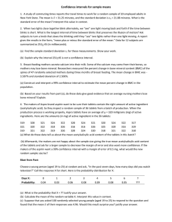
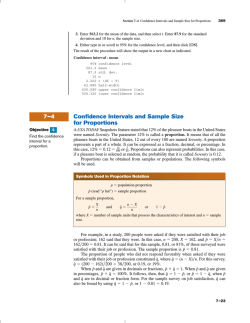
Chapter 7: Estimates and Sample Sizes 7.1 Overview Inferential statistics involve using sample data toвЂ¦ 1. 2. 7.2 Estimating a Population Proportion Notation for Proportions: p= pЛ† пЂЅ x = n qЛ† пЂЅ 1 пЂ p = пѓ when working with a percentage, express it in ___________ form Point estimate: пѓ if we want to estimate a population proportion with a single value, the best estimate is pЛ† пѓ we use pЛ† as the point estimate because it is unbiased (the distribution of sample proportions tends to center about the value of p) and it is the most consistent of the estimators that could be used (the standard deviation of sample proportions tends to be smaller than the standard deviation of any other unbiased estimators) пѓ Ex #1: The Pew Research Center conducted a survey of 1007 adults and found that 85% of them know what Twitter is. Based on that result, find the best point estimate of the proportion of all adults who know what Twitter is. 1 пѓ Ex #2: Touch therapists participated in 280 trials of their ability to sense a human energy field. In each trial, a touch therapist was asked to identify which hand was just below the hand of Emily Rosa. Among the 280 trials, there were 123 correct identifications. The success rate pЛ† = 123/280 = 0.44. Using these test results, find the best point estimate of the proportion of all correct selections that would be made if all touch therapists were tested. пѓ Problem with point estimates: it has a serious flaw of not revealing anything about how close our estimate is to the actual population proportion so statisticians have developed confidence intervals to give us a much better sense of how good an estimate is. Confidence Interval (or Interval Estimate): пѓ sometimes abbreviated _____ пѓ associated with a confidence level (such as 0.95 or 95%) that gives us the success rate of the procedure used to construct the confidence interval and is expressed as the probability or area 1 - пЃЎ (lower case Greek alpha) where пЃЎ is the complement of the confidence level Confidence Level: пѓ Also called the degree of confidence or the confidence coefficient пѓ Most common choices for the confidence level are 90% (with пЃЎ = 0.10), 95% (with пЃЎ = 0.05) and 99% (with пЃЎ = 0.01) пѓ 95% is the most common because it provides a good balance between precision (width of the confidence interval) and reliability (expressed by the confidence level) 2 пѓ Ex #1: Based on the sample data of 1007 adults polled where 85% knew what Twitter was, the 0.95 (or 95%) confidence interval estimate of the population proportion is 0.828 < p < 0.872 --Correct interpretation: --Correct interpretation: --Incorrect interpretation: --Incorrect interpretation: пѓ Ex: Based on the sample data of 280 trials of touch therapists, with 44% of trials resulting in correct identification of the hand that was selected: The 0.95 (or 95%) confidence interval estimate of the population proportion p is 0.381 < p < 0.497 --Correct interpretation: --An incorrect interpretation: вЂњThere is a 95% chance that the true value of p will fall between 0.381 and 0.497.вЂќ пѓ p is fixed so the confidence interval limits either contain p or do not --Ex: If a baby has just been born and the doctor is about to announce its gender, itвЂ™s incorrect to say that there is a probability of 0.5 that the baby is a girl. The baby is either a girl or is notвЂ”there is no probability involved. The value of p is fixed so the confidence interval limits either contain p or do not, which is why itвЂ™s incorrect to say that there is a 95% chance that p will fall between values such as 0.828 and 0.872. 3 пѓ Confidence levels tell us the process we are using will, in the long run, result in confidence interval limits that contain the true population proportion 95% of the time (with 95% confidence, we expect that 19 out of 20 samples should result in confidence intervals that do contain the true value of p and 1 out of 20 confidence interval does not contain p) пѓ Ex #1: If p = 0.5 and the 0.95 (or 95%) confidence interval estimate of the population proportion p is 0.381 < p < 0.497. Does this confidence interval contain the population proportion? пѓ Ex #2: Suppose that the proportion of p = 0.90 is the true population proportion of all adults that know what Twitter is. The confidence interval obtained by the Pew Research Center poll is 0.828 < p < 0.872. Does this confidence interval contain the population proportion? The following figure illustrates that with a 95% confidence level, we expect that about 19 out of 20 confidence intervals (or 95%) to contain the true value of p: Note: Some examples in this chapter require that we address some claim made about the population, but in this chapter we do not yet use a formal method of hypothesis testing, so we simply generate a confidence interval & make an informal judgment based on the result. (Results may or may not be consistent with formal hypothesis testing in chapter 8) 4 Critical Values: пѓ Critical values are based on the following observations: 1. Under certain conditions, the sampling distribution of sample proportions can be approximated by a normal distribution. 2. Sample proportions have a relatively small chance (probability = пЃЎ ) of falling in one of the shaded tails in the following figure. 3. Denoting the area of each shaded tail by пЃЎ /2, there is a total probability of пЃЎ that a sample proportion will fall in either of the shaded tails. 4. By the rule of complements, there is a probability of 1 - пЃЎ that a sample proportion will fall between the two shaded regions. 5. The z score separating the right-tail region is commonly denoted by zпЃЎ / 2 and is a critical value because it is on the borderline separating sample proportions that are likely to occur from those that are unlikely. пѓ A critical value zпЃЎ / 2 is the positive z value that is at the vertical boundary separating an area of пЃЎ /2 in the right tail of the standard normal distribution. пѓ The value пЂ zпЃЎ / 2 is at the vertical boundary for the area of пЃЎ /2 in the left tail. пѓ Ex: Find the critical value zпЃЎ / 2 corresponding to a 95% confidence level. 5 пѓ Find the values of пЃЎ Confidence Level and zпЃЎ / 2 for the most common confidence levels пЃЎ Critical Value zпЃЎ / 2 90% 95% 99% Margin of Error: пѓ denoted by ___ пѓ also called the maximum error of the estimate пѓ found by multiplying the critical value and the standard deviation of the sample proportions: E пЂЅ zпЃЎ / 2 п‚· pЛ† qЛ† n Confidence Interval (or Interval Estimate) for the Population Proportion p ( pЛ† - E) < p < ( pЛ† + E) where пѓ Equivalent forms: ( pЛ† - E, pЛ† - E) E пЂЅ zпЃЎ / 2 п‚· or pЛ† qЛ† n ( pЛ† п‚± E) пѓ Confidence interval limits for p should be rounded to 3 significant digits. 6 пѓ Procedure for Constructing a Confidence Interval for p: 1. Verify the requirements are satisfied: --simple random sample --conditions for a binomial distribution are satisfied (fixed # of trials, trials are independent, 2 categories of outcomes, probabilities remain constant for each trial) --there are at least 5 successes & 5 failures) 2. Use Table A-2 to find the critical value zпЃЎ / 2 that corresponds to the desired confidence level 3. Evaluate the margin of error E пЂЅ zпЃЎ / 2 п‚· pЛ† qЛ† n 4. Substitute the values in the general format of the confidence interval: ( pЛ† - E) < p < ( pЛ† + E) 5. Round the resulting confidence interval limits to 3 significant digits пѓ Ex: Touch therapists participated in 280 trials of their ability to sense a human energy field. In each trial, a touch therapist was asked to identify which hand was just below the hand of Emily Rosa. Among the 280 trials, there were 123 correct identifications. The sample results are n = 280 and pЛ† = 123/280 = 0.439286 --Find the margin of error that corresponds to a 95% confidence level: --Find the 95% confidence interval estimate of the population proportion p 7 --How would you express the confidence interval and margin of error? пѓ Ex: A Pew Research Center poll of 1007 randomly selected U.S. adults showed that 85% of the respondents know what Twitter is. The sample results are n = 1007 and pЛ† = 0.85. a. Find the margin of error E that corresponds to a 90% confidence level. b. Find the 95% confidence interval estimate of the population proportion p. c. Based on the results, can we safely conclude that more than 75% of adults know what Twitter is? 8 Sample Size for Estimating Proportion p: [ zпЃЎ / 2 ]2 pЛ† qЛ† пѓ When an estimate pЛ† is known: n пЂЅ E2 пѓ When no estimate pЛ† is known: n пЂЅ [ zпЃЎ / 2 ]2 (0.25) E2 пѓ If the computed sample size is not a whole number, ROUND IT UP to the next higher number. пѓ Ex: The ways that we communicate have been dramatically affected by the use of answering machines, fax machines, voice mail, and email. Suppose a sociologist wants to determine the current percentage of U.S. households using email. How many households must be surveyed in order to be 95% confident that the sample percentage is in error by no more than four percentage points? a. Use this result from an earlier study: In 1997, 16.9% of U.S. households used email (based on data from the World Almanac & Book of Facts) b. Assume that we have no prior information suggesting a possible value of pЛ† . --By comparing these results, we can see that if we have no prior knowledge, a larger sample is required to achieve the same results as when the value of pЛ† can be estimated. 9 пѓ Common Errors: 1. DonвЂ™t make the mistake of using E = 4 as the margin of error for вЂњ4 percentage points.вЂќ Instead E should be 0.04. 2. Be sure to substitute the critical z score for zпЃЎ / 2 пѓ Note that the population size is irrelevant, and the sample size does not need to be some percentage of the population. пѓ Ex: Gap, Banana Republic, J.Crew, Yahoo, and America Online are just a few of the many companies interested in knowing the percentage of adults who buy clothing online. How many adults must be surveyed in order to be 99% confident that the sample percentage is in error by no more than 3 percentage points? --Use this recent result from the Census Bureau: 66% of adults buy clothing online and assume that we have no prior information suggesting a possible value of the proportion. Finding the Point Estimate and E from a Confidence Interval: пѓ If we know the confidence interval limits we can find the sample proportion or best point estimate ( pЛ† ) and the margin of error (E) пѓ It may help us better understand a confidence interval that might have been obtained from a journal or technology. --Point Estimate of p: pЛ† = --Margin of Error: E= 10 пѓ Ex: The article вЂњHigh-dose nicotine patch therapyвЂќ includes the following statement: вЂњOf the 71 subjects, 70% were abstinent from smoking at 8 weeks (95% confidence interval [CI], 58% to 81%).вЂќ Use this statement to find the point estimate and the margin of error. 11 7.3 Estimating a Population Mean 3 Main Concepts about Estimating a Population Mean: 1. Point estimate: The sample mean x is the best point estimate (or single value estimate) of the population mean Вµ. 2. Confidence Interval: We can use a sample mean to construct a confidence interval estimate of the true value of a population mean, and we should know how to construct & interpret such confidence intervals. 3. Sample Size: We should know how to find the sample size necessary to estimate a population mean. The sample mean x is the best point estimate of the population mean Вµ becauseвЂ¦ --For all populations, the sample mean is an unbiased estimator of the population mean --For many populations, the distribution of the sample means x tends to be more consistent than the distributions of other sample statistics --Ex #1: Data set 1 in Appendix B includes pulse rates (in beats per minute) of randomly selected women, and here are the statistics: n = 40, x = 76.3 and s = 12.5. Use this sample to find the best point estimate of the population mean of pulse rates for all women. Estimating a Population Mean: пѓ ItвЂ™s rare that we want to estimate the unknown population mean but somehow know what the value of the population standard deviation Пѓ. The realistic situation is that Пѓ is unknown. пѓ When Пѓ is unknown, we use the ____________________________ пѓ When Пѓ is known, we use the ____________________________ 12 Part I: Estimating a Population Mean when Пѓ is unknown Requirements: 1. The sample is a simple random sample 2. The value of the population standard deviation Пѓ is unknown 3. The population approximated a normal distribution and/or n > 30 Confidence Intervals: t distribution: If a population has a normal distribution, then the following distribution is a t distribution for all samples of size n: t пЂЅ xпЂпЃ s n пѓ Critical values denoted by tпЃЎ / 2 can be found by locating the appropriate number of degrees of freedom in the left column of table A-3 and finding the corresponding area across the top of the table. Degrees of Freedom: Degrees of freedom = sample size minus 1 = пѓ Ex #1: If students have quiz scores with a mean of 80, we can freely assign values to the 1st 9 scores, but the 10th score must be determined. The sum of the 10 scores must be 800, so the 10 th score must equal 800 minus the sum of the first 9 scores. пѓ Ex #2: A sample size of n = 23 is a simple random sample selected from a normally distributed population. Find the critical value tпЃЎ / 2 corresponding to a 95% confidence level. пѓ Ex #3: A sample size of n = 12 is a simple random sample selected from a normally distributed population. Find the critical value tпЃЎ / 2 corresponding to a 99% confidence level. 13 Margin of Error E for the Estimate of пЃ (with Пѓ unknown): E пЂЅ tпЃЎ / 2 п‚· s n where has n вЂ“ 1 degrees of freedom tпЃЎ / 2 Confidence Interval for the Estimate of пЃ (with Пѓ unknown): ( x - E) < пЃ < ( x + E) where E пЂЅ tпЃЎ / 2 п‚· s n пѓ Procedure for Constructing a Confidence Interval for пЃ (with Пѓ unknown): 1. Verify the requirements are satisfied (simple random sample, either the population is normally distributed or n > 30) 2. Using n вЂ“ 1 degrees of freedom and table A-3, find the critical value tпЃЎ / 2 that corresponds to the desired confidence level (вЂњarea in 2 tailsвЂќ) 3. Evaluate the margin of error E пЂЅ tпЃЎ / 2 п‚· s n 4. Substitute the values into the general format for the confidence interval: ( x - E) < пЃ < ( x + E) 5. If the original set of data is used, round to one more decimal place than is used in the original data set. If using summary statistics, round the confidence interval limits to the same number of decimal places used for the sample mean. пѓ Interpreting a Confidence Interval for for пЃ : Correct interpretations: вЂњWe are 95% confident that the interval from 58.1 to 63.3 actually does contain the true value of the population mean Вµ.вЂќ OR вЂњIf we were to select many different samples of the same size and construct the corresponding confidence intervals, in the long run 95% of them would actually contain the value of the population mean Вµ.вЂќ Incorrect interpretations: вЂњThere is a 95% chance that the population mean Вµ will fall between 58.1 and 63.3.вЂќ OR вЂњ95% of sample means fall between 58.1 and 63.3.вЂќ 14 *Note: In this chapter, we will use a confidence interval to address a claim about a population mean Вµ and make an informal judgment. In chapter 8, we will look at additional adjustments that must be made in order to formally test the hypothesis. --Ex #1: Listed in the accompanying stemplot are the ages of applicants who were unsuccessful in winning promotion. There is an important larger issue of whether these applicants suffered age discrimination, but for now weвЂ™ll focus on the simple issue of using those values as a sample for the purpose of estimating the mean of a larger population. Assume that the sample is a simple random sample and use the sample data with a 95% confidence level to find both the margin of error E and the confidence interval for пЃ . Stemplot of Ages 3 4778 4 12344555689 5 3344567 6 0 15 --Ex #2: Listed below are speeds (mi/h) measured from southbound traffic on I-280 near Cupertino, California. This simple random sample was obtained at 3:30 pm on a weekday. The speed limit for this road is 65 mi/h. Use the sample data to construct a 99% confidence interval for the mean speed. What does the confidence interval suggest about the speed limit? 62 61 61 57 61 54 59 58 59 69 60 67 16 пѓ Important Properties of the t Distribution: 1. The t distribution is different for different sample sizes 2. The t distribution has the same general symmetric bell shape as the standard normal distribution but it reflects greater variability (with wider distributions) that is expected with small samples. 3. The t distribution has a mean of t = 0. 4. The standard deviation of the t distribution varies with the sample size, but is greater than 1 (unlike standard normal distribution) 5. As the sample size n gets larger, the t distribution gets closer to the standard normal distribution. Choosing the Appropriate Distribution: Note: The nonparametric methods are described in chapter 13 and are not covered in this course. 17 Or use the following table (which is included on your reference sheets): Inferences about Вµ: choosing between t and normal distributions t distribution Normal distribution Nonparametric method or bootstrapping Пѓ is not known and normally distributed population OR Пѓ is not known and n > 30 Пѓ is known and normally distributed population OR Пѓ is known and n > 30 Population is not normally distributed and n < 30 пѓ Ex #1: Assuming that you plan to construct a confidence interval for the population mean пЃ , use the given data to determine whether the margin of error E should be calculated using a critical value of distribution), a critical value of zпЃЎ / 2 (from the normal tпЃЎ / 2 (from a t distribution), or neither (so the methods from this course cannot be used). a. n = 150, x = 100, and s = 15, and the population has a skewed distribution b. n = 8, x = 100, and s = 15, and the population has a normal distribution c. n = 8, x = 100, and s = 15, and the population has a very skewed distribution d. n = 150, x = 100, and Пѓ = 15, and the distribution is skewed e. n = 8, x = 100, and Пѓ = 15, and the distribution is extremely skewed 18 Part II: Estimating a Population Mean when Пѓ is known Requirements: 1. The sample is a simple random sample 2. The value of the population standard deviation Пѓ is known 3. The population approximated a normal distribution and/or n > 30 Margin of Error E for the Estimate of пЃ (with Пѓ known): E пЂЅ zпЃЎ / 2 п‚· пЃі n Confidence Interval Estimate of the Population Mean пЃ (with Пѓ known): ( x - E) < p < ( x + E) пѓ Equivalent forms: where ( x - E, x - E) E пЂЅ zпЃЎ / 2 п‚· пЃі n ( x п‚± E) or пѓ Procedure for Constructing a Confidence Interval for пЃ (with Пѓ known): 1. Verify that the requirements are satisfied (simple random sample, Пѓ is known, either the population approximates a normal distribution and/or n > 30) 2. Use table A-2 to find the critical value zпЃЎ / 2 that corresponds to the desired confidence level. (Note: There is no need to find the degrees of freedom because we are using the standard normal distribution) 3. Evaluate the margin of error: E пЂЅ zпЃЎ / 2 п‚· пЃі n 4. Substitute the values into the general format for the confidence interval: ( x - E) < Вµ < ( x + E) 5. Round the resulting values according to the following rules: -When using the original set of data to construct a confidence interval, round to one more decimal that the original set of data 19 -When the original set of data is unknown, round the confidence interval limits to the same number of decimal places used for the sample mean 6. Interpret the confidence interval correctly: вЂњWe are 95% confident that the interval from 72.4 to 80.2 actually does contain the true value of пЃ вЂќ -Because пЃ is a fixed constant, it would be wrong to say that вЂњ95% of all data values are between 72.4 and 80.2вЂќ --Ex #1: For the sample of pulse rates of women in data set 1 in Appendix B, we have n = 40 and x = 76.3, and the sample is a simple random sample. Assume that Пѓ is known to be 12.5. Using a 95% confidence level, find the margin of error E and the confidence interval for пЃ . 20 --Ex #2: Listed below are speeds (mi/h) measured from southbound traffic on I-280 near Cupertino, California where the speed limit is 65 mi/h. This simple random sample was obtained at 3:30 pm on a weekday and the sample mean x was found to be 60.67 mi/h. Construct a 99% confidence interval estimate of the population mean by assuming that Пѓ is known to be 4.1. 62 61 61 57 61 54 59 58 59 69 60 67 Generating confidence intervals using the TI-83/84 plus calculator: Find the values for standard deviation (s or Пѓ), the sample mean ( x ), the sample size (n), and the confidence levelвЂ”either given in the question or using 1-variable stats Then press STATвЂ”go over to TESTSвЂ”and choose eitherвЂ¦ TInterval if Пѓ is unknown OR ZInterval if Пѓ is known. 21 Finding a Point Estimate and Margin of Error from a Confidence Interval: пѓ Point Estimate of пЃ : x = пѓ Margin of Error: E= пѓ Ex: In analyzing the ages of all Queen Mary stowaways, we are 95% confident that the limits of 24.065 and 27.218 contain the value of the mean age of the stowaways. Use the given confidence interval to find the point estimate x and the margin of error E. Treat the values as sample data randomly selected from a large population. пѓ Ex #2: The following data describes the results from counts of chocolate chips in a sample of 32 Chips Ahoy chewy cookies. It shows the confidence interval limits for a 95% confidence level. Find the values of the best point estimate x and the margin of error E. n = 32 x = 19.094 s = 2.68 18.128 < Вµ < 20.06 22 Finding the Sample Size for Estimating the Population Mean пЃ : пѓ© zпЃЎ / 2пЃі пѓ№ Use the formula: n пЂЅ пѓЄ пѓє пѓ« E пѓ» Where zпЃЎ / 2 2 = E= Пѓ= --If the result is not a whole number, always increase the value of n to the next larger whole number --To use the formula to find the sample size, you must know the population standard deviation Пѓ --What if you donвЂ™t know Пѓ? (Just to find sample sizeвЂ”not to construct a confidence interval) 1. Use the range rule of thumb to estimate the standard deviation Пѓ в‰€ range / 4 2. Start the sample collection process & using the first several values, calculate the sample standard deviation s and use it in place of Пѓ. 3. Estimate the value of Пѓ by using the results of some other study that was done earlier. -Note: Using a value for Пѓ that is larger than the true value would make the sample size larger than necessary, but using a value for Пѓ that is too small would result in a sample size that is inadequate. *Sample size determination cannot be found using the TI-83/84 graphing calculator. 23 --Ex #1: Assume that we want to estimate the mean IQ score for the population of statistics professors. How many statistics professors must be randomly selected for IQ tests if we want 95% confidence that the sample mean is within 2 IQ points of the population mean? --Ex #2: Assume that the want to estimate the mean IQ score for the population of statistics students. How many statistics students must be randomly selected for IQ tests if we want 99% confidence that the sample mean is within 3 IQ points of the population mean? 24 7.4 Estimating a Population Variance Requirements for Estimating a Population Variance or Standard Deviation: 1. The sample is a simple random sample 2. The population must have normally distributed values (even if the sample is large) Chi-Square Distribution: пЃЈ пЂЅ 2 (n пЂ 1) s 2 пЃі2 where n = sВІ = ПѓВІ = пѓ pronounced вЂњkigh squareвЂќ пѓ use table A-4 to find critical values which correspond to an area given in the top row of the table and that area represents the ______________ _____________________________ of the critical value. Note: Use the closest number of degrees of freedom unless it is exactly midway between two values (then find the mean of the two пЃЈ 2 values) пѓ Properties of the Chi-Square Distribution: 1. The chi-square distribution is not symmetric. As the number of degrees of freedom increases, the distribution becomes more symmetric. 2. The values of chi-square can be zero or positive, but cannot be negative. 3. The chi-square distribution is different for each number of degrees of freedom and the number of degrees of freedom is given by df = n вЂ“ 1 (in this section). *Because the chi-square distribution is not symmetric, a confidence interval for Пѓ2 does not fit a format of s2 вЂ“ E < Пѓ2 < s2 + E, so we must do separate calculations for the upper and lower confidence interval limits. 25 пѓ Ex #1: Find the critical values of пЃЈ 2 that determine critical regions containing an area of 0.025 in each tail. Assume that the relevant sample size is 10 so that the number of degrees of freedom is 10 вЂ“ 1 = 9. пѓ Ex #2: A simple random sample of 22 IQ scores is obtained. The 22 full IQ scores for the group with medium exposure to lead have a standard deviation of 14.3. Consider the sample to be a simple random sample and use a 2 99% confidence level to find the critical values of of пЃЈ used to estimate of the population standard deviation Пѓ. 26 пѓ Estimators of ПѓВІ: --The sample variance sВІis the best point estimate of the population variance ПѓВІ (because sample variances sВІ tend to target the value of the population variance ПѓВІ) --The sample standard deviation s is commonly used as a point estimate of Пѓ (even though it is a biased estimate) Constructing a confidence interval for the population variance Пѓ2 where пЃЈ L2 = the left-tailed critical value (n пЂ 1) s 2 пЃЈ 2 R < ПѓВІ < (n пЂ 1) s 2 пЃЈ and пЃЈ R2 = the right-tailed critical value 2 L пѓ Confidence interval for the population standard deviation Пѓ: (n пЂ 1) s 2 пЃЈ R2 <Пѓ< (n пЂ 1) s 2 пЃЈ L2 пѓ Procedure for Constructing a Confidence Interval for the Population Variance or Standard deviation ПѓВІ or Пѓ: 1. Verify the requirements are satisfied (simple random sample, very close to a normal distribution) 2. Using n вЂ“ 1 degrees of freedom, use table A-4 to find the critical values пЃЈ L2 and пЃЈ R2 that correspond to the desired confidence level. 3. Evaluate the upper and lower limits of the confidence level: (n пЂ 1) s 2 пЃЈ R2 < ПѓВІ < (n пЂ 1) s 2 пЃЈ L2 4. If a confidence interval estimate of Пѓ is desired, take the square root of the upper and lower confidence interval limits and change ПѓВІ to Пѓ. 5. Round to one more decimal place than is used for the original set of data. If using the sample standard deviation or variance, round the confidence interval limits to the same number of decimal places. *Note: The TI-83/84 graphing calculator does not provide confidence intervals for Пѓ or Пѓ2. 27 пѓ Ex #1: Pennies are currently being minted with a standard deviation of 0.0165 g. New equipment is being tested in an attempt to improve quality by reducing variation. A simple random sample of 10 pennies is obtained from pennies manufactured with the new equipment. A normal quantile plot and histogram show that the weights are from a normally distributed population, and the sample has a standard deviation of 0.0125 g. Use the sample results to construct a 95% confidence interval estimate of Пѓ, the standard deviation of the weights of pennies made with the new equipment. Based on the results, does the new equipment appear to be effective in reducing the variation of the weights? пѓ Ex #2: A simple random sample of 22 IQ scores is obtained. The 22 full IQ scores for the group with medium exposure to lead have a standard deviation of 14.3. Consider the sample to be a simple random sample and construct a 99% confidence interval estimate of the population standard deviation Пѓ. 28 Determining Sample Size Necessary for Estimating ПѓВІ: пѓ Procedures are much more complex than determining sample sizes for means and proportions, so we will use the following table: пѓ Ex: We want to estimate Пѓ, the standard deviation of all body temperatures. We want to be 95% confident that our estimate is within 10% of the true value of Пѓ. How large should the sample be? Assume the population is normally distributed. пѓ Ex #2: We want to estimate the population standard deviation Пѓ of all IQ scores of people with exposure to lead. We want to be 99% confident that our estimate is within 5% of the true value of Пѓ. How large should the sample be? Assume that the population is normally distributed. 29