Fast GC/GCMS
Application Book
Chromatography Volume 2
Prof. Luigi Mondello, University of Messina, Italy
Dr. Hans-Ulrich Baier, Shimadzu Deutschland GmbH, Germany
Fast GC and GC/MS using narrow-bore columns:
Principles and Applications
Fast GC/GCMS
Application Book
Windows is a Trademark of Microsoft
Corporation.
© Copyright:
Shimadzu Deutschland GmbH, Duisburg.
Reprint, in whole or in part, is subject to the
permission of the editorial office.
Design and Production:
ME Werbeagentur GWA · Düsseldorf
Editorial Team:
Prof. Luigi Mondello, University of Messina, Italy
Dr. Hans-Ulrich Baier, Shimadzu Deutschland GmbH,
Germany
Publisher:
Shimadzu Deutschland GmbH
Albert-Hahn-Str. 6 -10 · 47269 Duisburg, Germany
Telephone: + 49 (0) 203 7687-0
+ 49 (0) 203 766625
Telefax:
Email:
[email protected]
Internet: www.shimadzu.de
Application Book Chromatography Volume 2
Fast GC/GCMS
15
19
23
31
32
37
39
III. Injection requirements in fast GC
IV. Detector requirements in fast GC
1. Conventional detectors
2. Mass spectrometric detector (quadrupole MS)
V. Applications in food analysis
1. Organophosphorous pesticides in food matrices
(GC-FPD, GC-FTD, GC/MS)
2. The analysis of organochlorine pesticides in food matrices
using GC-ECD and NCI GC/MS.
3. Analysis of butter fatty acid methyl esters (GC-FID)
VI. Application in the petrochemical field
Kerosene analysis (GC-FID)
VII. Applications in the fields of flavors & fragrances
1. Potential allergens in perfumes
2. Quality control of flavors (GC-FID)
VIII. Application in the environmental field
PCB analysis with GC-ECD detection
IX. Summary
7
11
Overview
II. Basics of separation in fast GC
1. Column and stationary phase
2. Length and peak resolution
3. Inner diameter and peak resolution
4. Film thickness and peak resolution
5. Type of carrier gas and average linear velocity
6. GC hardware requirements
I.
Content
8
G
I. OVERVIEW
Nowadays in daily routine work,
apart from increased analytical
sensitivity, demands are also
made on the efficiency in terms
of speed of the laboratory equipment. Regarding the rapidity of
analysis, two aspects need to be
considered:
The capillary columns used may
have solid fillings (PLOT
columns) or a liquid film as a
stationary phase. The latter are
employed in gas liquid chromatography (GLC), which is the
subject of the present booklet.
In GLC, analyte separation is
achieved by means of a dynamic
thermal equilibrium between the
stationary phase (liquid) and
mobile phase (gas). The dimensions of the columns employed,
which vary depending on the
application, generally range from
inner diameters between 0.25 to
0.53 mm and lengths from 25 to
60 m. The film thickness selected, dependent on the boiling
points of the analytes, usually
ranges from 0.25 to 1 µm (in
some cases up to 3 µm or even
more).
as chromatography is a wellestablished technique, employed
in many applicational fields such
as environmental, food, petrochemical and pharmaceutical
analysis [1].
An example of the validity of
this approach is illustrated in
Figure I.1 (lower chromatogram)
The present overview is focussed
on the use of narrow-bore
columns in fast gas chromatography. As mentioned, this type of
approach enables substantial
reductions in GC run-times
without compromising the chromatographic resolution.
These analytical tools enable a
considerable reduction of analyses times while peak resolution is
essentially maintained. Another
approach worthy of mention is
the use of multicapillary columns
[6 - 8] with more than 900 capillary tubes with inner diameters
of about 40 µm.
It is well known that analytical
time costs may be very high in
standard GC applications. In the
last few years, fast GC methods
have been shown to be suitable
for routine laboratory work. In
this respect, the employment of
narrow-bore columns is of particular interest [2 - 5].
2. The efficiency of the analytical
equipment employed
1. The costs in terms of time
required, for example in quality
control analysis
All the chromatograms shown
were recorded with a Shimadzu
GC-2010 or GCMS-QP2010
with an AOC-20i autoinjector
and GCsolution or GCMSsolution software for data elaboration.
However, the GC hardware has
to meet some requirements in
order to enable the efficient use
of narrow-bore columns. In the
following chapters, general and
fundamental issues relative to
fast gas chromatography are discussed (injection systems, capillary columns, carrier gas and
detector characteristics).
which reports a fast GC analysis
(RTX-5 10 m, 0.1 mm ID, 0.4 µm
film thickness) on a capillary column test mixture (Grob test mixture, Macherey und Nagel). The
conditions were as follows: injection mode: split (200 : 1), average
linear carrier gas velocity: 120
cm/s (502 kPa, H2), temperature
program: from 140 °C at 60
°C/min to 280 °C. A conventional application (DB 5 30 m, 0.25
mm ID, 0.25 µm film thickness)
on the same matrix is also shown
in the diagram (upper chromatogram). As apparent, the
degree of separation is even better in the fast GC application
while a speed gain of approximately 8 times is attained.
Chromatography Volume 2
0
2
4
6
x 104
1
3
5
x 106
0.25
1
6.0
2
1
3
4
0.50
7.0
Chromatography Volume 2
2
5
3
8.0
4
0.75
9.0
5
Minutes
1.00
6
Minutes
10.0
11.0
6
1.25
12.0
7
7
8
8
1.50
13.0
14.0
9
9
1.75
FWHM = 0.48 s
15.0
FWHM = 3 s
Peak identification:
1) n-Decane
2) n-Octanole
3) n-Undecane
4) 2.6-Dimethylphenole
5) 2.6-Dimethylaniline
6) Decane acid methyl ester
7) Undecane acid methyl ester
8) Dicyclohexylamine
9) Dodecane acid methyl ester
Top: Chromatogram recorded with a
Grob test mixture using a DB5 30 m,
0.25 mm, 0.25 µm column.
Bottom: Chromatogram recorded
with the Grob test mixture using a
RTX-5 10 m, 0.1 mm, 0.4 µm column.
Figure I.1:
I. OVERVIEW
9
12
An important issue in fast GC
regards the narrow-bore column
Both the polarity and the boiling
points of the sample analytes
must be considered during the
selection of a specific stationary
phase material. Nowadays, several phase materials are available
for typical fast GC applications.
Apart from the choice of the stationary phase, other important
column parameters to be optimized are length, internal diameter
and film thickness.
sample capacity, which is considerably lower than with conventional capillaries (this aspect will
be discussed later).
1. Column and stationary phase
II. BASICS OF SEPARATION IN FAST GC
2
Dt
R ≈ EL
Wb
• Column length for fast GC:
10 - 15 m
Consequently, doubling the column length achieves a gain of
resolution of a factor of only
1.41. Therefore typical column
lengths in fast GC are within the
10 - 15 m range.
5
thus the resolution is proportional to the square root of the
column length:
4
L
N = ––––––– L = column length
HETP
where tM is the time required for
an unretained analyte to pass
through the column (generally
referred to as dead time). The
relationship between the length
of the column, N and height of a
theoretical plate (HETP) is as
follows:
Figure II.1: Peak resolution parameters for two subsequent peaks in a
chromatogram
Wa
t’R
k’2
t’R 2
k’= ––––
, a = ––––
= ––––
tM
k’1
t’R 1
with k´2 = capacity factor of the
more retained solute and
a = separation factor:
3
k’2
EN a
R = –––– –––– ––––
4 a – 1 k’2 + 1
Resolution (R) on the other hand
depends on the capacity factor k
and the plate number N in the
following equation [9]:
2
it
R = ––––––––––––
1_ [w + w ]
b
2 a
where wb is the base peak width
and tR is the retention time. Peak
resolution is of particular interest
as the main aim is to reduce the
analysis time while maintaining
the column resolving power (Figure II.2). The resolution between
two peaks is defined as:
1
tR
N = 16 • ––––
wb
The number of theoretical plates N of a column is a measure of
its separation efficiency and is
defined as [9]:
2. Length and peak resolution
Chromatography Volume 2
KD = k’ • b
With regard to the experimental
curves, the HETP values are
derived from the peak widths
(eq. 1 and 4) and are plotted as a
function of the average linear
velocity of the carrier gas.
A typical curve is shown in Fig-
For further elucidation, the so
called van Deemter curves [9]
will be discussed in the following
chapter where HETP values for
different capillary columns are
plotted versus the average linear
carrier gas velocity [u].
0.25 µm, the phase ratio is equal
to approximately 250. This is a
typical phase ratio value for a
medium boiling point analyte
range. In general, this parameter
is used by the analyst to make a
first selection of the column
dimension for a given distribution of analyte boiling points.
Column manufacturers usually
offer schematic tables in their
catalogues giving an overview of
typical b values for different
applications. The value for b typically varies between 50 (columns
with thick films for volatiles) and
530 (wide-bore columns, high
boilers).
On the other hand, it should also
be suited to the boiling points of
the analytes (see also b). Since
the column sample capacity also
decreases with the film thickness
(less amount of stationary phase),
the split ratio needs to be adjusted depending on the concentration of the sample. High split
ratios ensure that the sample is
The linear relationship between
peak resolution and stationary
phase thickness requires the latter to be as thin as possible in
fast GC.
• Columns in fast GC:
film thicknesses are typically
0.1 µm (≤ 0.4 mm)
As a conclusion, a typical film
thickness in fast GC of 0.1 µm
(dI = 0.1 mm, b = 250) is used.
In specific cases of highly volatile compounds film thicknesses
of up to 0.4 µm (b = 62.5 for
0.1 mm dI) may be used.
transferred rapidly from the
glass insert to the column (see
III. Injection).
1.0
0.9
0.8
0.7
0.6
0.5
0.4
0.3
0.2
0.1
0.0
0
100
150
Average Linear Velocity (cm/sec)
50
200
10 m x 0.10 mm i.d. 0.10 µm film
30 m x 0.25 mm i.d. 0.25 µm film
isothermal (150 °C)
Van Deemter Curves C16 : 0 FAME
Conventional and Ultra Fast
II. BASICS OF SEPARATION IN FAST GC
7
HETPmin prop dI
ure II.2 for 2 columns of differing inner diameter [10]. The plate
height is characterized by a minimum value (HETPmin) at the
optimum linear velocity [9].
Both columns have a b value of
approximately 250. For columns
with such a high phase ratio value, the resistance to mass transfer
in the stationary phase can be
neglected and HETPmin can
therefore be approximated to the
column ID [10]:
• Columns for fast GC:
inner diameter ≤ 0.15 mm
13
As seen from equation 7 and Figure II.2 the minimum theoretical
plate height decreases linearly
with the capillary column inner
diameter. Furthermore, the
ascending part of the curves rises
more gradually, enabling the
application of higher than optimum velocities with little loss in
terms of resolving power. To
conclude, the inner diameter of
suitable columns for fast GC are:
Figure II.2: Van Deemter curves [10] for 0.25 mm and 0.1 mm ID columns.
The phase ratio is 250 in both cases.
4. Film thickness and peak resolution
The distribution coefficient KD
is dependent on the temperature
and the physical and chemical
properties of the analytes and
stationary phase. The retention
time is therefore determined by
the inner diameter, film thickness
and length of the column for
fixed material properties. For
typical inner diameters and film
thicknesses such as 0.25 mm and
where:
dI,df = inner diameter/film
thickness of the column
KD = distribution constant
b
= phase ratio
6
dI
b ≈ ––––
4df
In general, the chromatographic
peak width increases with the
retention time due to resistance
to mass transfer in the mobile
and stationary phase contributions. The influence of the inner
diameter with respect to the
theoretical plate number is now
considered. The basic equation
for the retention of a substance
is [9]:
3. Inner diameter and peak resolution
Chromatography Volume 2
HETP (mm)
20
40
In most applications, a linear
temperature program is employed rather than isothermal analysis. Under isobaric conditions,
linear temperature ramps are
higher compared to standard GC
[70 °C/min linear and higher
(ballistic)]
• high separation efficiency 35
14
• temperature program
average linear carrier gas velocity
should be constant over the
entire analysis (the constant linear velocity mode requires a
pressure program)
large head pressure, high maximum operational head pressure
(up to 970 kPa)
autoinjector, rapid injection, high
split ratios (see chapter III.)
35
• reduced internal diameter 35
35
GC instrument requirements
The aforementioned issues have direct consequences on GC instrumentation requirements such as injection system, carrier gas pneumatics, column oven heating/cooling and detection. These aspects are
summarized as follows:
• fast injection
60
[u] cm/s
N2
80
H2
He
high sampling rates and low
filter time constants (250 Hz,
4 ms-conventional detectors)
This is achieved by the application of a pressure program automatically calculated by the GC software, and leads to a final pressure
of 660 kPa at 280 °C. The cooling time for this analysis is below
2 minutes and the cycle time is under 4 minutes.
In the example illustrated in Figure I.1 (see page 9), a 120 cm/s average linear velocity was applied. In order to obtain this velocity an
initial pressure of 502 kPa was required at the initial temperature of
140 °C. The gas chromatograph maintains the average linear velocity
constant over the temperature program (60 °C/min up to 280 °C).
The data in brackets refer to specifications of the GC-2010.
35
high split ratios should be
available (total flow of up to
1200 mL/min)
35
• high concentration range
• sharp peaks in fast GC
fast cooling of the GC oven
(2 min from 280 °C to 100 °C)
35
Consequently, the gas chromatograph should have an automatic
pressure regulator in order to
keep the average linear velocity
constant over the entire temperature program. This issue leads
directly to fast GC hardware
requirements.
with temperature. Hence, the
separation efficiency is reduced
as the temperature increases (the
optimum velocity is generally
selected for the initial temperature) and the analysis time is also
prolonged when compared to
constant velocity conditions.
Chromatography Volume 2
• high final temperature
average linear velocity decreases
with increasing temperatures [9].
This is due to the fact that the
gas viscosity increases linearly
Figure II.3: Van Deemter curves measured using different carrier gases
(Shimadzu Corporation, Kyoto, Japan)
0.4
0.8
HETP (mm)
Capillary column: OV-101 25 m, 0.25 mm ID. 0.4 µm film
HETP – [u] curve for C17 at 175 °C with k = 4.95
6. GC hardware requirements
As can be seen, the minimum
HETP for the hydrogen curve is
attained at a higher average linear
velocity when compared to other
carrier gas types. In addition, the
ascending part of the curve rises
more gradually for the hydrogen
curve. The data illustrated in
Figure II.3 were derived from a
0.25 mm ID column. In the case
of smaller inner diameters, as
already referred to, the ascending
part rises even more gradually as
mentioned in section 3.
In fast GC applications, particular attention must be paid to the
type of carrier gas used. The Van
Deemter curves have different
minima for different gas types
[9]. This factor is shown in detail
in Figure II.3.
5. Type of carrier gas and average linear velocity
II. BASICS OF SEPARATION IN FAST GC
16
Figure III.1: Schematic of a
split/splitless injector (SPL-17):
Fc: carrier gas, Fs: split flow,
Fl: Flow through glass insert
Fl
Column flow
Splitting point
Fs
1.0
1.5
Standard glass insert
Glass insert with small
inner diameter
Minutes
2.0
2.5
3.0
3.5
4.0
Figure III.2 shows the effect
of glass insert dimensions on
peak width. Here the Grob test
mix was analyzed with a stan-
1. Glass insert
1. Use of glass insert with small
inner diameter to enhance
purging with carrier gas.
2. In the case of splitless injection: high pressure injection.
At low concentration ranges (low
split ratio or splitless injection):
Samples with a high concentration: high split ratio
Whenever splitless injection is
applied in fast GC, a reduced
volume glass insert and high
pressure injection are required.
In general, sample transfer has a
profound influence on peak
shape and needs to be optimized:
split/splitless injector results in a
vapor volume of about 175 µL at
280 °C and a head pressure of
100 kPa. In the case of acetone
as solvent the vapor volume
under the same conditions is
about 310 µL. Typical glass insert
volumes on the other hand are
within 1- 2 mL.
Figure III.2: Chromatograms relative to a Grob test mixture.
Top: reduced ID (inner diameter) glass insert = 1 mm.
Bottom: standard glass insert, 4 mm ID.
0.5
The sharpness of the peaks is
also affected. For example, a
1 µL n-hexane injection into a
In the case of a relatively slow
sample transfer rate (such as in
splitless injection, see Figure
III.1), this results in an initial
sample band broadening on the
first part of the column [11],
which has a considerable effect
on the whole separation efficiency. The well-known solvent
effect indicated by Grob [11] is
not applicable as the column initial temperature has to be set
below the solvent boiling point,
making the analysis time longer,
and in addition the film thickness
is very small. This requires that
the glass insert is not overloaded
with vapor after liquid injection
[11].
n-Decane
Glass insert
Dimethylaniline
Split
n-Octanole
n-Undecane
Dimethylphenole
Purge
Decane acid methyl ester
Carrier
As can be observed in Figure I.1
(see page 9), the peak widths at
half height (FWHM) are below
0.5 s, much less if compared to
conventional GC (about 3 s).
The peak width is affected by the
time needed to transfer the sample, vaporized in the glass insert,
onto the column. The sample
transfer must be fast enough
(movement of syringe plunger,
purge speed of the glass insert).
Dicyclohexylamine
Fc
Chromatography Volume 2
Injection requirements in fast GC
Undecane acid methyl ester
III. INJECTION REQUIREMENTS IN FAST GC
Dodecane acid methyl ester
As discussed in chapter II (section 5), the carrier gas average
linear velocity has a great influence on the column separation
efficiency. The applied head pressure is therefore of great importance after sample transfer to the
column. In this respect, it is possible to apply an increased pressure just for sample transfer (typically for 30 s to 1 min). After
this period the pressure is
dropped automatically to the
analytical pressure to ensure peak
resolution. This operation mode
2. High pressure injection
In the chromatogram illustrated
in Figure I.1 (see page 9), a 200 : 1
split ratio was selected. For peak
no 1, the peak width measured
with the standard glass insert was
FWHM = 0.42 s (split ratio
200 : 1) in contrast to 1.56 s in
Figure III.2 – bottom (split ratio
40 : 1).
dard glass insert (4 mm inner
diameter – bottom) and a glass
insert with a 1 mm ID (top). All
other parameters remained
unchanged. In particular, the
peak widths of the less retained
volatile components were narrower when the glass insert
dimension was reduced. The
effect of purging, which was
more effective for the reduced ID
glass insert, is clearly demonstrated. The split ratio was 40 : 1
in both cases. For increased split
ratios the peak widths were also
narrower when using the standard glass insert.
Chromatography Volume 2
The maximum amount of sample
which may be introduced onto a
capillary column without overloading is lower for narrow-bore
columns. When excessive sample
amounts are injected onto a capillary, peak fronting effects are
observed [9]. The generation of
asymmetric peaks may obviously
lead to a substantial loss in resolution. Consequently, the injected sample amount must be below
a threshold value, as may be
observed in Figure III.3 [10].
Here the plate number (calculated from the peak width according to eq. 1) and hence separation
efficiency is plotted as a function
of sample amount for two
columns of different internal
diameter. It can be seen that for
standard columns (0.25 mm ID)
up to 50 ng solute quantities may
be injected with little or no loss
of separation efficiency. For a
narrow-bore column with a 0.1
mm ID, analyte amounts of up to
1 ng may be injected without losing separation efficiency.
3. Sample capacity of capillary
columns
is defined as high pressure injection. Obviously, the purging of
the glass insert is increased when
compared to standard conditions.
In chapter V (section 1), where
analysis of organophosphorous
pesticides is discussed, high pressure injection (600 kPa) was
applied in combination with a
splitless injection technique in
order to optimize peak shapes.
0.1
10.0
Amount injected (ng)
1.0
10 m x 0.10 mm i.d. 0.10 µm film thickness
100.0
1,000.0
25 m x 0.25 mm i.d. 0.25 µm film thickness
17
Figure III.3: Number of theoretical plates as a function of sample amount for two
different columns
60
70
80
90
100
Plate Number X 1000
III. INJECTION REQUIREMENTS IN FAST GC
Filter time t
Time
Signal height = 63.2 %
20
0.030
Mass spectrometric detection is
described in the next section.
As mentioned, typical fast GC
peak widths are 0.5 s or less.
The detection system must meet
a series of requirements in order
to maintain the peak width at
column outlet. In this section the
requirements for FID are discussed, but the principles are
valid for all of the conventional
GC detectors. In general, detector peak broadening may be
caused by two factors. Firstly,
the possible presence of dead
volumes in the sample path.
Modern GC detectors are generally characterized by low dead
volumes. Furthermore, make-up
gas is employed to optimize peak
shapes through an additional
flow (typically 30 mL/min). For
mass flow dependent detectors
In this section, conventional
detectors such as the flame ionization detector (FID), electron
capture detector (ECD), flame
photometric detector (FPD) and
flame thermionic detector (FTD
or NPD) are discussed.
0.031
Filter time constant
0.032
Minutes
0.033
0.034
0.036
100 ms
0.035
50 ms
20 ms
4 ms
200 ms
In modern GC, the detector signal is digitalized in the detector
electronics and the A/D converter passes digital data to the PC.
Due to the presence of RC
chain-containing circuits, any
signal amplifier has a certain
response time with the presence
of some smoothing effect. This
should not influence the peak
width which is determined by
the chromatographic process
prior to the detector (injection
system, column). The parameter
of detector electronics regarding
the response time is usually
referred to as filter time constant
(FTC) [12]. The electronic detector signal amplifier cannot follow
a signal in an infinitely fast way.
It needs a certain time to follow
rapid signal changes. In Figure
IV.1 this parameter is visualized
graphically [12]. A theoretical
step increase of signal is shown
here and the response of detector
amplifiers indicates that it follows the signal with some time
(FID, FPD, FTD) this feature
enhances sensitivity [9].
Chlorodecane was diluted in
methanol. Figure IV.2 shows the
chlorodecane peak which elutes
at 0.0332 min under isothermal
conditions. The filter time constant t was varied from 4 ms to
200 ms. It can be clearly obser-
1. A 0.1 mm ID glass insert and a
0.2 µL injection volume of just
one compound (chlorodecane)
with a high split ratio (600 : 1).
2. Use of a 1 m column with a
0.1 mm ID and 0.1 µm film
thickness; isothermal analysis
at 200 °C.
3. Detector make-up gas flow of
60 mL/min.
This parameter should be
selectable [12] together with the
number of data points recorded
across a peak. In an experiment,
the influence of this parameter
on real peak shapes was measured. The effects of the injection
system and column on band
broadening were reduced as follows:
delay (1-1/et). The time interval
which the detector electronics
needs to reach the (1-1/e) fraction of such a step signal is
defined as filter time constant.
Figure IV.2: FID signal of chlorodecane. The filter time constant t was changed
from 4 to 200 ms. The sampling frequency was 250 Hz in all cases.
0.0
0.5
1.0
1.5
2.0
uV (x 10,000)
1. Conventional detectors
Figure IV.1: Definition of filter time constant t
Signal
Chromatography Volume 2
Filter time constant and sampling frequency
IV. DETECTOR REQUIREMENTS IN FAST GC
2s
Time constant
Figure IV.4: Signal-to-noise ratio as a function of the filter time constant and for different peak widths
(source: GC-2010 operation manual)
04 ms
5 ms
0.2
Half width 0.1 s
Half width 1 s
After peak assignment, the SIM
mode (selected ion monitoring)
out in the full scan mode in
order to perform a MS library
search. In this operation mode,
every data point corresponds to a
complete mass spectrum over the
mass range selected (scan).
0.6
10 ms 20 ms 50 ms 100 ms 200 ms 500 ms 1 s
The most common mass spectrometric detector used in gas chromatography is the quadrupole
MS. With regard to fast GC/MS
analysis, the MS detector obviously needs to be fast enough for
the rapid eluting analyte bands.
For identification purposes,
GC/MS applications are carried
Half width 10 s
0.4
Minutes
Figure IV.3: Chromatograms relative to a kerosene sample recorded at a filter
time constant t of 100 ms and 10 ms respectively
Minutes
0.2 0.4 0.6 0.8 1.0 1.2 1.4 1.6 1.8 2.0 2.2 2.4 2.6 0.2 0.4 0.8 1.0 1.2 1.4 1.6 1.8 2.0 2.2 2.4 2.6
Filter time constant t
21
In order to attain this data, two
parameters of the GC/MS hardware must be considered: firstly,
the mass range selected by the
analyst must cover all the analyte
ion fragments in order to D
may be used in order to increase
the analytical sensitivity.
2. Mass spectrometric detector (quadrupole MS)
A further electronic parameter of
importance is the sampling rate
or, in other words, the number of
data points acquired per second
which are transferred from the
A/D converter to the PC. The
number of points must be sufficient for the proper reconstruction of a Gaussian peak (minimum 10 to 15 data points). If the
number of data points is too low,
data reproducibility is reduced.
The filter time constant and the
sampling frequency parameters
necessary for the range of peak
widths observed in gas chromatography were summarized by
J. V. Hinshaw [12]. The latter
reported that for peak widths
between 0.1 and 0.5 s the filter
time constant and sampling rate
should be about 10 ms and 20 to
100 Hz respectively.
IV. DETECTOR REQUIREMENTS IN FAST GC
0.8
1
1.2
ved that increases in the filter
time constant affects both the
peak retention time and shape as
predicted from theory [12]. The
full width at half maximum for a
t value of 200 ms (a standard
parameter in many GC systems)
is about 3 s, whereas for a t value
of 4 ms the FWHM value is
about 40 ms. The effect of the
filter time constant on peak
shape obviously has a drastic
effect on resolution as shown in
Figure IV.3. The figure illustrates
two kerosene very fast GC chromatograms with applied filter
time constants of 100 and 10 ms
respectively. The improvement in
terms of peak resolution is evident in the 10 ms FTC analysis.
This experiment shows the
importance of detector parameter
optimization in terms of peak
resolution. In addition, the FTC
has a considerable influence on
the signal-to-noise ratio (S/N).
Figure IV.4 shows the normalized signal-to-noise ratio as a
function of the filter time constant. These curves are plotted
for different peak widths. For a
peak width of 0.1 s the optimum
filter time constant is 20 ms with
regard to the S/N ratio. The
optimum FTC value under such
conditions is also dependent on
the sample concentration and
ranges between 4 and 20 ms.
Chromatography Volume 2
Normalized SN ratio
22
Figure IV.6: Linalool peak generated by
a narrow-bore column (FWHM 0.6 s)
and the spectra recorded at the beginning, apex and end of the peak after
background subtraction. Spectra similarities are 94, 96, 94 using the Wiley
MS library.
The true scanning speed of the
quadrupole is calculated by the
scan range divided by the interval
time minus the RF setup time
which ranges from 5 to 10 ms
for the GCMS-QP2010. In Figure IV.6 this is demonstrated by
experimental data. A linalool
peak was scanned with a 20 Hz
scanning frequency and a selected mass range of 30 to 350 amu.
The analysis was carried out with
a SPB5 10 m, 0.1 mm, 0.1 µm column. The peak width at half
height is about 0.6 s and about
1.2 s at the base resulting in
24 data points across the peak.
As can be seen, the quality of the
spectra in three points across the
chromatographic peak is good
(a Wiley library search was performed). The spectra similarities,
94, 96, 94, indicate that there is
no skewing.
perform a library search for component identification (scan). In
this case, the scan speed should
be high enough so that the relative intensities of the fragments
do not change significantly from
point to point across a narrow
peak. In this respect, a low scan
speed would result in low quality
library matches. Secondly, the
sampling frequency, which corresponds to the number of scans
(or the number of SIM data
points) per second, is, as aforementioned, a fundamental parameter. Fast GC/MS applications
require a high quadrupole scan
rate (up to 10,000 amu/s) and, in
addition, a low inter-scan dead
time (reset time of the electronics) so that the sampling rate
may be sufficiently high (up to
50 Hz/100Hz in scan/SIM modes
for the GCMS-QP2010). This
situation is shown in Figure IV.5.
80
120
160
80
120
160
R.Time: 3.922 (Scan#: 3027)
40
m/z
m/z
3.89
R.Time: 3.921 (Scan#: 3026)
40
3.88
200
200
3.90
240
240
3.91
280
280
3.92
Minutes
3.922
20
min.
Linalool
2.4
60
61,307,110
m/z
100
140
Wiley
SI = 97
180
TIC
2.5
20
min.
60
2.4
61,307,110
m/z
100
Scan N +1
3.97
140
Wiley
SI = 98
180
TIC
2.5
20
min.
60
2.4
61,307,110
m/z
100
140
Wiley
SI = 97
RF setup
3.96
Inter-scan time
3.95
1/I = sampling frequency
Scan N
3.94
Intervall I:
m1
m2
3.93
180
TIC
TIC*1.00
2.5
3.98
Chromatography Volume 2
Figure IV.5: Definition of scan speed, inter-scan delay and sampling frequency for a quadrupole MS
100
100
3.87
6,086,271
IV. DETECTOR REQUIREMENTS IN FAST GC
1
2
uV (x 1,000.000)
3
4
5
5
RTX-5: 10 m, 0.1 mm, 0.4 µm
4
6
Trichlorphon
7
8
9
10
11
Minutes
10
Minutes
12
Phosphamidon (Z)
6
Fenthion
15
Tolclophos - Me
Ethion
Methidathion
Disulfoton
Profenophos
Dioxathion Phosphamidon (E)
8
20
13
Azinphos - Me
Carbophenothion
RTX-35: 30 m, 0.25 mm, 0.5 µm
24
O
The maximum allowable concentrations of OPPs in foods is,
rganophosphorous pesticides (OPPs) are widely
used in agriculture
in order to protect a broad range
of products. Unfortunately, the
presence of these toxic compounds
is often detected in foods.
however, strictly controlled [13].
In Germany, the well-known
DFG S19 (Deutsche Forschungsgemeinschaft) is employed for
the determination of traces of
these substances in foods. This
Standard is also present in European regulations as DIN EN
1528-3, DIN EN 12393-2. In
addition, these methods define
Peak identification: 1. Dichlorphos, 2. Trichlorphon, 3. Dioxathion, 4. Phosphamidon (E), 5. Disulfoton, 6. Phosphamidon (Z),
7. Tolclophos methyl, 8. Fenthion, 9. Methidathion, 10. Profenophos, 11. Ethion, 12. Carbophenothion, 13. Azinophos methyl
Figure V.1: Top: conventional GC chromatogram of organophosphorous pesticide standards in a tomato extract.
Concentrations vary beween 125 and 1,000 pg. Bottom: fast GC organophosphorous pesticide analysis carried out with a
RTX-5 : 10 m, 0.1 mm, 0.4 µm column.
0.00
0.25
0.50
0.75
1.00
1.25
1.50
1.75
2.00
2.25
2.50
2.75
3.00
0.00
0.25
0.50
0.75
1.00
1.25
1.50
1.75
2.00
3.00
Chromatography Volume 2
The limit of detection in a fast
GC application may be derived,
for example, from the results
A chromatogram derived from a
black tea analysis is shown in
Figure V.2. The analytical result
indicated a contamination of
dioxathion (225.2 pg), phosphamidon (67.1 pg), disulfoton
(217 pg), dichlorphos (243 pg),
ethion (145.1 pg) and azinophos
methyl (244.8 pg).
A chromatogram relative to an
OPP-spiked (amount range
between 125 and 1,000 pg) tomato matrix is shown in Figure V.1.
The column used was a RTX-35
30 m, 0.25 mm, 0.5 µm. The figure also shows the result
obtained with a RTX-5 (5 %
phenyl), 10 m, 0.1 mm, 0.4 µm
column under fast GC conditions [14] (temperature program
from 100 °C (1 min) at 80 °C/
min to 220 °C at 10 °C/min to
240 °C at 50 °C/min to 320 °C;
carrier gas: H2 (120 cm/s). The
injection volume was 2 µL in the
splitless mode. In order to
increase the sample transfer
speed (see above) a 600 kPa high
pressure injection was applied
for 1 minute. The peak widths
(FWHM) are approximately 3 s
in the standard analysis and,
below, 0.5 s in the chromatogram
obtained with the narrow-bore
column. As the area in general is
determined by the sample
amount which was not changed
(both runs were carried out in
the splitless mode) the signal-tonoise ratio was higher in the fast
GC experiment. The retention
time of azinophos methyl was 22
minutes in the standard analysis
and 9 minutes in the fast result.
the procedure for the determination of organochlorine, nitrogencontaining and other types of pesticides. The procedure steps are
mainly: 1. extraction and partition,
2. gel permeation chromatography,
3. mini silicagel chromatography
and 4. analysis with GC-FTD,
GC-FPD or GC/MS.
1. Organophosphorous pesticides in food matrices
V. APPLICATIONS IN FOOD ANALYSIS
2.0
3.0
Dichlorphos
Dioxathion
Phosphamidon (E)
Disulfoton
uV (x 1,000,000)
Phosphamidon (Z)
4.0
5.0
Ethion
6.0
Minutes
7.0
He 50 cm/sec
100 °C init. temp.
4.0
5.0
6.0
Endosulfan sulfate
Captan
Chlorpyrophos
8.0
9.0
7.0
0.0
2.5
5.0
0.0
2.5
5.0
7.5
0
1
shown in Figure V.3 [15]. The
data shown were obtained from
an olive oil sample. A 3 ppb contamination of ethylparathion was
determined by using internal
standard (bromophos methyl)
calibration. During sample
preparation, 2 g of olive oil were
added to 2 mL of hexane. The
internal standard (0.01 ppm
bromophos) was then added. A
liquid extraction with acetonitrile
was then carried out and, following this, 7.5 mL was taken from
the acetonitrile phase and dried.
In GC/MS, the electron impact
(EI) mode for analyte ionization
is most widely employed. However, in recent years the chemical
ionization mode has become
more popular. Sensitivity may be
considerably enhanced for electrophilic molecules by negative
chemical ionization (NCI) D
GC/MS data:
Finally, 2 mL of hexane was
added before GC injection.
2
Minutes
3
4
5
125.0
115
150.0
150.0
145 158
NCI
125.0
237
200.0
225.0
200.0
225.0
EI with combi source 5 ng Split 20 : 1
175.0
311
325.0
375.0
379
400.0
390
395
337
350.0
350
375.0
400.0
386
371 388
392
86.363 Rel. Inten 3.70
Base Peak: 97 / 2,332,743
350.0
341349 357
386
387
0 Rel. Inten 0.00
Base Peak: 272 / 79,712
169
313, 315, 212, 214
150, 149
97, 386
328, 192
Table V.1: EI and NCI dominant peaks observed with the organophosphorous
pesticides
94, 141, 126, 111, 110, 128
58, 105, 88, 73, 115, 162
304, 179, 137, 152, 276, 199
314, 187, 258, 244, 97, 125, 351
79, 117, 149, 264, 301, 182, 236
229, 272, 239, 207, 170, 387
176, 177, 149, 178
192, 328, 176, 300, 272, 148
Methamidophos
Methomyl
Diazinon
Chlorpyriphos-OEt
Captan
Endosulfan sulfate
Piperonyl butoxide
Potasan
NCI dominant Peaks
(Da)
2000 amu / sec
Scan 50 - 400 amu
325.0
EI Peaks (Da)
300.0
Substance
275.0
290 306 314
m/z 351.70 Abs. Inten
254 270
250.0
301
300.0
276
279 289
m/z 407.00 Abs. Inten
275.0
270
272
263
250.0
242
193 206
217 226
231
229
185 200209 219 234
175.0
170
121 133 143 157
169
EI
NCI 50 pg Splitless
100.0
99
97
(x 1,000,000)
100.0
102
(x 10,000)
25
Figure V.3: Fast GC chromatogram of an olive oil sample. For the quantitative
determination of ethylparathion, bromophos methyl was added as internal standard; concentration ethylparathion: 3 ppb.
95,000
90,000
85,000
80,000
75,000
70,000
65,000
60,000
55,000
50,000
45,000
40,000
35,000
30,000
25,000
20,000
15,000
10,000
5,000
0
- 5,000
V. APPLICATIONS IN FOOD ANALYSIS
Figure V.4: Total ion chromatograms (TIC) of an OPP standard mixture analysis carried in the EI and NCI modes
0.1
0.2
0.3
0.4
0.5
0.6
0.7
0.8
0.9
1.0
1.1
1.2
(x 10,000,000)
Diazinon
1.3
Piperonyl butoxide
Figure V.2: Fast GC chromatogram of a black tea sample. For concentrations
see text.
0.00
0.25
0.50
0.75
1.00
1.25
1.50
Chromatography Volume 2
Azinophos methyl
Potasan
Ethylparathion
Bromophos methyl (i.s.)
Dicofol Bunkaibutu
Malathion
Parathion
Dimethylvinphos
Pyrifenox-Z
Parathion methyl
Kresoxim methyl
Folpet
Cyanazine
Cadusafos
Tolclofos methyl
Pretilachlor
Malathion
Captafol
Flutolanil
2 - 10 times
Dichlofluanid
Fenalimol
Pendimethalin
Dieldrin
Edifenphos
Tefluthrin
Cypermethrin
Thifluzamide
Acetamiprid
PAP, Phenthoate
Pyrethrin-1
Endrin
Deltamethrin
b-BHC
a-BHC
3.0
4.0
(x 1,000,000)
5.0
6.0
7.0
26
Figure V.5: Black tea and standard compound mixture
(0.5 ppb of each compound) TIC chromatograms (NCI mode)
0.00
0.25
0.50
0.75
1.00
1.25
1.50
1.75
2.00
2.25
2.50
2.75
3.00
3.25
Chlorpyrofos
p,p'-DDT
Dimethoate
d-Lindane
Cafenstrole
Fluvalinate-1
Pyrifenox-E
Diflufenican
Hexaconazole
Thiometon
Diazinon
Prothiofos
Difenoconazole
Pyridaben
Teraconazole
Chinomethionate
Bifenthrin
Inabenfide
Myclobutanil
8.0
9.0
Mix 0.5 pg
Black Tea
Table V.2: Classification of sensitivities with EI and NCI modes for pesticides
Bifenox
Fenvalerate
Chlorfenapyr
Cyfluthrin
Pyrethrin-2
MEP
EPN
Fenpropathrin
Acrinthrin
Trifluralin
Phosalone
Cyhalothrin
b-CVP
Flucythrinate
Butamifos
g-BHC
Captan
Imibenconazole
> 10 times
Higher sensitivity in NCI mode
Chromatography Volume 2
Fosthiazate
Acephate
Terbacil
Pyraclofos
Penconazol
Uniconazolep
Fensulfothion
Cyhalofop buthyl
Butachlor
Aldin
Thiobencarb
Permethrin
Pyributicarb
p,p'-DDD
Chlorpyrofos
Bitertanol
Isofenphos
Quinalphos
p,p'-DDE
Pirimiphos methyl
p,p'-DDT
Halfenprox
Ethoprophos
Dichloros
using iso-butane, methane or
ammonia as reagent gas. The
selectivity is also helpful when
peak coelutions are observed
with other matrix components
[16]. In order to identify pesticides the EI mode of the
NCI/PCI/EI combi source was
used in these experiments. The
NCI masses of the compounds
were then determined by comparison of the EI and NCI scan
data. In Figure V.4, the GC/MS
results attained for a standard
using a RTX-5 10 m, 0.1 mm,
0.1 µm column and using both
modes are shown. The resulting
spectra similarity is comparable
with the result obtained using
the standard method. In this
experiment, the scan range was
50 to 400 amu with a scan frequency of 20 Hz. The amounts
of the two standards were 5 ng
(EI) and 50 pg (NCI). While the
MS response is enhanced drastically for diazinon, chlorpyrofos,
endosulfan sulfate and potasan,
the signal increase is less for captan, while for piperonyl butoxide
there is almost no signal at all.
To illustrate the different spectra
generated by the two modes, the
corresponding spectra of endosulfan sulfate are also shown.
2 - 10 times
Equality
Mepronil
Propiconazol
Lenacil
Tebucanzole
Etoxazole
Tebufenpyrad
Pyriproxyfen
Pyrimidifen
Mefenacet
Triadimenol
Etrimfos
Chlorobenzilate
Esprocarb
Thenylchlor
Tricyclazole
Isoprocarb
In conclusion, a combination of
EI and NCI as well as mass spectra library search for both modes
is a powerful tool for pesticide
analysis.
Table V.2 shows a list of pesticides
and a classification in terms of sensitivity in each mode [16]. As NCI
is characterized by a very high
selectivity, it can also prove useful when matrix components
interfere with the peaks of interest. For a more complete overview of pesticides screened with
a combination of EI and NCI,
please consult reference [16].
With regard to EI, a typical fragmentation is observed; in the case
of NCI only the masses 384, 386,
388 together with a dominant 97
fragment are present. Table V.1
reports data concerning different
dominant fragments observed in
EI compared with NCI for the
compounds measured here. Figure V.5 shows a TIC chromatogram of a real sample (black tea)
indicating a contamination of
chlorpyrofos and endosulfan
sulfate. Also shown is a chromatogram relative to a standard
mixture containing 0.5 pg of each
component.
Chlorfentezinedeg
Metamidophos
EPTC
Propamocarb
Chlorpropham
Terbufos
Benfuresate
Dimethenamid
Alachlor
Metolachlor
Diethofencarb
Fenthion
Fludioxonil
Methoprene
Paclobutrazol
Flusilazole
Cyproconazole
> 10 times
Higher sensitivity in EI mode
Comparison of the sensitivities in EI and NCI
V. APPLICATIONS IN FOOD ANALYSIS
Endosulfan sulfate
The application was then carried
out using a fast GC method with
a CPsil 8 9 m, 0.1 mm, 0.1 µm
column and H2 as carrier gas.
The result is shown in Figure V.7.
As can be seen, all 23 compounds
are better separated and the retention time of p,p’-DDD was less
than 3.6 minutes. The temperature program applied was as follows: from 80 °C (1 min) to 280
°C (3 min) at 60 °C/min with an
initial head pressure of 324 kPa
and an average linear velocity of
100 cm/s (H2 ) which was constant during the entire analysis.
The selected filter time constant
and sampling frequency were
20 ms and 63 Hz respectively. The
injection volume was 1 µL with a
split ratio of 40 : 1. The ECD
make-up gas flow was 80 mL/min.
The signal-to-noise ratio of
a-HCH in the rapid application is
about 440 : 1 (split) while the same
measured 220 : 1 in the splitless
conventional application, indicating an increased sensitivity.
In conventional GC analysis
using standard columns of about
30 m length with a 0.25 mm inner
diameter and 0.25 µm film, the
typical run time for an OCP standard solution containing 23 compounds is about 30 minutes (Figure V.6; for quantitative results
refer to Table V.3). The retention
time of p,p’-DDD is about 21.5
minutes. The column used in this
application was a 5 % phenyl; the
temperature program was as follows: from 100 °C (1 min) to 170
°C, at 50 °C/min (1 min), then to
220 °C at 5 °C/min, then to 260
°C at 10 °C/min, then to 280 °C
(10 min) at 20 °C/min using N2 as
carrier gas with an initial pressure
of 77 kPa corresponding to an
average linear velocity of 23 cm/s.
The injection was carried out in
the splitless mode (1 µL).
Pentachlorbenzene
10.0
12.5
delta-HCH
15.0
17.5
Heptachlor
Tecnazene
uV (x 10,000)
Pentachlorbenzene
2.25
Pentachloranisole
alpha-HCH
Benfluraline
beta-HCH
HCB
Pentachloranisole
Lindane
epsilon-HCH
2.50
Pentachloraniline
2.75
Pentachloraniline
Benfluraline
Tecnazene
Minutes
20.0
22.5
25.0
3.00
Minutes
3.25
3.50
3.75
27.5
Mirex
4.00
The full width at half maximum
of a-HCH, for example, is about
0.5 s which is a typical value for
these types of columns, demonstrating the suitability of the
ECD-2010 for fast analysis in the
field of organochlorine pesticides.
The limit of detection for a-HCH
(considering a signal-to-noise ratio
of at least 3) was about 0.1 ppb.
The method was then applied to
a grape sample. The resulting
27
chromatogram is shown in Figure
V.8. Contaminations of chlorpyrofos at a concentration of
0.53 ng/mL (corresponding to
0.48 ng/kg grapes) and D
Figure V.7: Fast analysis of the OCP standard mixture containing 23 compounds with a CP SIL 8 9 m, 0.1 mm, 0.1 µm column.
For retention times and concentrations see Table V.3.
5.50
5.25
5.00
4.75
4.50
4.25
4.00
3.75
3.50
3.25
3.00
2.75
2.50
2.25
2.00
1.75
1.50
1.25
1.00
0.75
0.50
0.25
0.00
- 0.25
Heptachlor
Figure V.6: Conventional GC analysis of an OCP standard mixture (23 compounds) using a RTX-5 30 m, 0.25 mm ID,
0.25 µm column. For operational conditions refer to text.
- 0.5
0.0
0.5
1.0
1.5
2.0
2.5
3.0
3.5
4.0
4.5
5.0
5.5
6.0
6.5
7.0
7.5
Isobenzane
O
HCB
alpha-HCH
uV (x 1,000)
Lindane
beta-HCH
8.0
Aldrine
Isobenzane
Bromophos methyl
Isodrine
cis-Heptachloroepoxide
trans-Heptachloroepoxide
Bromophos ethyl
trans-Chlordane
cis-Chlordane
Aldrine
Bromophos methyl
Isodrine
cis-Heptachloroepoxide
trans-Heptachloroepoxide
Bromophos ethyl
trans-Chlordane
rganochlorine (OCP)
pesticides are commonly
measured using ECD or
MS (NCI mode) detectors.
p,p’-DDD
2. The analysis of organochlorine pesticides in food
matrices using GC-ECD and NCI GC/MS
V. APPLICATIONS IN FOOD ANALYSIS
cis-Chlordane
p,p’-DDD
Chromatography Volume 2
Mirex
1.5
2.0
2.5
Minutes
3.0
3.5
4.0
4.5
Cypermethrin
28
In the case of GC/MS, negative
chemical ionization may be considered as ideal in order to promote a thermal electron capture
process inside the ion source
using a reagent gas (methane).
Low energy secondary electrons
The determination of organochlorinated pesticides in food matrices
can be performed very well using
fast GC-ECD with the ECD2010. The measured detection
limits were below 0.1 ppb for several compounds using a split of
40 : 1 and about 0.01 ppb using the
splitless technique.
In order to apply a splitless injection technique, high pressure
injection in combination with a
slightly thicker film needs to be
used (Figure V.9). For this application, a 10 m, 0.18 mm,
0.4 µm (5 % phenyl) column was
used with a 100 °C initial temperature for 1 min then at 60 °C/min
up to 280 °C (3 min). The carrier
gas was H2 and the linear velocity
was 120 cm/s over the entire run.
All other parameters were
unchanged. Again considering
a-HCH, the calculated detection
limit is about 0.01 ppb in this
case.
cypermethrin at a concentration
of 0.55 ng/mL (corresponding to
0.5 ng/kg) were found.
1.25
1.50
uV (x 100,000)
1.75
2.00
Tecnazene
2.25
chlorine compounds recorded in
the SIM mode. The concentrations employed were between
0.4 and 0.6 ppb. The signal-tonoise ratios observed for t-heptachloroepoxide and p,p’-DDE are
28 : 1 (mass 71) and 210 : 1 (mass
70) respectively. If a minimum
signal-to-noise ratio of 3 : 1 is considered, the limits of detection are
similar to the ECD results. The
calibration curve for t-hepta-
2.50
2.75
Minutes
3.00
3.25
3.50
RT
2.23
2.37
2.58
2.548
2.613
2.631
2.598
2.662
2.818
2.683
2.842
2.96
3.109
3.065
3.139
3.163
3.196
3.206
3.291
3.325
3.469
3.508
3.961
Conc (ppb)
21.3
22.5
52.8
22.1
24.1
20.6
20.4
28.8
23.2
1
26
30.4
21.7
5
22.6
22.04
25
25
50.36
5
5
22.4
21.84
3.75
4.00
4.25
4.50
In conclusion, EI and NCI in
combination is a very powerful
tool for screening of organophosphorous or organochlorine pesticides.
chloroepoxide is also illustrated,
showing a good correlation.
Table V.3: Concentration of the OCP standard.
Chromatogram shown in Figure V.6.
Target
Target
Target
Target
Target
Target
Target
Target
Target
Target
Target
Target
Target
Target
Target
Target
Target
Target
Target
Target
Target
Target
Target
Chromatography Volume 2
Figure V.9: Fast GC chromatogram relative to an OCP standard mixture. Injection volume: 1 µL, in the splitless mode,
high pressure pulse 400 kPa. Column: RTX-5 10 m, 0.18 mm, 0.4 µm.
0.0
0.5
1.0
1.5
2.0
2.5
3.0
3.5
4.0
4.5
5.0
5.5
6.0
6.5
7.0
7.5
8.0
originate from the impact of the
electrons emitted from the MS filament onto the reagent gas
molecules. The ions produced
then pass through the mass filter
just as in EI. Only the polarities
of the instrument are reversed. It
is very interesting to compare the
results obtained by employing
NCI GC/MS with those obtained
with the ECD. Figure V.10 illustrates data relative to six organo-
Figure V.8: Fast GC-ECD result for a grape sample: chlorpyrofos 0.53 ng/mL
(corresponds to 0.48 mg/kg grapes) and cypermethrin 0.55 ng/mL (corresponds
to 0.5 mg/kg)
- 0.5
0.0
0.5
1.0
1.5
2.0
2.5
3.0
3.5
4.0
4.5
5.0
5.5
Chlorpyrofos
Benfluraline
6.5
Pentachloranisole
alpha-HCH
HCB
6.0
Lindane
beta-HCH
Lindane
7.0
Pentachloroaniline
8.0
delta-HCH
epsilon-HCH
7.5
Heptachlor
9.0
Pentachlorobenzene
Tecnazene
Benfluraline
a-HCH
HCB
Pentachloroanisole
b-HCH
Lindane
D-HCH
e-HCH
Pentachloroaniline
Heptachlor
Aldrine
Isobenzane
Bromophosmethyl
Isodrine
cis-Heptachloroepoxide
trans-Heptachloroepoxide
Bromophosethyl
trans-Chlordane
cis-Chlordane
p,p’-DDD
Mirex
Aldrine
Isobenzane Bromophosmethyl
Isodrine
cis-Heptachloroepoxide
trans-Heptachloroepoxide
Bromophosethyl
8.5
Pentachlorobenzene
01
02
03
04
05
06
07
08
09
10
11
12
13
14
15
16
17
18
19
20
21
22
23
trans-Chlordane
uV (x 10,000)
p,p’-DDD
9.5
cis-Chlordane
V. APPLICATIONS IN FOOD ANALYSIS
Mirex
5.0
5.6
5.1
5.4
316
237
5.2
5.3
5.0
5.1
346
5.7
344
237
5.2
5.4
406
244
242
280
282
71
5.0
0.0
2.0
0.0
5.9
6.6
Mass: 71.00
2.0
Name: t-Heptachloroepoxide
ID#:2
Calibration
[*10 ^ 4]
5.6
Conc.: 0.63673 ppb
R.T.: 6.597
Name: p,p’-DDE
ID#:7
11,109
5.8
Conc.: 0.50638 ppb
R.T.: 6.011
Name: Endrin
ID#:6
54,371
5.8
5.0
5.9
6.7
6.8
6.0
6.0
6.9
308
272
6.1
6.1
ppb
7.0
70
310
308
5.0
6.1
274
6.1
406
404
242
Figure V.10: NCI (methane) GCMS data recorded in SIM mode (figures on the graphs refer to the selected mass traces) with an organochlorine standard containing
oxychlordane, t-heptachloroepoxide, endosulfan I, dieldrin, endosulfan II, endrin and p,p’-DDE. Concentration of each compound is 0.4 to 0.6 ppb.
5.5
Conc.: 0.45632 ppb
R.T.: 5.585
Name: Dieldrin
ID#:4
7,135
Conc.: 0.51491 ppb
R.T.: 5.350
Name: Endosulfan II
ID#:3
66,700
4.9
Conc.: 0.48018 ppb
R.T.: 5.062
Name: t-Heptachloroepoxide
ID#:2
30,396
4.9
Conc.: 0.60456 ppb
Conc.: 0.44200 ppb
318
Name: Endosulfan I
R.T.: 5.888
R.T.: 5.008
ID#:5
ID#:1
V. APPLICATIONS IN FOOD ANALYSIS
Name: Oxychlordane
45,640
25,424
Chromatography Volume 2
29
F
30
In contrast, the result obtained
with a fast GC method is shown
in Figure V.12 (Supelcowax 10 m,
0.1 mm ID, 0.1 µm film) [18]. The
resolution may be considered to
be approximately the same but
the total analysis time is reduced
by a factor of 17. The parameters
applied in the conventional analysis were as follows: injection volume: 1 µL (1 : 10 in hexane); split
ratio: 1: 50 (250 °C); temperature
program: 50 °C to 250 °C at 3.0
°C/min; head pressure: 53 kPa at
constant average linear velocity;
carrier gas: H2; [u]: 36.2 cm/s;
detector: FID (250 °C), H2: 50
mL/min, air: 400 mL/min, makeup: 50 mL/ min kPa (N2); sam-
A conventional GC application
carried out with butter FAMEs is
illustrated in Figure V.11 [18].
The separation may be considered
to be quite complex and with the
column type used (Carbowax
30 m, 0.25 mm ID, 0.25 µm film),
the total analysis time exceeds
30 minutes.
In particular, v3 unsaturated fatty
acids are of great importance as
they can not be produced by the
human metabolism. FAs such as
eicosanic acid (EPA) and docosahexanioc acid (DHA) have a beneficial influence on immunological, heart and allergic diseases,
diabetes and cancer [17]. As a
consequence, the determination of
lipidic profiles in foods is very
important. The composition of
fats and oils in natural matrices
may be very complex and conventional GC separations can therefore be time-consuming. It must
be added that prior to GC injection, the FAs must be converted
into their respective methyl esters
in order to increase volatility and
decrease polarity.
atty acids (FAs) have essential physiological functions
in the human body and
therefore have an important influence on human health.
0.2
1
2
3
4
1) C4 : 0
2) C5 : 0
3) C6 : 0
4) C7 : 0
5) C8 : 0
6) C9 : 0
7) C10
8) C10 : 1
9) C11 : 0
10) C12 : 0
11) C12 : 1
12) C12 : 1 isomer
13) C13 : 0
14) C14 : 0 iso
15) C14 : 0
16) C14 : 1
17) C15 : 0 anteiso
18) C15 : 0 iso
1
2
3
5.0
4
5
10.0
6
7
8
15.0
Minutes
9
10
20.0
1112 13 14
15
16
18
19
25.0
21
22
23
25 2628
0.6
5
6
7
19) C15 : 0
20) C15 : 1
21) C16 : 0 iso
22) C16 : 0
23) C16 : 1
24) C17 : 0 anteiso
25) C17 : 0 iso
26) C17 : 0
27) C17 : 1
28) C18 : 0 iso
29) C18 : 0
30) C18 : 1 v9
31) C18 : 1 v7
32) C18 : 2 v?
33) C18 : 2 v6
34) C18 : 2 v?
35) C18 : 3 v3
36) C18 : 2 con.
C4 : 0
C6 : 0
C8 : 0
C10 : 0
C10 : 1
C12 : 0
C14 : 0
C14 : 1
C15 : 0
C16 : 0
C16 : 1
C17 : 0
C17 : 1
C18 : 0
C18 : 1
C18 : 2
C18 : 3
9
1.0
Minutes
8
10
1112 13 14
16
1819 21
1.4
15
1.4
1.4
1.1
2.7
0.2
3.5
11.6
1.0
1.3
32.0
1.8
0.7
0.3
10.7
24.2
3.0
0.5
Conventional
(run time: 33.0 minutes)
23
22
33
30
30.0
29
25
1.8
28
26
29
30
33
35 36
1.6
1.3
1.1
2.8
0.2
3.5
11.8
0.9
1.1
32.0
1.8
0.6
0.3
10.1
24.2
2.7
0.6
Ultra-fast
(run time: 2.0 minutes)
36
35
Chromatography Volume 2
Figure V.11: Conventional GC chromatogram of butter FAMEs using a wax
column: 30 m, 0.25 mm, 0.25 µm. For experimental conditions refer to text.
0 e3
50 e3
100 e3
150 e3
200 e3
250 e3
300 e3
350 e3
uV
Figure V.12: Fast GC chromatogram of butter FAMEs using a wax column: 10 m, 0.1 mm, 0.1 µm.
For experimental conditions refer to text.
0e3
10 e 3
20 e 3
30 e 3
40 e 3
50 e 3
60 e 3
70 e 3
80 e 3
90 e 3
100 e 3
110 e 3
uV
Table V.4:
Comparison of relative peak areas
for conventional and fast GC.
Area reproducibility over 5 successive
runs was below 1 % RSD.
The correlation between fast and
conventional GC data is very
good, as can be derived from
Table V.4, which reports relative
peak area percentages for both
applications. For more details see
reference [18].
The parameters applied in the fast
analysis were as follows: injection
volume: 0.2 µL (1: 20 in hexane);
split ratio: 1: 200 (250 °C); temperature program: 50 °C to 250
°C at 90.0 °C/min; head pressure:
400 kPa at constant average linear
velocity; carrier gas: H2; [u]: 116.0
cm/s; detector: FID (250 °C) H2:
50 mL/min, air: 400 mL/min,
make-up: 50 mL/min kPa (N2);
sampling rate: 4 ms (250 Hz);
filter time constant: 20 ms.
pling rate: 40 ms; filter time constant: 200 ms.
3. Analysis of butter fatty acid methyl esters (GC-FID)
V. APPLICATIONS IN FOOD ANALYSIS
G
An increase in sample throughput is of the highest interest in
this industrial sector. In Figure
VI.1, the chromatogram recorded
with a conventional 30 m column
is shown (temperature program:
40 °C (2 min) at 2 °C/ min to
220 °C (3 min); carrier gas H2,
linear velocity: 59 cm/s). The
total analysis time is about 72
min. The predominant peaks, in
an equally spaced order, are
kerosene paraffines. The transition to a fast method was
achieved using a RTX-1 MS,
10 m length, 0.1 mm ID, 0.1 µm
stationary phase thickness column. The result of the fast GC
analysis is shown in Figure VI.2.
C analysis of kerosene
may be considered to be
a very common quality
control procedure in the petrochemical field.
The chromatographic resolution
is very comparable with that of
the conventional analysis. The
peak widths of the narrowest
peaks are less than 0.5 s (FWHM).
The temperature program was
set from 40 °C up to 150 °C at
80 °C/ min, and up to 250 °C at
70 °C/ min and finally up to
350 °C at 50 °C/min; the FID
filter time constant and sampling
frequency were set to 10 ms and
125 Hz respectively.
In this case the analysis time is
about 2.3 min with a 31.3 fold
speed gain. The applied average
linear velocity was 85.3 cm/s (H2
as carrier gas) with a greatly
accelerated temperature program.
The split ratio was set at 800 : 1
with the gas saver function activated (10 : 1 after 1 min).
Kerosene analysis (GC-FID)
Chromatography Volume 2
10
Chromatogram
20
30
40
Minutes
50
60
0.25
0.5
0.75
1.0
Minutes
1.25
1.5
1.75
2.0
Figure VI.2: Fast GC chromatogram relative to a kerosene sample:
RTX-1MS, 10 m, 0.1 mm ID, 0.1 µm
750 e 3
700 e 3
650 e 3
600 e 3
550 e 3
500 e 3
450 e 3
400 e 3
350 e 3
300 e 3
250 e 3
200 e 3
150 e 3
100 e 3
50 e 3
0e3
uV
2.25
Figure VI.1: Conventional GC chromatogram recorded with a kerosene
sample: RTX-1MS, 30 m, 0.25 mm ID, 0.25 µm
1400 e 3
1300 e 3
1200 e 3
1100 e 3
1000 e 3
900 e 3
800 e 3
700 e 3
600 e 3
500 e 3
400 e 3
300 e 3
200 e 3
100 e 3
0e3
uV
VI. APPLICATION IN THE PETROCHEMICAL FIELD
31
I
2.0
(x 10,000,000)
3.0
4.0
5.0
6.0
Figure VII.2 shows a fast GC/MS
application carried out on a mixture of standard allergens with a
RTX-5 10 m, 0.1 mm ID, 0.1 µm
column [temperature program: 70
°C (1 min) to 180 °C at 25 °C/min
to 280 °C (1 min) at 80 °C/min.
Carrier gas: He; constant linear
velocity: 40 cm/s; split 300 : 1]. In
order to evaluate the resolution
attained in both applications, two
chromatographic expansions are
compared in Figure VII.3. As can
be seen, the degree of peak separation is better in the fast application
(citral and anisyl alcohol are
resolved) while a speed gain of a
factor of about 11 is observed.
Peak FWHM values were on average approx. 0.5 s; a mass range of
30 to 350 amu and a 20 Hz acquisition rate were applied. The quality of the resulting spectra, provided by the GCMS-QP2010, was
very high with similarities ranging
between 94 and 98 (Wiley library).
Linearity was measured between
4 and 400 ppm and a regression
[temperature program: 50 °C
(1 min) to 210 °C at 2 °C/min, to
280 °C at 10 °C/min (10 min).
Carrier gas: He; average linear
velocity 34.4 cm/s; split ratio
300 : 1]. As the analysis time is
more than 75 minutes, the aim is
to decrease this extensive GC run
time in order to increase the sample throughput.
Figure VII.2: Fast GC/MS chromatogram relative to an allergen standard
mixture carried out with a RTX-5 10 m, 0.1 mm, 0.1 µm column
1.0
2.0
3.0
4.0
5.0
6.0
7.0
8.0
9.0
It must be emphasized that the
determination of these components, which is usually carried out
using quadrupole GC/MS equipment, is very complex and timeconsuming. An example of such an
application carried out with pure
standard compounds is illustrated
in Figure VII.1. The concentration
of each compound was about
400 ppm, with a total of 26 peaks
(including isomers) separated on a
CP SIL 5 50 m column with 0.25
mm ID and 0.25 µm film thickness
n the 7 th Amendment to the
European Cosmetics Directive,
as published in the Official
Journal N° L 66 of the European
Union on March 11, 2003, 26 compounds are defined as potential
allergens. This regulation requires
that the presence of these 26 fragrance ingredients must be indicated on the label of finished cosmetic products if their concentrations exceed a threshold of 0.01 %
for rinse-off and 0.001 % for leaveon products. These compounds are
referred to as potential allergens, as
they may or may not induce an
allergic reaction. Among the 26
materials indicated, two are natural
extracts (oak moss and tree moss)
so the method as specified below is
restricted to the determination of
24 volatile chemicals [19]. These
compounds are listed in Table
VII.1.
25.0
50.0
Figure VII.1: Conventional GC/MS chromatogram relative to an allergen
standard mixture carried out with a CP SIL-5 50 m, 0.25 mm, 0.25 µm column
0.25
0.50
0.75
1.00
1.25
1.50
1.75
2.20
2.25
2.50
2.75
3.00
(x 1,000,000)
75.0
Coumarin
Iso-eugenol
Methyl gamma ionone
Lilial
Amyl cinnamic aldehyde
Lyral
Amyl cinnamic alcohol
Farnesol 1
Farnesol 2
Hexyl cinnamic aldehyde
Benzyl benzoate
Benzyl salycilate
Benzyl cinnamate
Table VII.1: Compounds defined by the IFRA as potential allergens
14
15
16
17
18
19
20
21
22
23
24
25
26
33
01
02
03
04
05
06
07
08
09
10
11
12
13
1. Potential allergens in perfumes
Benzyl alcohol
Limonene
Linalool
Methyl heptin carbonate
Citronellol
Citral (Neral)
Cinnamic aldehyde
Geraniol
Citral (Geranial)
Anisyl alcohol
Hydroxy citronellal
Cinnamyl alcohol
Eugenol
VII. APPLICATIONS IN THE FIELDS OF FLAVORS & FRAGRANCES
Chromatography Volume 2
27.5
(x1,000,000)
TIC
30.0
35.0
12 / Cinnamyl Alcohol
Minutes
5 / Citronellol
6 / Citral (Neral)
7 / Cinnamic Aldehyde
8 / Geraniol
9 / Citral (Geranial)
10 / Anisyl Alcohol
11 / Hydroxy Citronellal
32.5
37.5
13 / Eugenol
40.0
34
The method was then applied to
real-world samples. The TIC
result of an Eau de Toilette sample, diluted in acetone (1: 100), is
shown in Figure VII.5. The allergens found (concentrations refer
to the dilution) are methyl gamma
ionone (74.5 ppm), lilial (129.7
ppm), lyral (99.4 ppm) and benzyl
salicylate (96.6 ppm). The spectral
similarities were between 93 and
coefficient of 0.9995 was attained
which indicates excellent analytical
precision. To illustrate, calibration
curves for limonene and lyral are
shown (Figure VII.4).
0
100
R = 0.9995
Limonene
Area (x 1,000,000)
200
300
8.0
7.5
7.0
6.5
6.0
5.5
5.0
4.5
4.0
3.5
3.0
2.5
2.0
1.5
1.0
0.5
(x10,000)
TIC
con. (ppm)
3.00
0.0
1.0
2.0
3.0
4.0
5.0
3.25
9 / Citral (Geranial)
6 / Citral (Neral)
8 / Geraniol
0
R = 0.9995
Lyral
Area (x 100,000)
5 / Citronellol
3.0
Eau de Toilette
4.0
Minutes
16
5.0
17
19
3.75
6.0
25
200
4.00
7.6
7.6
con. (ppm)
RTX-5 10 m, 0.1 mm ID, 0.1 µm
Figure VII.5: Fast GC/MS analysis of allergens in a sample of Eau de Toilette.
The peak numbers refer to Table VII.1.
2.0
TIC
100
Minutes
3.50
7 / Cinnamic Aldehyde
Figure VII.4: Calibration curves determined with fast GC/MS for limonene and lyral
0.0
0.5
1.0
1.5
2.0
2.5
3.0
3.5
4.0
Figure VII.3: Chromatographic expansions relative to Figure VII.1 and Figure VII.2
4.00
3.75
3.50
3.25
3.00
2.75
2.50
2.25
2.00
1.75
1.50
1.25
1.00
0.75
0.50
0.25
4 / Methyl Heptin Carbonate
CP SIL-5 50 m, 0.25 mm ID, 0.25 µm
10 / Anisyl Alcohol
11 / Hydroxy Citronellal
Segment S1
4 / Methyl Heptin Carbonate
Chromatography Volume 2
12 / Cinnamyl Alcohol
VII. APPLICATIONS IN THE FIELDS OF FLAVORS & FRAGRANCES
13 / Eugenol
The essential oils were diluted in
ethanol at a concentration of 5 %.
The GC program was set from
40 °C (0.5 min) to 230 °C (at 50
°C/min) with a 60 cm/s constant
average linear velocity (hydrogen). The injection volume was
1 µL with a split ratio of 400 : 1.
About 30 important flavor components were separated and identified in less than 5 minutes.
Linalool
4.0
5.0
6.0
Citronellol
Geraniol
0.5
Chromatogram
uV (x 10,000)
Limonene
1.0
1.5
Rose Oxide
Rose Oxide
2.5
Myrcene + alpha-Phaellandrene
Limonene
cis-beta-Ocimene
gamma-Terpinene
trans-beta-Ocimene
Paracymene
Terpinolene
2.0
3.0
0.5
Chromatogram
Ethanol
alpha-Pinene
1.0
Camphene
1.5
Myrcene + alpha-Phaellandrene
alpha-Terpinene
Limonene
beta-Phellandrene Cineol 1,8
cis-beta-Ocimene gamma-Terpinene
Paracymene
Terpinolene trans-beta-Ocimene
2.0
3.0
Octanal
Sabinene
beta-Pinene
alpha-Pinene
7.0
8.0
3.5
4.0
4.5
3.5
4.0
4.5
Figure VII.8: Fast GC/MS chromatogram (DB wax 10 m, 0.1 mm, 0.2 µm) of a limette essential oil (5 % in ethanol)
- 0.5
0.0
0.5
1.0
1.5
2.0
2.5
3.0
uV (x 10,000)
Nonanal
Figure VII.7: Fast GC/MS chromatogram (DB wax 10 m, 0.1 mm, 0.2 µm) of a geranium essential oil (5 % in ethanol)
- 0.5
0.0
0.5
1.0
1.5
2.0
2.5
3.0
3.5
4.0
were identified with a high similarity using the aforementioned commercial library.
Linalooloxide
Menthone
Linalooloxide Isomenthone
library match with the compounds
of interest. This is also shown in
the same figure. Seven allergens
Decanal
Linalool
I
n the flavor industry, routine
quality control analyses are
applied to a high number of
samples. In this field, the analysis
of essential oils is widespread and
may be considered as a complex
task. Chromatograms relative to
geranium and limette essential oil
analysis carried out on a DB
WAX 10 m, 0.1 mm, 0.2 µm column are reported in Figure VII.7
and Figure VII.8.
3.0
beta-Caryophyllene
Terpin-1-en-4-ol
2. Quality control
of flavors
2.0
6-Methyl-Gamma-Ionone
Figure VII.6: Fast GC/MS TIC data relative to a perfume and obtained with a SPB-5 10 m, 0.1 mm, 0.1 µm column
0.0
0.5
1.0
1.5
2.0
2.5
3.0
3.5
4.0
9.0
SI
93
96
99
99
98
96
91
Minutes
Minutes
Name
Ret. Time
Limonene
2,669
Linanool
3,219
Citronellol
4,18
Geraniol
4,342
6-Methyl-Gamma-Ionone
5,825
Lilial
6,201
alpha-Hexylcinnamic aldehyde 7,482
Linalool
beta-Caryophylene
Cuaiadiene + Citronellyle Formate
Geranyl Formate
Germacrene D
Geranyl Acetate
Citronellol
Nerol
Geranyl Isobutyrate
Geraniol
Geranyl Butyrate
The method was also applied to
a higher concentrated perfume.
Figure VII.6 shows the chromatographic result obtained with a 10
% solution (acetone) of a perfume
using a SPB 5 10 m, 0.1 mm, 0.1
µm column (injection volume: 1
µL; split ratio: 500 :1; average
linear velocity: 50 cm/s; temperature program: 50 °C (0.5 min) to
200 °C at 20 °C/min, to 280 °C at
50 °C/min; MS: scan range 41 to
320 amu, 20 scans/s at 10,000
amu/s scan rate). The identification of the potential allergen compounds was carried out by the
finder function of the GCMSsolution software. In this case the
whole TIC is searched for a
4.5
TIC
alpha-Hexylcinnamic
aldehyde
(x 10,000,000)
Citronellyle Tiglate
alpha-Terpineol
gamma-Terpineol
98 using a commercial MS library
(Wiley).
Lilial
35
VII. APPLICATIONS IN THE FIELDS OF FLAVORS & FRAGRANCES
Phenylethyle Tiglate
Chromatography Volume 2
Geranyl Tiglate
10 gamma-epi Eudesmol
3
T
38
The chromatogram was attained
by injecting a mixture of 38 standard PCBs (Table VIII.1). The
column used was a SPB1,
Table VIII.1:
List of PCBs contained
in the standard
10 m, 0.1 mm, 0.1 µm, with an
oven program of 90 °C (2 min) at
40 °C/min to 290 °C and a constant average linear velocity of
50 cm/s (He). The injection volume was 1 µL with a split ratio
of 10 : 1 (0.1 ppb for each compound). The ECD current was
set to 1 nA. The filter time constant and sampling frequency
were 20 ms and 100 Hz respectively. In order to avoid detector
band broadening, a make-up gas
flow of 100 mL/min was applied.
PCB analysis with GC-ECD detection
he analysis of PCBs in
different matrices such
as water or sludge is still
an important issue in the environmental field. These applications are achieved by using either
GC-ECD or NCI GC/MS.
The results obtained by using
GC-ECD are shown in Figure
VIII.1.
min
4
Chromatogram
RT
4,537
4,746
4,953
4,957
5,011
5,065
5,138
5,161
5,219
5,238
5,255
5,42
5,437
5,555
5,577
5,601
5,648
5,676
5,703
5,734
5,745
5,816
5,869
5,987
6,072
6,105
6,122
6,197
6,223
6,339
6,36
6,426
6,488
6,548
6,681
6,839
7,004
7,165
HCB
18
31
28
53
Heptachlor
52
49
44
35
Aldrine
74
70
p,p’-DDE
101
99
112
97
110
77
151
149
118
153
137
138
158
187
183
156
157
180
170
198
189
194
206
209
5
Chromatography Volume 2
Compound
Target
Target
Target
Target
Target
Target
Target
Target
Target
Target
Target
Target
Target
Target
Target
Target
Target
Target
Target
Target
Target
Target
Target
Target
Target
Target
Target
Target
Target
Target
Target
Target
Target
Target
Target
Target
Target
Target
Figure VIII.1: GC-ECD chromatogram of 38 PCBs using a SPB5 10 m, 0.1 mm, 0.1 µm column.
Concentrations are about 0.1 ppb.
3,00
VIII. APPLICATION IN THE ENVIRONMENTAL FIELD
T
The narrow-bore column
approach is a very effective way
he reduction of analytical
cycle times in routine
applications has become
increasingly important in order
to increase productivity or to
acquire quick and correct results
in quality control processes.
of decreasing GC run times
while maintaining a high degree
of peak resolution. The application of these methods is increasing in routine laboratory work,
also due to improved column and
GC instrumental technology. In
fact, modern-day GC systems
fulfill the analytical requirements
of narrow-bore capillaries.
39
[16]
[17]
[18]
[19]
[15]
[14]
[10]
[11]
[12]
[13]
[8]
[9]
[6]
[7]
[5]
[4]
[3]
[2]
[1]
Matter, L. (Ed.), Food and Environmental Analysis by
Capillary Gas Chromatography, Hüthig, 1997
van Es, A., High Speed Narrow-Bore Capillary Gas Chromatography,
Hüthig, Heidelberg, 1992
van Ysacker, P. G.; Janssen, H.-G. Snijders, H. M. J.; Cramers C. A.;
J. High Resol. Chromatogr. 18 (1995) 397
Broske, A. D. et al, Abstract A05 and A21, 20 th International
Symposium on Capillary Chromatography, Riva del Garda, Italy,
May 26 - 29, 1998
David, F. et al., Abstract P53, 20 th International Symposium on
Capillary Chromatography, Riva del Garda, Italy, May 26 - 29, 1998
Cook, W. S., Today’s Chemist at Work 1 (1996) 16
Sandra, P. et al., Experiments with fast Multicapillary GC, presented
at the 18 th International Symposium on Capillary Chromatography,
Riva del Garda, Italy, May 20 - 24, 1996
van Lieshout, M. et al., J. Micro. Sep. 11 (2) (1999) 155
Schomburg, G., Gaschromatographie, Grundlagen, Praxis,
Kapillartechnik, VCH
Mondello, L. et al., J. Chrom. A, 1035 (2004) 237
Grob, K., Classical Split/Splitless Injection, Hüthig
Hinshaw, J. V., LCGC (2002) vol 15, p. 152
Leoni, V. and D’Alessandro De Luca, E., Essenz. Deriv. Agrum.,
1978, 48, 39 -50.
Kempe, G. and Baier, H.-U., Organophosphorous pesticides
determined in natural matrices with GC-FPD, GC-FTD and GCMS:
medium and narrow-bore columns, presented at 25 th International
Symposium on Capillary Chromatography, Riva del Garda, Italy,
May 14 -17, 2002.
Mondello, L., 22 th International Symposium on Capillary
Chromatography, Riva del Garda, Italy May 2002
Kondo, S. et al., Euroanalysis conference, 2004
Han, J. J. and Yamane, T., Lipids, 1999, 34, 989 - 995
Mondello, L., J. Microc. Sep. 12 (1) 41- 47, 2000
www.ifraorg.org
Literature
To find your local Shimadzu contact
please visit www.shimadzu.de
Tel.: + 49 - (0)203 - 76 87-0
Fax: + 49 - (0)203 - 76 66 25
Email: [email protected]
Shimadzu Deutschland GmbH
European Headquarters
Albert-Hahn-Str. 6-10 · D-47269 Duisburg
© Copyright 2026 Paperzz