Estimation and forecasting for binomial and negative binomial INAR(1) time series Stima e previsione di modelli INAR(1) con innovazioni Binomiali e Binomiali Negative Luisa Bisaglia, Margherita Gerolimetto and Paolo Gorgi Abstract To model count time series Al-Osh & Alzaid (1987) and McKenzie (1988) introduced the INteger-valued AutoRegressive process (INAR). Usually the innovation term is assumed to follow a Poisson distribution. However, other distributional assumptions may be used instead. In this work we discuss the issue of estimating and forecasting in case of INAR(1) time series with over and under-dispersion, resorting respectively to the Binomial and Negative Binomial distributions. We calculate the maximum likelihood functions for the considered cases and via a Monte Carlo experiment we show that the resulting estimators have a good performance. Moreover, we also concentrate on the problem of producing coherent predictions based on estimates of the p-step ahead predictive mass functions assuming Binomial and Negative Binomial distributions of the error term. Finally, we compare the forecast accuracy of Binomial and Negative Binomial INAR with that of Poisson INAR and ARMA models with a Monte Carlo experiment. Abstract Per modellare serie storiche per dati di conteggio Al-Osh & Alzaid (1987) and McKenzie (1988) hanno introdotto i processi AR a valori interi (INAR). In generale, la distribuzione del termine d’errore si assume essere Poisson, tuttavia, allo scopo di poter trattare adeguatamente anche casi di sotto e sovra-dispersione, in questo lavoro verranno considerate le distribuzioni Binomiale e Binomiale Negativa. Pi`u specificamente, sotto queste ipotesi distribuzionali, verranno dapprima sviluppate le procedure di stima e previsione, quindi, attraverso un esperimento di Monte Carlo, ne verranno valutate le relative performance. Key words: COUNT TIME SERIES, INAR(1) PROCESS, FORECASTING L. Bisaglia Dept. of Statistical Science, University of Padua, e-mail: [email protected] M. Gerolimetto Dept. of Economics, University of Ca’ Foscari, Venice, e-mail: [email protected] P. Gorgi Dept. of Statistical Science, University of Padua, e-mail: [email protected] 1 2 Luisa Bisaglia, Margherita Gerolimetto and Paolo Gorgi 1 Introduction Recently, there has been a growing interest in studying nonnegative integer-valued time series and, in particular, time series of counts. The most common approach to build an integer-valued autoregressive processes is based on a probabilistic operation called (binomial) thinning, as reported in Al-Osh & Alzaid (1987) and McKenzie (1988) who first introduced integer-valued autoregressive processes (INAR). While theoretical properties of INAR models have been extensively studied in the literature, relatively few contributions discuss the development of forecasting methods that are coherent, in the sense of producing only integer forecasts of the count variable. Freeland & McCabe (2004), in the context of INAR(1) process with Poisson innovations suggest the use of the median of the k−step-ahead conditional distribution to emphasize the intention of preserving the integer structure of the data in generating the forecasts. The Poisson distribution, however, has the disadvantage to take into account only equi-dispersion. Thus, unlike the usual applications where the error terms are usually Poisson, in oder to investigate also over and under-dispersion cases, we assume the error terms to follow the Binomial or Negative Binomial distributions. The purpose of this work is, firstly, to calculate the maximum likelihood (ML) functions and consequently the estimators of the parameters of the Binomial and Negative Binomial INAR(1) (respectively BINAR(1) and BNINAR(1)) models, secondly, to obtain the predictive probability mass function (pmf) in order to derive coherent predictions for the considered models. The remainder of the paper is divided as follows. Section 2 recalls INAR(1) model. Section 3 provides the theoretical results in order to obtain the ML function and the predictive pmf. Section 4 describes our simulation study to show the performance of the estimators and to compare the forecast accuracy of BINAR and BNINAR models with that of Poisson INAR (PoINAR) and ARMA ones. 2 The INAR(1) model To introduce the class of INAR model we first recall the thinning operator, ‘◦’, defined as follows. Definition Let Y be a non negative integer-valued random variable, then for any α ∈ [0, 1] Y α ◦Y = ∑ Xi i=1 where Xi is a sequence of iid count random variables, independent of Y, with common mean α. The INAR(1) process {Yt ;t ∈ Z} is defined by the recursion Estimation and forecasting for binomial and negative binomial INAR(1) time series Yt = α ◦Yt−1 + εt 3 (1) where α ∈ [0, 1], and εt is a sequence of iid discrete random variables with finite first and second moment. The components of the process {Yt } are the surviving elements of the process Yt−1 during the period (t − 1,t], and the number of elements which entered the system in the same interval, εt . Each element of Yt−1 survives with probability α and its survival has no effect on the survival of the other elements, nor on εt which is not observed and cannot be derived from the Y process in the INAR(1) model. If the error terms are distributed as a Po(λ ), the marginal distribution of the observed counts is a Poisson distribution with (unconditional) mean and variance equal to λ /(1 − α) (Jung et al., 2005). Clearly, this model does not allow for under or over-dispersion in data and for this reason in the next Section we will consider Binomial and Negative Binomial distribution instead. 3 Theoretical results Theoretical properties of PoINAR models have been discussed extensively in the literature. In this Section we extend the results of the PoINAR(1) model to the BINAR(1) and NBINAR(1) models. 3.1 Maximum Likelihood function for BINAR(1) and NBINAR(1) We begin assuming that the distribution of the innovation term is Bi(m, p). Differently from the PoINAR model, now the marginal distribution of Yt is not known and the distribution of Y0 could not be obtained explicitly. Thus we calculate the conn p(Yt |Yt−1 ) and the log-likelihood ditional likelihood function L(α, m, p|y0 ) = ∏t=1 that is: n l(α, m, p|y0 ) = log(L(α, m, p|y0 )) = ∑ log(p(Yt |Yt−1 )) = t=1 n ! n ! p + = ∑ yt−1 log(1 − α) + mn log(1 − p) + ∑ yt log (1 − p) t=1 t=1 ! Min(yt ,yt−1 ) n yt−1 m α(1 − p) i + ∑ log ∑ i yt − i p(1 − α) t=1 i=Max(0,y −m) (2) t The ML estimate are the values of α, m and p that maximizes the (2). Now, we assume that the distribution of the innovation term is NB(r, p). In this case it is possible to show that the conditional log-likelihood is: 4 Luisa Bisaglia, Margherita Gerolimetto and Paolo Gorgi n l(α, r, p|y0 ) = log(L(α, r, p|y0 )) = ∑ log(p(Yt |Yt−1 )) = t=1 ! n = ∑ yt−1 log(1 − α) + nr log(p) + min(yt ,yt−1 ) + ∑ log t=1 ∑ yt log(1 − p) + t=1 t=1 n ! n ∑ i=0 yt−1 Γ (r + yt − i) i Γ (r)(yt − i)! α (1 − p)(1 − α) !i (3) The ML estimates are the values of α, r and p that maximizes the (3). 3.2 k-step ahead predictive probability mass function Freeland & McCabe (2004) define the p−step ahead predictive probability mass function (pmf) for the PoINAR(1) model as: min(y,YT ) YT k s k YT −s × s (α ) (1 − α ) n o y−s 1−α k 1−α k 1 exp −λ × λ 1−α 1−α (y−s)! Pk (YT +k = y | YT ) = ∑s=0 (4) Consequently, Pk (YT +k = y | YT ) is the probability of the value y occurring, according to the k−step-ahead conditional distribution. In order to obtain coherent predictions for YT +k , Freeland & McCabe (2004) suggest using the median of the k−step-ahead ˆ λˆ ), so typically (α, λ ) are estipmf. In practice we compute Pk (YT +k = y | YT , α, mated via ML. Unlike the PoINAR model, for the BINAR and BNINAR models it is not possible to derive a general form for the p−step ahead predictive probability mass function. However, it is possible to calculate it for some values of p and in particular, we obtain the expression of the conditional probabilities for BINAR and BNINAR models in case of p=1, 2. Here, for space reasons, we report only the expression relatively to the case of p=1 for the BNINAR: yt r yt+1 p(Yt+1 |Yt ) = (1 − α) p (1 − p) min(yt+1 ,yt ) ∑ i=0 Γ (r + yt+1 − i) × Γ (r)(yt+1 − i)! ! yt i α (1 − p)(1 − α) !i (5) Estimation and forecasting for binomial and negative binomial INAR(1) time series 5 4 Monte Carlo experiments In this Section we provide the details of the Monte Carlo experiment we carried out. We generate data from INAR(1) DGP’s with Poisson errors, Binomial errors and Negative Binomial errors for different values of parameters and sample sizes. For each model we generated s = 1000 independent realizations. To compare the forecasting performance of the estimated models, we computed the Forecast Mean Square Error (FMSE) and Forecast Mean Absolute Error (FMAE) statistics of k−step-ahead forecasts, where k = 1, 2, and the Total variation and Bhattacharya distance (BC) between the true distribution h− steps ahead and the predicted one. For lack of space we report only some results for the BNINAR(1) case. As we can notice from Table 1 and Figure 1, the Negative Binomial hypothesis outperforms the Poisson hypothesis and the same holds for the Binomial hypothesis. Table 1 Total variation distance and Bhattacharyya distance between the true distribution h− steps ahead and the predicted one, calculated for N=1000 simulations for data generated from INAR(1) process with Negative Binomial innovations. The best results are in bold. Parameters α = 0.2, r = 1.3 p = 0.3 α = 0.5, r = 1.3 p = 0.3 α = 0.8, r = 1.3 p = 0.3 α = 0.2, r = 12 p = 0.8 α = 0.5, r = 12 p = 0.8 α = 0.8, r = 12 p = 0.8 Parameters α = 0.2, r = 1.3 p = 0.3 α = 0.5, r = 1.3 p = 0.3 α = 0.8, r = 1.3 p = 0.3 α = 0.2, r = 12 p = 0.8 α = 0.5, r = 12 p = 0.8 α = 0.8, r = 12 p = 0.8 Total variation distance Model n=50 n=100 h=1 h=2 h=1 h=2 Negative Bin 0.085 0.080 0.060 0.056 Poisson 0.262 0.261 0.261 0.259 Negative Bin 0.087 0.091 0.060 0.064 Poisson 0.217 0.231 0.209 0.223 Negative Bin 0.086 0.096 0.061 0.067 Poisson 0.171 0.185 0.165 0.177 Negative Bin 0.076 0.071 0.053 0.050 Poisson 0.080 0.077 0.065 0.063 Negative Bin 0.073 0.078 0.053 0.058 Poisson 0.073 0.079 0.057 0.064 Negative Bin 0.074 0.084 0.052 0.060 Poisson 0.070 0.081 0.051 0.059 n=300 h=1 h=2 0.034 0.031 0.257 0.254 0.033 0.036 0.203 0.218 0.034 0.037 0.161 0.170 0.033 0.031 0.053 0.052 0.031 0.034 0.042 0.047 0.031 0.035 0.034 0.039 Bhattacharyya distance Model n=50 n=100 h=1 h=2 h=1 h=2 Negative Bin 0.0077 0.0071 0.0037 0.0032 Poisson 0.0660 0.0658 0.0635 0.0630 Negative Bin 0.0089 0.0101 0.0043 0.0050 Poisson 0.0491 0.0545 0.0471 0.0523 Negative Bin 0.0086 0.0111 0.0040 0.0050 Poisson 0.0314 0.0377 0.0300 0.0357 Negative Bin 0.0064 0.0055 0.0037 0.0030 Poisson 0.0073 0.0064 0.0050 0.0043 Negative Bin 0.0073 0.0084 0.0036 0.0042 Poisson 0.0070 0.0083 0.0040 0.0047 Negative Bin 0.0064 0.0085 0.0030 0.0039 Poisson 0.0060 0.0083 0.0031 0.0042 n=300 h=1 h=2 0.0012 0.0011 0.0617 0.0615 0.0013 0.0015 0.0427 0.0480 0.0013 0.0017 0.0276 0.0322 0.0012 0.0010 0.0029 0.0029 0.0012 0.0014 0.0020 0.0024 0.0011 0.0015 0.0015 0.0018 6 Luisa Bisaglia, Margherita Gerolimetto and Paolo Gorgi Varianza stimatore alfa ● −0.01 ● mse.a −0.03 d.a ● −0.05 ● 100 200 300 400 500 600 0.000 0.005 0.010 0.015 Distorsione stimatore alfa ● ● ● ● 700 100 200 300 n 500 600 700 600 700 600 700 Varianza stimatore r 5 400 d.r mse.r 10 ● ● 800 1200 Distorsione stimatore r 15 400 n ● ● 100 200 300 ● 400 500 600 ● 0 0 ● 700 100 200 300 n mse.p ● ● 0.00 ● 300 400 n 500 600 700 0.00 0.01 0.02 0.03 0.04 0.08 d.p 0.04 Varianza stimatore p ● 200 500 n Distorsione stimatore p 100 ● 400 ● ● ● ● 100 200 300 400 500 n Fig. 1 DGP: NBINAR(1). On the left side of the panel the bias of αˆ and m (with the increase of the sample size) is reported, on the right side the variance (confidence level 95%, 1000 simulations with α = 0.5, r = 6, p = 0.5). References Al-Osh, M. A. & Alzaid, A. A. (1987). First order integer-valued autoregressive INAR(1) process. Journal of Time Series Analysis, 8(3), 261–275. Freeland, R. K. & McCabe, B. P. M. (2004). Forecasting discrete valued low count time series. International Journal of Forecasting, 20, 427–434. Jung, R. C., G., R., & Tremayne, A. R. (2005). Estimation in conditional first order autoregression with discrete support. Statistical Papers, 46, 195–224. McKenzie, E. (1988). Some ARMA models for dependent sequences of poisson counts. Advances in Applied Probability, 20, 822–835.
© Copyright 2026 Paperzz