http://www.econometricsociety.org/
Econometrica, Vol. 80, No. 2 (March, 2012), 687–711
PRICE INFERENCE IN SMALL MARKETS
MARZENA ROSTEK
University of Wisconsin–Madison, Madison, WI 53706, U.S.A.
MAREK WERETKA
University of Wisconsin–Madison, Madison, WI 53706, U.S.A.
The copyright to this Article is held by the Econometric Society. It may be downloaded,
printed and reproduced only for educational or research purposes, including use in course
packs. No downloading or copying may be done for any commercial purpose without the
explicit permission of the Econometric Society. For such commercial purposes contact
the Office of the Econometric Society (contact information may be found at the website
http://www.econometricsociety.org or in the back cover of Econometrica). This statement must
be included on all copies of this Article that are made available electronically or in any other
format.
Econometrica, Vol. 80, No. 2 (March, 2012), 687–711
PRICE INFERENCE IN SMALL MARKETS
BY MARZENA ROSTEK AND MAREK WERETKA1
This paper investigates the effects of market size on the ability of price to aggregate
traders’ private information. To account for heterogeneity in correlation of trader values, a Gaussian model of double auction is introduced that departs from the standard
information structure based on a common (fundamental) shock. The paper shows that
markets are informationally efficient only if correlations of values coincide across all
bidder pairs. As a result, with heterogeneously interdependent values, price informativeness may not increase monotonically with market size. As a necessary and sufficient
condition for the monotonicity, price informativeness increases with the number of
traders if the implied reduction in (the absolute value of) an average correlation statistic of an information structure is sufficiently small.
KEYWORDS: Information aggregation, double auction, divisible good auction, heterogeneous correlations, commonality.
1. INTRODUCTION
UNPRECEDENTED GROWTH in contemporaneous markets has raised questions regarding how market size impacts the ability of price to aggregate the
private information dispersed among traders.2 The literature on information
aggregation suggests that market growth unambiguously improves the informativeness of market price: Markets are informationally efficient in that all
payoff-relevant information in the economic system is revealed in prices. Consequently, price informativeness builds as information is introduced by new
participants. The existing literature assumes that the values of a good for all
traders are determined by an underlying common shock (fundamental value).
The common shock assumption abstracts from a feature of growth inherent in
1
We would like to thank a co-editor and anonymous referees for very helpful comments. We
are also grateful for the suggestions offered by Kalyan Chatterjee, Dino Gerardi, James Jordan,
Michael Ostrovsky (discussant), Romans Pancs, Ricardo Serrano-Padial, Lones Smith, Bruno
Strulovici, Gábor Virág, Jan Werner, Dai Zusai, and participants at the 2009 SAET Meeting at
Ischia, the 2009 Summer Sorbonne Workshop in Economic Theory, the 2010 EWGET in Cracow,
the 2010 Fall Midwest Theory Meeting at Wisconsin–Madison, the 2011 Winter ES Meetings in
Denver, the 4th Annual Conference on Extreme Events, Expectations, and Decisions 2011 in
Stavanger, and seminar audiences at Bonn, EPFL & HEC-Lausanne, Maryland, Michigan, Montreal, NHH Bergen, Notre Dame, NYU, Paris School of Economics, Philadelphia Fed, Rochester,
Stanford GSB, Toronto, Tulane, UAB, UBC, UC Davis and Washington (St. Louis). We gratefully
acknowledge the financial support of this research by the National Science Foundation (Grant
SES-0851876).
2
For example, in futures markets, electronic trading (80% of total exchange volume in 2007)
facilitates trades from widely dispersed geographic locations. In just the last two decades, the
number of traders has doubled in the top four futures markets. The Commodity Futures Trading Commission (CFTC) is concerned with how the unprecedented growth in futures markets,
which increases trader diversity, will impact the traditional roles of markets in price discovery
and efficiency (CFTC (2007)).
© 2012 The Econometric Society
DOI: 10.3982/ECTA9573
688
M. ROSTEK AND M. WERETKA
many economic settings: By increasing diversity in the population of traders,
whose values for the good traded are subject to different shocks, market expansion affects heterogeneity in preference covariance among traders.3 This
paper shows that information aggregation in markets in which trader values
are heterogeneously correlated differs qualitatively from that of markets with
a common shock. In particular, smaller markets may offer opportunities to
learn from prices that are not available in large markets.
We present a model of a uniform-price double auction with an arbitrary
number of traders, cast in a linear-normal setting. Permitting shock structures
with heterogeneous correlations in values distinguishes our model from other
strategic (small- and large-market) models of information aggregation, in particular, that of Vives (2009), and is central to this paper’s results.4 We allow
all shock structures for which the average correlation of each bidder’s value
with the other bidders’ values, which we dub commonality, is the same across
bidders. The model of an equicommonal auction accommodates a variety of aspects of heterogeneity, including preference interdependence that varies with
“distance,” such as geographical or social proximity; group dependence in values; and certain asymmetries in composition of trader population. Moreover,
negative dependence of bidder values is permitted.
We demonstrate that in equicommonal auctions, prices convey to traders
all information available in the market only if the correlation between values
is the same for all pairs of traders (for example, as under the common shock
assumption).5 We establish the necessary and sufficient condition for price informativeness to be monotone in the number of traders in equicommonal auctions: reduction in the absolute value of the commonality must not exceed a
threshold determined by auction primitives. Focal examples in the paper use
this condition to examine the growth impact for empirically motivated aspects
of preference heterogeneity, including spatial or group dependence.
One lesson from the small-market literature (Dubey, Geanakoplos, and Shubik (1987), Ostrovsky (2009), and Vives (2009)) is that the nonnegligibility of
individual signals in price, per se, does not obscure information aggregation.
3
In many markets, trading strategies depend strongly on spatial proximity, social identity (cultural or linguistic), professional membership, or, more abstractly, shocks that affect groups of
traders, but not the market as a whole. (Veldkamp (2011) provided an overview of the literature.
See also Section 2.2.)
4
There are strategic models of markets with a finite number of traders that allow for more
general, nonquadratic utilities and nonnormal distributions (Dubey, Geanakoplos, and Shubik
(1987) and Ostrovsky (2009)). However, these models are based on the fundamental value assumption. Departure from the fundamental value formulation of preferences also distinguishes
our model from information aggregation models in the linear-normal setting, in particular, those
of Kyle (1989), Vives (2009), and Colla and Mele (2010); see also Vives (2008). We postpone
discussion of related literature until after full development of our model.
5
In a model with identical correlations for all trader pairs, Vives (2009) demonstrated informational efficiency and, hence, established the “if” counterpart of our result.
PRICE INFERENCE IN SMALL MARKETS
689
An insight from our analysis is that it is not the nonnegligibility of an individual signal as such, but rather its interaction with heterogeneity in preference
correlation that gives rise to nonmonotone price informativeness.
2. EQUICOMMONAL AUCTIONS
2.1. A Double Auction Model
Consider a market of a divisible good with I ≥ 2 traders. We model the market as a double auction in the linear-normal setting. Trader i has a quasilinear
and quadratic utility function
(1)
Ui (qi ) = θi qi −
μ 2
q
2 i
where qi is the obtained quantity of the good auctioned and μ > 0. Each trader
is uncertain about how much the good is worth. Trader uncertainty is captured
by the randomness of the intercepts of marginal utility functions {θi }i∈I , referred to as values. Randomness in θi is interpreted as arising from shocks to
preferences, endowment, or other shocks that shift the marginal utility of a
trader. The key novel feature of the model is that it permits heterogeneous
interdependencies among values {θi }i∈I , as described next.
Information Structure
Prior to trading, each trader i observes a noisy signal about his true value θi ,
si = θi + εi . We adopt an affine information structure: Random vector {θi εi }i∈I
is jointly normally distributed; noise εi is mean-zero independent and identically distributed (i.i.d.) with variance σε2 , and the expectation E(θi ) and the
variance σθ2 of θi are the same for all i. The variance ratio σ 2 ≡ σε2 /σθ2 measures
the relative importance of noise in the signal. The I × I variance–covariance
matrix of the joint distribution of values {θi }i∈I , normalized by variance σθ2 ,
specifies the matrix of correlations
⎛
⎞
1 ρ12 · · · ρ1I
⎜ ρ21
1
· · · ρ2I ⎟
⎜
⎟
C≡⎜ ⎟
⎝ ⎠
1
ρI1 ρI2 · · ·
Lack of any correlation among values corresponds to the independent (private)
value model, ρij = 0 for all j = i. At the other extreme, perfect correlation
of values for all bidders, ρij = 1 for all j = i, gives the pure common value
model of a double auction (e.g., the classic model of Kyle (1989), which also
includes noise traders). Vives (2009) relaxed this strong dependence, while still
requiring the values of all trader pairs in the market to covary in the same way,
690
M. ROSTEK AND M. WERETKA
ρij = ρ̄ ≥ 0 for all j = i.6 The present paper allows correlations of values ρij
to be heterogeneous across all pairs of bidders in the market. We impose one
restriction: for each trader i, his value θi is on average correlated with other
traders’ values θj , j = i, in the same way: for each i,
(2)
1 ρij = ρ̄
I − 1 j=i
for some ρ̄ ∈ [−1 1]; that is, in each row in C , the average of the off-diagonal
elements is the same. Statistic ρ̄ measures how a trader value correlates on average with the values of all other traders in the market. Given the same average
correlation across traders, ρ̄ can be viewed as a measure of the commonality in
values of the traded good to all market participants. We call the family of all
auctions that satisfy condition (2) equicommonal.
Analysis is carried out at the level of correlations among values {θi }i∈I specified by matrix C , rather than the underlying shocks that determine the joint
distribution of values. The results developed in this paper hold for all jointly
normal data generating processes that give rise to an equicommonal correlation matrix.
A Sequence of Auctions
Since our primary interest is market-size effects, we analyze sequences of
auctions indexed by market size {AI }∞
I=1 . In a sequence, the utility function remains the same for all auctions. What changes is the number of traders I and,
crucially, the equicommonal matrix C may vary with market size in an arbitrary way; commonality ρ̄ itself may change with market size and so may other
details of the correlation matrix. (In Section 4.3, it will be natural to make a
stronger assumption that, when adding a trader, the correlation matrix among
the remaining traders is preserved.) Define a measure of market size as a monotone function of the number of traders, γ ≡ 1 − 1/(I − 1); γ ranges from 0 for
I = 2 to 1 as I → ∞. Throughout, we refer to auctions with γ < 1 as finite
and reserve the term infinite for limits as γ → 1. For a sequence of equicommonal auctions {AI }∞
I=1 , commonality function ρ̄(γ) specifies commonality for
any market size.
Double Auction
We study double auctions based on the canonical uniform-price mechanism.7
Bidders submit strictly downward-sloping (net) demand schedules {qi (p)}i∈I ;
6
In a later version of Vives (2009), ρij = ρ̄ < 0, i = j, is also permitted. The analyses for negative correlations in this paper and Vives (2009) were developed independently.
7
In this paper, as in Vives (2009), the results extend to a larger class of models: competitive
and strategic, including one-sided auctions (with an elastic or inelastic demand) and nonmarket
settings, in which I Bayesian agents each make inference about a random variable θi based on
the observed signal si and a statistic that is a deterministic function of the average signal.
PRICE INFERENCE IN SMALL MARKETS
691
the part of a bid with negative quantities is interpreted as a supply schedule.
The
clearing price p∗ is that for which aggregate demand equals zero,
market
∗
8
i∈I qi (p ) = 0. Bidder i obtains the quantity determined by his submitted
bid evaluated at the equilibrium price, qi∗ = qi (p∗ ), for which he pays qi∗ · p∗ .
Bidder payoff is given by Ui (qi∗ ) − qi∗ · p∗ . The symmetric linear9 Bayesian Nash
equilibrium (henceforth, equilibrium) is used as a solution concept.
A noteworthy feature of our double auction model is that all traders—buyers
and sellers—are Bayesian and strategic. (In particular, there are no noise
traders.)
2.2. Examples
While restrictive, the class of equicommonal auctions subsumes a variety of
economic environments beyond those with common ρij = ρ̄ ≥ 0. Let us introduce two examples of equicommonal auctions that capture various aspects of
preference interdependence that are common to many economic settings. As
a benchmark, we also consider the standard model based on the fundamental
value assumption.
EXAMPLE 1—Fundamental Value Model: A common (fundamental) shock
determines the values of all bidders who are, in addition, subject to idiosyncratic (i.i.d.) shocks. As a result, values are equally correlated for all pairs of
bidders in the auction; that is, ρij = ρ̄ > 0 for all j = i. Correlation of a new
bidder’s value with each incumbent’s value is equal to ρ̄ and the commonality
function ρ̄FV (γ) = ρ̄ is constant.
A stochastic process with fundamental and idiosyncratic shocks is often assumed in the macroeconomics and finance literature. Nevertheless, the fundamental value assumption precludes markets in which shocks affect subgroups
of traders and, thus, the values of some traders covary more closely than others.
Electronic trading, trade liberalization, and globalization trends in contemporaneous markets all encourage participation from diverse geographic locations. Increased trader diversity translates into greater heterogeneity in preference correlations.10 Heterogeneity that results from spatial considerations
motivates the next model.11
8
The definition of the game can be completed in the usual way: If there is no such price or if
multiple prices exist, then no trade takes place. The assumption that bids are strictly downwardsloping rules out trivial (no-trade) equilibria.
9
The term “symmetric linear” is understood as bids having the functional form of qi (p) =
α0 + αs si + αp p, where the coefficients αs and αp are the same across bidders.
10
As empirical evidence demonstrates, trading preferences or endowments depend strongly on
geographical and cultural proximity or educational networks (e.g., Coval and Moskowitz (2001),
Hong, Kubik, and Stein (2004), Cohen, Frazzini, and Malloy (2008); see also Veldkamp (2011)).
11
Malinova and Smith (2006) and Colla and Mele (2010) studied spatial informational linkages
in a linear-normal setting: While the asset has a fundamental value, traders pool signals with their
692
M. ROSTEK AND M. WERETKA
EXAMPLE 2 —Spatial Model: I bidders are located on a circle. The distance between any two immediate neighbors is normalized to 1. Let dij be
the shorter of the two distances between bidders i and j (measured along
the circle). To capture that values of closer neighbors covary more strongly,
correlation between any two bidders ρij is assumed to decay with distance,
ρij = βdij , where β ∈ (0 1) is a decay rate. The model takes as a primitive
the decay rate β and assumes that a new bidder enlarges the auction by increasing the circle circumference by 1.12 The commonality function ρ̄S (γ) =
2(1 − γ)β(1 − β(1/2)1/(1−γ) )/(1 − β) (assuming that I is odd) is decreasing.
In many markets, one can identify groups of traders with distinct preferences—sectors, industries, countries, clubs, or social affiliations. Since the income, endowment, and liquidity needs of traders from different groups are
governed by different shocks, values tend to covary more strongly within than
across groups. The group dependence of correlations in values is captured by
the group model.
EXAMPLE 3—Group Model: There are two groups, each of size I/2. The
values that members of each group derive from the traded good are perfectly
correlated (ρij = 1); cross-group correlation can be positive or negative, or
values can be independent (ρij = α; α ∈ [−1 1]). Additional bidders increase
the populations of both groups and the commonality function ρ̄G (γ) = (γ +
(2 − γ)α)/2 (assuming that I is even) is increasing.
Unlike the fundamental value and spatial models, the group model permits
negative correlation of values.
3. CHARACTERIZATION OF EQUILIBRIUM
In a finite double auction, bidders shade their bids relative to the bids they
would submit if they were price-takers and values were independent and private (ρij = 0 for j = i). It is well known (e.g., from Kyle (1989)) that equilibrium existence requires that the resulting bid shading not be too strong. Correspondingly, equilibrium existence in equicommonal auctions requires an upper bound on commonality, ρ̄+ (γ σ 2 ) (derived in the proof of Proposition 1).
neighbors. These models differ from our spatial model in Example 2 in two main respects: In
terms of matrix C , the models assume ρij = ρ̄ for all j = i and, there, noise is correlated as
a function of distance between traders. In our paper, heterogeneity in preference correlations
derives from the interdependence of values rather than noise and all traders are Bayesian (in
particular, there are no noise traders).
12
Without loss of generality a bidder can be added at an arbitrary position on a circle. Alternatively, one can assume that the circumference is fixed and additional bidders increase population
density. Such a formulation implies that values covary more closely in pairs of traders in larger
markets.
PRICE INFERENCE IN SMALL MARKETS
693
For the fundamental value model, the bound ρ̄+ (γ σ 2 ) coincides with that of
Vives (2009)13 and otherwise weakens the Vives bound in that ρ̄+ (γ σ 2 ) involves only the average correlation. Moreover, for negative correlations, commonality has to be strictly above the lower bound of ρ̄− (γ) = −(1 − γ) < 0.14
Proposition 1 demonstrates that a symmetric linear Bayesian Nash equilibrium
exists in equicommonal double auctions under quite general conditions. The
necessary and sufficient conditions are assumed thereafter.
PROPOSITION 1—Existence of Equilibrium: There exist bounds ρ̄− (γ) and
ρ̄ (γ σ 2 ) such that, in an equicommonal double auction characterized by (γ ρ̄),
a symmetric linear Bayesian Nash equilibrium exists if and only if ρ̄− (γ) < ρ̄ <
ρ̄+ (γ σ 2 ). The symmetric equilibrium is unique.
+
The bounds ρ̄− (γ) and ρ̄+ (γ σ 2 ) are tight; that is, for any pair (γ ρ̄) that
strictly satisfies the two bounds, there is an auction (i.e., a data generating process {θi }i∈I with 1 − 1/(I − 1) = γ and an equicommonal correlation matrix C
characterized by ρ̄) for which an equilibrium exists. Proposition 1 contributes
to the equilibrium existence for divisible goods by accommodating markets
with heterogeneously interdependent values (pairwise correlations of values in
the auction can be arbitrary), negative (individual and average) dependence,
and auctions with two bidders, as long as ρ̄ < 0. (In the classic models by Wilson (1979) and Kyle (1989), an equilibrium fails to exist with I = 2.15 )
Proposition 2 derives the equilibrium bids for a class of auctions characterized by (γ ρ̄). Given a profile of linear bids of bidders j = i, the best response
of bidder i with utility (1) is given by the first-order (necessary and sufficient)
condition: for any p,
(3)
E(θi |si p) − μqi = p −
(∂qi (p)/∂p)−1
qi I −1
where −(∂qi (p)/∂p)−1 /(I − 1) is the slope of the (aggregate) supply defined
for bidder i by symmetric bids j = i, the realization of which depends on signals
{sj }j=i . By the first-order condition (3) and market clearing, the equilibrium
13
Assuming an inelastic demand and downward-sloping bids in Vives (2009).
For the stochastic process that generates a joint distribution of values itself to exist,
1
Var( 1I i∈I θi ) = I12 (Iσθ2 + (I − 1)I ρ̄σθ2 ) ≥ 0, which holds if and only if ρ̄ ≥ ρ̄− (γ) = − I−1
=
−
−(1 − γ). Thus, the lower bound is binding only for commonality equal to ρ̄ (·).
15
In the absence of price inference, the nonexistence with I = 2 results from strategic interdependence in bid shading: The slope of the best response to an arbitrary (inverse) linear bid of
the opponent is strictly greater than the slope of the opponent’s (inverse) bid and, consequently,
a Nash equilibrium does not exist in which inverse bids have finite slopes. When values are, on
average, positively correlated, price informativeness amplifies the strategic interdependence of
best responses, whereas when values are, on average, negatively correlated, price informativeness mitigates the interdependence, which gives existence in our model.
14
694
M. ROSTEK AND M. WERETKA
price is characterized by p∗ = 1I i∈I E(θi |si p∗ ). Given an affine information
structure, the conditional expectation is linear, E(θi |si p) = cθ E(θi ) + cs si +
cp p. The two conditions and the projection theorem applied to random vector
(θi si p) determine the inference coefficients cs , cp , and cθ in terms of commonality and market size.
PROPOSITION 2—Equilibrium Bids: The equilibrium bid of trader i is
(4)
qi (p) =
γ − cp c θ
γ − cp cs
γ − cp
E(θi ) +
si −
p
1 − cp μ
1 − cp μ
μ
where inference coefficients in the conditional expectation E(θi |si p) are given by
(5)
cs =
1 − ρ̄
1 − ρ̄ + σ 2
(6)
cp =
σ2
(2 − γ)ρ̄
1 − γ + ρ̄ 1 − ρ̄ + σ 2
(7)
cθ = 1 − cs − cp By ensuring that the equilibrium price is equally informative across bidders,
equicommonality permits a symmetric equilibrium.
Propositions 1 and 2 allow us to introduce a convenient geometric representation of equicommonal auctions. Holding primitives other than C fixed,
the class of auctions characterized by a given pair (γ ρ̄) can be represented as
a point in the Cartesian product [0 1] × [−1 1] (Figure 1(A)).16 By Proposition 2, all auctions in this class share the same equilibrium bids. Figure 1(B)
depicts commonality functions for the sequences of auctions from the examples in Section 2.2.
4. INFORMATION AGGREGATION
How does market expansion affect the market’s ability to aggregate traders’
private information when trader values covary heterogeneously? A logically
prior question is whether markets are informationally efficient in that prices
convey to traders all available private payoff-relevant information. As such,
the pool of information available in a market is nondecreasing with every new
trader.17 In informationally efficient markets, since the additional piece of information contained in the new traders’ signals becomes fully incorporated in
price, price informativeness improves as the market grows.
16
Precisely, γ takes values from a countable set Γ ≡ {γ ∈ [0 1]|γ = 1 − 1/(I − 1) I = 2 3 }.
The commonality function is a map ρ̄(·) : Γ → [−1 1]. The space of equicommonal auctions is
given by a Cartesian product Γ × [−1 1].
17
Strictly speaking, this holds (as a sufficient condition) in all sequences of auctions in which,
for all i and j, ρij is not affected by introducing additional bidders h = i j.
PRICE INFERENCE IN SMALL MARKETS
695
(A) Auction space
(B) Commonality functions
FIGURE 1.—Existence and commonality function.
4.1. Informational Efficiency
In the literature, informational efficiency is conceptualized by means of a
privately revealing price: The market is set against an efficiency benchmark of
the total available information, which corresponds to the profile of all bidders’
signals, s ≡ {si }i∈I .
DEFINITION 1: The equilibrium price is privately revealing if, for any bidder i,
the conditional cumulative distribution functions of the posterior of θi satisfy
F(θi |si p∗ ) = F(θi |s) for every state s, given the corresponding equilibrium
price p∗ = p∗ (s).
A privately revealing price allows every Bayesian player i, who also observes
his own signal si , to learn about value θi as much as he would if he had access to
696
M. ROSTEK AND M. WERETKA
all the information available in the market, s. Proposition 3 determines which
double auctions accomplish efficiency in this sense.
PROPOSITION 3—Aggregation of Private Information: In a finite double auction, the equilibrium price is privately revealing if and only if ρij = ρ̄ for all j = i.
Proposition 3 extends to infinite auctions as long as limγ→1 ρ̄(γ) < 1. Our result resonates with that of Vives (2009), who examined markets with ρij = ρ̄ for
all j = i and proves the “if” part of our result. Even if learning through market does not suffice for traders to learn their values exactly, in markets such
as those in which uncertainty is driven by fundamental shocks, traders learn
all information that is available. One lesson from Vives (2009), and the smallmarket literature more generally, is that strategic behavior and the nonnegligibility of individual signals in price in finite markets can be consistent with
informational efficiency. Our result complements the aggregation prediction
of the literature by underscoring the role of heterogeneity in interdependence
among trader values for (in)efficiency.
The lack of private revelation of information in Proposition 3 does not result from the presence of noise traders (e.g., Kyle (1989)) or uncertainty about
aggregate endowment. As in Jordan (1983), the dimension of signals exceeds
the dimension of the learning instrument (price). However, given the normally
distributed signals, the dimension of (payoff-relevant) information is reducible
to that of price and information is not too rich to be summarized by price: for
any bidder, a statistic exists that is sufficient for the payoff-relevant information
contained in the signals of other bidders. This sufficient statistic is a properly
weighted average signal, where the weights depend on correlations C and may
differ across bidders. In an equicommonal auction, price deterministically reveals the equally weighted average signal s̄ (see (10)), which is, for each bidder,
the sufficient statistic only in models with identical correlations.18
18
The generic lack of private revelation does not stem from equilibrium symmetry. Even
if asymmetric linear equilibria exist, they are not privately revealing when correlations are
heterogeneous. Suppose that an asymmetric equilibrium exists. Heuristically, in any equicommonal auction, by the projection
weights
theorem, for any trader i, there exists a vector of ωi = (ωi1 ωi2 ωiI ) satisfying j ωij = 1, such that a one-dimensional statistic ssi = j ωij sj
is sufficient for the signals of other bidders. Weights ωi depend on the correlations of signals sj
with value θi and with heterogeneous correlations in values, they differ across bidders; ωi = ωj for
i = j. (For instance, in the spatial model from Example 2, the weights associated with immediate
neighbors are higher than those of distant bidders.) Thus, ssi is not perfectly correlated with ssj
for some j = i. Then, even if in some asymmetric equilibrium, price perfectly reveals sufficient
statistic ssi , it cannot simultaneously deterministically reveal ssj . That is, price does not aggregate
information for bidder j and, hence, is not privately revealing. When correlations in values are the
same for all bidder pairs, the sufficient statistic coincides for all bidders and is revealed by price
in a symmetric (but not asymmetric, if it exists) equilibrium. Thus, the private revelation property
requires both identical correlations in values for all bidder pairs and equilibrium symmetry.
PRICE INFERENCE IN SMALL MARKETS
697
Proposition 3 demonstrates that, generically in equicommonal auctions,
prices do not aggregate all available information. Informational inefficiency,
in turn, severs the link between market size and price informativeness. The
next section provides a condition under which market growth that increases
heterogeneity still translates into more informative market prices.
4.2. Price Informativeness
To measure price informativeness, we examine how much inference through
the market—that is, conditioning on the equilibrium price p∗ as well as one’s
own signal si —reduces the variance of the posterior of θi , conditional only on
the signal. Define an index of price informativeness ψ+ ∈ [0 1] as
(8)
ψ+ ≡
Var(θi |si ) − Var(θi |si p∗ )
Var(θi |si )
Index ψ+ quantifies the market’s contribution to inference about a trader value
θi . No reduction in variance (ψ+ = 0) occurs when the price contains no payoffrelevant information beyond a private signal, whereas full reduction (ψ+ = 1) is
accomplished when the price, jointly with the private signal, precisely reveals
the value θi to trader i. Index ψ+ is not trader-dependent, an artifact of the
equicommonality assumption in a symmetric equilibrium.
Proposition 4 pins down the necessary and sufficient condition, in any
equicommonal auction, for a new bidder to increase the informational content
of price. In a sequence of equicommonal auctions, let ρ̄(γ) be the change in
commonality that results from including a new bidder in an auction of size γ.
PROPOSITION 4—Informational Impact: Fix γ and ρ̄ > 0 (ρ̄ < 0). A threshold
τ < 0 (respectively, τ > 0) exists such that, in any auction that satisfies ρ̄(γ) = ρ̄,
the contribution of an additional bidder to price informativeness is strictly positive
if and only if ρ̄(γ) > τ (respectively, ρ̄(γ) < τ).
Price informativeness increases provided a new trader participation does not
induce too strong a reduction in the (absolute value of) commonality. The
threshold τ is characterized in the Appendix.
Proposition 4 can be interpreted geometrically by constructing a map of
price informativeness curves (Figure 2). For each value ψ+ ∈ [0 1], let a ψ+
curve comprise all profiles (γ ρ̄) that give rise to price informativeness equal
to ψ+ . For ρ̄ = 0 (e.g., independent private value setting), price is uninformative (ψ+ = 0) for any market size and the 0 curve coincides with the horizontal
axis. For any ψ+ ∈ (0 1), a ψ+ curve consists of two segments, located in the
positive and negative quadrants of ρ̄, as bidders can learn from prices in environments with positive and negative dependence among values. For the slope
of ψ+ curves, ceteris paribus, price informativeness ψ+ increases in market
698
M. ROSTEK AND M. WERETKA
(A) Price informativeness map
(B) Informativeness in examples
FIGURE 2.—Price informativeness map.
size γ and the absolute value of commonality ρ̄. Consequently, the positive
(negative) components of a ψ+ curve slope down (up) and ψ+ curves located
farther away from the horizontal axis correspond to greater price informativeness, with the curve for the maximum price informativeness ψ+ = 1 comprising
one point (1 1). Take an arbitrary sequence of auctions represented by a commonality function ρ̄(γ). For any auction (γ ρ̄) in the sequence, the condition
from Proposition 4 is approximately (cf. footnote 16) the commonality function crossing the ψ+ curve at point (γ ρ̄) from below if ρ̄ > 0 or from above
if ρ̄ < 0. Threshold τ measures the change in commonality that is just sufficient to maintain the price informativeness constant with an additional bidder.
PRICE INFERENCE IN SMALL MARKETS
699
Implications
By Proposition 4, since market growth can have an arbitrary impact on price
informativeness,19 to assess this impact, it is essential first to determine the
growth’s effect on the structure of covariance in trader preferences. Specifically, if the fundamental value model provides a good approximation of preference interdependence in the considered market, then market growth unambiguously advances learning. Insofar as geographical, social, cultural, and other
“distances” between traders are the chief determinant of the interdependencies among values, our spatial model suggests that additional traders enhance
learning when the market is small, but when the market size exceeds a certain threshold, price becomes less informative as the market grows further.
(See Figure 3(A).) In the group model, price informativeness monotonically
increases with market size unless values are sufficiently negatively correlated
across trader groups (α ∈ (−1 −1/3)), in which case, price informativeness exhibits a U-shaped behavior (Figure 3(B)). Worth noting is an instance of the
limit group model as α → −1,20 where price informativeness decreases with every additional trader and learning from
prices is most effective in the smallest
market. Notably, in this model, s̄ = 1I i εi and, hence, the equilibrium price is
independent from each trader’s value θi . Still, traders learn from prices in all
but the infinite auction. Section 4.3 investigates the mechanisms that give rise
to the behaviors of price informativeness described in this section.
Informational Content in Infinite Markets
Inference in infinite equicommonal auctions may feature three qualitatively
different outcomes. Specifically, price is perfectly uninformative about θi if
limγ→1 ρ̄(γ) = 0; it contains information about θi if limγ→1 ρ̄(γ) ∈ (0 1]; only if
limγ→1 ρ̄(γ) = 1 does price deterministically reveal θi . For instance, in the spatial model, the price conveys no information about bidder values in the infinite
market. Given that new traders add to the pool of payoff-relevant information,
why does the price become uninformative in the infinite spatial model? For
any decay rate β ∈ (0 1), any trader’s value is strongly correlated only with
a group of close neighbors and is essentially independent from the values of
distant traders. A strong correlation of values in a neighborhood becomes negligible in an infinite market. With respect to price informativeness (but not with
19
In his classic paper, Kremer (2002) offered an example of a (unit-demand) auction in which
a large auction fails to aggregate all information. A key feature of the example is that the total
amount of information is fixed (does not depend on market size) so that the accuracy of an individual signal decreases in the number of bidders. Our paper preserves signal accuracy (noise
variance is constant) and, hence, total information available in the market increases with new
traders. Still, price may reveal less information in larger markets due to heterogeneous interdependence among values.
20
In the group model with α = −1, ρ̄ = −(1 − γ) and, by Proposition 1, an equilibrium does
not exist.
700
M. ROSTEK AND M. WERETKA
(A) Spatial model
(B) Group model
FIGURE 3.—Price informativeness and informational gap.
regard to informational efficiency), an infinite market operates effectively like
one with independent private values. In Figure 3, informational inefficiency is
measured by ψ−i ≡ (Var(θi |si p∗ ) − Var(θi |s))/ Var(θi |si ); ψ−i ∈ [0 1]. Indices
ψ+ , defined in (8), and ψ−i quantify the contribution of the market to learning
and the potential for learning outside the market, respectively; ψ−i + ψ+ ≤ 1.
4.3. Finite versus Infinite Auctions
The absence of the monotonicity of price informativeness suggests that some
information that is lost in price in infinite auctions becomes revealed in finite
auctions. This section identifies components of a trader signal si transmitted
by price in finite and infinite auctions. For the purpose of comparing signal
decompositions in finite as well as infinite auctions, this section assumes that
an auction AI+1 results from adding a trader to an auction AI and the pairwise
PRICE INFERENCE IN SMALL MARKETS
701
correlations in values from the auction AI are preserved in AI+1 . Precisely,
a random vector {θi }Ii=1 in auction AI is a truncation of vector {θi }∞
i=1 in the
infinite auction.
For an infinite auction with trader values {θi }∞
i=1 , define a common value
component as a random variable X such that for each trader i, θi can be
decomposed into X and a residual
Ri ≡ θi − X, such that, for each trader
i, (i) X ⊥ Ri and (ii) Ri ⊥ limI→∞ 1I i Ri ; that is, the common value component is independent from each bidder residual and each bidder residual is independent from the average residual in the infinite auction.21 A thus-defined
common value component X represents randomness in values common to all
traders,22 while residuals {Ri }∞
i=1 , which can be mutually correlated, capture
shocks in values that affect trader subgroups, but not the market as a whole.
Lemma 1 in the Appendix demonstrates that in any infinite equicommonal
1
∞
auction—that is one such that lim I→∞ I−1
is the same for all
j∈Ij=i ρij ≡ ρ̄
i—a common value component X exists and is identified uniquely up to a constant, X = limI→∞ 1I i∈I θi ∼ N (E(θ) σθ2 ρ̄∞ ). Among the examples from Section 2.2, X is deterministic in the independent private value setting, the spatial
model, and the limit group model (α → −1), and is nondegenerate in the fundamental value mode and the group model with α > −1.
To explain Bayesian learning about value θi from price p∗ and signal si =
X + Ri + εi , and, more generally, to shed light on the results about price informativeness from Section 4.2, we examine Bayesian updating of each signal
component y = X Ri εi . Proposition 5 determines price inference coefficient
cyp in the conditional expectation E(y|si p∗ ) = const + cysi si + cyp p∗ in terms
of the coefficients from the projection of the equilibrium price on the signal
components, βy = Cov(y p∗ )/ Var(y), which allows us to attribute price inference to each component y in a given auction.23
PROPOSITION 5—Inference Coefficients: For a signal component y = X Ri εi , inference coefficient cyp is given by
cyp = c̄
(9)
(βy − βy )σy2 σy2 y =y
where constant c̄ ≡ Var(si ) Var(p∗ ) − (Cov(si p∗ ))2 > 0 is the same for all y.
21
Given the assumption that a finite auction is a truncation of the infinite auction, the common
value component defined for an infinite auction can then be interpreted as a common value
component for a subset of bidders as well.
22
Clearly, the common value component may be nondegenerate even if the underlying process
does not involve a shock that is common to all bidders (e.g., the group model).
23
It can be shown that βy ≥ 0 for y = X Ri εi , even if ρ̄ < 0. In small auctions, price is strictly
positively correlated with εi and Ri , as it is an increasing function of the average signal, s̄ = 1I (X +
Ri + εi ) + 1I j=i sj . If the common value component is nondegenerate, βX > βε > 0 holds by the
positive correlation of X with sj . Moreover, βR ∈ [0 βX ], where βR = 0 for ρ̄(γ) − ρ̄∞ = −(1 − γ)
and βR = βX for ρ̄(γ) − ρ̄∞ = 1; βR = βε if ρ̄ = 0.
702
M. ROSTEK AND M. WERETKA
As is important for our analysis, coefficient cyp depends on the coefficients
βX βRi , and βε only through differences |βy − βy | and is zero when βy ’s coincide for all y. A Bayesian bidder i who makes inference based on si and p∗ can
be interpreted as decomposing the observed signal realization into the conditional expectations of the signal components si = E(X|si p∗ ) + E(Ri |si p∗ ) +
E(εi |si p∗ ). Given the fixed sum of the three components, a higher price realization results in an upward revision of the expectation of y (i.e., cyp > 0)
and, thus, a downward revision of the sum of the other two components only
if price comoves more strongly with y than with the other two components.
When βX = βR = βε , the equilibrium price realizations do not affect signal decomposition and the price does not contain any information about y beyond si .
Infinite Auctions
As is well understood from the competitive literature, in large markets, the
equilibrium price reflects only those elements of information that are common to all traders (e.g., Hellwig (1980)). Accordingly, in an infinite equicommonal auction, the equilibrium price reveals no information contained in signals {si }∞
i=1 other than that which results from the common value component X. Individual signal si has a negligible impact on the average signal s̄ and,
hence, price p∗ . Correlation of p∗ with si —and Bayesian updating in general—
originates from the common value component alone, present in the price and
values of all traders. It follows that βR = βε = 0 and, hence, from (9), the price
is informative about value θi = X + Ri (i.e., cpX + cpR = cβX σX2 σε2 = 0) only
if the common value component is nondegenerate (σX2 = σθ2 ρ̄∞ = 0), as it is
in the fundamental value and group models. The informational content of the
common value component X about θi might vary from almost full revelation
(which is obtained only with pure common values for almost all bidders) to
nothing (e.g., the spatial model).
Finite Auctions
In finite auctions, the effect of an individual realization si on the equilibrium
price is nonnegligible. Consequently, correlation between the signal and the
price can arise not only from the presence of a common value component X,
but also from the residual Ri and noise εi . This changes the nature of learning
in finite auctions from that of infinite auctions, as follows.
First, a finite-auction price can be informative, even if X is deterministic
(ρ̄∞ = σX2 = cpX = 0); hence, Ri = θi (modulo a constant) and the price contains no information about value θi in the infinite auction.
Second, by Proposition 5, with a deterministic X, price inference in finite
auctions can be interpreted as (“net”) learning through residual (βR > βε ) or
learning through noise (βR < βε ). Learning through the residual occurs if and
only if ρ̄ > 0; then, cpR = −cpε = c(βR − βε )σR2 σε2 > 0. This happens in the
spatial model. Similarly, learning through noise occurs if and only if ρ̄ < 0;
PRICE INFERENCE IN SMALL MARKETS
703
then cpR = −cpε = c(βR − βε )σR2 σε2 < 0. In the latter case, bidder i attributes
a higher p∗ to a high realization of εi rather than Ri . This explains why, in
the
limit group model (α → −1), the price is informative even though s̄ = 1I i εi
and, hence, the price is independent from each trader’s value θi and βR = 0. In
a finite independent private value auction (more generally, ρ̄ = 0), residual Ri
and noise εi are positively correlated with the price (βR = βε > 0); however,
the comovements offset each other and the price is uninformative, cpR = cpε =
cpX = 0.
Third, learning about θi through the common value component reinforces
learning through the residual or counterbalances learning through noise. In
the group model, βR = 0, and depending on βX , βε , σX2 , and σε2 , traders learn
either through noise or through the common value component. In the fundamental value model, residuals are mutually independent; therefore, βR = βε >
0 and bidders learn only through the common value component, as βX > βε .
Fourth, whether and why price informativeness ψ+ is monotone in γ depends on how differences |βy − βy | in inference coefficients (9) change as the
market grows. For example, the nonmonotone (U-shaped) price informativeness ψ+ in the group model with α > −1 can be understood in terms of two
countervailing effects that derive from βX > βε > βR = 0.24
APPENDIX
The proof of Proposition 1 is provided after the proof of Proposition 2.
PROOF OF PROPOSITION
2: From (3) and market clearing, the equilibrium
price is equal to p∗ = 1I i∈I E(θi |si p∗ ). Given that E(θi |si p) = cθ E(θi ) +
cs si + cp p, the equilibrium price can be written as
cθ E(θi )
cs
+
s̄
1 − cp
1 − cp
where s̄ = 1I i∈I si Using (10), random vector (θi si p∗ ) is jointly normally
distributed,
⎞⎤
⎞ ⎛
⎡⎛
⎛ ⎞
σθ2
Cov(θi p∗ )
σθ2
E(θi )
θi
⎝ si ⎠ = N ⎣⎝ E(θi ) ⎠ ⎝
(11)
σθ2
σθ2 + σε2
Cov(si p∗ ) ⎠⎦ ∗
E(θi )
p
Cov(p∗ θi ) Cov(p∗ si )
Var(p∗ )
(10)
p∗ =
24
If the variance of X is sufficiently small (α ∈ (−1 −1/3)), then the comovement of p∗ with X
is outweighed by the effect of learning though noise in small markets. As the market grows and βε
decreases, |βR − βε | monotonically decreases as well and ψ+ diminishes. For any α ∈ (−1 −1/3),
γ exists for which the two effects exactly balance and price informativeness attains its minimum
of zero. For all market sizes beyond this threshold, bidders infer through the common value
component and, because |βX − βε | is monotonically increasing, so is ψ+ . In the group model
with α ∈ (−1/3 1), learning through the common value component dominates for all γ and ψ+
monotonically increases in γ.
704
M. ROSTEK AND M. WERETKA
Covariances in (11) are given by
Cov(θi p∗ ) =
1 cs
(1 + (I − 1)ρ̄)σθ2 I 1 − cp
Cov(si p∗ ) =
1 cs (1 + (I − 1)ρ̄) + σ 2 σθ2 I 1 − cp
and
2
cs
1
Var(p ) =
(1 + (I − 1)ρ̄) + σ 2 σθ2 I 1 − cp
∗
Applying the projection theorem25 to random vector (11) and the method
of undetermined coefficients yields the inference coefficients cs and cp in
E(θi |si p), (5) and (6); by E(θi ) = E(si ) = E(p), cθ is as in (7). Using (3),
the equilibrium bid is
(12)
qi (p) =
1
[cθ E(θi ) + cs si − (1 − cp )p]
(μ − (∂qi (p)/∂p)−1 /(I − 1))
By the linearity of equilibrium, ∂qi (p)/∂p is constant. Taking a derivative of
(12) with respect to price and solving for the bid slope, we obtain ∂qi (p)/∂p =
Q.E.D.
−(γ − cp )/μ, which gives the equilibrium bid (4).
PROOF OF PROPOSITION 1: Only if : The profile of bids (4), i ∈ I, from
Proposition 2 constitutes an equilibrium with downward-sloping bids only if
the slope of the (aggregate) supply satisfies ∞ > −(∂qi (p)/∂p)−1 /(I − 1) > 0.
This implies γ > cp > −∞, which, by (6), requires
(13)
ρ̄ = −(1 − γ)
Combined with the fact that ρ̄ ≥ −(1 − γ) holds for any random vector {θi }i∈I ,
condition (13) implies the desired lower bound on the commonality, ρ̄ > −(1 −
25
Let θ and s be random vectors such that (θ s) ∼ N(μ Σ), where
μ≡
μθ
μs
and Σ ≡
Σθθ
Σsθ
Σθs
Σss
are partitional expectations and variance–covariance matrix, and Σss is positive definite. The
distribution of θ conditional on s is normal and given by (θ|s) ∼ N(μθ + Σθs Σ−1
ss (s − μs ) Σθθ −
Σθs Σ−1
Σ
).
ss sθ
PRICE INFERENCE IN SMALL MARKETS
705
γ) ≡ ρ̄− (γ). The upper bound is derived from condition γ > cp , which by (6) is
equivalent to
2
2−γ
2
2
4
γ − 2(1 − γ)σ + (1 − γ) 4σ + γ
1−γ
≡ ρ̄+ (γ σ 2 )
ρ̄ <
2γ
For γ = 0, the upper bound ρ̄+ (0 σ 2 ) is defined as the limit of ρ̄+ (γ σ 2 ) as
γ → 0, ρ̄+ (0 σ 2 ) ≡ 0.
If : For any commonality ρ̄ such that ρ̄− (γ) < ρ̄ < ρ̄+ (γ σ 2 ), the first-order
condition (3) is necessary and sufficient for optimality of the bid (4) (for any
price) for each i, given that bidders j = i submit bids (4). It follows that the
bids from Proposition 2 constitute a unique symmetric linear Bayesian Nash
equilibrium.
Q.E.D.
PROOF OF PROPOSITION 3: Only if : Assume that the equilibrium price is
privately revealing, that is, the posterior cumulative distribution functions coincide, F(θi |si p∗ ) = F(θi |s) for every i and s, given the equilibrium price
p∗ = p∗ (s). Fix i. Using that the price is a deterministic function of the average signal (by (10)), we have that F(θi |si p∗ ) = F(θi |si s̄). By the projection
theorem applied to (θi s), E(θi |si s̄) = c0 + c · s, where c T = (cs1 cs2 csI )
is a vector of constants in which all entries j = i are identical. That the equality E(θi |si s̄) = E(θi |s) holds for all s implies that the coefficients multiplying
each sk , k ∈ I, are the same in both conditional expectations. It follows that
coefficients in E(θi |s) satisfy csj = csk for all j k = i. We now show that this
implies ρij = ρ̄ for all j = i. Let Σss ≡ σθ2 C + σε2 I be the variance–covariance
matrix of signals {si }i∈I and let Σθi s = {Cov(θi sk )}k∈I be the row vector of covariances. By the positive semidefiniteness of C , Σss is positive definite and,
hence, invertible. Applying the projection theorem, coefficients c ∈ RI in expectation E(θi |s) are characterized by c T = Σθi s Σ−1
ss , which gives
(14)
(Σθi s )T = Σss c
For any j = i, the jth row of (14), Cov(θi sj ) = k∈I Cov(θj θk )csk + csj σε2 ,
using Cov(θi sj ) = Cov(θi θj ) can be written as
(15)
Cov(θj θk )+(csi −csj ) Cov(θi θj )+csj (σθ2 +σε2 )
Cov(θi θj ) = csj
k=j
where we used that coefficients csj are the same for all j = i. Equation (15)
gives
Cov(θi θj ) =
csj (I − 1)σθ2 ρ̄
1 − (csi − csj )
+
csj (σθ2 + σε2 )
1 − (csi − csj )
706
M. ROSTEK AND M. WERETKA
Since csj is the same for all j = i Cov(θi θj ) is identical for all j = i and, hence,
by equicommonality, ρij = ρ̄ for all j = i. Since the argument holds for any i,
it follows that ρij = ρ̄ for all pairs i, j, i = j.
If : Assume that ρij = ρ̄ for all j = i in the correlation matrix C . We derive
the first two moments of F(θi |s). The variance–covariance matrix of signals
Σss can be written as
⎛a
⎜b
Σss = ⎜
⎝ b
b
a
···
···
b⎞
b⎟
⎟
⎠
b
···
a
where a = σθ2 + σε2 and b = ρ̄σθ2 . Its inverse is given by
⎛
ã
⎜ −b̃
⎜
Σ−1
ss = ⎜ ⎝ −b̃
ã
···
···
−b̃
−b̃
···
⎞
−b̃
−b̃ ⎟
⎟
⎟
⎠
ã
where
ã =
σθ2 + σε2 + (I − 2)ρ̄σθ2
(σθ2 + σε2 )2 + (I − 2)(σθ2 + σε2 )ρ̄σθ2 − (I − 1)ρ̄2 σθ4
b̃ =
ρ̄σθ2
(σθ2 + σε2 )2 + (I − 2)(σθ2 + σε2 )ρ̄σθ2 − (I − 1)ρ̄2 σθ4
and
Assuming without loss of generality that i = 1, one can write Σθi s = σθ2 (1 ρ̄ ρ̄ ρ̄).
From the projection theorem, the coefficients in expectation E(θi |s) are characterized by c T = Σθi s Σ−1
ss , which gives
(16)
c si =
σθ4 + σε2 σθ2 + (I − 2)ρ̄σθ4 − (I − 1)ρ̄2 σθ4
(σθ2 + σε2 )2 + (I − 2)(σθ2 + σε2 )ρ̄σθ2 − (I − 1)ρ̄2 σθ4
(17)
c sj =
ρ̄σε2 σθ2
(σ + σε2 )2 + (I − 2)(σθ2 + σε2 )ρ̄σθ2 − (I − 1)ρ̄2 σθ4
2
θ
We now show that expectation E(θi |si p∗ (s)), with the coefficients derived in
(5) and (6), assigns the same weight to all individual signals as coefficients (16)
and (17). To see this, using (10), write the equilibrium price as a function of
PRICE INFERENCE IN SMALL MARKETS
707
signals. The expectation becomes
E(θi |si p∗ (s))
c p cs 1
cp c s 1 [si − E(si )] +
= E(θi ) + cs +
(sj − E(sj ))
1 − cp I
1 − cp I j=i
and, hence, E(θi |si p∗ (s)) = E(θi |s) if and only if for all j = i,
(18)
c si = c s +
(19)
c sj =
c p cs 1
1 − cp I
cp cs 1
1 − cp I
That conditions (18) and (19) hold can be verified from (5), (6), (16), and (17).
This proves the equality of expectations E(θi |si p∗ (s)) and E(θi |s) for all s.
Next, we demonstrate the equality of variances in the posterior cumulative
distribution functions F(θi |si p∗ ) and F(θi |s). Let φs be defined by Var(θi |s) =
T
2
(1 − φs )σθ2 . From the projection theorem, φs = (Σθi s Σ−1
ss (Σθi s ) )/σθ and,
therefore,
φs = csi + (I − 1)ρ̄csj
=
=
σθ4 + σε2 σθ2 + (I − 2)ρ̄σθ4 − (I − 1)ρ̄2 σθ4 + (I − 1)ρ̄2 σε2 σθ2
[σε2 + (1 + (I − 1)ρ̄)σθ2 ](σθ2 (1 − ρ̄) + σε2 )
(1 − ρ̄)
(1 − ρ̄ + σ 2 )
ρ̄σ 2 + (I − 1)ρ̄(1 − ρ̄) + (I − 1)ρ̄2 σ 2 − (1 − ρ̄)(I − 1)ρ̄
× 1+
(1 − ρ̄)(σ 2 + (1 + (I − 1)ρ̄))
= φp where φp is defined by Var(θi |si p∗ ) = (1 − φp )σθ2 and, hence, the posterior variances coincide, and by the normality of distributions, F(θi |si p∗ ) =
F(θi |s).
Q.E.D.
PROOF OF PROPOSITION 4: Applied twice, the projection theorem gives conditional variances Var(θi |si ) and Var(θi |si p∗ ), from which price informativeness ψ+ is derived,
(20)
ψ+ =
σ 2 ρ̄2
[(1 + σ 2 )(1 − γ) + ρ̄][(1 + σ 2 ) − ρ̄]
708
M. ROSTEK AND M. WERETKA
For any ψ+ and γ, equation (20) is quadratic in ρ̄ with roots
(21)
ρ̄ =
(σ 2 + 1)
[ψ+ γ ± ψ+2 γ 2 + 4ψ+ (1 − γ)(σ 2 + ψ+ )]
2
+
2(σ + ψ )
For any ψ+ ∈ [0 1] and γ ∈ [0 1), equation (21) gives the values of ρ̄ that,
jointly with γ, give rise to price informativeness equal to ψ+ . For ψ+ > 0, equation (20) has a positive and a negative root. For a given pair (γ ρ̄) and the
corresponding ψ+ , the threshold τ is determined as the change of ρ̄ that maintains constant the value of price informativeness ψ+ with an additional trader,
whose inclusion increases γ by
γ ≡
(1 − γ)2
1
=
I(I − 1)
2−γ
Using (21) for ρ̄ > 0, threshold τ can be found,
τ=
(σ 2 + 1)
2(σ 2 + ψ+ )
× ψ+ γ + ψ+2 (γ + γ)2 + 4ψ+ (1 − γ − γ)(σ 2 + ψ+ )
− ψ+2 γ 2 + 4ψ+ (1 − γ)(σ 2 + ψ+ ) Since the positive root in (21) is decreasing in γ and increasing in ψ+ , then τ
< 0. The threshold for ρ̄ < 0 can be derived analogously.
Q.E.D.
PROOF OF PROPOSITION 5: From the projection theorem applied to (y si p∗ ) for any y = X Ri εi , the vector of coefficients in the conditional expectation E(y|si p∗ ) is the product
(22)
(cysi cyp ) = (Cov(y si ) Cov(y p∗ ))Σ−1 where Σ is the variance–covariance matrix of vector (si p∗ ). The inverse of Σ
is
1
Var(p∗ )
− Cov(si p∗ )
Σ−1 =
Var(si )
det(Σ) − Cov(si p∗ )
Using that si = X + Ri + εi , we have that Var(si ) = y σy2 and Cov(y si ) = σy2 .
From the projection of p∗ on the signal componentsX Ri , and εi , we obtain
Cov(y p∗ ) = βy σy2 , y = X Ri εi , and Cov(si p∗ ) = y βy σy2 . Using (22),
1
2
2
2
2
βy σy
cyp =
σy − σy
βy σy det(Σ)
y
y
709
PRICE INFERENCE IN SMALL MARKETS
=
1 (βy − βy )σy2 σy2 det(Σ) y =y
Letting c̄ ≡ 1/ det(Σ) = Var(si ) Var(p∗ ) − (Cov(si p∗ ))2 and observing that
c̄ > 0, by the positive definiteness of Σ, we obtain (9).
Q.E.D.
LEMMA 1—Identification: A common value component
exists if and∞only if
1
the infinite auction is equicommonal, that is, lim I→∞ I−1
is the
j∈Ij=i ρij ≡ ρ̄
same for all i. Moreover, X = θ̄∞ ≡ limI→∞ 1I i∈I θi , where the common value
component is unique up to a constant.
PROOF: Let{θi }∞
i=1 be a jointly normally distributed random vector. Define
R ≡ limI→∞ 1I i Ri . Only if : Let X be such that, for all i, θi = X + Ri , X ⊥ Ri ,
and Ri ⊥ R. Then
1 Cov(θi θj )
I→∞ I − 1
j∈I;j=i
= Cov X + Ri X + lim
lim
1 Rj
I→∞ I − 1
j∈I;j=i
I 1
1
Ri
Rj − lim
= Cov X + Ri X + lim
I→∞ I − 1 I
I→∞ I − 1
j∈I
1
Ri
= Cov X + Ri X + R − lim
I→∞ I − 1
= Cov(X + Ri X + R) = Var(X)
1
1
2
2
Since limI→∞ I−1
j∈Ij=i ρij = limI→∞ I−1
j∈I;j=i Cov(θi θj )/σθ = Var(X)/σθ
is independent across bidders, the auction is equicommonal. If : Consider an
infinite equicommonal auction. We show that X = θ̄∞ and Ri = θi − θ̄∞ satisfy
conditions (i) and (ii) in the definition of a common value component.
For a
1
I
vector {θi }Ii=1 of the first I < ∞ elements of {θi }∞
,
define
θ̄
≡
θ
:
i=1
i∈I i
I
Cov(θ̄I θi − θ̄I ) =
=
1
1 Cov(θj θi ) − 2
Cov(θj θk )
I j∈I
I j∈I k∈I
1 1 Cov(θj θi ) − 2
Cov(θj θk )
I j∈Ij=i
I j∈I k∈Ik=j
Taking the limit as I → ∞ and using that limI→∞ 1I k∈Ik=j Cov(θj θk ) =
ρ̄∞ σθ2 for all j, we have Cov(θ̄∞ Ri ) = limI→∞ Cov(θ̄I θi − θ̄I ) = 0. Since θ̄∞
710
M. ROSTEK AND M. WERETKA
and Ri are normally distributed, they are independent. In addition,
1 Cov(θi θj )
I→∞ I − 1
j∈Ij=i
ρ̄∞ σθ2 = lim
= Cov(θ̄∞ + Ri θ̄∞ + R) = Var(θ̄∞ ) + Cov(Ri R)
and Var(θ̄∞ ) = ρ̄∞ σθ2 imply Cov(Ri R) = 0 and, hence, the normally distributed Ri and R are independent. For the uniqueness of the decomposition (up to a constant), observe that for any random variable X that satisfies the two conditions in the definition of a common value component,
θ̄∞ ≡ limI→∞ 1I i∈I θi = X + R holds. For any I < ∞,
1
1
1
Ri = Cov
Ri Rj
Var
I i∈I
I i∈I
I j∈I
1
1
Cov Ri Rj =
I i∈I
I j∈I
Since Cov(Ri limI→∞ 1I j∈I Rj ) = 0, taking the limit as I → ∞ gives
Var(R) = 0. It follows that R is a deterministic constant and X is equal to θ̄∞
modulo a (deterministic) constant. On the other hand, for any common value
component X, the random variable θ̄∞ + const, where const is an arbitrary
constant, satisfies the definition of a common value component.
Q.E.D.
REFERENCES
COHEN, L., A. FRAZZINI, AND C. MALLOY (2008): “The Small World of Investing: Board Connections and Mutual Fund Returns,” Journal of Political Economy, 116, 951–979. [691]
COLLA, P., AND A. MELE (2010): “Information Linkages and Correlated Trading,” Review of Financial Studies, 23, 203–246. [688,691]
COMMODITY FUTURES TRADING COMMISSION (2007): “Keeping Pace With Change: Strategic
Plan 2007-2012,” available at http://www.cftc.gov. [687]
COVAL, J., AND T. MOSKOWITZ (2001): “The Geography of Investment: Informed Trading and
Asset Prices,” Journal of Political Economy, 109, 811–841. [691]
DUBEY, P., J. GEANAKOPLOS, AND S. SHUBIK (1987): “The Revelation of Information in Strategic
Market Games: A Critique of Rational Expectations Equilibrium,” Journal of Mathematical
Economics, 16, 105–138. [688]
HELLWIG, M. (1980): “On the Aggregation of Information in Competitive Markets,” Journal of
Economic Theory, 22, 477–498. [702]
HONG, H., J. D. KUBIK, AND J. C. STEIN (2004): “Social Interaction and Stock-Market Participation,” Journal of Finance, 59, 137–163. [691]
JORDAN, J. (1983): “On the Efficient Market Hypothesis,” Econometrica, 51, 1352–1343. [696]
KREMER, K. (2002): “Information Aggregation in Common Value Auctions,” Econometrica, 70,
1675–1682. [699]
KYLE, A. S. (1989): “Informed Speculation With Imperfect Competition,” Review of Economic
Studies, 56, 317–356. [688,689,692,693,696]
PRICE INFERENCE IN SMALL MARKETS
711
MALINOVA, K., AND L. SMITH (2006): “A Brownian Motion Foundation for Informational Diversity and Proximity, With Application to Rational Expectations Equilibrium,” Working Paper,
University of Michigan. [691]
OSTROVSKY, M. (2009): “Information Aggregation in Dynamic Markets With Strategic Traders,”
Working Paper, Stanford GSB. [688]
VELDKAMP, L. (2011): Information Choice in Macroeconomics and Finance. Princeton: Princeton
University Press. [688,691]
VIVES, X. (2008): Information and Learning in Markets: The Impact of Market Microstructure.
Princeton: Princeton University Press. [688]
(2009): “Strategic Supply Function Competition With Private Information,” Discussion
Paper 1736, Cowles Foundation. [688-690,693,696]
WILSON, R. (1979): “Auctions of Shares,” Quarterly Journal of Economics, 94, 675–689. [693]
Dept. of Economics, University of Wisconsin–Madison, 1180 Observatory
Drive, Madison, WI 53706, U.S.A.; [email protected]
and
Dept. of Economics, University of Wisconsin–Madison, 1180 Observatory
Drive, Madison, WI 53706, U.S.A.; [email protected].
Manuscript received October, 2010; accepted April, 2011.
© Copyright 2026 Paperzz