Simple Approximate Equilibria in Large Games
YAKOV BABICHENKO, California Institute of Technology
SIDDHARTH BARMAN, California Institute of Technology
RON PERETZ, London School of Economics
We prove that in every normal form n-player game with m actions for each player, there exists an approximate Nash equilibrium in which each player randomizes uniformly among a set of O(log m + log n) pure actions. This result induces an
O(N log log N )-time algorithm for computing an approximate Nash equilibrium in games where the number of actions is polynomial in the number of players (m = poly(n)); here N = nmn is the size of the game (the input size). Furthermore, when the
number of actions is a fixed constant (m = O(1)) the same algorithm runs in O(N log log log N ) time. In addition, we establish
an inverse connection between the entropy of Nash equilibria in the game, and the time it takes to find such an approximate
Nash equilibrium using the random sampling method.
We also consider other relevant notions of equilibria. Specifically, we prove the existence of approximate correlated equilibrium of support size polylogarithmic in the number of players, n, and the number of actions per player, m. In particular,
using the probabilistic method, we show that there exists a multiset of action profiles of polylogarithmic size such that the
uniform distribution over this multiset forms an approximate correlated equilibrium. Along similar lines, we establish the existence of approximate coarse correlated equilibrium with logarithmic support. We complement these results by considering
the computational complexity of determining small-support approximate equilibria. We show that random sampling can be
used to efficiently determine an approximate coarse correlated equilibrium with logarithmic support. But, such a tight result
does not hold for correlated equilibrium, i.e., sampling might generate an approximate correlated equilibrium of support size
Ω(m) where m is the number of actions per player. Finally, we show that finding an exact correlated equilibrium with smallest
possible support is NP-hard under Cook reductions, even in the case of two-player zero-sum games.
Categories and Subject Descriptors: F.2.0 [Analysis of Algorithms and Problem Complexity]: General
General Terms: Theory, Algorithms, Economics
Additional Key Words and Phrases: Nash equilibrium, correlated equilibrium, concentration inequalities, computation of
equilibria
1. INTRODUCTION
Equilibria are central solution concepts in the theory of strategic games. Arguably the most prominent examples of such notions of rationality are Nash equilibrium [Nash 1951], correlated equilibrium [Aumann 1974], and coarse correlated equilibrium [Hannan 1957]. At a high level, these concepts denote distributions over players’ action profiles where no player can benefit, in expectation,
by unilateral deviation. Equilibria are used to model the outcomes of interaction between strategic
human players, and between organizations run by human agents. Hence, if a solution concept is
too complicated (say, on account of the fact that it requires randomization over a large set of action
profiles) then its applicability is debatable, simply because it is hard to imagine that human players
would adopt highly intricate strategies. Such concerns have been raised in the context of bounded
rationality, see, e.g., [Simon 1982] and [Rubinstein 1998]. Therefore, studying the simplicity of
these solution concepts is of fundamental importance.
The first author gratefully acknowledges the support of the Walter S. Baer and Jeri Weiss fellowship.
Authors’ addresses: Y. Babichenko and S. Barman, Center for the Mathematics of Information, California Institute of Technology; R. Peretz, Department of Mathematics, London School of Economics.
Permission to make digital or hard copies of part or all of this work for personal or classroom use is granted without fee
provided that copies are not made or distributed for profit or commercial advantage, and that copies bear this notice and the
full citation on the first page. Copyrights for third-party components of this work must be honored. For all other uses, contact
the owner/author(s). Copyright is held by the author/owner(s).
EC’14, June 8–12, 2014, Stanford, CA, USA.
ACM 978-1-4503-2565-3/14/06.
http://dx.doi.org/10.1145/http://dx.doi.org/10.1145/2600057.2602873
The relevance of simple approximate1 equilibria was pointed out early on by [Lipton et al. 2003],
who generalized the results of [Althöfer 1994] and [Lipton and Young 1994] . Specifically, [Lipton
et al. 2003] considers a very natural notion of simplicity that deems an approximate equilibrium to
be simple if the equilibrium is a uniform distribution on a set of small size. The primary contribution
of [Lipton et al. 2003] is to prove the existence of simple approximate Nash equilibria in two-player
games. In this paper we extend this line of work and establish the existence of simple (defined to be
uniform distributions over multisets of small size) approximate Nash, correlated, and coarse correlated equilibria in large games; specifically, in games with n players and m actions per player (see
Theorems 3.1, 5.1, and 4.1). Our result on the existence of simple approximate Nash equilibrium
has notable computational consequences as well. In particular, we improve upon the running time
of the previously best known algorithm for computing an approximate Nash equilibrium in large
games (see Corollaries 3.2 and 3.3).
Simple Approximate Nash Equilibrium
Our results are built upon the sampling method, which has been used in prior work to establish the
existence of simple approximate Nash equilibria [Althöfer 1994; Lipton and Young 1994; Lipton
et al. 2003]. In this method, a (possibly complicated) mixed strategy xi of player i is replaced by k
i.i.d. samples (of pure actions) from the distribution xi . These k samples are each chosen at random
with probability 1/k, and together they form a simple k-uniform strategy si . Equivalently, k-uniform
strategies are mixed strategies that assign to each pure action a rational probability with denominator
k. The main advantage of the k-uniform
m+k−1 strategy si over the original strategy xi is that there are at
k
most m such strategies (actually k ), where m is the number of actions of player i. Therefore,
in the case where we do not know the original strategy xi (and thus we cannot produce the strategy
si from xi ), we can search for the strategy si over a relatively small set of size mk .
The sampling method has a very important consequence for the computation of approximate Nash
equilibria. If we prove existence of a k-uniform approximate Nash equilibrium (si )ni=1 for small k,
then we need only search exhaustively for an approximate Nash equilibrium over all the possible ntuples of k-uniform strategies. Although this method seems naive, it provides the best upper bound
that is known today for computing an approximate Nash equilibrium. In this paper we develop a
novel concentration inequality that reduces the dependence of k on the number of players from O(n)
to O(log n), which yields improvements on the upper bounds for computing an approximate Nash
equilibrium.
[Althöfer 1994] was the first to introduce the sampling method, when he studied two-player zerosum games and showed existence of k-uniform approximately optimal strategies with k = O(log m).
Althöfer [Althöfer 1994] also showed that the order of log m is optimal (for two-player games).
Lipton, Markakis, and Mehta [Lipton et al. 2003] generalized this result to all two-player games; i.e.,
they proved existence of a k-uniform approximate Nash equilibrium for k = O(log m). For n-player
games, [Lipton et al. 2003] proved the existence of a k-uniform approximate Nash equilibrium
for k = O(n2 log m). [Daskalakis and Papadimitriou 2008] gave another upper bound k = O(nm)
improving the dependence on n. [Hémon et al. 2008] obtained the best previously known upper
bound of k = O(n log m).
In the present paper, we improve upon this previously known upper bound and prove the existence
of a k-uniform approximate Nash equilibrium for k = O(log n+log m) (see Theorem 3.1). The results
in [Lipton et al. 2003] and [Hémon et al. 2008] induce a poly(N log N ) algorithm for computing an
approximate Nash equilibrium (see [Nitzan 2005]), where N = nmn is the input size. Daskalakis
and Papadimitriou point out that the same algorithm runs in poly(N log log N ) time in the special case
of games with a constant number of actions (m = O(1)). To our knowledge, poly(N log N ) (of [Lipton
et al. 2003]) for general games and poly(N log log N ) (of [Daskalakis and Papadimitriou 2008]) for
ε-approximate equilibrium, where ε > 0, is a distribution over action profiles at which no player has more than an ε
incentive to deviate.
1 An
games with constant number of actions was the best previously known upper bound. Our result
improves those bounds. Our result yields a poly(N log log N ) algorithm for games where m = poly(n)
(the previously known bound was poly(N log N )), and poly(N log log log N ) for games with a constant
number of actions (the previously known bound was poly(N log log N )); see Corollary 3.2 and 3.3.
A key technical contribution of this work is a novel concentration inequality for product distributions (see Lemma 3.4). Given that this inequality holds for arbitrary product distributions (and not
just Nash equilibria), it may be of independent interest with applications in other contexts as well.
Simple Approximate Correlated and Coarse Correlated Equilibrium
Moving on to correlated and coarse correlated equilibrium, we note that these are probability distributions (not necessarily product) over the action profiles in a game.2 Hence, in a game with n players
and m actions per player, the supports of correlated and coarse correlated equilibria are subsets of
the mn action profiles. In other words, the support size of an equilibrium can be as large as mn . But,
both exact coarse correlated equilibria and exact correlated equilibria are relatively simple solution
concepts in terms of their support size. Since correlated equilibria can be specified by nm(m − 1)
linear inequalities (see Section 2 for details; specifically, consider the definition in Remark 2.3 with
ε = 0 in inequality (1)) there exists a correlated equilibrium with support of size O(nm2 ) (this
support-size bound for exact correlated equilibrium appears in [Germano and Lugosi 2007]). Using
similar arguments, we can show that there exists a coarse correlated equilibrium with support size
O(nm), because they are defined by nm linear inequalities (see Definition 2.1). Examples A.1, A.2,
and A.4 in Appendix A show that these bounds are tight.
But what if we are interested in approximate correlated equilibrium or approximate coarse correlated equilibrium? Can the tight poly(n, m) bounds be significantly improved? In this paper we
show that the answer is yes. For both coarse correlated equilibrium (see Theorem 4.1) and correlated equilibrium (see Theorem 5.1) we prove that in any n-player m-action game, for any fixed ε,
there exists an ε-approximate equilibrium with support size poly(log m, log n). In fact, the smallsupport equilibria, whose existence we establish, are just uniform distributions (over multisets of
size poly(log m, log n)), and hence they are simple.
It is important to note that our result for approximate Nash equilibrium (specifically, Theorem 3.1)
bounds the support size of the mixed strategies of the players. In comparison, the support-size
results we have for approximate correlated and coarse correlated equilibrium (i.e., Theorem 4.1
and 5.1) bound the number of action profiles that are played with positive probability. Naturally,
the difference in this support-size specification (and our consideration of when an equilibrium is
simple) stems from the fact that Nash equilibria are product distributions, but correlated and coarse
correlated equilibria are general (not necessarily product) distributions.
A relevant observation is that Theorem 3.1 in itself implies the existence of an approximate correlated and coarse correlated equilibrium with overall support size O((log n + log m)n ); since a Nash
equilibrium is a correlated and coarse correlated equilibrium as well. Theorem 4.1 and 5.1 show
that for coarse correlated equilibrium and correlated equilibrium in games with more than two players, this bound can in fact be improved significantly. See Table I for a summary of our results that
establish the existence of simple equilibria.
Complementary Results
To complement the sampling method in this context, we also establish an inverse connection between the entropy of Nash equilibria in the game and the time that it takes the sampling method
algorithm to find an approximate Nash equilibrium (see Theorem 3.5). In particular, this result generalizes the result of [Daskalakis and Papadimitriou 2009] on existence of a polynomial algorithm
for an approximate Nash equilibrium in small probability games, which are a sub-class of the games
where the entropy of a Nash equilibrium is very high. [Daskalakis and Papadimitriou 2009] proved
2 This
is unlike Nash equilibrium, which is defined to be a product of independent distributions, one for each player.
Table I: Bounds on the support size of ε-approximate equilibrium in n-player m-action games. For
approximate Nash equilibrium the corresponding entry in the second column bounds the support
size of the mixed strategies of the every player. For approximate correlated and coarse correlated
equilibrium the entry bounds the support size of the overall distribution, i.e., it bounds the number
of action profiles that are played with positive probability.
ε-Approximate Equilibrium
Nash
Correlated
Coarse Correlated
Support-Size Upper Bound
O
O
log n+log m−log ε ε2
[Theorem 3.1]
log m(log m+log n−log ε) ε4
O
log m+log n ε2
[Theorem 5.1]
[Theorem 4.1]
this result for two-player games. A corollary of our result (see Corollary 3.7) is that an appropriate
generalization of that statement holds for any number of players n.
Beyond existence, we also consider computational issues related to small-support approximate
equilibria. For any fixed ε, we present polynomial-time algorithms for computing ε-approximate
coarse correlated equilibrium of support size O(log m + log n) and approximate correlated equilibrium of support size O(m log m + log n). We also prove that finding an exact correlated equilibrium
with smallest possible support is NP-hard under Cook reductions (see Section 6).
Further discussion on the complexity of finding approximate Nash equilibria can be found in
[Chen et al. 2009], and [Daskalakis 2013]. The sampling method has been applied in other settings
in game theory, as well. For example, [Azrieli and Shmaya 2013] study the existence of pure approximate equilibria in Lipschitz games; and [Kalai 2004] studies the existence of ex-post Bayesian
equilibria in semi-anonymous games.
2. PRELIMINARIES
We consider n-player m-action games, i.e., games with n players and m actions per player.3 The size
of the game is denoted by N := nmn .
We use the following standard notation. The set of players is [n] = {1, 2, ..., n} and the set of
actions for any player i ∈ [n] is Ai = [m] = {1, 2, ..., m}. The set of action profiles is A = [m]n . Let
(ai , a−i ) denote an action profile in which ai is the action of the ith player and a−i denotes the actions
chosen by players other than i. Players’ utilities are normalized between 0 and 1; in particular, the
payoff function of player i is ui : A → [0, 1]. The payoff function profile is denoted by u = (ui )i∈[n] .
The set of probability distributions over a set B is denoted by ∆(B). The payoff function can be
multilinearly extended to ui : ∆(A) → [0, 1]. That is, for probability distribution x ∈ ∆(A), write
ui (x) to denote the expected payoff of player i under x.
A mixed action profile x = (xi )i∈[n] , where xi ∈ ∆(Ai ) is an ε-Nash equilibrium if no player can
gain more than ε by a unilateral deviation; i.e., ui (x) ≥ ui (ai , x−i ) − ε, for every player i and every
action ai ∈ [m], where x−i denotes the action profile of all players other than i. A 0-equilibrium is
called an exact or Nash equilibrium.
At a high level, the idea behind the notions of correlated equilibrium (CE) and coarse correlated
equilibrium (CCE) is the following. Players implement some distribution x ∈ ∆(A), which is not
necessarily a product distribution. We can interpret such a correlated implementation in terms of a
mediator that randomizes according to the distribution x, i.e., draws an action profile a = (ai )i∈[n]
3 All the results in the paper also generalize to the case where each player has a different number of actions, i.e., player i has
mi actions. For ease of exposition, we assume throughout that all the players have the same number of actions m.
from x. Then the mediator (privately) tells to every player i the corresponding action ai . We will call
the drawn action ai the recommendation to player i.
A distribution x ∈ ∆(A) is an ε-coarse correlated equilibrium4 if no player can gain more than ε
by switching to a single pure action j ∈ Ai instead of following the recommendation of the mediator.
In addition, we say that a distribution x ∈ ∆(A) is an ε-correlated equilibrium if no player can gain
more than ε by following any switching rule f : Ai → Ai (i.e., by switching from the recommended
action ai to some other action f (ai )).
More formally, we have the following definitions.
Definition 2.1. Write Rij (a) := ui ( j, a−i ) − ui (a) to denote the regret of player i for not playing
j at action profile a. A distribution x ∈ ∆(A) is an ε-coarse correlated equilibrium (ε-CCE) if
Ea∼x [Rij (a)] ≤ ε for every player i and every action j ∈ Ai .
Definition 2.2. Write Rif (a) := ui ( f (ai ), a−i ) − ui (a) to denote the regret of player i for not
implementing the switching rule f at action profile a. A distribution x ∈ ∆(A) is an ε-correlated
equilibrium (ε-CE) if Ea∼x [Rif (a)] ≤ ε for every player i and every mapping f : Ai → Ai .
If in the above definitions we set ε = 0, then we obtain the concepts of (exact) coarse correlated
and correlated equilibrium.
Remark 2.3. There is another common definition of ε-correlated equilibrium (see, e.g., [Hart
and Mas-Colell 2000]) which requires that no player can gain more than ε by changing a single
recommendation, ai , to another action j. Formally,
X
(ui ( j, a−i ) − ui (ai , a−i )) x(ai , a−i ) ≤ ε
(1)
a−i ∈A−i
for every player i and every pair of actions ai , j ∈ Ai .
For an exact correlated equilibrium (i.e., with ε = 0) these inequalities are satisfied if and only
if Definition 2.2 holds (again with ε = 0). But, for ε > 0, this definition is not equivalent to
Definition 2.2 of ε-CE. We argue that this definition is vacuous when the number of actions per
player, m, is large and ε is a constant. To see this consider, for example, the uniform distribution
x over the k actions {( j, j, ..., j) j∈[k] }, where 1/ε ≤ k ≤ m. According to this definition x is a 1/kcorrelated equilibrium, P
irrespective of the payoff function. This is because the marginal probability
of every action ai (i.e., a−i x(ai , a−i )) is at most 1/k and the utilities are between 0 and 1.
A mixed strategy xi ∈ ∆(Ai ) is called k-uniform strategy if it is a uniform distribution over a multiset of k pure actions from Ai . A mixed-strategy profile (i.e., a product distribution) x = (xi )i∈[n] will
be called k-uniform if every xi is k-uniform. Along these lines, a general distribution (not necessarily
product) x ∈ ∆(A) is called k-uniform if it is the uniform distribution over a size-k multiset of action
profiles from A. Note that the size of the support of any k-uniform distribution is at most k.
Note that different notions of equilibria will be called k-uniform under slightly different conditions. In particular, a (approximate) Nash equilibrium (xi )i∈[n] is said to be k-uniform if every xi is a
uniform distribution over a size-k multiset of Ai . In contrast, an (approximate) correlated or coarse
correlated equilibrium x ∈ ∆(A) is said to be k-uniform if x is a uniform distribution over a size-k
multiset of A.
3. NASH EQUILIBRIUM
Our Main Theorem states the following:
4 The
set of coarse correlated equilibria is sometimes called the Hannan set, see, e.g., [Hart 2005; Young 2004].
Theorem 3.1. Every n-players m-actions game admits a k-uniform ε-Nash equilibrium for every
8(ln m + ln n − ln ε + ln 8)
k>
.
ε2
Corollary 3.2. Let m = poly(n) and N := nmn be the input size of an n-player m-action normal
form game. For every constant ε > 0 there exists an algorithm that computes an ε-Nash equilibrium
of the given game in O(poly(N log log N )) time.
Proof of Corollary 3.2. The number of all the possible k-uniform profiles is at most mnk . Note
that
n
mnk = poly(mn log n ) = poly((mn )log log(m ) ) = poly(N log log N ).
Therefore the exhaustive search algorithm that searches for an ε-Nash equilibrium over all possible
k-uniform profiles finds such an ε-Nash equilibrium after at most poly(N log log N ) iterations.
Corollary 3.3. For constant m and constant ε > 0 there exists an algorithm for computing an
ε-Nash equilibrium in poly(N log log log N ) steps in every n-players m-actions game.
Proof of Corollary 3.3. The number of all the possible k-uniform profiles is at most (k + 1)nm .
This follow from the fact that the probability mass on every action of every player is from the set
{ kc : c ∈ 0, 1, ..., k}. Note that
(k + 1)mn = poly((log n)n ) = poly(2n log log n ) = poly(N log log log N ).
Therefore the exhaustive search algorithm that searches for an ε-Nash equilibrium over all possible
k-uniform profiles finds such an ε-Nash equilibrium after at most poly(N log log log N ) iterations.
The proof of Theorem 3.1 is based on the following lemma. This lemma is a key technical contribution of this work that proves a novel concentration inequality for product distributions. Even
though we apply the sampling method as in [Lipton et al. 2003] and [Hémon et al. 2008], the fact
that we use Lemma 3.4 instead of some standard concentration inequality essentially enables us to
significantly improve upon the previously-best-know bound of [Hémon et al. 2008].
Assume that players are playing according to a product distribution x = (xi )i∈[n] . We observe k
i.i.d. samples from x that are denoted by (a(t))t∈[k] where a(t) ∈ A. We denote by ski the empirical
distribution of player i defined to be the empirical distribution of the samples (ai (t))t∈[k] . Namely,
ski (ai ) = 1k |{t : ai (t) = ai }|. The product empirical distribution of play, sk , is the product distribution
Πi ski . Also, write sk−i to denote Π j,i skj .
Lemma 3.4. For every n-player m-action game, every player i ∈ [n], every action ai ∈ Ai = [m],
and every product distribution of the opponents x−i = (x j ) j,i we have
2
4e− ε2 k
P |ui (ai , sk−i ) − ui (ai , x−i )| ≥ ε ≤
.
ε
In other words, this lemma states that with probability that is exponentially (in k) close to 1, player
i is almost indifferent between the case where her opponents are playing the original distribution x−i
or the product empirical distribution sk−i .
Proof of Lemma 3.4. Assume without loss of generality that i = 1 and ai = 1. We begin by
rewriting the payoff of player 1. For every l ∈ [k], we can write
X
1
u1 (1, sk−1 ) = n−1
u1 (1, a2 ( j2 + l), a3 ( j3 + l), ..., an ( jn + l))
k j , j ,..., j ∈[k]
2
3
n
where the indexes ji + l are taken modulo k. If we take the average over all possible l we have
X 1X
1
u1 (1, sk−1 ) = n−1
u1 (1, a2 ( j2 + l), a3 ( j3 + l), ..., an ( jn + l)).
(2)
k j , j ,..., j ∈[k] k l∈[k]
2
3
n
For every initial profile of indices j∗ = ( j2 , j3 , ..., jn ) ∈ [k]n−1 and every l ∈ [k], we denote a−1 ( j∗ +
l) := (a2 ( j2 + l), a3 ( j3 + l), ..., an ( jn + l)) ∈ A−1 , and we define the random variable
1 P
ε
u1 (1, a−1 ( j∗ + l)) − u1 (1, x−1 ) ≤
0 if k
2
d( j∗ ) :=
(3)
l∈[k]
1 otherwise.
By the definition of d( j∗ ), we have
ε 1 X
d( j∗ ) + ≥ u1 (1, a−1 ( j∗ + l)) − u1 (1, x−1 ) .
2 k l∈[k]
(4)
Note also that for any fixed j∗ the random action profiles a−1 ( j∗ + 1), a−1 ( j∗ + 2), . . . , a−1 ( j∗ + k) are
independent. Therefore by Hoeffding’s inequality (see [Hoeffding 1963]) we have
ε2
E[d( j∗ )] ≤ 2e− 2 k .
(5)
Using representation (2) of the payoffs and inequalities (4) and (5), we get
1 X 1 X
u1 (1, a−1 ( j∗ + l)) − u1 (1, x−1 ) ≥ ε
P |ui (1, sk−1 ) − ui (1, x−1 )| ≥ ε = P n−1
k
k
j∗ ∈[k]n−1 l∈[k]
1 X 1 X
≤ P n−1
u1 (1, a−1 ( j∗ + l)) − u1 (1, x−1 ) ≥ ε
k
k l∈[k]
j∗ ∈[k]n−1
1 X
ε
d( j∗ ) ≥
≤ P n−1
2
k
(6)
(7)
j∗ ∈[k]n−1
ε2
4e− 2 k
≤
ε
where the last inequality follows from Markov’s inequality.
Proof of Theorem 3.1. Let x = (xi )i∈[n] be a Nash equilibrium of the given game and sk be the
product empirical distribution of play with respect to x. Lemma 3.4 and the choice of k guarantees
that
ε2
8e− 8 k
1
ε
− ui (ai , x−i )| ≥ ) ≤
<
2
ε
2mn
for every player i and every action ai ∈ [m]. Using the union bound, we get that with probability
greater than 1/2 we have |ui (ai , sk−i ) − ui (ai , x−i )| < 2ε for all players i ∈ [n] and all actions ai ∈ [m].
In such a case (ski )i∈[n] is an ε-Nash equilibrium because:
ε
ui (ai , sk−i ) ≤ ui (ai , x−i ) +
2
X
ε
k 0
≤
si (ai )ui (a0i , x−i ) +
2
a0i ∈Ai
X
≤
ski (a0i )ui (a0i , sk−i ) + ε
P(|ui (ai , sk−i )
a0i ∈Ai
= ui (ski , sk−i ) + ε,
where the second inequality holds because all the strategies in the support of ski are in the support of
xi , which contains only best replies to x−i . We get the stated claim via the probabilistic method.
3.1. Games with a High-Entropy Nash Equilibrium
In the sequel it will be convenient to consider the set of k-uniform strategies as the set of ordered ktuples of pure actions. To avoid ambiguity we will call those strategies k-uniform ordered strategies.5
Now the number of k-uniform ordered profiles is exactly mnk .
The algorithm of Corollaries 3.2 and 3.3 suggests that we should search over all the possible
k-uniform profiles (or k-uniform ordered profiles), one by one, until we find an approximate equilibrium. Consider now the case where a large fraction of the k-uniform ordered strategies form an
approximate equilibrium, say a fraction of 1/r. In such a case we can pick k-uniform ordered profiles
at random, and then we will find the approximate equilibrium in expected time r.
Define the k-uniform random sampling algorithm (k-URS) to be the algorithm described above;
i.e., it samples uniformly at random n-tuples of k-uniform ordered strategies and checks whether
this profile forms an ε-Nash equilibrium.6
An interesting question arises: For which games does the k-URS algorithm find an approximate
equilibrium fast? [Daskalakis and Papadimitriou 2009] focused on two-player games with m actions,
and they showed that the k-URS algorithm finds an approximate equilibrium after poly(m) samples
for small-probability games. A small-probability game is a game that admits a Nash equilibrium
where each pure action is played with probability at most c/m for some constant c.
Here we generalize the result of Daskalakis and Papadimitriou to n-player games. Instead of
focusing on the specific class of small-probability games we establish a general connection between
the entropy of equilibria in the game and the expected number of samples of the k-URS algorithm
until an approximate Nash equilibrium is found.
Theorem 3.5. Let u be an n-players m-actions game with a Nash equilibrium x = (xi ). Let
2
k ≥ max{ 16
(ln n + ln m − ln ε + 2), e16/ε } = O(log m + log n); then the k-uniform random sampling
ε2
algorithm finds an ε-Nash equilibrium after at most 4 · 2k(n log2 m−H(x)) samples in expectation, where
H(x) is Shannon’s entropy of the Nash equilibrium x.
The following corollary of this theorem is straightforward.
Corollary 3.6. Families of games where n log2 m − max H(x) is bounded admit a poly(m, n)
x∈NE
probabilistic algorithm for computing an approximate Nash equilibrium.
The corollary follows from the fact that k = O(log m + log n), and therefore 4 · 2kO(1) = poly(n, m).
A special case where n log2 m−H(x) is constant is that of small-probability games with a constant
number of players n.
Corollary 3.7. Let c ≥ 1, and let u be an n-player m-action game with a Nash equilibrium
x = (xi )i∈[n] , where xi (ai ) ≤ mc for players i and all actions ai ∈ Ai . Let k = O(log m), as defined in
Theorem 3.5. Then the expected number of samples of the k-URS algorithm is at most 4 · 2kn log c =
poly(m).
P The corollary follows from the fact that the entropy of the Nash equilibrium x is H(x) =
i∈[n] H(xi ) ≥ n(log2 m − log2 c).
The following example demonstrates that even in the case of two-player games, the class of
games that have PTAS according to Corollary 3.6 is slightly wider than the class of small-probability
games.
5 Many
k-uniform ordered strategies correspond to the same mixed strategy of the player in the game.
whether a strategy profile forms an approximate equilibrium can always be done in poly(N) time. Actually, it can
even be done by using only poly(n, m) samples from the mixed profile. Using the samples, the answer will be correct with a
probability that is exponential (in n and m) close to 1 (see, e.g., [Babichenko 2014], proof of Theorem 2).
6 Checking
Example 3.8. Consider a two-player m-action game where the equilibrium is x = (x1 , x2 ),
where x1 is the uniform distribution over all actions x1 = ( m1 , m1 , ..., m1 ), and x2 =
( √1m , m+1√m , m+1√m , ..., m+1√m ). This game is not a small-probability game, but it does satisfy
n log2 m − H(x) = o(1):
√
m−1
2 log2 m − H(x) ≤ log2 m −
√ log2 (m + m)
m+ m
1
log m = o(1).
≤ √
m+1
In the proof of Theorem 3.5 we use the following lemma from information theory.
Lemma 3.9. Let y be a random variable that assumes values in a finite set M. Let S ⊂ M such
that P(y ∈ S ) ≥ 1 − log 1|M| ; then |S | ≥ 14 2H(y) .
2
Proof.
H(y) = P(y ∈ S )H(y|y ∈ S ) + P(y < S )H(y|y < S ) + H(1{y∈S } )
≤ log2 |S | + P(y < S ) log2 |M| + 1 ≤ log2 |S | + 2.
2
Proof of Theorem 3.5. Note that k ≥ max{ 16
(ln n + ln m − ln ε + 2), e16/ε } guarantees that
ε2
8e−
ε
kε2
8
≤
1
1
.
mn nklog2 m
By considering inequality (6) in the proof of Theorem 3.1, we can see that the above choice of k
1
1
1
implies that P(E1,1 ) ≤ mn
nk log2 m , which implies that P(s ∈ ∪i, j E i, j ) ≤ nk log2 m . This means that
if we sample k-uniform ordered strategy profiles according to the Nash equilibrium x, then the
resulting k-uniform ordered strategies form an ε-Nash equilibrium with a probability of at least
1
1 − nk log
= 1 − log 1(mnk ) .
2m
2
Next, using Lemma 3.9, we provide a lower bound on the number of k-uniform profiles that form
an ε-Nash equilibrium. The random k-uniform profiles are elements of a set of size mnk . The entropy
of the random k-uniform profile is kH(x). The probability that the random profile will form an εNash equilibrium is at least 1 − log 1(mnk ) . Therefore, by Lemma 3.9, we get that there are at least
2
different k-uniform profiles that are ε-equilibria.
To conclude, the fraction of the k-uniform profiles that form an ε-Nash equilibrium (among all
the k-uniform profiles) is at least:
1 kH(x)
42
1 kH(x)
42
mnk
=
1 k(H(x)−n log2 m)
2
.
4
Therefore, the expected time for finding an ε-Nash equilibrium is at most 4 · 2k(n log2 m−H(x)) .
4. COARSE CORRELATED EQUILIBRIUM
As a warm-up to the correlated equilibrium case, we first prove the existence of small-support εCCE.
4.1. Existence
Theorem 4.1. Every n-player m-action game admits a k-uniform ε-coarse correlated equilibrium for all
k>
2(ln m + ln n)
ε2
(8)
Proof. The proof is based on the probabilistic method. Let σ ∈ ∆(A) be an exact coarse correlated equilibrium of the game; i.e., we have Ea∼σ [Rij (a)] ≤ 0 for every player i and every action
j ∈ Ai . We sample k action profiles a(1), a(2), ..., a(k) ∈ A independently at random according to the
distribution σ. Denote by s the uniform distribution over a(1), a(2), ..., a(k).
Note that, for any player i and action j, Rij (a) with a ∼ σ is a random variable that takes a value
between −1 and 1 (since the utilities of players are between 0 and 1), and Ea∼σ [Rij (a)] ≤ 0. Therefore
by Hoeffding’s inequality (see [Hoeffding 1963]) we have
1 X
kε2
i
i
Pr
Ea∼s [R j (a)] ≥ ε = Pr
(9)
R j (a(`)) ≥ ε ≤ e− 2 .
a(1),...,a(k)∼σ
k `∈[k]
For player i and action j, write Ei, j to denote the event: Ea∼s [Rij (a)] ≥ ε (equivalently,
P
2(log m+log n)
1
1
i
. Note
we have Pr(Ei, j ) < nm
`∈[k] R j (a(`)) ≥ ε). Inequality (9) implies that for k >
k
ε2
that there are nm such events, one for every player i ∈ [n] and action j ∈ [m]. Therefore, via the
union bound, we get that with positive probability none of these events will happen; implying that
the sampled distribution s is an ε-CCE.
We note that a support-size bound similar to Theorem 4.1 can potentially be obtained via regretminimizing dynamics as well (e.g., though regret matching [Hart 2005]). In particular, fast convergence rates of dynamics imply small supports. But, we do not follow this direction for coarse correlated equibliibrium since our aim in this section is to emphasize the applicability of the sampling
method and develop some intuition for the correlated-equilibria case. Moreover, standard regretminimizing dynamics do lead to polylogarithmic support-size bounds for approximate correlated
equilibrium, and hence they provide weaker bounds than the one developed in Theorem 5.1. The result of [Goldberg and Roth 2013] does imply existence of approximate coarse correlated equilibria
of support size polylogarithmic in n, but [Goldberg and Roth 2013] only addresses games in which
the number of actions per player is a fixed constant, i.e., m = O(1).
4.2. Computation
The following proposition shows that not only can we prove the existence an ε-CCE with logarithmic support size, but we can efficiently determine it as well.
Proposition 4.2. There exists a polynomial (in n and m) time randomized algorithm for computing k-uniform ε-coarse correlated equilibrium for
k>
2(ln m + ln n + ln 2)
ε2
(10)
n+ln 2)
Proof. If we set k > 2(ln m+ln
in inequality (9) then the following holds: Pr(Ea∼s [Rij (a)] ≥
ε2
1
. This implies that the sampled distribution is an ε-CCE with probability at least 1/2.
ε) < 2nm
Note that in multi-player games a coarse correlated equilibrium can be efficiently determined.
In particular, we can compute a correlated equilibrium in polynomial time using the algorithm7
of [Jiang and Leyton-Brown 2013] (see also [Papadimitriou and Roughgarden 2008]). We can then
treat the computed correlated equilibrium as a coarse correlated equilibrium.
Now our randomized algorithm is direct, it starts with a coarse correlated equilibrium σ and then
it samples k pure action profiles according to σ. Finally, the algorithm checks whether the uniform
7 This
algorithm requires the game to be succinct—equivalently, a black box that can compute expected utilities under given
product distributions (see [Jiang and Leyton-Brown 2013] and [Papadimitriou and Roughgarden 2008] for details). If the
game is not succinct (i.e., such a black box does not exist), then as an alternative we can use regret-minimizing dynamics,
e.g., regret matching [Hart 2005], to efficiently compute an approximate CE. Starting form an approximate CE, say with
approximation guarantee ε/2, instead of an exact CE will worsen the support-size guarantee by at most a constant factor.
distribution over the samples forms an ε-CCE or not. If not, then it samples (k action profiles) again.
In expectation, after two sampling iterations the algorithm will find an ε-CCE.
5. CORRELATED EQUILIBRIUM
In this section we establish the existence of an ε-CE with polylogarithmic support size. Note that in
Definition 2.2, an ε-CE is specified via nmm inequalities of the form Ea∼x [Rif (a)] ≤ ε, one for every
i ∈ [n] and f : Ai → Ai . Hence simply applying the probabilistic method, as in the case of coarse
correlated equilibrium, will not give us the desired polylogarithmic bound. In particular, sampling
from an arbitrary correlated equilibrium leads to a support-size guarantee of about log(nmm ) =
m log m + log n. 8 We get around this issue (see Proof of Theorem 5.1 for details) by sampling
from a particular approximate Nash equilibrium (which, obviously, is an approximate correlated
equilibrium as well) for which we only have to consider nm(log n+log m) inequalities.
5.1. Existence
Theorem 5.1. Every n-player m-action game admits a k-uniform ε-correlated equilibrium for
all
264 ln m(ln m + ln n − ln ε + ln 16)
log m(log m + log n − log ε)
k>
=O
4
ε
ε4
!
(11)
Proof. Let σ ∈ ∆(A) be a distribution in which every player i plays actions only from a subset
Bi ⊆ Ai ; i.e., σ(a) > 0 implies ai ∈ Bi . Then σ is an ε-CE iff Ea∼σ [Rif (a)] ≤ ε for every switching
rule f : Bi → Ai . In other words, we can consider only switching rules f : Bi → Ai instead of
f : Ai → Ai , because all the recommendations to player i will be in the set Bi . Note that, given a
player i and subset Bi ⊆ Ai , there are m|Bi | switching rules of the form f : Bi → Ai .
In Definition 2.2 there are nmm inequalities (Ea∼σ [Rif (a)] ≤ ε), one for every i ∈ [n] and mapping f : Ai → Ai . To avoid dealing with all these nmm inequalities, we start with an approximate
correlated equilibrium σ in which every player plays actions from a small subset, i.e., the sets Bi
for σ are of small cardinality. Then, by the above argument, the number of switching rules (in other
words, the number of inequalities of the form Ea∼σ [Rif (a)] ≤ ε) that we need to consider will be
significantly smaller than nmm . Existence of an approximate correlated equilibrium wherein each
player uses only a small subset of her actions follows from Theorem 3.1.
Theorem 3.1 shows that in any n-player m-action game there exists an (ε/2)-approximate Nash
equilibrium
σ = Πi σi inm which each player uses a mixed strategy with support size at most b where
l
16)
b = 32(ln n+ln m−lnε+ln
. That is, |supp(σi )| ≤ b for all i. Since σ is an (ε/2)-Nash equilibrium it is
ε2
an (ε/2)-CE as well. In addition, here, the set Bi is equal to the support of player i’s mixed strategy.
Therefore, we have |Bi | ≤ b for all i.
We now apply the probabilistic method. We sample k action profiles a(1), a(2), ..., a(k) ∈ A independently at random according to the distribution σ and denote by s the uniform distribution over
the samples. For every player i and a switching rule f : Bi → Ai , the regret Rif (a), with a ∼ σ, is a
random variable that takes a value in [−1, 1] and satisfies: Ea∼σ [Rif (a)] ≤ ε/2.
Therefore by Hoeffding’s inequality (see [Hoeffding 1963]) we have
1 X
kε2
i
i
(12)
R f (a(`)) ≥ ε ≤ e− 8 .
Pr Ea∼s [R f (a)] ≥ ε = Pr
k `∈[k]
m−ln ε+ln 16)
Setting k > 264 ln m(ln n+ln
guarantees that Pr(Ea∼s [Rif (a)] ≥ ε) < nm1 b . Since we have at
ε4
b
most nm such events (one for every player i ∈ [n] and every switching rule f : Bi → [m]), union
8 We show in Example 5.3 that for particular correlated equilibria a sublinear (in m) number of samples do not generate an
approximate correlated equilibrium.
bound implies that with positive probability none of them will happen. Therefore, with positive
probability, s is an ε-CE.
5.2. Computation
Unlike the coarse correlated equilibrium case, there is no guarantee that sampling an arbitrary correlated equilibrium polylogarithmic many times will generate an ε-CE with small support. This is because in the proof of Theorem 5.1 we sampled from a very specific approximate equilibrium;
in par-
ticular, an approximate correlated equilibrium in which every player uses at most O log n+logε4m−log ε
actions. We do not know whether such an approximate correlated equilibrium can be computed
in
n
, bepolynomial time. Nevertheless, we are able to compute ε-CE with support size O m log m+log
2
ε
m log m+log n cause O
samples from any correlated equilibrium are enough to form an approximate
ε2
correlated equilibrium. This algorithm improves upon the know results of [Jiang and Leyton-Brown
2013] and [Hart and Mas-Colell 2000] that respectively generate an exact correlated equilibrium
with support size O(nm2 ).
Proposition 5.2. There exists a polynomial (in n and m) time randomized algorithm for computing k-uniform ε-correlated equilibrium for
2(m ln m + ln n + ln 2)
.
(13)
ε2
Proof. Let σ be a correlated equilibrium. If we sample k pure action profiles according to the
distribution σ then we have
kε2
1
Pr(Ea∼s [Rif (a)] ≥ ε) ≤ e− 2 ≤
.
(14)
2nmm
for every switching rule f : Ai → Ai of every player i. Therefore, with probability at least 1/2 the
uniform distribution over the k samples forms an ε-CE.
Now the algorithm is straightforward. First compute a correlated equilibrium
(for
example, using
n
the algorithm from [Jiang and Leyton-Brown 2013]), then sample O m log m+log
actions until the
ε2
9
empirical distribution forms an ε-CE.
k>
The following example demonstrates that if we sample from an arbitrary correlated equilibrium,
then in fact we may need O(m) (and not logarithmic) samples to obtain an ε-CE.
Example 5.3. Consider two-player matching-pennies game where in addition to the standard
real actions, ri ∈ {−1, 1}, the two players also choose a dummy number di ∈ [m] that is irrelevant
for the payoffs. Formally, the action set of each player i ∈ [2] is {(ri , di ) : ri ∈ {−1, 1} and di ∈ [m]}.
The payoffs are given by u1 ((ri , di )i=1,2 ) = r1 r2 = −u2 ((ri , di )i=1,2 ).
Consider the following correlated equilibrium of the game. First we select a d ∈ [m] uniformly
at random, and then set r1 , and independently r2 , to be 1 or −1 with equal probability. Note that,
for any d ∈ [m], if we sample from this distribution then the probability that drawn action profile
contains d—i.e., the drawn action profile is of the form ((ri , d)i=1,2 ))—is equal to 1/m.
Now, if we sample m action profiles from this distribution, then for any d ∈ [m] the probability
m−1
≈ 1e . If a certain d was picked
that it is picked exactly once during the sampling is m m1 · 1 − m1
exactly once then both players can deduce from d which action their opponent will play. Note that
the expected number of d ∈ [m] that are sampled exactly once is me . Moreover, the probability
can test in polynomial time whether a distribution with polynomial support size, say x, is anPε-CE or not. Specifically,
for every player i and each action ai ∈ [m] we can first determine a0i ∈ [m] that maximizes a−i :x(ai ,a−i )>0 (ui (a0i , a−i ) −
ui (ai , a−i ))x(ai , a−i ). Then, set f (ai ) = a0i and verify that Ea∼x [Rif (a)] ≤ ε.
9 We
m
that the number of exactly-once-sampled d’s will be smaller than 2e
is exponentially small in m
(see , e.g., Lemma 4 in [Farach-Colton and Mosteiro 2007]). So, with probability exponentially
close to 1, in the resulting uniform distribution at least one player may increase her payoff by
1
at least 4e
by reacting optimally to the opponent’s known strategy in all cases in which she got
the recommendation (ri , d), where d was chosen exactly once. Therefore with exponentially high
1
probability the samples does not induce an ε-CE for ε < 4e
.
6. HARDNESS RESULT
We prove that finding a correlated equilibrium with smallest possible support is NP-hard under
Cook reductions, even in two-player zero-sum games. To accomplish this we first show that in a
two-player zero-sum game finding a Nash equilibrium with minimum support size is NP-Hard.
Then, we use a correspondence between correlated equilibria and Nash equilibria in two-player
zero-sum games to obtain the result.
A sparsest Nash equilibrium is a Nash equilibrium with minimum support size. In the following
lemma we reduce exact cover by 3 sets, a problem known to be NP-hard (see [Gary and Johnson
1979]), to the problem of finding a sparsest Nash equilibrium.
Lemma 6.1. Given a two-player zero-sum game, finding a sparsest Nash equilibrium is NP-hard
under Cook reductions.
Proof. In the exact cover by 3 sets problem (X3C) we are given a universe of elements J and a
collection, I = {S i }i∈[m] , of 3-element subsets of J and the goal is to determine if there an exact cover
of J, i.e., a subcollection I0 ⊆ I such that every element of J is contained in exactly one member of
I0 . At a high level, given an X3C instance, we construct a two-player zero-sum game in which the
first player picks a set in the collection I and the second player picks an element from J. The goal
of the first player is to select a set that covers the second player’s element and, since it is a zero-sum
game, the second player wants to avoid getting covered. Formally, the action sets of the players are
[m] and [n] respectively, where n = |J| and the utilities are as follows: u1 (i, j) = −u2 (i, j) = 1 if
j ∈ S i , else if j < S i , u1 (i, j) = −u2 (i, j) = −1.
Write (σ∗1 , σ∗2 ) to denote a sparsest Nash equilibrium of the game. Here σ∗1 and σ∗2 are the mixed
strategies of the first and second player respectively. Below we prove that |supp(σ∗1 )| = n/3 iff the
given X3C instance has an exact cover. Hence if we are given a sparsest Nash equilibrium we can
efficiently determine (by looking at the support size of the mixed strategy of the first player) whether
the given X3C instance has an exact cover or not. This completes the reduction.
We assume that for all j ∈ J there exists a set S i ∈ I such that j ∈ S i , else the problem is trivial.
Therefore, the value of the game is positive: player one can guarantee a payoff of at least 1/m
by playing the uniform distribution over [m]. Since the value of the game is positive, the second
player receives a negative payoff at any Nash equilibrium. Using this we can show that for any Nash
equilibrium (σ1 , σ2 ) the sets whose index is in the support of σ1 cover J: ∪i∈supp(σ1 ) S i = J. If this is
not the case, i.e., there exists an element j ∈ J that is not covered by ∪i∈supp(σ1 ) S i , then the second
player can play the pure action corresponding to j and get a payoff of 1, which contradicts the fact
that the second player receives a negative payoff at any Nash equilibrium.
Note that the subsets in I are of cardinality three, therefore any cover of J must contain at least
n/3 subsets. This implies that |supp(σ∗1 )| ≥ n/3. This inequality holds regardless of the existence of
an exact cover. In particular, if the X3C instance does not have an exact cover then |supp(σ∗1 )| > n/3.
On the other hand, if the given X3C instance has an exact cover then |supp(σ∗1 )| = n/3. To
show this we first consider the following Nash equilibrium: the mixed strategy of the first player
is the uniform distribution over the exact cover and the mixed strategy of the second player is
the uniform distribution over [n]. Since in two-player zero-sum games mixed strategies of Nash
equilibria are interchangeable, we get that |supp(σ∗1 )| = n/3. Overall, this establishes the desired
claim that |supp(σ∗1 )| = n/3 iff the X3C instance has an exact cover.
Note that in a two-player zero-sum game, (σ1 , σ2 ) is a Nash equilibrium iff the mixed strategies
σ1 and σ2 are optimal strategies10 of the two players. Hence, Lemma 6.1 implies that finding a
sparsest optimal strategy, say for the first player, is NP-hard.
We now prove the hardness of finding a sparsest (i.e., one with minimum support size) correlated
equilibrium.
Theorem 6.2. Given a two-player zero-sum game, finding a sparsest correlated equilibrium is
NP-hard under Cook reductions.
Proof. Let π be a correlated equilibrium of a two-player zero-sum game. It is shown in [Forges
1990] that for any action a2 of the second player such that π(a2 ) > 0 (i.e., a2 is played with positive
probability), the conditional probability distribution π | a2 over the first player’s actions is an optimal
strategy for the first player. We have the same result for actions a1 of the first player (with π(a1 ) > 0)
and conditional probability distribution π | a1 . Therefore, (π | a2 , π | a1 ) is a Nash equilibrium.
Write π∗ to denote a sparsest correlated equilibrium of the given game. Also, let σ∗ = (σ∗1 , σ∗2 ) be
a sparsest Nash equilibrium of the game and ri = |supp(σ∗i )| for i ∈ {1, 2}. Since σ∗ is a correlated
equilibrium as well, we have
|supp(π∗ )| ≤ r1 r2 .
(15)
In two-player zero-sum games mixed strategies of Nash equilibria are interchangeable; therefore,
for any Nash equilibria of the game, (σ1 , σ2 ), we have |supp(σ1 )| ≥ r1 and |supp(σ2 )| ≥ r2 . In
particular, |supp(π∗ | a2 )| ≥ r1 and |supp(π∗ | a1 )| ≥ r2 for any two actions a1 and a2 that are played
with positive probability. Therefore, inequality (15) is tight and we have |supp(π∗ | a2 )| = r1 along
with |supp(π∗ | a1 )| = r2 .
The above stated property implies that, given π∗ , we can efficiently determine a sparsest Nash
equilibrium. In particular, let a1 (a2 ) be an action of the first (second) player such that π∗ (a1 ) > 0
(π∗ (a2 ) > 0), then (π∗ | a2 , π∗ | a1 ) is a sparsest Nash equilibrium. Overall, using Lemma 6.1 we get
the desired result.
7. DISCUSSION
Having established polylogarithmic upper bounds on the simplicity of approximate equilibria (Nash,
correlated, and coarse-correlated) with respect to k-uniformity (i.e., existence of k-uniform equilibrium for k = poly(log m, log n)), it is natural to ask whether these bounds are tight. [Althöfer 1994]
provides an example of a two-players m-action zero-sum game where for one of the players the
support size of every approximate optimal strategy is Ω(log m). By considering the same game in
the context of Nash, correlated, or coarse-correlated equilibrium we can deduce that the support size
for every approximate equilibrium (Nash, correlated, or coarse-correlated) in this game is Ω(log m).
Therefore, in the upper bound of Theorem 3.1 the log(m) term is tight, in the upper bound of Theorem 4.1 the log(m) term is tight, and in the upper bound of Theorem 5.1 the log2 (m) term is almost
tight.
On the other hand, the exact dependence of the simplest approximate equilibrium (i.e., the smallest k such that a k-uniform approximate equilibrium exists) on the number of players, n, remains
open for all three types of equilibria (Nash, correlated, or coarse-correlated). Theorems 3.1, 5.1 and
4.1 prove that this dependence is at most logarithmic (i.e., O(log n)-uniform approximate equilibrium exists for fixed m). But establishing whether this logarithmic in n dependence is tight remains
an interesting open question. Actually, to the best of our knowledge examples that demonstrate that
k cannot be a constant that dependents only on and not on n (formally, an example of a sequence
of n-player games Γ(n) where k(n)-uniform equilibrium exist only for k(n) = ω(1)) are not known
either. To pinpoint this open question, we consider n-player 2-action games (where the set of ap10 We work with the standard maxmin definition of optimal strategies. Specifically, σ is said to be an optimal strategy for
i
player i if it satisfies: σi ∈ arg max xi ∈∆([m]) min x−i ∈∆([m]) ui (xi , x−i ).
proximate correlated equilibria coincides with the set of approximate coarse correlated equilibria)
and ask the following questions:
For the case of Nash equilibrium:
Open Question 1: Is there a k = k(ε) that is independent of n, such that in every n-player 2-action
game there exists k-uniform ε-Nash equilibrium?
For the case of correlated equilibrium (and coarse-correlated equilibrium):
Open Question 2: Is there a k = k(ε) that is independent of n, such that in every n-player 2-action
game there exists k-uniform ε-correlated equilibrium?
Although the phrasing of the two questions is similar, we emphasize that they are different; because the notion of k-uniformity for product-distribution strategies is different from the notion of
k-uniformity for correlated strategies. Specifically, Question 1 asks whether there exists approximate
Nash equilibrium where each player uses mixed strategy of the form ( kc , 1 − kc ) for c ∈ N. Question 2
asks whether there exists approximate correlated equilibrium where the distribution over the action
profiles is a uniform distribution over k action profiles.
A positive answer to Question 1 will, in particular, prove the existence of a O(poly(N))-time
algorithm for computing an approximate Nash equilibrium where N is the size of the game (the
input size).
REFERENCES
Ingo Althöfer. 1994. On sparse approximations to randomized strategies and convex combinations.
Linear Algebra Appl. 199 (1994), 339–355.
Robert J Aumann. 1974. Subjectivity and correlation in randomized strategies. Journal of Mathematical Economics 1, 1 (1974), 67–96.
Yaron Azrieli and Eran Shmaya. 2013. Lipschitz games. Mathematics of Operations Research 38,
2 (2013), 350–357.
Yakov Babichenko. 2014. Query complexity of approximate Nash equilibria. To appear in the ACM
Symposium on Theory of Computing (STOC), 2014. arXiv preprint arXiv:1306.6686 (2014).
Xi Chen, Xiaotie Deng, and Shang-Hua Teng. 2009. Settling the complexity of computing twoplayer Nash equilibria. Journal of the ACM (JACM) 56, 3 (2009), 14.
Constantinos Daskalakis. 2013. On the complexity of approximating a Nash equilibrium. ACM
Transactions on Algorithms (TALG) 9, 3 (2013), 23.
Constantinos Daskalakis and Christos H Papadimitriou. 2008. Discretized multinomial distributions
and Nash equilibria in anonymous games. In Foundations of Computer Science, 2008. FOCS’08.
IEEE 49th Annual IEEE Symposium on. IEEE, 25–34.
Constantinos Daskalakis and Christos H Papadimitriou. 2009. On oblivious PTAS’s for nash equilibrium. In Proceedings of the 41st annual ACM symposium on Theory of computing. ACM,
75–84.
Martı́n Farach-Colton and Miguel A Mosteiro. 2007. Sensor network gossiping or how to break the
broadcast lower bound. In Algorithms and Computation. Springer, 232–243.
Françoise Forges. 1990. Correlated equilibrium in two-person zero-sum games. Econometrica 58,
2 (1990).
Michael R Gary and David S Johnson. 1979. Computers and Intractability: A Guide to the Theory
of NP-completeness. (1979).
Fabrizio Germano and Gábor Lugosi. 2007. Existence of sparsely supported correlated equilibria.
Economic Theory 32, 3 (2007), 575–578.
Paul Goldberg and Aaron Roth. 2013. Bounds for the query complexity of approximate equilibria.
In Electronic Colloquium on Computational Complexity (ECCC), TR13 (136).
James Hannan. 1957. Approximation to Bayes risk in repeated play. Contributions to the Theory of
Games 3 (1957), 97–139.
Sergiu Hart. 2005. Adaptive heuristics. Econometrica 73, 5 (2005), 1401–1430.
Sergiu Hart and Andreu Mas-Colell. 2000. A simple adaptive procedure leading to correlated equi-
librium. Econometrica 68, 5 (2000), 1127–1150.
Sébastien Hémon, Michel de Rougemont, and Miklos Santha. 2008. Approximate Nash equilibria
for multi-player games. In Algorithmic Game Theory. Springer, 267–278.
Wassily Hoeffding. 1963. Probability inequalities for sums of bounded random variables. Journal
of the American statistical association 58, 301 (1963), 13–30.
Albert Xin Jiang and Kevin Leyton-Brown. 2013. Polynomial-time computation of exact correlated
equilibrium in compact games. Games and Economic Behavior (2013).
Ehud Kalai. 2004. Large robust games. Econometrica 72, 6 (2004), 1631–1665.
Richard Lipton and Neal E. Young. 1994. Simple Strategies for Large Zero-Sum Games with
Applications to Complexity Theory. In Proceedings of ACM Symposium on Theory of Computing.
734–740.
Richard J Lipton, Evangelos Markakis, and Aranyak Mehta. 2003. Playing large games using simple
strategies. In Proceedings of the 4th ACM conference on Electronic commerce. ACM, 36–41.
John Nash. 1951. Non-cooperative games. The Annals of Mathematics 54, 2 (1951), 286–295.
Noa Nitzan. 2005. Tight correlated equilibrium. Technical Report.
Christos H Papadimitriou and Tim Roughgarden. 2008. Computing correlated equilibria in multiplayer games. Journal of the ACM (JACM) 55, 3 (2008), 14.
Ariel Rubinstein. 1998. Modeling bounded rationality. Vol. 1. MIT press.
Herbert Alexander Simon. 1982. Models of bounded rationality: Empirically grounded economic
reason. Vol. 3. MIT press.
Yannick Viossat. 2008. Is having a unique equilibrium robust? Journal of Mathematical Economics
44, 11 (2008), 1152–1160.
H Peyton Young. 2004. Strategic learning and its limits. Oxford University Press.
A. TIGHTNESS OF THE BOUND BY [Germano and Lugosi 2007]
In a n-player m-action game with action space A, correlated equilibria are specified by nm(m − 1)
linear inequalities in the affine space ∆(A). Using this fact, [Germano and Lugosi 2007] proved the
existence of a correlated equilibrium with support of size nm(m − 1) + 1. Along similar lines we can
show that the exists a of coarse correlated equilibrium of support size nm + 1.
The following example demonstrates that an m2 term is unavoidable in the support-size bound
for exact correlated equilibrium.
Example A.1. There exists a two-player m-actions game with unique correlated equilibrium
where each player randomizes uniformly over all her m actions. This game is a m-action generalization of the rock-paper-scissors game, and it is presented in [Nitzan 2005] and [Viossat 2008]. The
support of the unique correlated equilibrium in this game is m2 .
The following example demonstrates that a factor of m is unavoidable in the O(nm) bound for
exact coarse correlated equilibrium.
Example A.2. Consider the following two-player m-actions zero sum game where player 1 tries
to match player 2, and player 2 tries to miss match.
(
1 if a = b
u1 (a, b) =
0 otherwise.
The payoff of player 2 is defined by u2 (a, b) = −u1 (a, b). In this game player 1 can guarantee the
value 1/m by playing uniformly over all her actions. For every distribution over A with support of
size less than m player 2 can get a payoff of 0 by playing pure action. Therefore, a coarse correlated
equilibrium of size less than m does not exist.
Next we construct a game in which the support size of any coarse correlated, and hence correlated,
equilibrium is at least n. This shows that a factor of n is unavoidable in the support-size bound for
correlated and coarse correlated equilibrium. We will need the following proposition in order to
establish the claim.
Proposition A.3. Let P = {p j } j∈[k] be a set of positive reals (p j > 0) that can generate all the
P
values in {2−i }i∈[n] as partial sums; i.e., there exist subsets of indexes {Bi }i∈[n] such that j∈Bi p j = 2−i .
Then k ≥ n.
Proof. By multiplying all the elements in P by 2n , we have the following equivalent claim that
we establish below. Let P = {p j } j∈[k] be a set of positive reals that can generate all the values in
{2i−1 }i∈[n] as partial sums, then k ≥ n.
We prove by induction that for i ≤ n there must be at least i elements in P that are less than or
equal to 2i−1 . This statement for i completes the proof.
For i = 1, we need a partial sum equal to 1. Therefore, in P ,there must be an element p ≤ 1.
For i + 1, by induction we know that there exist i elements, say p1 , p2 , ..., pi , that satisfy p j ≤ 2 j−1 .
P
If we sum these elements we have j∈[i] p j ≤ 2i − 1 < 2i . Therefore, in order to have 2i as a partial
sum, there must be at least one additional element that satisfies pi+1 < 2i .
Example A.4. We construct a 2n-player 2-action game in which the support size of any correlated equilibrium is at least n. In 2-action games the set of correlated equilibria and coarse correlated
equilibria coincide. Therefore the example holds for both solution concepts.
1
2
1
v, −v
0, 0
2
0, 0
1, −1
Fig. 1: A 2-player 2-action game with unique correlated equilibrium
First note the 2-player 2-action zero-sum game, with v > 0, shown in Figure 1 has a unique
correlated equilibrium, which is the Nash equilibrium, wherein both players play the mixed strategy
1
v
( v+1
, v+1
).
Now consider n pairs of players (Ri , Ci )i∈[n] who play the above game with different parameters
vi , i.e., for all i, we replace v in the above game by vi . Here, the payoffs of players Ri and Ci do not
depend on the actions of players R j and C j for j , i.
Correlated equilibria of this game can be characterized as follows: x is a correlated equilibrium
iff, for all i, the marginals of the pairs of strategies of players (Ri , Ci ) is exactly
1
2
1
2
1
(vi +1)2
vi
(vi +1)2
vi
(vi +1)2
v2i
(vi +1)2
That is, the marginals form the unique correlated equilibrium ofthe gamebetween players Ri and
i
Ci . In particular, the marginals over the strategies of player Ri are vi1+1 , viv+1
.
P
Note that, by definition, marginals are (partial) sums of probabilities a∈B x(a) with B ⊂ supp(x).
Set vi = 2i −1, then for any correlated equilibrium, x,n we can
o take partial sums of the probabilities of
strategy profiles in supp(x) to generate all values in vi1+1
= {2−i }i∈[n] . Therefore, by Proposition
i∈[n]
A.3, supp(x) must contain at least n elements.
© Copyright 2026 Paperzz