Comparison of Estimation
Methods of Structural
Models of Credit Risk
MS&E 347 Term Project
Stanford University
June 2009
Jeff Blokker, Shafigh Mehraeen, Won Chase Kim,
Bobak Javid, and John Weng
Structural Models
• Structural models refer to models that look at the evolution of the
capital structure of the firm to evaluate their credit risk.
•
Merton’s model (1974) was the first modern credit risk model that was
considered a structural model.
– It assumes the capital structure of the firm is composed of equity St and
a zero coupon bond of value Dt with face value F.
– Then the asset value of the firm is the sum of the equity and debt.
Vt St Dt
– Assumptions
• No transaction costs, no bankruptcy costs, no taxes,
• infinite divisibility of assets, unrestricted borrowing and lending,
• constant interest rate
• GBM of firm’s asset value.
Merton’s Model
•
If the value of the firm at the maturity date T is less than K then the firm will
be unable to repay the debt.
Vt
F
Default
•
T
The payoff structure at T is:
Default
0
ST
VT F Otherwise
VT
DT
F
Default
Otherwise
t
Merton’s Model
• The firm’s equity St represents a European call option on the firm’s
assets with maturity T.
ST (VT F )
• The Bond represents a risk free loan F with maturity T plus selling a
European put option with strike F and maturity T
KT F ( F VT )
• Merton’s model assumes that the firm can only default at time T.
• The value of the firm is assumed to follow the SDE
dVt
dt V dWt rdt V dWt
Vt
• With V the volatility of the firm’s asset value, a constant interest rate
r, and risk neutral Brownian motion
Wt
Merton’s Model
•
Applying the Black Scholes equation to the equity value of the firm yields
St Vt (d ) e r (T t ) F (d )
e r (T t )Vt 1 2
ln
2 V (T t )
F
d
V T t
d d V T t
•
To implement Merton’s model we need an estimate of :
– Volatility of the asset value – Drift of the asset value -
V
First Passage Model
•
The first passage model is an extension of the Merton model
Vt
F
Default
K
Default
T1
•
T
t
Default at any time T1 < T if the asset value Vt crosses the barrier K.
First Passage Model
•
At T the value of the equity is ST (VT F ) 1{ min (Vt ) K }
•
This is a Down and Out call option with formula
[ 0t T ]
K
St CBS (Vt , V , r , F , T t ) Fe r (T t )
Vt
2r
V2
1
K
(h ) Vt
Vt
K2
1 2
ln
(
r
V )(T t )
FV
2
h t 2
V T t
K
1
ln (r V2 )(T t )
V
2
h t 2
V T t
2r
V2
1
(h )
when F>=K
when F<K
Model Calibration
•
To implement the first passage model we need an estimate of
– Asset volatility - V
– Default barrier - K
– Drift -
•
We compare three methods for calibration:
– Inversion Method
– MLE
– Iterative Method - KMV
Inversion Method
• St f (Vt , V , t ) for Merton’s model
• St f (Vt , V , K , t ) for First Passage model
•
•
From Ito’s formula we get
f f
V2Vt 2 2 f
f
dSt
Vt r
dt
V
dWt
V t
2
2 Vt
Vt
t Vt
Comparing coefficients of the two SDE equations we conclude that
E St
f (Vt , V , t )
Vt V
Vt
where f is a simple call option (Merton)
or down-and-out call option (First Passage model)
Maximum Likelihood Estimate (MLE)
•
•
•
•
Proposed by Duan (1994)
Given a time sequence of equity values St1 ,..., Stn , we can estimate a time
sequence of asset values Vt1 ,..., Vtn , volatility V , drift , and the barrier K.
We denote g ( Sti | Sti1 , ) the probability density function for the equity value
at ti given the equity value at ti-1 and the parameter vector .
Then the log-likelihood is given by
n
L( ) ln h( Sti | Sti1 , )
i 2
•
Using the previously defined function St f (Vt , t ) and assuming it is
differentiable and invertible we can write
h( St | St 1 , )
g F 1 ( St ; ) | F 1 ( St 1; ),
F ( F 1 ( St ; ); )
where g (Vt | Vt 1; ) is the P-density of Vt given Vt-1.
Maximum Likelihood Estimate (MLE)
•
MLE for the Merton’s Model
– Letting
h
be the time between observations
Vˆ
n
n
1
1
E
2
ˆ
L ( , ; S0 , Sh ,..., Snh ) ln(2 ) ln( V ) ln ( dkh ) 2 ln kh
2 k 1 Vˆ
2
2
2 k 1
V
( k 1) h
n
where
Vˆt V2
ln
t
F
2
dˆt
V t
n
2
Maximum Likelihood Estimate (MLE)
•
MLE for the First Passage Model
ˆ
2 2
n
( Rk ( )h)
1
E
2
L ( , ; S0 , S h ,..., S nh ) ln
exp
2
2 h
k 1 2 h
Vˆkh ( )
2
) (r )(T kh)
ln(
n
F
2
ln
T kh
k 1
Iteration Method - KVM
•
Estimation of V and
•
Asset values Vt are implied from equity value
St f (Vt , )
n
– Returns Rˆi ln(Vˆ i / Vˆ (i 1) ) and R 1 Rˆ k
n k 1
n
1
– Volatility ˆV2 ( Rˆ k R ) 2
n k 1
– Drift ˆ
1
1
R ˆV2
2
•
Repeat until convergence.
•
•
•
Equivalent to EM algorithm and asymptotically converges to ML
For the Merton’s model, much faster than ML
For the First Passage model, no analytical formula.
Monte Carlo Simulation Environment
•
Asset value paths are generated by GBM with constant parameters
– V0=1.5
– F = 1.0
– K/F = 0.8 or 1.2
– T=2
– volatility = 0.3
– Drift = 0.1
– R = 5%
•
2500 samples generated and down-sampled to 250 per year
– To reduce bias (In reality, we only observe daily equity values)
– Only keep the value process which does not default
•
•
Converted to equity value paths by BS formula (call or DOC)
Use equity paths in each model to recover parameters
Results – Merton Model
Merton Model
Method
Mean
ML
0.2984
0.1275
STD
ML
0.0174
0.2615
Mean
Inversion
0.3245
0.1366
STD
Inversion
0.0347
0.2632
Mean
Iterative
0.2992
0.1278
STD
Iterative
0.0175
0.2617
Volatility
Drift
Results –First Passage Model F>=K
Cox Model (F>K)
Method
Mean
ML
0.2957
0.1362
0.7426
STD
ML
0.0224
0.2576
0.2257
Mean
Inversion
0.3468
0.1607
0.4330
STD
Inversion
0.0848
0.2579
0.1524
Volatility
Drift
Default Barrier
Results –First Passage Model F<K
Cox Model (F<K) Method
Volatility
Drift
Default Barrier
Mean
ML
0.3033
0.2729
1.1894
STD
ML
0.0516
0.2313
0.1364
Mean
Inversion
0.6641
0.6632
0.2211
STD
Inversion
0.2243
0.2925
0.1982
DJIA 2003 - Merton Model ML
Volatility
Drift
Equity to Debt ratio (S/F)
3M
0.1527
0.2818
5.6689
ALCOA
0.1698
0.3005
1.0928
PHILIP MORRIS
0.1689
0.2322
1.2633
AMERICAN EXPRESS
0.0672
0.0896
0.3730
AIG
0.0671
0.0358
0.2926
BOEING
0.1037
0.1091
0.5879
CATERPILLAR
0.1143
0.2688
0.7583
CITI
0.0398
0.0660
0.2073
DU PONT
0.1375
0.0704
1.5864
EXXON
0.1316
0.1435
3.0847
GE
0.0820
0.0902
0.5388
GM
0.0152
0.0364
0.0599
HP
0.2499
0.1958
1.7116
HONEYWELL INTERNATIONAL
0.1522
0.1959
1.1639
IBM
0.1510
0.1132
1.9118
INTEL
0.3384
0.6756
17.4645
CHASE
0.0224
0.0436
0.0865
JOHNSON & JOHNSON
0.1882
-0.0268
8.6067
MCDONALDS
0.2055
0.2989
1.8293
MERCK
0.1983
-0.0950
4.0999
MICROSOFT
0.2722
0.0637
17.6890
PFIZER
0.2007
0.1386
7.3363
SBC
0.1848
-0.0063
1.2807
COCA COLA
0.1810
0.1469
8.4725
HOME DEPOT
0.2829
0.3646
8.2828
PROCTER & GAMBLE
0.1076
0.1285
4.2341
UNITED TECHNOLOGIES
0.1426
0.2803
1.6363
Verizon
0.1240
-0.0261
0.7291
WAL MART
0.1825
0.0471
4.8501
DISNEY
0.1856
0.2096
1.4929
Volatility
Drift
Barrier Level
Barrier to Debt ratio (K/F)
3M
0.1527
0.2818
0.5625
0.5878
ALCOA
0.1698
0.3005
1.4516
0.7102
PHILIP MORRIS
0.1689
0.2322
4.8873
0.7004
AMERICAN EXPRESS
0.0672
0.0896
6.4314
0.4375
AIG
0.0671
0.0358
43.0674
0.8367
BOEING
0.1037
0.1091
2.3736
0.5186
CATERPILLAR
0.1143
0.2688
1.5075
0.5371
CITI
0.0398
0.0660
95.0543
0.9163
DU PONT
0.1375
0.0704
1.4721
0.5567
EXXON
0.1316
0.1435
6.7947
0.8492
GE
0.0820
0.0901
26.6027
0.5073
GM
0.0152
0.0364
23.6416
0.6336
HP
0.2499
0.1956
2.6907
0.7619
HONEYWELL INTERNATIONAL
0.1522
0.1959
1.2275
0.6426
IBM
0.1510
0.1132
4.6293
0.6127
INTEL
0.3384
0.6756
1.1676
1.3008
CHASE
0.0224
0.0436
10.7869
0.1467
JOHNSON & JOHNSON
0.1882
-0.0268
1.6901
0.9232
MCDONALDS
0.2054
0.2990
1.1378
0.8107
MERCK
0.1983
-0.0950
2.7054
0.8988
MS
0.2722
0.0637
2.3658
1.4921
PFIZER
0.2007
0.1386
3.8797
1.4332
SBC
0.1848
-0.0062
4.7038
0.7418
COCA COLA
0.1810
0.1469
0.7987
0.6134
HOME DEPOT
0.2092
0.2534
4.7739
5.6025
PROCTER & GAMBLE
0.1076
0.1285
0.9861
0.3515
UNITED TECHNOLOGIES
0.1426
0.2803
1.2504
0.5882
Verizon
0.1240
-0.0261
9.0159
0.6522
WAL MART
0.1825
0.0471
5.2550
1.0602
DISNEY
0.1855
0.2096
2.0560
0.7540
DJIA (2003)
- Cox Model ML
Empirical analysis: an example
• From the model we can calculate corporate default probability
Conclusion
• Three estimation methods are compared for two structural credit
models
• For Merton’s model, ML and KMV are equivalent and superior to
inversion
• For the first passage model, ML is the only option but estimation of
barrier is not an easy problem.
• Drift estimation is also difficult but it is out of our interest
• When K/F is small, two models does not make much difference
• Further research must be done for benefits of the first passage
model
• Results from this projects can be extended for various applications
– Default probability estimation
– Term structure of credit spread
© Copyright 2026 Paperzz