Introduction
One expansion, Two approaches
Numerical tests
Asymptotics of implied volatility
in local volatility models
Tai-Ho Wang
Sixth World Congress
Bachelier Finance Society
Toronto, June 26, 2010
Conclusion
Introduction
One expansion, Two approaches
Numerical tests
Collaborators
Joint work with
Jim Gatheral, Baruch College CUNY
Elton P. Hsu, Northwestern University
Peter Laurence, University of Rome 1, “La Sapienza”
Cheng Ouyang, Purdue University
Conclusion
Introduction
One expansion, Two approaches
Numerical tests
References
[1] Henri Berestycki, Jérôme Busca, and Igor Florent
Asymptotics and calibration of local volatility models
Quantitative Finance Vol 2, pp.61-69, 2002.
[2] Jim Gatheral.
The Volatility Surface: A Practitioner’s Guide.
John Wiley and Sons, Hoboken, NJ, 2006.
[3] Jim Gatheral, Elton P Hsu, Peter Laurence, Cheng Ouyang, and Tai-Ho Wang
Asymptotics of implied volatility in local volatility models
http://papers.ssrn.com/sol3/papers.cfm?abstract id=1542077, 2010
[4] Pierre Henry-Labordère,
Analysis, Geometry, and Modeling in Finance: Advanced Methods in Option Pricing.
CRC Press, 2009.
Conclusion
Introduction
One expansion, Two approaches
Numerical tests
Outline
Implied volatility in terms of local volatility
The heat kernel approach
The BBF approximation
BBF to higher orders
One expansion, two approaches
Laplace asymptotic formula
Expansion of time value
Numerical tests
Summary and conclusions
Conclusion
Introduction
One expansion, Two approaches
Numerical tests
Conclusion
Objective
Given a local volatility process
dS
= σ(S, t) dWt ,
S
with σ(S, t) depending only on the underlying level S and the time
t, we want to compute implied volatilities σbs (K , T ) such that
Cbs (s, t, K , T , σbs (K , T )) = E (ST − K )+ |St = s
or in words, we want to efficiently compute implied volatility from
local volatility.
Introduction
One expansion, Two approaches
Numerical tests
Call price
Let p(t, s; t 0 , s 0 ) be the transition probability density. Then
C (s, t, K , T ) = E (ST − K )+ |St = s
Z
=
(s 0 − K )+ p(t, s; T , s 0 )ds 0
As a function of t and s, p satisfies the backward Kolmogorov
equation:
1
Lp := pt + s 2 σ 2 (s, t)pss = 0,
2
Subindices refer to respective partial derivatives.
Conclusion
Introduction
One expansion, Two approaches
Numerical tests
Two to approximate
Z
C (s, t, K , T ) =
(s 0 − K )+ p(t, s; T , s 0 )ds 0
Approximate transition density by heat kernel expansion.
Approximate the integral.
Two approaches for approximating the integral lead to one
expansion.
The smaller the time to maturity, the better the
approximation, for both approximations.
Conclusion
Introduction
One expansion, Two approaches
Numerical tests
Conclusion
Heat kernel expansion
Heat kernel expansion for transition density p(t, s; t 0 , s 0 ) when
t 0 − t is small:
e
−
d 2 (s,s 0 ,t)
2(t 0 −t)
p(t, s; t 0 , s 0 ) ∼ p
2π(t 0 − t)s 0 σ(s 0 , t 0 )
"
n
X
#
Hk (t, s, s 0 )(t 0 − t)k
k=0
R 0
s dξ d(s, s 0 , t) = s ξσ(ξ,t)
: geodesic distance between s to s 0
q
hR 0
i
s dt (η,s 0 ,t)
H0 (t, s, s 0 ) = ssσ(s,t)
exp
dη
0 σ(s 0 ,t)
s
ησ(η,t)
R
i−1
0
0
(η,s ,t)LHi−1
(t,s,s ) s d
Hi (t, s, s 0 ) = Hd 0i (s,s
0 ,t)
s 0 H0 (η,s 0 ,t)a(η,t) dη
Introduction
One expansion, Two approaches
Numerical tests
Conclusion
Heat kernel expansion for Black-Scholes
Heat kernel expansion for Black-Scholes transition density
pbs (t, s; t 0 , s 0 ) when t 0 − t is small:
0
0
e
−
2 (s,s 0 )
dbs
2(t 0 −t)
r
pbs (t − t, s, s ) = p
2π(t 0 − t)σbs s 0
R 0
s
dbs (s, s 0 ) = s σdξ
=
bs ξ
p
H0bs (t, s, s 0 ) = ss0
1
σbs
2 0
k
∞
(t − t)
s X (−1)k σbs
s0
k!
8
0
log ss k=0
Introduction
One expansion, Two approaches
Numerical tests
Conclusion
Main idea
Implied volatility σbs is defined as the unique solution to
C (s, t, K , T ) = Cbs (s, t, K , T , σbs )
Substitute the transition density by the heat kernel expansion
for both the model price C and the Black-Scholes price Cbs
Expand in terms of T − t on both sides of the resulting
equation
Further expand on Black-Scholes side the implied volatility
σbs (K , T ) ≈ σbs,0 + σbs,1 (T − t) + σbs,2 (T − t)2
Match the corresponding coefficients
Introduction
One expansion, Two approaches
Numerical tests
Conclusion
Two approaches
Directly substitute the transition density by heat kernel
expansion to call price. Use Laplace asymptotic formula to
approximate the resulting integral.
Rewrite call price as intrinsic value + time value. Further
rewrite time value as an integral of transition density over
time, i.e., the Carr-Jarrow formula:
Z T
+
C (s, t, K , T ) = (s − K ) +
K 2 σ 2 (K , u)p(s, t; K , u)du
t
Introduction
One expansion, Two approaches
Numerical tests
Laplace asymptotic method
Laplace asymptotic formula
Asymptotic expansion of the integral as τ → 0+
0 ∗
0 ∗ 0 Z ∞
φ(x)
φ(x ∗ )
f (x )
f (x )
− τ
2 − τ
e
f (x)dx ∼ τ e
+
τ
0
∗
2
[φ (x )]
[φ0 (x ∗ )]3
0
Assumptions:
f is identically zero when 0 ≤ x ≤ x ∗ .
φ is increasing in [x ∗ , ∞).
Conclusion
Introduction
One expansion, Two approaches
Numerical tests
Laplace asymptotic method
Laplace asymptotic for call price
Let τ = T − t.
Z
C (s, t, K , T ) =
∞
(s − K )+ p(t, s; T , s 0 )ds 0
0
∼
=
1
√
2πτ
√
1
2πτ
Z
∞
d 2 (s,s 0 ,t)
0
(s −
0
n Z ∞
X
e
e − 2τ
K )+ 0
s σ(s 0 , T )
d 2 (s,s 0 ,t)
− 2τ
n
X
Hk (t, s, s 0 )τ k ds 0
k=0
Gk (t, s, T , s 0 )ds 0 · τ k
k=0 K
0
(t,s,s )
Gk (t, s, T , s 0 ) = (s 0 − K ) Hs 0kσ(s
0 ,T )
Conclusion
Introduction
One expansion, Two approaches
Numerical tests
Laplace asymptotic method
Laplace asymptotic for call price
Assume s < K .
1
√
2πτ
Z
∞
e−
Gk (t, s, T , s 0 )ds 0
K
3
2
d2
τ
∼ √ e − 2T
2π
d = d(s, K , t), d 0 =
Gk0 =
d 2 (s,s 0 ,t)
2τ
∂Gk
∂s 0 (t, s, T , K )
Gk0
+
(dd 0 )2
∂d
∂s 0 (s, K , t),
=
Hk (t,s,K )
K σ(K ,T )
Gk0
(dd 0 )3
and d 00 =
0 τ ,
∂2d
(s, K , t)
∂(s 0 )2
Conclusion
Introduction
One expansion, Two approaches
Numerical tests
Conclusion
Laplace asymptotic method
Laplace asymptotic for call price
Laplace asymptotic for model price:
3
d2
τ2
C (s, t, K , T ) ∼ √ e − 2τ
2π
d = d(s, K , t), d 0 =
Gk0 =
∂Gk
∂s 0 (t, s, T , K )
G00
+
(dd 0 )2
∂d
∂s 0 (s, K , t),
=
G00 (K )
(dd 0 )3
and d 00 =
0
G 0 (K )
+ 1 0 2
(dd )
τ .
∂2d
(s, K , t)
∂(s 0 )2
Hk (t,s,K )
K σ(K ,T )
Laplace asymptotic for Black-Scholes: k = log Ks
k
2
3 τ 32 Ke − 2 − 2σk2 τ σbs
1
3
2
bs
√
Cbs (s, t, K , T , σbs ) ∼
e
1−
+
σbs τ
k2
8 k2
2π
Introduction
One expansion, Two approaches
Numerical tests
Conclusion
Laplace asymptotic method
Match the coefficients
Let σbs = σbs,0 + σbs,1 τ + σbs,2 τ 2 + · · · and set
0
G0 (K ) 0 G10 (K )
G00
+
+
τ
e
(dd 0 )2
(dd 0 )3
(dd 0 )2
2
− k2 K σ 3
1
3
2
2σ τ
bs
= e bs
1−
+
σbs τ
k
8 k2
k 2e 2
2
− d2τ
Exponential term: d 2 =
k2
2
σbs,0
=⇒
σbs,0 =
k
d
=
Zeroth order
term:
2
G00
(dd 0 )2
=e
k σbs,1
σ3
bs,0
3
K σbs,0
k
k 2e 2
=⇒ σbs,1 =
k
d3
log
k
dG00 e − 2
Kk(d 0 )2
log K −log s
d(s,K ,t)
Introduction
One expansion, Two approaches
Numerical tests
Conclusion
Time value method
Time value
Recall
+
Z
T
C (s, t, K , T ) = (s − K ) +
K 2 σ 2 (K , u)p(s, t; K , u)du
t
∼ (s − K )+ +
n Z
X
k=0 t
T
−
d 2 (s,K ,t)
e 2(u−t)
p
K σ(K , u)(u − t)k du · Hk (t, s, K )
2π(u − t)
Moreover, denote d = d(s, K , t),
Z
T
2
e
d
− 2(u−t)
1
σ(K , u)(u − t)k− 2 du
t
Z
∼
T
2
e
t
d
− 2(u−t)
1
[σ(K , t) + σt (K , t)(u − t)](u − t)k− 2 du
Introduction
One expansion, Two approaches
Numerical tests
Time value method
Expansion for call price
Let Φk (d, τ ) =
Rt
0
1
d2
u k− 2 e − 2u du.
C (s, t, K , T ) − (s − K )+
1
√ {K σ(K , t)Φ0 (d, τ )H0 (t, s, K )
∼
2 2π
+K [σt (K , t)H0 (t, s, K ) + σ(K , t)H1 (t, s, K )]Φ1 (d, τ )}
Moreover, on Black-Scholes side,
Cbs (s, t, K , T ) − (s − K )+
√
3
σbs
sK
√
∼
Φ1 (dbs , τ )
σbs Φ0 (dbs , τ ) −
8
2 2π
Conclusion
Introduction
One expansion, Two approaches
Numerical tests
Time value method
Auxiliary expansion and matching
Expanding the Φi ’s:
Φ0 (d, τ ) ∼ 2τ
3
2
2
1
τ
− d2τ
−
3
e
d2
d4
5
2 3 d2
d2
2τ 2 d 2
Φ1 (d, τ ) = τ 2 e − 2τ − Φ0 (d, τ ) ∼ 2 e − 2τ
3
3
d
Matching
d 2 (s,K ,t)
K σH0
K σt H0 + K σH1 3K σH0
− 2τ
e
+
−
τ
d2
d2
d4
3
d 2 (s,K ,t) √
σbs
− bs 2τ
= e
sK σbs Φ0 (dbs , τ ) −
Φ1 (dbs , τ )
8
Conclusion
Introduction
One expansion, Two approaches
Numerical tests
Time value method
Asymptotic expansion once again
σbs = σbs,0 + σbs,1 (T − t) + σbs,2 (T − t)2 + O(T − t)3 .
R K dξ
d(s, K , t) = s ξσ(ξ,t)
,
q
hR
i
K dt (η,K ,t)
H0 (s, K , t) = Ksσ(s,t)
exp
dη
.
s
σ(K ,t)
ησ(η,t)
| log K − log s|
. (BBF)
d(s, K , t)
"
#
√
k
dH0 K σ(K , t)
√
= 3 log
, where k = log K − log s.
d
k s
σbs,0 =
σbs,1
σbs,2 ? Too complicated to reproduce here.
Conclusion
Introduction
One expansion, Two approaches
Numerical tests
Conclusion
Henry-Labordère’s approximation
Henry-Labordère also presents a heat kernel expansion based
approximation to implied volatility in equation (5.40) on page 140
of his book [4]:
3
T 1
2
σ0 (K ) + Q(fav ) + G(fav )
σBS (K , T ) ≈ σ0 (K ) 1 +
3 8
4
(1)
with
"
#
C (f )2 C 00 (f ) 1 C 0 (f ) 2
−
Q(f ) =
4
C (f )
2 C (f )
and
G(f ) = 2 ∂t log C (f ) = 2
∂t σ(f , t)
σ(f , t)
where C (f ) = f σ(f , t) in our notation, fav = (S0 + K )/2 and the
term σ0 (K ) is the BBF approximation from [1].
Introduction
One expansion, Two approaches
Numerical tests
Conclusion
How well do these approximations work?
We consider the following explicit local volatility models:
The square-root CEV model:
dSt = e −λ t σ
p
St dWt
The quadratic model:
n
o
γ
dSt = e −λ t σ 1 + ψ (St − 1) + (St − 1)2 dWt
2
Parameters are: σ = 0.2, ψ = −0.5 and γ = 0.1. In each case
S0 = 1 and T = 1.
λ = 0 gives a time-homogeneous local volatility surface and
λ = 1 a time-inhomogeneous one.
We compare implied volatilities from the approximations and
the closed-form solution.
Introduction
One expansion, Two approaches
Numerical tests
Conclusion
1.0e-05
1.5e-05
H-L
σ1
σ2
5.0e-06
0.0e+00
Approximation error
2.0e-05
Time-homogeneous Square Root CEV
0.5
1.0
1.5
Strike
Note that all errors are tiny!
2.0
Introduction
One expansion, Two approaches
Numerical tests
Conclusion
0e+00
-4e-05
H-L
σ1
σ2
-8e-05
Approximation error
4e-05
Time-homogeneous Quadratic Model
0.5
1.0
1.5
Strike
2.0
Introduction
One expansion, Two approaches
Numerical tests
Conclusion
0.20
0.18
0.16
0.14
Implied volatility
0.08
0.10
0.12
0.16
0.14
0.12
0.10
0.08
Implied volatility
0.18
0.20
Time-inhomogeneous Square Root CEV
0.7
0.8
0.9
1.0
Strike
1.1
1.2
1.3
0.5
1.0
1.5
Strike
2.0
Introduction
One expansion, Two approaches
Numerical tests
Conclusion
0.20
0.15
0.05
0.10
Implied volatility
0.15
0.10
0.05
Implied volatility
0.20
Time-inhomogeneous Quadratic Model
0.7
0.8
0.9
1.0
Strike
1.1
1.2
1.3
0.5
1.0
1.5
Strike
2.0
Introduction
One expansion, Two approaches
Numerical tests
Conclusion
Summary
Small-time expansions are useful for generating closed-form
expressions for implied volatility from simple models.
Direct substitute approach is easier for generalization to
higher dimensions, e.g., stochastic volatility models.
σbs ∼
log K − log s
,
dM (s, v )
where dM (s, v ) is the “distance to the money”, i.e., shortest
geodesic distance from the spot (s, v ) to the line {s = K } in
the price-volatility plane.
Application: Short time implied vol in delta is flat!
(Joint work with Carr and Lee).
Introduction
One expansion, Two approaches
Numerical tests
Conclusion
Summary II
Time value approach is easier for getting higher order terms.
Refinement of σbs,0 (work in progress with Gatheral):
s
√
Z T
T −t
∼
| log K − log s|
t
σbs
−1
s 0 (τ ) 2
a(s(τ ), τ ) dτ
where the integral is along the “most likely path” s(τ ).
If we take the “likely path” as s(τ ) = ϕ−1
t
R x dξ
ϕt (x) = s a(ξ,t)
, then BBF is recovered.
τ
T
ϕt (K ) , where
Introduction
One expansion, Two approaches
Numerical tests
THANK YOU FOR YOUR PATIENCE.
Conclusion
© Copyright 2026 Paperzz