ACADEMIC YEAR 2012/2013
Corso di Laurea Magistrale in Ingegneria Nucleare
Scuola di Ingegneria Industriale e dell'Informazione
Entropy-Gradient Dynamical Models
for a Thermodynamic System
and Their Realisation in Kinetic Theory
Advisor:
Prof. Alfonso Niro
(Politecnico di Milano)
Co-Advisor:
Prof. Gian Paolo Beretta
(Università degli Studi di Brescia)
Co-Advisor:
Prof. Romano Borchiellini
(Politecnico di Torino)
Master of Science Thesis by
Francesco Leonardo Consonni
(Matricola: 784132)
Alberto Montefusco
(Matricola: 783936)
Contents
Abstract
ix
Abstract in Italiano
x
Estratto in Italiano
xi
1 Thermodynamics in Physics and Engineering
1.1
A brief history of Thermodynamics . . . . . . . . . . . . .
1.1.1 Etymology . . . . . . . . . . . . . . . . . . . . . . .
1.1.2 Pioneering experiments on engines . . . . . . . . .
1.1.3 Theoretical evolution of the subject . . . . . . . . .
1.2 Main problems in Thermodynamics . . . . . . . . . . . . .
1.2.1 Epistemology . . . . . . . . . . . . . . . . . . . . .
1.2.2 Kinematics . . . . . . . . . . . . . . . . . . . . . .
1.2.3 Dynamics . . . . . . . . . . . . . . . . . . . . . . .
1.3 Non-Equilibrium Thermodynamics . . . . . . . . . . . . .
1.3.1 Non-equilibrium Thermodynamics and Engineering
1.3.2 Potential applications . . . . . . . . . . . . . . . . .
1.4 Structure and scope of the Thesis . . . . . . . . . . . . . .
1.4.1 Goals of the Work . . . . . . . . . . . . . . . . . .
1.4.2 Organization of the Work . . . . . . . . . . . . . .
References . . . . . . . . . . . . . . . . . . . . . . . . . . . . . .
2 Validating the model
2.1
2.2
Non-Equilibrium Thermodynamics . . . . . . . . .
2.1.1 The hypothesis of local equilibrium . . . . .
2.1.2 The entropy production term . . . . . . . .
2.1.3 Linear relationships and Curie's Principle . .
2.1.4 Onsager's theory . . . . . . . . . . . . . . .
2.1.5 Minimum Entropy Production for stationary
2.1.6 The general problem . . . . . . . . . . . . .
2.1.7 Examples of application . . . . . . . . . . .
Kinetic Theory . . . . . . . . . . . . . . . . . . . .
2.2.1 Liouville Equation . . . . . . . . . . . . . .
i
. . . .
. . . .
. . . .
. . . .
. . . .
states
. . . .
. . . .
. . . .
. . . .
.
.
.
.
.
.
.
.
.
.
.
.
.
.
.
.
.
.
.
.
.
.
.
.
.
.
.
.
.
.
.
.
.
.
.
.
.
.
.
.
.
.
.
.
.
.
.
.
.
.
.
.
.
.
.
.
.
.
.
.
.
.
.
.
.
.
.
.
.
.
.
.
.
.
.
.
.
.
.
.
.
.
.
.
.
.
.
.
.
.
.
.
.
.
.
.
.
.
.
.
.
.
.
.
.
.
.
.
.
.
.
.
.
.
.
.
.
.
.
.
.
.
.
.
.
1
1
1
2
3
5
6
9
11
14
14
15
17
18
18
21
27
28
29
30
31
33
39
42
43
44
45
ii
CONTENTS
2.2.2
2.2.3
2.2.4
2.2.5
2.2.6
References
Boltzmann Equation . . . . . . . . . . . . . . . .
Collision invariants . . . . . . . . . . . . . . . . .
Equilibrium solutions and Maxwellian distribution
Model equations and approximate solution . . . .
Examples of application . . . . . . . . . . . . . .
. . . . . . . . . . . . . . . . . . . . . . . . . . . . .
.
.
.
.
.
.
3 Seeking a dynamical Law
3.1
Ziegler's extremum principle . . . . . . . . . . . . . . . . .
3.1.1 Mathematical formulation . . . . . . . . . . . . . .
3.1.2 Ziegler's MEPP implies Onsager relations . . . . .
3.2 Steepest Entropy Ascent . . . . . . . . . . . . . . . . . . .
3.2.1 SEA main features . . . . . . . . . . . . . . . . . .
3.3 Edelen's theory . . . . . . . . . . . . . . . . . . . . . . . .
3.3.1 Thermodynamic requirements for uxes . . . . . .
3.3.2 Onsager's linear theory . . . . . . . . . . . . . . . .
3.3.3 Generalizations via integrating factor . . . . . . . .
3.3.4 Generalization via Helmholtz-Hodge decomposition
References . . . . . . . . . . . . . . . . . . . . . . . . . . . . . .
4 Geometric Thermodynamics
4.1
Mechanics and Geometry . . . . . . . . .
4.1.1 Symplectic manifolds . . . . . . .
4.1.2 Poisson manifolds . . . . . . . . .
4.2 Steepest Entropy Ascent . . . . . . . . .
4.3 GENERIC . . . . . . . . . . . . . . . . .
4.4 Discussion . . . . . . . . . . . . . . . . .
4.4.1 Purposes . . . . . . . . . . . . . .
4.4.2 Geometric structure . . . . . . .
4.4.3 MEPP . . . . . . . . . . . . . . .
4.4.4 Relaxation time . . . . . . . . . .
4.4.5 Reversible-irreversible coupling .
4.4.6 Thermodynamic forces and uxes
4.5 (Free) thoughts on brackets . . . . . . .
4.5.1 Leibniz-Leibniz bracket . . . . . .
4.5.2 (Complex) SEA-Nambu dynamics
4.5.3 Complex GENERIC . . . . . . .
References . . . . . . . . . . . . . . . . . . . .
5 Applications
5.1
5.2
5.3
.
.
.
.
.
.
.
.
.
.
.
.
.
.
.
.
.
.
.
.
.
.
.
.
.
.
.
.
.
.
.
.
.
.
.
.
.
.
.
.
.
.
.
.
.
.
.
.
.
.
.
.
.
.
.
.
.
.
.
.
.
.
.
.
.
.
.
.
Metriplectic formulation of Hydrodynamics . . .
Metriplectic formulation of visco-resistive MHD
Formulations of the Boltzmann Equation . . . .
5.3.1 SEA . . . . . . . . . . . . . . . . . . . .
5.3.2 GENERIC . . . . . . . . . . . . . . . . .
.
.
.
.
.
.
.
.
.
.
.
.
.
.
.
.
.
.
.
.
.
.
.
.
.
.
.
.
.
.
.
.
.
.
.
.
.
.
.
.
.
.
.
.
.
.
.
.
.
.
.
.
.
.
.
.
.
.
.
.
.
.
.
.
.
.
.
.
.
.
.
.
.
.
.
.
.
.
.
.
.
.
.
.
.
.
.
.
.
.
.
.
.
.
.
.
.
.
.
.
.
.
.
.
.
.
.
.
.
.
.
.
.
.
.
.
.
.
.
.
.
.
.
.
.
.
.
.
.
.
.
.
.
.
.
.
.
.
.
.
.
.
.
.
.
.
.
.
.
.
.
.
.
.
.
.
.
.
.
.
.
.
.
.
.
.
.
.
.
.
.
.
.
.
.
.
.
.
.
.
.
.
.
.
.
.
.
.
.
.
.
.
.
.
.
.
.
.
.
.
.
.
.
.
.
.
.
.
.
.
.
.
.
.
.
.
.
.
.
.
.
.
.
.
.
.
.
.
.
.
.
.
.
.
.
.
.
.
.
.
.
.
.
.
.
.
.
.
.
.
.
.
.
.
.
.
.
.
.
.
.
.
.
.
.
.
.
.
.
.
.
.
.
.
.
.
.
.
.
.
.
.
.
.
.
.
.
.
.
.
.
.
.
.
.
.
.
.
.
.
.
.
.
.
.
.
.
.
.
.
.
.
.
.
.
.
.
.
.
.
.
.
.
.
.
.
.
45
48
48
51
54
59
63
64
64
69
70
72
72
72
73
73
73
76
79
82
82
88
93
95
98
98
99
103
104
105
107
110
111
112
113
114
117
117
123
126
129
130
iii
CONTENTS
5.4
Numerical results for relaxation from non-equilibrium states
5.4.1 Steepest Entropy Ascent Collision Term . . . . . . .
5.4.2 Compatibility with BGK models near equilibrium . .
5.4.3 Numerical setup and results . . . . . . . . . . . . . .
References . . . . . . . . . . . . . . . . . . . . . . . . . . . . . . .
.
.
.
.
.
6 Conclusions and future developments
6.1
Conclusions . . . . . . . . . . . . . . . . . . . . . . . . . . . .
6.1.1 Development of the Work . . . . . . . . . . . . . . . .
6.1.2 Reformulation of SEA and comparison with GENERIC
6.1.3 Realizations of the dynamical models . . . . . . . . . .
6.2 Future developments . . . . . . . . . . . . . . . . . . . . . . .
References . . . . . . . . . . . . . . . . . . . . . . . . . . . . . . . .
A Compendium of Dierential Geometry
A.1 Basic concepts . . . . . . . . . . . . .
A.1.1 Manifolds and charts . . . . .
A.1.2 Smooth structures . . . . . .
A.2 Tangent vectors and vector elds . .
A.2.1 Tangent spaces . . . . . . . .
A.2.2 Vector elds and ows . . . .
A.3 Vector bundles . . . . . . . . . . . .
A.4 Covectors and tensors . . . . . . . . .
A.4.1 Covectors . . . . . . . . . . .
A.4.2 Tensors . . . . . . . . . . . .
A.4.3 Lie derivative . . . . . . . . .
A.4.4 Riemannian manifolds . . . .
A.4.5 Dierential forms . . . . . . .
A.5 (Regular) distributions and foliations
References . . . . . . . . . . . . . . . . . .
B Helmholtz-Hodge decomposition
.
.
.
.
.
.
.
.
.
.
.
.
.
.
.
.
.
.
.
.
.
.
.
.
.
.
.
.
.
.
.
.
.
.
.
.
.
.
.
.
.
.
.
.
.
.
.
.
.
.
.
.
.
.
.
.
.
.
.
.
.
.
.
.
.
.
.
.
.
.
.
.
.
.
.
.
.
.
.
.
.
.
.
.
.
.
.
.
.
.
.
.
.
.
.
.
.
.
.
.
.
.
.
.
.
.
.
.
.
.
.
.
.
.
.
.
.
.
.
.
.
.
.
.
.
.
.
.
.
.
.
.
.
.
.
.
.
.
.
.
.
.
.
.
.
.
.
.
.
.
.
.
.
.
.
.
.
.
.
.
.
.
.
.
.
.
.
.
.
.
.
.
.
.
.
.
.
.
.
.
.
.
.
.
.
.
.
.
.
.
.
.
.
.
.
.
.
.
.
.
.
.
.
.
.
.
.
.
.
.
.
.
.
.
.
.
.
.
.
.
.
.
.
.
.
.
.
.
.
.
.
.
.
.
.
.
.
.
.
.
.
.
.
.
.
.
.
.
.
.
.
.
.
.
.
.
.
.
.
.
.
.
.
.
.
.
.
.
.
.
.
.
.
.
.
.
.
.
.
.
.
.
.
.
.
.
.
.
132
133
134
137
148
151
151
151
154
155
157
159
161
161
162
163
166
166
169
171
173
173
176
178
180
181
184
186
187
References . . . . . . . . . . . . . . . . . . . . . . . . . . . . . . . . . . . 189
Index
a
iv
CONTENTS
List of Figures
1.1
1.2
1.3
1.4
Illustration of Thomas Savery's Engine of 1698. . . . . . . . . . . . 3
Energy versus entropy graph: states on the continuous line are thermodynamic stable equilibrium states, while states inside the curve
are non-equilibrium states. . . . . . . . . . . . . . . . . . . . . . . . 9
Dierent evolutions towards equilibrium in an enthalpy-entropy graph
from the same non-equilibrium initial condition: oxidation in a fuel
cell compared with ame combustion. . . . . . . . . . . . . . . . . . 16
Classication of physical phenomena according to the Mach number
and the Knudsen number, with domains of validity of the dierent
equations. . . . . . . . . . . . . . . . . . . . . . . . . . . . . . . . . 17
2.1
Dierent Approaches to Fluid Dynamics simulation, classied according to relevant parameters, such as system size and complexity
of modelling per unit volume. . . . . . . . . . . . . . . . . . . . . . 55
3.1
3.2
Vector representation of uxes and forces. . . . . . . . . . . . . . . 66
Simplest (quadratic) dissipative surface D(J ) during a linear irreversible process. Here J1 and J2 are two thermodynamic uxes and
0 denotes the point corresponding to the equilibrium state. . . . . . 68
4.1
4.2
SEA construction with energy as the only conserved quantity. . .
Metric leaves in a manifold: GENERIC dynamics takes place on a
single metric leaf. . . . . . . . . . . . . . . . . . . . . . . . . . . .
GENERIC dynamics on a metric leaf, with the velocity vector decomposed in a reversible or Hamiltonian part and a irreversible or
dissipative one. . . . . . . . . . . . . . . . . . . . . . . . . . . . .
Intersection of a metric leaf with a symplectic leaf and correlation
with the evolution of a thermodynamic process. . . . . . . . . . .
4.3
4.4
5.1
. 95
. 102
. 102
. 103
Initial distribution f0 with Ma = 4, given by the sum of two Maxwellians
with a consistent dierence in the macroscopic velocity in the xdirection; the graph is plotted at constant vz and the Maxwellians
are considered having unitary density ρ. . . . . . . . . . . . . . . . 137
v
vi
LIST OF FIGURES
5.2
Initial distribution f0 with Ma = 0.2, given by the sum of two
Maxwellians with a small dierence in the macroscopic velocity
in the x-direction; the graph is plotted at constant vz and the
Maxwellians are considered having unitary density ρ. . . . . . . . . 138
5.3
Final equilibrium distribution for the initial situation with Ma = 4:
the nal equilibrium temperature is about one order of magnitude
higher than the initial one; the graph is plotted at constant vz and
the Maxwellian is considered having unitary density ρ. . . . . . . . 138
5.4
Final equilibrium distribution for the initial situation with Ma =
0.2: the nal equilibrium temperature is of the same order of magnitude of the initial one; the graph is plotted at constant vz and the
Maxwellian is considered having unitary density ρ. . . . . . . . . . . 139
5.5
Dierence between nal and initial distributions f∞ − f0 in the
case with Ma = 4; the graph is plotted at constant vz and the
Maxwellians are considered having unitary density ρ. . . . . . . . . 139
5.6
Dierence between nal and initial distributions f∞ − f0 in the
case with Ma = 0.2; the graph is plotted at constant vz and the
Maxwellians are considered having unitary density ρ. . . . . . . . . 140
5.7
Adimensionalized entropy as a function of an adimensionalized time
for the dierent collision operators for relaxation from the initial
non-equilibrium distribution with Ma = 4. The time is scaled on
the basis of the time where the entropy change is half of the total
change due to the relaxation. . . . . . . . . . . . . . . . . . . . . . 143
5.8
Adimensionalized parallel temperature as a function of an adimensionalized entropy for dierent collision operators for relaxation
from the non-equilibrium distribution with Ma = 4. . . . . . . . . . 144
5.9
Adimensionalized fourth moment of the velocity in the x-direction
as a function of an adimensionalized entropy for dierent collision
operators for relaxation from the initial non-equilibrium state with
Ma = 4. . . . . . . . . . . . . . . . . . . . . . . . . . . . . . . . . . 144
5.10 Adimensionalized fourth moment of the velocity in the x-direction as
a function of an adimensionalized parallel temperature for dierent
collision operators for relaxation from the initial non-equilibrium
distribution with Ma = 4. . . . . . . . . . . . . . . . . . . . . . . . 145
5.11 Normalized entropy as a function of an adimensionalized time for
the dierent collision operators for relaxation from the initial nonequilibrium distribution with Ma = 0.2. The time is scaled on the
basis of the time where the entropy change is half of the total change
due to the relaxation. . . . . . . . . . . . . . . . . . . . . . . . . . . 145
5.12 Adimensionalized parallel temperature as a function of an adimensionalized entropy for dierent collision models for relaxation from
the non-equilibrium distribution with Ma = 0.2. . . . . . . . . . . . 146
vii
LIST OF FIGURES
5.13 Adimensionalized fourth moment of the velocity in the x-direction
as a function of an adimensionalized entropy for dierent collision
operators for relaxation from the initial non-equilibrium state with
Ma = 0.2. . . . . . . . . . . . . . . . . . . . . . . . . . . . . . . . . 146
5.14 Adimensionalized fourth moment of the velocity in the x-direction as
a function of an adimensionalized parallel temperature for dierent
collision operators for relaxation from the initial non-equilibrium
distribution with Ma = 0.2. . . . . . . . . . . . . . . . . . . . . . . 147
A.1 Coordinate chart on a manifold: homeomorphism from an open
subset of the manifold M to an open subset of the Euclidean space
Rn . . . . . . . . . . . . . . . . . . . . . . . . . . . . . . . . . . . .
A.2 Transition map between two open subsets of Rn : if it is a dieomorphism, the two charts are smoothly compatible. . . . . . . . .
A.3 Denition of smooth function. . . . . . . . . . . . . . . . . . . . .
A.4 Denition of smooth map. . . . . . . . . . . . . . . . . . . . . . .
A.5 Geometric tangent space and tangent space to a sphere in R3 . . .
A.6 Dierential on a manifold. . . . . . . . . . . . . . . . . . . . . . .
A.7 The velocity of a curve in a manifold. . . . . . . . . . . . . . . . .
A.8 A vector eld in a manifold. . . . . . . . . . . . . . . . . . . . . .
A.9 The integral curve of a vector eld. . . . . . . . . . . . . . . . . .
A.10 Local trivialization of a vector bundle. . . . . . . . . . . . . . . .
A.11 Local section of a vector bundle. . . . . . . . . . . . . . . . . . . .
A.12 Graphical representation of a covector eld. . . . . . . . . . . . .
A.13 The Lie derivative of a tensor eld. . . . . . . . . . . . . . . . . .
A.14 The Lie derivative of a tensor eld. . . . . . . . . . . . . . . . . .
. 163
.
.
.
.
.
.
.
.
.
.
.
.
.
164
165
166
167
167
168
169
170
172
173
175
178
179
viii
LIST OF FIGURES
ABSTRACT IN ENGLISH
ix
Abstract in English
Thermodynamics is divided into the branches of kinematics, which deals with
the description of the possible states of a system, and dynamics, which aims at
describing the causes and the eects of the motion of the system. Regarding the
second aspect, a dynamical law of evolution for thermodynamic systems does not
exist. The resolution of this problem would not only be a milestone in the eld
of Physics, but it would also allow a more precise description of the evolution of
non-equilibrium systems, a need felt in the most dierent sectors of engineering.
In particular, through its realization in Kinetic Theory, it would help in modelling
the time-evolution of rareed systems for which the Navier-Stokes equations do not
apply. Among the dynamical principles, one of those that have most frequently
been proposed is the Maximum-Entropy Production Principle.
The present work is focused on the dynamical modelling of thermodynamic
systems and is articulated in three parts. The rst is a systematic review of some
dynamic principles proposed during the history of thermodynamics. The second
aims at understanding similarities and dierences between the Steepest Entropy
Ascent (SEA) dynamical model proposed by Beretta and the GENERIC dynamic
formalism developed, among others, by Öttinger e Grmela. In order to accomplish
this task, a reformulation of SEA dynamics using Dierential Geometry formalism
has been considered necessary and constitutes one of the most innovative outputs
of the present thesis. It is shown that both dynamic models are of the entropy-
gradient type, the main dierence being that GENERIC is built in a more structured manifold. In the third part, the realization of both these dynamical models
in Kinetic Theory is illustrated: the Boltzmann equation is interpreted dierently
using the building blocks of the two models. Moreover, as SEA aims at proposing
new model equations for its resolution, numerical results of the application of SEA
methods for the relaxation from non-equilibrium states are presented: good agreement with the exact solution is shown for near-equilibrium situations, while poorer
results are obtained farther from equilibrium. This means that improvements, with
particular regard to the choice of the metric, are needed.
Keywords: non-equilibrium thermodynamics, dynamical models, Steepest
Entropy Ascent, GENERIC, Boltzmann Equation, kinetic models.
x
ABSTRACT IN ITALIANO
Abstract in Italiano
La termodinamica è divisa in cinematica, che si occupa della descrizione dei possibili stati di un sistema, e dinamica, che mira a descrivere le cause e gli eetti del
moto del sistema. In merito al secondo aspetto, una legge di evoluzione dinamica
per un sistema termodinamico non esiste. La soluzione a questo problema non
solo rappresenterebbe una pietra miliare nel campo della Fisica, ma permetterebbe anche una descrizione più accurata dell'evoluzione dei sistemi di non-equilibrio,
un'esigenza sentita nei più diversi settori dell'ingegneria. In particolare, attraverso la sua realizzazione nella Teoria Cinetica, aiuterebbe a modellare l'evoluzione
temporale di sistemi rarefatti, per cui le equazioni di Navier-Stokes non sono applicabili. Tra i vari principi dinamici, uno di quelli più frequentemente proposti è
il Principio di Massima Produzione di Entropia.
Il presente lavoro di tesi si focalizza sulla modellazione dinamica di sistemi
termodinamici ed è articolato in tre parti. La prima è una review sistematica
di alcuni principi dinamici proposti nella storia della termodinamica. La seconda parte ha come obiettivo la comprensione delle analogie e delle dierenze tra
il modello dinamico Steepest Entropy Ascent, proposto da Beretta, e il formalismo GENERIC, sviluppato, tra gli altri, da Öttinger e Grmela. Per realizzare
questo, si è resa necessaria una riformulazione della dinamica SEA attraverso il
formalismo della Geometria Dierenziale. Questa parte costituisce uno degli output più innovativi della presente tesi. Si mostra che entrambi i modelli dinamici
sono del tipo gradiente-di-entropia, con la principale dierenza che GENERIC è
sviluppato in una varietà più strutturata. Nella terza parte del lavoro, si illustra
la realizzazione di entrambi i modelli dinamici nella Teoria Cinetica: l'equazione
di Boltzmann è interpretata in modo dierente utilizzando i blocchi costitutivi dei
due modelli. Inoltre, dal momento che SEA mira a proporre nuovi modelli per
la risoluzione dell'equazione, si presentano i risultati numerici dell'applicazione di
metodi SEA per il rilassamento da uno stato di non-equilibrio: un buon accordo
con la soluzione esatta è evidenziato per situazioni vicine all'equilibrio, mentre lontano dall'equilibrio i risultati sono meno soddisfacenti. Questo signica che sono
necessari miglioramenti, con particolare riferimento alla scelta della metrica.
Parole Chiave: termodinamica del non-equilibrio, modelli dinamici, Steepest
Entropy Ascent, GENERIC, Equazione di Boltzmann, modelli cinetici.
xi
ESTRATTO IN ITALIANO
Estratto in Italiano
La Termodinamica nella Fisica e nell'Ingegneria
Beretta e Gyftopoulos deniscono la Termodinamica come
lo studio delle osser-
vabili siche dei moti di costituenti sici (particelle e radiazioni), dovuti a forze
applicate esternamente, o da forze interne.
Nonostante i concetti base della Ter-
modinamica siano stati utilizzati per la realizzazione di strumenti pratici già dal
XVII Secolo e nonostante i primi tentativi di sistemazione teorica risalgano all'Ottocento (con la formulazione di Carnot, secondo il concetto di ciclo ), esistono
ancora oggi notevoli divergenze interpretative sui concetti base e sulla struttura
dell'impianto teorico. Una visione non comune, ma a nostro avviso chiara e rigorosa, della disciplina è quella fornita dalla Keenan School del Massachusetts Institute
of Technology, cui appartegono, oltre al fondatore Joseph Keenan e George Hatsopoulous, anche i già citati Beretta e Gyftopoulos. Essi propongono una visione
della Termodinamica come estensione della Meccanica, un impianto teorico che
mira a evitare i `loop' logici e le ambiguità delle esposizioni tradizionali, una denizione di entropia valida per tutti gli stati, inclusi quelli di non-equilibrio, e, inne,
l'idea che l'irreversibilità sia intrinsecamente contenuta nella natura microscopica
dei fenomeni. Questa visione si oppone decisamente ad una delle formulazioni più
note, quella che interpreta i principi della termodinamica in senso statistico, e alla visione per cui l'irreversibilità emerge nel passaggio dal livello microscopico al
livello macroscopico.
Indipendentemente dalla visione di insieme, essa è, come tutte le discipline della sica, divisa nella branca della cinematica, relativa alla descrizione dei possibili
stati di un sistema, e della dinamica, relativa allo studio delle cause e degli eetti
del moto del sistema. Sotto quest'ultimo punto di vista, una legge di evoluzione dinamica per un sistema termodinamico, analoga alla Legge di Newton per la
Meccanica Classica e all'Equazione di Schrödinger per la Meccanica Quantistica,
non esiste. Essa non sarebbe solamente una pietra miliare nella storia della sica,
ma aiuterebbe anche a modellare meglio l'evoluzione temporale dei sistemi fuori
equilibrio, un'esigenza sentita nei più svariati settori dell'ingegneria. Ad esempio, un semplice processo di ossidazione può avvenire in diversi modi: mediante
una combustione con amma, processo caratterizzato da maggiori irreversibilità
e minore produzione di lavoro utile, oppure attraverso una cella a combustibile,
processo caratterizzato da minori irreversibilità e maggiore produzione di lavoro
utile. Una migliore conoscenza dell'evoluzione temporale dei sistemi termodinami-
xii
ESTRATTO IN ITALIANO
ci permetterebbe una migliore gestione di questi fenomeni. In questo ambito, gli
scopi della tesi sono:
• eettuare una review di alcuni principi dinamici per sistemi termodinamici
che sono stati proposti nel tempo, con particolare riferimento al Principio di
Massima Produzione di Entropia;
• confrontare la teoria dinamica Steepest Entropy Ascent, proposta da Beretta,
con il formalismo GENERIC, sviluppato, tra gli altri, da Öttinger e Grmela;
entrambe le strutture sono state motivate dalla ricerca di formulazioni della
Termodinamica del Non-Equilibrio pienamente compatibili con la Seconda
Legge della Termodinamica;
• vericare come queste due teorie si applicano alla Teoria Cinetica e all'equazione di Boltzmann, al ne di proporre nuovi modelli cinetici che possano
essere utili nello studio dell'ampia varietà di fenomeni sici che vengono solitamente modellati attraverso l'equazione di Boltzmann stessa, quali il moto
di elettroni in un conduttore, il comportamento dei fononi in un isolante, il
trasporto dei neutroni in un reattore, il comportamento di un plasma e il comportamento di gas rarefatti o, più in generale, la modellazione di tutte quelle
situazioni siche in cui, a causa del numero di Knudsen signicativamente
diverso da zero, la validità delle equazioni di Navier-Stokes cade.
La validazione del modello
Il secondo capitolo del lavoro si propone di illustrare brevemente, a causa della loro
vastità, i due impianti teorici che sono utilizzati per validare i modelli dinamici successivamente illustrati: la Termodinamica Classica del Non-Equilibrio e la Teoria
Cinetica. Da un lato, infatti, la Termodinamica Classica del Non-Equilibrio, soprattutto nella sua approssimazione lineare, è utilizzata per modellizzare fenomeni
che non si discostano troppo da una situazione di equilibrio: pertanto, qualsiasi
modello dinamico valido deve contemplarne gli aspetti peculiari nelle situazioni
vicine all'equilibrio. Dall'altro lato, la Teoria Cinetica e, soprattutto, l'Equazione di Boltzmann, sono utilizzate sia nell'ambito del GENERIC, sia nell'ambito di
SEA, come banco di prova per la loro struttura: i vari termini dell'Equazione di
Boltzmann sono interpretati in maniera dierente attraverso i blocchi costitutivi
delle due teorie.
ESTRATTO IN ITALIANO
xiii
Per quanto riguarda la Termodinamica Classica del Non-Equilibrio, si illustrano le ipotesi che vi sono alla base, il modo in cui la produzione entropica locale
emerge come prodotto tra forze e ussi, come questi ultimi possono essere considerati una funzione lineare delle forze, nonché il principio di Curie e le relazioni di
reciprocità di Onsager, la cui dimostrazione è basata sull'ipotesi della reversibilità
microscopica delle equazioni del moto e su altri punti che sono illustrati. Si illustra poi il Principio di Minima Entropia di Prigogine, chiarendone il legame con il
Principio di Massima Entropia: mentre il primo è un principio globale (si applica a
tutto il corpo preso in considerazione), legato all'andamento nel tempo della produzione entropica, il secondo è generalmente interpretato come un principio locale,
legato alle possibili direzioni di evoluzione di un sistema ad un istante temporale
ssato. Inoltre, mentro il secondo è del tutto generale, il primo è valido sotto
ipotesi restrittive. Si mostrano inne alcuni ambiti di applicazione dell'impianto
della Termodinamica Classica di Non-Equilibrio, come gli eetti termoelettrici, gli
eetti termomeccanici e l'eetto Righi-Leduc.
Nella seconda parte del capitolo si illustra la derivazione dell'Equazione di Boltzmann, preceduta dall'illustrazione dell'Equazione di Liouville, valida in assenza
di collisioni, e introducendo l'ipotesi della Stosszahlansatz, detta anche ipotesi del
caos molecolare. Si espone il concetto di invariante collisionale e si vede come essi
possano essere espressi come combinazione lineare di massa, momento ed energia.
Inne si spiega come si ricava l'espressione per la soluzione di equilibrio dell'equazione, ossia la Maxwelliana, come la risoluzione dell'equazione possa essere
semplicata attraverso opportuni modelli cinetici o metodi approssimati e quali
siano le applicazioni dell'equazione.
Alla ricerca di un modello dinamico
Il terzo capitolo del lavoro si propone come review di alcune signicative teorie
elaborate nel corso del XX Secolo nell'ambito della Termodinamica dei Processi
Irreversibili. Tra queste, si illustra la prima sistematica esposizione del Principio di Massima Produzione di Entropia, proposto da Hans Ziegler. L'esposizione
di Ziegler costituisce anche una possibile geometrizzazione della Termodinamica
del Non-Equilibrio in quanto il principio di massimo vincolato da lui proposto è
anche conosciuto come principio di ortogonalità, in quanto ha come conseguenza
il fatto che la derivata della produzione entropica rispetto ai ussi debba essere
parallela alle forze (la ragione dell'ortogonalità è illustrata nel Capitolo). Inoltre,
xiv
ESTRATTO IN ITALIANO
partendo dal principio di Ziegler e assumendo un legame lineare tra forze e ussi, è
possibile dimostrare le relazioni di reciprocità di Onsager. Dopo aver brevemente
introdotto il modello SEA, si illustra la teoria proposta da Edelen, basata sulla
scomposizione dei ussi in due componenti, una dissipativa e una non dissipati-
va ; questo approccio può essere visto come precursore del formalismo GENERIC,
illustrato nel Capitolo successivo.
Termodinamica geometrica
Il quarto capitolo del lavoro si concentra sul rapporto tra la Termodinamica e la
Geometria: probabilmente unica tra le discipline della Fisica, infatti, come sostiene
Mrugaªa, la Termodinamica non è ancora stata sistematicamente geometrizzata.
La Meccanica Classica, ad esempio, è stata invece razionalizzata da un punto di
vista geometrico utilizzando le strutture delle varietà simplettiche e delle varietà
di Poisson, la cui illustrazione occupa la prima parte del capitolo e costituisce la
base per la successiva illustrazione della struttura del GENERIC. L'esigenza di
geometrizzare la Termodinamica è stata recepita, sul versante delle situazioni di
equilibrio da Carathéodory ed altri, mentre, sul versante della Termodinamica di
Non-Equilibrio, il tentativo più compiuto è la cosiddetta dinamica metriplettica
che ha una delle formulazioni più compiute nel GENERIC. L'obiettivo del capitolo è pertanto quello di confrontare questo tentativo di geometrizzazione della
termodinamica con l'approccio Steepest Entropy Ascent proposto da Beretta, inizialmente in un framework quantistico e successivamente applicato anche a sistemi
meso- e macroscopici. Per eettuare il confronto, è stato necessario rielaborare il
modello SEA originariamente proposto per fornirne una versione più matematica e
astratta, utilizzando il formalismo della Geometria Dierenziale. A valle di questa
riformulazione, le analogie e le dierenze tra le due teorie emergono in maniera
molto chiara e possono essere sinteticamente elencate come segue:
• Steepest Entropy Ascent si focalizza solo sulla modellazione della parte dissipativa della dinamica, utilizzando una metrica non-degenere, mentre GENERIC modellizza esplicitamente sia la parte non-dissipativa (Hamiltoniana ),
utilizzando una struttura geometrica tipica della Meccanica Classica, sia la
parte dissipativa (irreversibile ), utilizzando una cometrica degenere;
• essendo l'approccio Steepest Entropy Ascent meno strutturato in partenza,
l'imposizione della costanza delle quantità conservate lungo la traiettoria del
ESTRATTO IN ITALIANO
xv
processo termodinamico è eettuata a posteriori, mentre GENERIC la considera già imponendo condizioni di degenerazione sulle strutture che modellano
i due tipi di dinamica;
• al ne di poter eettuare un vero parallelismo tra i due costrutti, è necessario
poter denire i gradienti anche mediante la cometrica degenere che caratterizza la parte dissipativa del GENERIC, cosa che può essere fatta mediante
l'aggiunta di un'ulteriore condizione sulla struttura stessa;
• a valle di questa denizione, è possibile evidenziare che il GENERIC altro non è se non uno Steepest Entropy Ascent, ossia un moto nella direzione del gradiente dell'entropia, su foglie metriche, ossia superci dello
spazio caratterizzate dalla costanza dei valori dell'energia e delle quantità
conservate;
• è possibile concludere che l'approccio Steepest Entropy Ascent è più generale,
in quanto meno vincolato, e che qualunque dinamica di tipo GENERIC,
che soddis l'ulteriore condizione dell'identità di Leibniz, è automaticamente
Steepest Entropy Ascent.
Nella parte nale del capitolo si illustrano il legame tra la originaria formulazione
dinamica con doppio generatore proposta da Edelen e la formulazione del GENERIC, e il modo in cui, dalla formulazione GENERIC, emerge l'approssimazione
della Termodinamica Classica del Non-Equilibrio.
Applicazioni
Quest'ultimo capitolo si occupa dell'illustrazione delle applicazioni del GENERIC
e dello Steepest Entropy Ascent a equazioni e modelli correntemente utilizzati in
Fisica, permettendo così di comprendere anche quali sono le dierenze losoche
di fondo tra i due modelli dinamici, oltre a quelle geometriche illustrate nel Capitolo precedente. In primo luogo si mostra come le equazioni dell'idrodinamica
classica possano essere inquadrate nell'ambito del formalismo GENERIC che separa esplicitamente le componenti di evoluzione temporale delle variabili di stato
(che sono responsabili dell'avanzamento dello stato nello spazio di interesse), le
componenti avvettive delle equazioni, che rappresentano la parte Hamiltoniana, e
le componenti irreversibili, che costituiscono la parte dissipativa. Si illustra poi
un analogo inquadramento delle equazioni della magnetoidrodinamica mediante il
formalismo GENERIC.
xvi
ESTRATTO IN ITALIANO
La parte principale del capitolo si concentra, tuttavia, sulla dierente interpretazione dell'equazione di Boltzmann. I vari termini dell'equazione vengono
associati ai dierenti blocchi costitutivi dei due modelli. In particolare, per quanto
riguarda GENERIC, si individua un operatore di Poisson, denito in ogni punto dello spazio, che permette di ricostruire la parte avvettiva dell'Equazione di
Boltzmann. Dall'altro lato, si individua un operatore dissipativo che permette
di ricostruire la parte collisionale. Analogamente a quanto fatto per il GENERIC, anche SEA separa le due parti reversibile e dissipativa dell'equazione, ma
non esplicita la scelta della metrica. In questo ambito è possibile comprendere
la dierenza fondamentale nell'interpretazione dell'equazione di Boltzmann tra i
due modelli dinamici: GENERIC mira a riprodurre le equazioni tali e quali, riscrivendole semplicemente utilizzando il proprio formalismo, mentre SEA mira a
cercare una metrica adatta a creare un nuovo modello cinetico, ossia una metrica
semplicata rispetto a quella esatta del GENERIC, che però possa essere più utile
per la risoluzione numerica dell'equazione.
Nell'ultima parte del capitolo si illustrano i risultati numerici del rilassamento da uno stato di non-equilibrio spazialmente omogeneo mediante l'equazione di
Boltzmann, recentemente ottenuti da Beretta e Hadjiconstantinou. Si eettua il
confronto tra la soluzione ritenuta esatta, ottenuta mediante simulazione Montecarlo, e dierenti modelli cinetici, ossia espressioni semplicate per l'integrale
collisionale. I modelli utilizzati sono il BGK standard, il BGK a frequenza di
collisione variabile e due modelli SEA che dieriscono proprio per la scelta della
metrica: il primo è caratterizzato da una metrica uniforme (di Fisher), mentre il
secondo è caratterizzato da una metrica modicata dalla presenza di una funzio-
ne peso non unitaria. Si mostra come i modelli cinetici SEA soddisno i requisiti
fondamentali di un modello cinetico, ossia la conservazione degli invarianti collisionali e il teorema H, nonché il fatto che, per piccoli scostamenti dall'equilibrio, essi
convergano ai corrispondenti metodi BGK. I risultati numerici mostrano tuttavia
una scarsa compatibilità dell'evoluzione temporale proposta dai modelli SEA con
la soluzione esatta, in particolare modo per una situazione iniziale lontana dall'equilibrio. Per situazioni iniziali più vicine all'equilibrio, invece, i modelli SEA
risultano eettivamente avere andamenti molto più vicini a quelli dei corrispondenti modelli BGK e, conseguentemente, riprodurre meglio l'andamento temporale
della soluzione esatta.
ESTRATTO IN ITALIANO
xvii
Conclusioni e sviluppi futuri
I tre obiettivi, che erano stati ssati all'inizio del lavoro e che sono stati precedentemente elencati, sono stati raggiunti.
Per quanto riguarda il primo obiettivo, sono state chiarite le dierenze tra il
Principio di Massima Produzione di Entropia e il Principio di Minima Produzione
di Entropia di Prigogine, la struttura geometrica della teoria elaborata da Ziegler,
con le sue implicazioni riguardanti le relazioni di reciprocità, e, inne, si è individuato il formalismo di Edelen come precursore della teoria dei due generatori su
cui si basa il GENERIC.
Per quanto riguarda il secondo obiettivo, dopo aver individuato la Geometria
Dierenziale come lo scenario ideale per il confronto tra i due modelli termodinamici cha hanno l'ambizione di geometrizzarne l'evoluzione temporale, il modello
Steepest Entropy Ascent è stato riscritto in termini più matematici e astratti in
quella che è, a nostro avviso, la parte più innovativa del lavoro. Si mostra come
entrambi i modelli dinamici siano del tipo gradiente di entropia e come SEA sia, in
quanto meno strutturato, più generale della dinamica sviluppata, tra gli altri, da
Öttinger e Grmela, la quale, con l'aggiunta di una semplice condizione, si può considerare uno Steepest Entropy Ascent su foglie metriche. Si è inoltre vericata la
compatibilità dei due modelli con l'approssimazione lineare della Termodinamica
Classica del Non-Equilibrio.
Inne, per quanto riguarda il terzo obiettivo, si è compreso il dierente approccio delle due modellazioni dinamiche all'equazione di Boltzmann: da un lato,
GENERIC mira a riscrivere l'equazione nella sua forma originale individuando
però i blocchi costitutivi fondamentali, nello specico, l'operatore di Poisson e l'operatore che regola la dinamica irreversibile. Dall'altro lato, SEA mira a proporre
un modello cinetico che, sulla linea degli altri modelli cinetici che sono stati proposti nel corso del tempo, possa semplicare la risoluzione numerica dell'equazione.
Si mostra come i due modelli SEA proposti soddisno i requisiti fondamentali richiesti ad un modello cinetico, ma diano risultati numericamente peggiori rispetto
a quelli ottenuti dai modelli BGK corrisponenti, a cui tendono per situazioni di
basso scostamento dall'equilibrio.
Le conclusioni ottenute forniscono lo spunto per ulteriori sviluppi:
• rimane aperto il problema, chiave nella Cinematica, dell'identicazione sistematica delle quantità conservate;
xviii
ESTRATTO IN ITALIANO
• rimane aperto il problema della modellazione delle interazioni, ossia della
geometrizzazione dei sistemi aperti, dal momento che ciò che è stato ottenuto
(in modo particolare il GENERIC) è legato a sistemi chiusi;
• si suggerisce di sviluppare algoritmi numerici che permettano di vericare la
validità dell'identità di Leibniz nei casi pratici più complicati, analogamente
a quanto fatto da Kröger, Hütter e Öttinger per l'identità di Jacobi;
• la questione della metrica da utilizzare nel modello cinetico SEA rimane
aperta e, dal momento che dallo studio del GENERIC non si sono ricavate risposte convincenti, possibili suggerimenti potrebbero essere trovati nel
campo emergente dell'Information Geometry.
[...]
the traditional meaning of the term thermodynamics needs to
be reconsidered. Physics is the science that attempts to describe all
aspects of all phenomena pertaining to the perceivable universe.
It
can be viewed as a large tree with many branches, such as mechanics,
electromagnetism, gravitation, and chemistry, each specialized in the
description of a particular class of phenomena. Thermodynamics is not
a branch. It pervades the entire tree. To emphasize this conception,
we often use the words physics and thermodynamics as synonyms.
Elias P. Gyftopoulos and Gian Paolo Beretta
in
Thermodynamics: Foundations and Applications
1
Thermodynamics in Physics and
Engineering
The aim of the present chapter is, rst of all, to give the reader a brief historical
introduction and a general, not universally accepted, overview of the subject of
thermodynamics, which is the topic that frames the present work. Then, a basic
categorization of the areas of study in the subject will be introduced, identifying
the location of the main topic of the thesis in the wider picture. Finally, the
structure of the work and its scope will be illustrated.
1.1 A brief history of Thermodynamics
1.1.1 Etymology
The word thermodynamics has its roots in the Greek θέρμη (therme), meaning heat,
and δύναμις (dynamis), meaning power. Its etymology explains that the word has
historically been intended to designate the discipline that aims at explaining the
relationship between the properties of bodies of being hot and cold, the natural
phenomenon of balancing these non-equilibria by transferring heat and the ability
1
2
CHAPTER
1.
THERMODYNAMICS IN PHYSICS AND ENGINEERING
to move objects, that is, to do work. Words referring to commonly used concepts in
the previous sentence have been highlighted in order to underline the fact that they
are not as immediate as it is usually thought to be: in fact, profound dierences
exist in their exact denition and in their positioning in the more general building
of thermodynamics.
The date of birth of the word thermodynamics is controversial: the most
widespread assumption, supported, for example, by Bolton and by Berger, is that
it was coined by William Thomson, Lord Kelvin, in 1854; others (Cengel and
Turner and Sebastian, for example) claim that the word was used by the same
Lord Kelvin before that date, around 1850-1852, while a less plausible hypothesis is that the word had been coined even before, around 1840, as it is stated by
American biophysicist Haynie.
1.1.2 Pioneering experiments on engines
The history of thermodynamics, however, dates back to previous centuries, when,
on one hand, various experiments had been conducted in order to develop machines and devices of practical interest and, on the other hand, theories regarding
the still unknown nature of heat and its modalities of propagation had been developed. Between these two approaches, it has undoubtedly been the rst one that
has contributed the most to the increase in the knowledge of thermodynamics
and the laws that underlie it. In particular, the development of the discipline has
been strongly linked to the improvements in the knowledge and realization of engines, aimed at satisfying elementary needs such as those related to transportation,
cooking or early industrial applications.
One of the pioneers in the work on engines has been Otto von Guericke, who
invented the rst vacuum pump in 1650, in order to contradict the theory, developed by Aristotle, of horror vacui, stating that nature abhors vacuum and thus
tends to ll every possible space. Its work was followed by Robert Hooke and
Robert Boyle that, six years later, developed an air pump, exploiting it to study
the relationship between the thermodynamic concepts of pressure, temperature and
volume. Commercial realizations of thermodynamic devices were developed at the
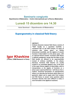
end of the century and in the following one: in 1698, Thomas Savery patented a
device that, with the use of steam, could pump water from a lower to a higher
level in order to solve water ooding problems in mines. Successively, around
1710, Thomas Newcomen developed Savery's invention by adding a piston and
1.1.
A BRIEF HISTORY OF THERMODYNAMICS
3
a cylinder to better exploit the condensation of steam in order to pump water.
The following signicant step came in the second half of the XVIII century when
James Watt introduced two improvements on Newcomen's machine: the external
condenser, that increased the eciency of the machine, and rotary motion, replacing the alternating one of the previous devices, thus reducing the stresses on the
components [Th02]. For a detailed history of the progress in steam engines and
a characterization of the great minds that have made improvements in this eld
possible, we refer to the book written by Thurston, the rst professor of Mechanical Engineering at Stevens Institute of Technology and, successively, Director of
Sibley College at Cornell University [Th02].
Fig. 1.1: Illustration of Thomas Savery's Engine of 1698.
1.1.3 Theoretical evolution of the subject
Even though practical devices, starting from the XVII Century, had been constantly improved, the theoretical knowledge regarding these processes was still
anchored to the concepts of phlogiston, a mysterious substance released during
combustion, and caloric, a uid transferring from hotter bodies to colder bodies.
Starting from the '700s, however, some scientists began to suggest that the concept
of heat was related to the movement of particles inside a body, thus assuming that
4
CHAPTER
1.
THERMODYNAMICS IN PHYSICS AND ENGINEERING
it was a form of energy.
The rst systematic study of the causes underlying the previously cited phenomena was conducted by Sadi Carnot in 1824 in his Réexions sur la Puissance
Motrice du Feu et sur les Machines Propres à Développer Cette Puissance (Reections on the Motive Power of Fire). As underlined in the preface by the editor,
Robert H. Thurston, in the 1897 publication of Carnot's work, the young French
scientist rst introduced many ideas that are at the base of modern thermodynamics. The goal of his book, very simple from a mathematical standpoint, was,
on one hand, to understand what was the maximum possible amount of work that
could be extracted from a given quantity of heat and, secondly, if this amount of
work was independent of the particular substance used in the machine. In answering these questions, he introduced the idea of a sort of conservation principle
for the motive power of heat, thus giving an embryonic idea of the Second Law
of Thermodynamics. Then, he introduced the concepts of cycle, stating that, in
order to actually evaluate the eects of a process on the environment, the process
itself must return to the initial point, and, nally, he introduced the notion of
reversibility, associated to the perfection of the cycle [Car97]. The answers to the
questions that had given birth to the book are the principles that underlie the
statement of the Second Law of Thermodynamics in its traditional formulation:
there is a maximum amount of work that can be extracted from a given quantity of heat, depending on the temperatures of the hot and cold source, and this
amount is independent of the nature of the particular substance that is used in
the machine.
From the investigation of a problem of `engineering economics', thermodynamics has grown into a body of doctrine of profound philosophical signicance [W52],
even though, as Callen evidences in the preface to his monumental book, thermodynamics was the last branch of classical physics to be reformulated from a
theoretical standpoint. This was caused by the fact that thermodynamics has
always been strongly linked to macroscopic observations, as the deep nature of
the phenomena that it investigated, related to the molecular theory of matter,
remained rather obscure for a long time. This is also the reason why its original
formulation had been developed in terms of cycles and transformations and only
successively its structure was overhauled and restated in terms of state functions
and equilibrium states, generating a simplication from a mathematical standpoint [Cal60]. However, we feel that still nowadays the theoretical structure of
thermodynamics is very much debated and a general view shared by the majority
1.2.
MAIN PROBLEMS IN THERMODYNAMICS
5
of scholars does not exist.
What we claim is particularly important to understand from the development
of the history of thermodynamics is that, with respect to other disciplines, such
as electromagnetism, it has always been more tightly linked with practical applications and results. This fact, united with the absence of a universally shared
theoretical structure and with the fact that the chemical and mechanical industries, two sectors that strongly contributed to technological and economic progress
in the XX Century, heavily rely on thermodynamics, has caused a wider engineering presence in a eld that should be a prerogative of physicists. With the present
work, as engineers that are developing a topic with strongly theoretical features,
we are thus just joining what has been a mainstream tendency in the history of
the discipline.
1.2 Main problems in Thermodynamics
After having explained the etymology of the word thermodynamics, briey illustrated its history and, most important, pointed out why we, as engineers, are
working in this eld, in the present section we aim at clarifying some basic concepts in thermodynamics, which will be helpful to understand the exact place of
our thesis topic in the more general picture of the discipline.
Recalling Albert Einstein in [Ei79], we introduce the subject by stating:
A theory is the more impressive the greater the simplicity of its
premises, the more dierent kinds of things it relates, and the more
extended its area of applicability. Therefore the deep impression that
classical thermodynamics made upon me. It is the only physical theory
of universal content which I am convinced will never be overthrown,
within the framework of applicability of its basic concepts.
The quote by the man who was probably the most prominent scientist of the
XX Century introduces to the problem of the exact positioning of thermodynamics
among the various branches of physics and its relationship with Mechanics. The
issue is still very much controversial and our aim is just to sketch the prevalent positions and to point out the view through which we were introduced to the subject,
which we found illuminating because of its clarity, sequentiality and rigour, even
though it is not one of the mainstream ways to introduce students to thermodynamics. After that, we will briey illustrate kinematics and dynamics as branches
6
CHAPTER
1.
THERMODYNAMICS IN PHYSICS AND ENGINEERING
of thermodynamics: with the rst word, we refer to the description of the possible
or allowed states of a system
[GB05], while, with the second one, we refer to a
causal description of the time evolution of a state
[GB05].
1.2.1 Epistemology
As it has been evidenced in the previous paragraph, thermodynamics was born
from a theoretical point of view thanks to the work of Carnot at the beginning
of the XIX Century. Many other scientists, most notably James Clerk Maxwell,
Ludwig Boltzmann and Josiah Willard Gibbs, contributed to changing the interpretation of the discipline and, most important, linking it with microscopic phenomena. In particular, one of the most common views of thermodynamics, based
on the ideas of Statistical Mechanics, is that of thermodynamics as a statisti-
cal science. It is based on the realization that the description of a macroscopic
system cannot be conducted by describing the evolution of all its constituents because it would lead to a practically unsolvable system of equations and variables.
As a consequence of this, thermodynamics provides a sort of eective `synthesis' of
the behaviour of a huge number of microscopic particles at the macroscopic level.
As Glansdor and Prigogine have stated, thermodynamics provides a
scription
or
simplied language
reduced de-
to describe macroscopic systems [GP71]. It can
thus be said that the statistical interpretation arises because of the impossibility
to describe the system deterministically starting from the equations of motion of
the single particles.
However, statistical foundations of thermodynamics intended in this sense have
given birth to more radical interpretations, such as those suggested by its merging
with Information Theory. The information-theoretic interpretation of the discipline suggests that the thermodynamic state of a system does not depend only
on the system itself, but also on the knowledge that the observer has: based on
this knowledge, the observer may assign probability values to the possible states of
the system and the actual conguration of the system (i.e. the actual probability
values assigned to each state) is the one that maximizes a certain function, the
entropy, as dened by Shannon ([Sha48; Ja57; Ka67]).
However, this interpretation would suggest that the actual state of the system
is not univocally determined as the maximization process is constrained by the
actual knowledge of the observer. This goes against common intuition as macroscopic phenomena are characterized by the same patterns independently of the
1.2.
MAIN PROBLEMS IN THERMODYNAMICS
7
particular observer. Moreover, the statistical interpretation of thermodynamics
poses another signicant problem: how is it possible that, in its macroscopic description, nature has a precise direction (irreversible phenomena exist), while the
microscopic equations of motion are perfectly invariant under time-reversal? Many
scientists have tried to give an explanation to this: one of the most common is
the one that claims that macroscopic laws are valid on average and the fact that
nature does not go back in time is due to the reason that it is highly improbable (it would happen probably one time during the life of the Universe), but not
impossible.
The approach of the Keenan School is radically dierent. With this name, we
refer to the School of Thermodynamics of the Massachusetts Institute of Technology (MIT), started with the pioneering work of Joseph Keenan, which brings an
unconventional and often challenged view to the subject. The work of the founder
has then been carried on by several authors during the second half of the XX
Century; among these, there are Elias P. Gyftopoulos and Gian Paolo Beretta,
whose work is frequently cited in the present thesis. According to the scholars of
the Keenan School, Thermodynamics is a non-statistical science that applies
to both micro and macro systems. An observer has no role in the interpretation
of macroscopic phenomena and irreversibility is not a feature that depends on the
particular level of description that is adopted (i.e., it exists at the macroscopic
level, but does not exist at the microscopic level), but exists on all levels. The
general results of this new approach to the discipline may be summarized in the
following main points:
• Thermodynamics is an extension of Mechanics, as the states of Mechanics are
zero-entropy states for thermodynamics; this is witnessed by the following
quotation from Gyftopoulos and Beretta:
Were we to assume that a system is subject only to the laws of
mechanics, we would conclude that all the energy of the system in
excess of the ground-state energy can be used to lift a weight. [...]
But this conclusion is not consistent with all experimental results.
[...] To account for these experiences, the laws of thermodynamics
entail a greater variety of states than contemplated by the laws of
mechanics.
The contrast between the values of the adiabatic availability in
mechanics and in general is yet another way to present the fun-
8
CHAPTER
1.
THERMODYNAMICS IN PHYSICS AND ENGINEERING
damental dierences between the domain of validity of the laws of
mechanics and that of the laws of thermodynamics, which includes
the domain of mechanics as a special and limiting case. [GB05,
p. 81]
• the consideration is valid also on the microscopic level, as more general
quantum states than those considered by Quantum Mechanics are said to
exist; this is related to the fact that the existence of entropy implies a new
paradigm 1 , as illustrated in the following quotation:
The possibility for entropy to be created by irreversibility reects
a physical phenomenon that is sharply distinct from the great conservation principles that underlie the description of physical phenomena in mechanics. It brings forth the need to consider not only
properties that are conserved, such as energy, mass, momentum,
and electric charge, but also properties that may be spontaneously
created, such as entropy.
In fact, even the requirement of entropy conservation in reversible
processes of isolated systems introduces a radical departure from
the description of physical phenomena in mechanics, a departure
that would persist even if no process in nature were irreversible.
The reason is that this requirement brings forth the need to describe not only states with zero entropy, such as the states encountered in mechanics, but also states with various nonzero values of
entropy. [GB05, p. 106]
• as irreversibility is a built-in characteristic of nature, the microscopic equations of evolution are not complete because they are time-reversible; a new
equation of motion, that has Schrodinger's equation as a particular case, is
thus needed and has indeed been proposed [Bere81].
In the following Fig. 1.2, a typical energy-entropy graph showing all the states
of thermodynamics is illustrated. It may be understood in which sense Thermodynamics is considered as an extension of Mechanics: the states of Mechanics are
1 The word
paradigm, in this context, has the same meaning that Kuhn gave it in his 1962
The Structure of Scientic Revolutions, where he challenged the consolidated view
according to which science proceeds by accumulation, replacing it with the idea that periods
of normal science are alternated with periods of revolutionary science, characterized by the
presence of new paradigms. These are the set of practices that dene a scientic discipline at
masterpiece
any particular period of time [Ku62].
1.2.
MAIN PROBLEMS IN THERMODYNAMICS
9
zero-entropy states in which all the energy of the state in excess of the state of
minimum energy may be `used to lift a weight', i.e., may be converted to work.
This would not happen starting from an isolated, non zero-entropy state because
reaching the state of minimum energy would be impossible without decreasing
the value of the entropy. It may thus be understood that evolution in Mechanics
takes place only vertically on the line of zero-entropy states, while evolution in
thermodynamics takes place in the whole graph; moreover, for each value of the
energy, Thermodynamics considers one stable equilibrium state and innite nonequilibrium states, while Mechanics is characterized by the existence of only one
state for each value of the energy and this state is a non-equilibrium state, unless
it is the one of lowest energy.
Fig. 1.2: Energy versus entropy graph: states on the continuous line are thermodynamic stable equilibrium states, while states inside the curve are non-equilibrium
states.
1.2.2 Kinematics
As it has been stated by Gyftopoulos and Beretta, kinematics is the branch
of physics that has the
description of the states of a system
as the object of
its study [GB05]. This applies in general to all the disciplines included in the
broad range of physics, thus also to thermodynamics. Fundamental in the previous
10
CHAPTER
1.
THERMODYNAMICS IN PHYSICS AND ENGINEERING
sentence is the concept of state : among the dierent denitions, we chose the
concise and qualitative one given by the same authors, who dene the state as the
set that species everything about a system at one instant of time
[GB05]. For a
wider and more rigorous denition of state, we refer to Beretta and Zanchini who,
in presenting a logical scheme that rigorously denes entropy, also give careful
operative denitions of many of the basic concepts needed to face the study of
thermodynamics; in addition to state, also system, property, environment, process,
isolated system and other concepts are given [BZ].
The key aspect thus becomes the choice of all the variables that may allow the
specication of all the information about a system at a precise instant of time.
The choice of the variables depends on the particular level of description that is
chosen for the system under consideration. This is related to the fact that dierent systems may be described with dierent degrees of coarseness. The various
levels of description have a hierarchical structure and are characterized by dierent conservation laws: in particular, a level L1 is called deeper than a level L2 if
all the constituents of L1 are conserved in the physical process under examination, while this is not true for the constituents of L2 [BZ]2 . The switch from a
lower level of description to a higher level of description is done through coarsegraining procedures, which may be seen as a sort of averaging over microscopic
states [Ö05]. Coarse-graining procedures inuence both the kinematics and the
dynamics of a physical system because, in the passage between dierent levels of
description, both the variables used to describe the system and its evolution features change. Regarding these procedures, an interesting epistemological question,
currently debated by scholars, arises: is it true that, by the successive application
of coarse-graining schemes, the researcher distances himself more and more from
the actual functioning of nature, that is from natural laws, and widens the space
allocated to the modelling part, that he himself provides?
The topic of the choice of variables is thus particularly signicant. In Equi-
librium Thermodynamics , the dierent frameworks used to build the theoretical
construct have all agreed upon the fact that, under some restrictive hypotheses,
the intensive thermodynamic stable equilibrium states may be determined through
two intensive, independent variables. That is, all the other intensive variables of
the system are univocally determined once two of them have been chosen. A third
variable is needed to scale the dimensions of the system. In general, however, if
particular hypotheses on the system are not assumed, the number of independent
2 Constituents may be seen as the elementary building blocks of matter [BZ]
1.2.
MAIN PROBLEMS IN THERMODYNAMICS
11
properties in a basis used to describe the state is innite and, thus, the choice of
the variables is much harder [GB05]. Particularly hard is thus the choice of the
variables for non-equilibrium systems.
It is not in our intention to review all the solutions that have been adopted in
the past decades in the study of non-equilibrium phenomena. However, we would
like to cite some of the most signicant ones in order to oer to the reader ideas
for possible answers to the problem and to highlight the spirit that underlies these
solutions. Classical Non-Equilibrium Thermodynamics, which will be extendedly
exposed in the second chapter of the work, considers the same variables that
characterize equilibrium thermodynamics. The additional variables that may be
considered for non-equilibrium systems may be of several dierent types; among
these, there are time derivatives of equilibrium variables, spatial uxes and internal
variables related to the structure of the system. The choice may depend, on one
hand, on the time scales that are considered and, on the other hand, on the
particular interests of the observer [Jo13]. As for the time scale, for example,
the interest is usually on degrees of freedom of the system whose relaxation times
are comparable to the rates of external perturbations. Indeed, slower degrees of
freedom will be considered frozen, while faster degrees of freedom will be assumed
as instantaneously reaching equilibrium ([JR11; LJC92; LVR01]). On the other
hand, for example, if the interest of the observer is on steady states, rates of change
would be of little use and uxes would be much more appropriate variables.
Regarding this last aspect, the class of non-equilibrium theories that considers
the uxes as independent variables for the denition of a state is called Extended Ir-
reversible Thermodynamics . Indeed, EIT adds the uxes of the conserved densities
of Classical Non-equilibrium Thermodynamics (CNET), i.e. mass and energy ux,
to the set of basic independent variables in order to better describe high-frequency
or short-wavelength phenomena (hyperbolic equations of evolution, with nite
propagation speeds, are obtained in this way, oppositely to parabolic equations
obtained through classical constitutive laws). CNET equations are obtained in
the limit of slow phenomena. Further generalization and wider domains of validity
are then obtained by adding higher-order uxes (see, e.g., [JCL88; LVCJ98]).
1.2.3 Dynamics
Dynamics is dened generally as the branch of physics that has the causes of
motion and the analysis of their eects as the objects of study [GB05]. Motion
12
CHAPTER
1.
THERMODYNAMICS IN PHYSICS AND ENGINEERING
is intended as the change in state of a system in time and is due to the presence
of external or internal forces [GB05]. In order to describe the dynamical evolution
of a system, equations of motion are needed: for example, in Classical Mechanics,
Newton's Law, relating the force acting on a body and its acceleration, describes
the dynamical features of the system, while in Quantum Mechanics, the time
evolution is depicted by the Schrödinger's Equation. In thermodynamics, such a
law is still lacking and the topic is the subject of research [GB05]. According to
Gyftopoulos and Beretta, whose view we would like to adopt in the present thesis,
even though a precise equation of motion has not been found yet, general features
that characterize this equation have been discovered and are represented by the
First and Second Law of Thermodynamics. As a consequence of this, if an equation
were discovered which describes the motion of the system in state space (without
discussing if and to what extent could the equation be used in practical terms to
calculate motions of complex systems), the two Laws could be straightforwardly
derived from it as theorems. Many attempts have been made towards this goal,
but no unquestionable result has been obtained yet.
Among these attempts, one of the most recent and, probably, most ambitious
is the one proposed by Adrian Bejan, professor of Mechanical Engineering at Duke
University [CLaw]. He has proposed the Constructal Law of Evolution as an
additional self-standing law to the already existing Laws of Thermodynamics.
He claim that the Constructal Law is a general law of physics that applies to all
ow systems, both animate and inanimate and is stated as follows:
For a nite-size ow system to persist in time (to live), its conguration must evolve in such a way that provides greater and greater access
to the currents that ow through it [CLaw]
Bejan claims that neither of the two Laws of Thermodynamics take into account design or optimization phenomena, thus the Constructal Law is needed to
consider the time evolution of a thermodynamic system (even though its application is asserted to be much more general). The narrower optimality principles
and patterns that are found both in thermodynamics and in other elds of human
experience, such as biology, technology or society, are seen as particular realization
of the more general law.
Among the other principles that have been proposed to satisfy the need of an
equation of motion for a thermodynamic system, one of the most studied is the
1.2.
MAIN PROBLEMS IN THERMODYNAMICS
13
Maximum Entropy Production Principle (MEPP). The principle has been
proposed by several authors working independently and may be stated as follows:
By this principle, a nonequilibrium system develops so as to maximize
its entropy production under present constraint. [MS06, p. 3]
The reader must be warned about the fact that great confusion upon the hypotheses at the base of this principle and upon its actual statement and meaning
is still present nowadays in the scientic community: this general expression is
often used in dierent contexts where dierent constraints and dierent optimized
variables are present. One of the purposes of the present work is the one of rationalizing part of the enormous amount of work that has been done on this topic in
order to understand the actual signicance of the principle. Moreover, the MEPP
must not be confused nor assumed to be in contrast with another principle that
has been stated to rule the evolution of non-equilibrium thermodynamic systems:
Prigogine's Minimum Entropy Production Principle [GP54]. Indeed, as it will be
illustrated during the course of the work, Prigogine's principle is, on one hand, a
global principle related to the asymptotic time evolution of the entropy production
and, on the other hand, it is valid under more restrictive hypotheses. The Maximum Entropy Production Principle is instead a principle related to the evolution
of a system at a xed instant of time and may be considered much more general:
indeed, Prigogine's principle may be considered as a consequence of MEPP under
particular restrictions. The dierence will be claried during the course of the
work.
Closely related to the principle of Maximum Entropy Production is the Steepest Entropy Ascent (SEA) dynamical model proposed by Beretta, initially in
a quantum framework and successively adapted to meso- and macroscopic systems [Bere13]. Also Grmela and Öttinger have proposed a GENERIC (General
Equation for Non-Equilibrium Reversible Irreversible Coupling), that is, an equation that describes the dynamical evolution of non-equilibrium systems at various scales [GÖ97]. The study of this dynamical model (and its relationship with
other maximum-entropy-producing principles) is included in the goals of the thesis. Many other models and theories of dynamical evolution for a thermodynamic
system have been developed and might be cited, but we will omit them, as the
purpose of the present paragraph is just sketching the borders of the topics that
will be developed in the thesis work, that is, dynamical models for thermodynamic
systems, and not reviewing the scientic literature in the eld.
14
CHAPTER
1.
THERMODYNAMICS IN PHYSICS AND ENGINEERING
1.3 Non-Equilibrium Thermodynamics
1.3.1 Non-equilibrium Thermodynamics and Engineering
As it was said in the previous paragraph, the general focus of the present work
will be on the dynamical modelling of thermodynamic systems. The subject is a
frontier topic in the eld of physics and the reader is perfectly legitimated to wonder
the reason why the present topic is debated in an engineering thesis. A partial
answer resides in what was exposed in the paragraph regarding the history of
thermodynamics: for various reasons, developments in this discipline, much more
than in other branches of physics, have been due to the work of engineers, even
from a theoretical standpoint. However, a much deeper reason is indeed present
and has a typical engineering feature: usefulness. The research for the patterns or,
more ambitiously, the equation of dynamical evolution of thermodynamic systems
is not only a challenging conceptual problem whose answer would be a milestone
for Theoretical Physics, but it would also be an extremely advantageous device
to better comprehend, govern and exploit practical phenomena. Among these,
there are thermodynamic phenomena of relaxation towards equilibrium from nonequilibrium states, which characterize an enormous number of engineering systems
of practical use. These phenomena are indeed the object of study of a wide branch
of physics, called Non-Equilibrium Thermodynamics or Thermodynamics
of Irreversible Processes, as processes of evolution from non-equilibrium states
are usually characterized by entropy production. Non-equilibrium thermodynamics
diers from equilibrium thermodynamics or thermostatics because of the need of
modelling systems that change in time. Indeed, the latter focuses on systems
having a xed state, independent of time, or systems undergoing very slow (quasi-
static ) transformations [Cal60]. As it has been stated by de Groot and Mazur, the
eld of non-equilibrium thermodynamics provides us with a general framework
for the macroscopic description of irreversible processes [dGM84]. However, it
must be evidenced that most of the consolidated work in this eld has been done
on the linear approximation for near-equilibrium states. Further details on the
meaning of linear approximation will be given in Chapter 2. It may thus be
said that far-equilibrium states and nonlinear behaviour have been excluded from
traditional treatise, even though they are key to many technological applications
[Ö05]; as a consequence of this, there is the need to have a unied approach
to nonlinear irreversible thermodynamics, the existence, necessity, and usefulness
1.3.
NON-EQUILIBRIUM THERMODYNAMICS
15
of which has currently not been fully realized by large fractions of the science
and engineering communities [Ö05]. On the other hand, from a more theoretical
standpoint, the same author claims that a unied approach would provide a deeper
understanding of beyond-equilibrium systems by oering a general framework for
dierent empirical applications, consistency with experimental results and recipes
for going from more detailed to less detailed levels of description [Ö05].
1.3.2 Potential applications
As it has been hinted at in the previous subsection, the spectrum of non-equilibrium
situations is extremely wide and very broad is also the range of practical situations
modelled through Classical Non-Equilibrium Thermodynamics and Kinetic Theory. Moreover, dynamical principles such as the Maximum Entropy Production
Principle have been adapted and used in a variety of disciplines, distant from pure
thermodynamics. Below is a list of the practical situations related to the topics
that have been cited: some of the them will be further analysed in the following
Chapters.
• A typical non-equilibrium process is the relaxation towards a stable equilibrium state of a system that has undergone a chemical reaction of oxidation,
as it happens in the vast majority of power system used nowadays by man: a
deeper knowledge of this process of evolution towards equilibrium may thus
allow to reduce the entropy generated by irreversibility during the process
and to improve the eciency of thermal machines. In Fig. 1.3, an illustration of dierent processes of evolution towards equilibrium from the initial
non-equilibrium condition are shown in an enthalpy-entropy graph: fuel-cell
oxidation generates less entropy than ame combustion, thus allowing the
extraction of a greater amount of work.
• Dynamical evolution models for far-equilibrium situations are also needed
for the description of natural phenomena for which Navier-Stokes description fails: in these situations, Kinetic Theory and, in particular, the Boltzmann Equation describe the evolution of the system, even though, in order
to simplify computations, Model Equations, usually based on strong assumptions, are used in calculation programmes. A dynamical evolution equation
for a thermodynamic system might improve the description of relaxation towards equilibrium in these contexts: one of the purposes of Steepest-EntropyAscent dynamics is exactly this one, as it will be shown in the last part of the
16
CHAPTER
1.
THERMODYNAMICS IN PHYSICS AND ENGINEERING
Fig. 1.3: Dierent evolutions towards equilibrium in an enthalpy-entropy graph
from the same non-equilibrium initial condition: oxidation in a fuel cell compared
with ame combustion.
thesis. As illustrated in Fig. 1.4, various situations of practical interest are
characterized by the failure of Navier-Stokes modelling: this happens when
the internal scale of the uid λ approaches the characteristic scale of the ow
L, that is, when the Knudsen number Kn = λ/L is signicantly dierent
from zero. Indeed, when the Knudsen number is close to zero, transport is
collision-dominated and Navier-Stokes equations are adopted; as the uid
internal scale approaches the characteristic lengthscale of the ow, NavierStokes equations remain valid only in the bulk of the ow and, eventually, as
the Knudsen number gets even higher, they have to be replaced by ballistic
motion and kinetic models. Recent work on a possible application was done
by Diab and Lakkis, who studied the behaviour of a rareed gas lm under
an oscillating micro-cantilever RF (Radio Frequency) switch [DL12].
• Typical applications of non-equilibrium thermodynamics in its classical linear approximation is the modelling of thermoelectric and thermodiusive
1.4.
STRUCTURE AND SCOPE OF THE THESIS
17
Fig. 1.4: Classication of physical phenomena according to the Mach number
and the Knudsen number, with domains of validity of the dierent equations.
processes: further details will be given in the exposition of the Classical
Non-Equilibrium theory in Chapter 2.
• Maximum-entropy production evolution principles are applied not only in the
strictly thermodynamic eld, but also in many other scientic problems and
even in the social studies sphere. Citing a few examples, maximum-entropy
production models have been applied to climate studies by Paltridge, who
showed that the Earth's atmosphere is seemingly characterized by maximum
dissipation processes related to horizontal energy ows [Pa79]; Juretic and
Zupanovic have modelled steady-state bacterial photosynthesis concluding
that photosynthetic proton pumps operate close to the maximum-entropy
production mode [JZ03]; Shizawa and Zbib developed a thermodynamic
theory of elastoplasticity, introducing a dislocation density tensor on the
basis of the principle of maximal entropy production rate [SZ99].
1.4 Structure and scope of the Thesis
After having dened the general topic that frames the thesis, the illustration of its
scopes and its structure may be more clear.
18
CHAPTER
1.
THERMODYNAMICS IN PHYSICS AND ENGINEERING
1.4.1 Goals of the Work
The main goals of the present work are the following:
• rst of all, some Maximum-Entropy-Production dynamical models for NonEquilibrium Thermodynamics, elaborated during the course of the last decades,
will be presented and systematically reviewed, introducing then the Steepest
Entropy Ascent dynamical model, recently adapted by Beretta to meso- and
macroscopic systems [Bere13];
• the Steepest Entropy Ascent (SEA) dynamical model, which aims at geometrizing the dynamic evolution of a thermodynamic system, is then compared with one of the most renowned presentations of metriplectic dynamics,
aimed at a geometrization of Non-Equilibrium Thermodynamics, that is, the
GENERIC (General Equation for Non-Equilibrium Reversible-Irreversible
Coupling) formalism, developed, among others, by Grmela and Öttinger in
the last two decades of the XX Century [GÖ97]: a comparison between the
two models, both motivated by the search for Non-Equilibrium Thermodynamics formulations that are fully compatible with the Second Law, with
the identication of similar and dierent features, will be conducted;
• nally, in order to have a clearer comprehension of the two dynamic models,
their compatibility with Classical Non-Equilibrium Thermodynamics will be
evaluated and their realization in Kinetic Theory will be illustrated, with a
numerical example of the use of a Steepest Entropy Ascent kinetic model for
the Boltzmann Equation to reproduce the relaxation from a highly nonequilibrium state, as recently studied by Beretta and Hadjiconstantinou
[BH13].
1.4.2 Organization of the Work
The structure of the thesis is listed as follows.
• Chapter 2 will be devoted to the explanation of the classical consolidated
theories used to test the successively illustrated models; rstly, Classical NonEquilibrium Thermodynamics (CNET), formalized by de Groot and Mazur
in their best-selling physics book [dGM84], and linear approximations of
non-equilibrium phenomena, with particular reference to Onsager's theory,
1.4.
STRUCTURE AND SCOPE OF THE THESIS
19
will be explained; then, a general introduction to Kinetic Theory and to the
Boltzmann Equation will be given.
• Chapter 3 will be dedicated to the illustration of some of the MaximumEntropy Production Principles (MEPP) that have been developed in the
history of thermodynamics, with particular reference to the theory developed
by Ziegler [Zi57], and to the explanation of their relationship with CNET;
the Steepest Entropy Ascent (SEA) model will then be introduced; in the
second part of the chapter, theoretical studies conducted by Bataille, Edelen,
and Kestin [BEK79] will be illustrated, paying particular attention to the
introduction of the idea of the two-generator formalism, which is also used
in the GENERIC structure.
• Chapter 4 will be devoted to the illustration of the Classical Mechanics equations in the Dierential Geometry framework; indeed, as it has been exposed
by Marsden and Ratiu [MR03], Dierential Geometry is the most natural
setting of the classical Lagrange and Hamilton equations and some peculiar
structures used in this modelling are then at the base of the GENERIC formalism developed, among others, by Grmela and Öttinger [GÖ97], which is
successively illustrated in the chapter. The second part of the Chapter constitutes the most innovative output of our thesis work: Dierential Geometry
has been considered to be the most appropriate setting in which a comparison
of the Steepest Entropy Ascent dynamical model and the GENERIC formalism may be conducted. Because of this, SEA has been translated into
Dierential Geometry terms and, following this reformulation, it becomes
clear that the GENERIC formalism adopts an entropy-gradient dynamics,
such as the one proposed in SEA, with the dierence that it is built in
a more structured environment. Considerations on the relationship among
SEA, GENERIC and the models explained in the previous chapters will then
be illustrated.
• Chapter 5 will be devoted to the illustration of the applications of the two
models. First of all, the interpretation of the equations of Hydrodynamics and Magnetohydrodynamics (MHD) in the GENERIC formalism will be
shown. Then, the realization of SEA and GENERIC in Kinetic Theory will
be illustrated. The dierent terms of the Boltzmann equation may be associated to the dierent building blocks of the two theories. In particular,
20
CHAPTER
1.
THERMODYNAMICS IN PHYSICS AND ENGINEERING
the metrics that are used will be discussed. Finally, a numerical example
of Steepest Entropy Ascent relaxation from a highly non-equilibrium state,
recently developed by Beretta and Hadjiconstantinou, will be illustrated and
comments will be made on the eectiveness of the model equation thus obtained, compared with those that are normally used [BH13].
• Chapter 6 will be dedicated to the conclusions and future developments and
it will be followed by two Appendices. The rst one contains a Compendium
of Dierential Geometry; we indeed felt that this Appendix was necessary
in order to introduce the reader to the basic concepts and formalism used
to reformulate SEA dynamics as they are not usually found in a standard
engineering Master of Science course. The second Appendix is much shorter
and aims at explaining the mathematics underlying Edelen's theory, exposed
in Chapter 3, related to the so-called Helmholtz-Hodge decomposition.
We warn the reader used to a typical engineering treatise that the second part of
the thesis may, at rst sight, be found particularly heavy and hard to understand,
especially because of the Dierential Geometry mathematical formalism that is
usually not taught in regular curricula. Because of this, we made a strong eort
of always trying to anticipate through physical or geometric intuition the general
meaning of the mathematical expressions that we would have successively introduced. However, we felt that this formalism was strictly necessary: if the reader
deeply comprehends it, he will clearly understand that it is the most natural and
limpid setting of the dynamical modelling of thermodynamic systems.
CHAPTER
1.
REFERENCES
21
References
[BEK79]
J. Bataille, D. G. B. Edelen, and J. Kestin. On the structuring of thermodynamic uxes: a direct implementation of the dissipation inequality.
In: International Journal of Engineering Science 17.5 (1979), pp. 563572
(cit. on p. 19).
[Bere13]
G. P. Beretta. Steepest-Entropy-Ascent and Maximal-Entropy-Production
Dynamical Models of Irreversible Relaxation to Stable Equilibrium from
Any Non-Equilibrium State. Unied Treatment for Six Non-Equilibrium
Frameworks. In: Proceedings of the 12th Joint European Thermodynamics
Conference, JETC 2013. Ed. by M. Pilotelli and G. P. Beretta. Brescia:
Cartolibreria Snoopy, 2013, pp. 100109 (cit. on pp. 13, 18).
[Bere81]
G. P. Beretta. On the general equation of motion of quantum thermodynamics and the distinction between quantal and nonquantal uncertainties.
thesis. 1981 (cit. on p. 8).
[Berg06]
S. Berger. A Companion to Nineteenth-century Europe. Blackwell, 2006
(cit. on p. 2).
[BH13]
G. P. Beretta and N. G. Hadjiconstantinou. Steepest Entropy Ascent Models of the Boltzmann Equation. Comparisons with Hard-Sphere Dynamics
and Relaxation-Time Models for Homogeneous Relaxation from Highly
Non-Equilibrium States. In: Proceedings of the ASME 2013 International
Mechanical Engineering Congress and Exposition, IMECE 2013. 2013 (cit.
on pp. 18, 20).
[Bo00]
J. Bolton. Classical Physics of Matter. CRC Press, 2000 (cit. on p. 2).
[BZ]
G. P. Beretta and E. Zanchini. Rigorous and General Denition of Thermodynamic Entropy. In: Thermodynamics. Ed. by M. Tadashi. InTech,
2011, pp. 2350 (cit. on p. 10).
E. Zanchini and G. P. Beretta. Rigorous operational denition of entropy
not based on the concepts of heat and of empirical temperature. In: Pro-
ceedings of the 12th Joint European Thermodynamics Conference, JETC
2013. Ed. by M. Pilotelli and G. P. Beretta. Brescia: Cartolibreria Snoopy,
June 2013, pp. 152159. Cit. on p. 10.
22
[Cal60]
CHAPTER
1.
THERMODYNAMICS IN PHYSICS AND ENGINEERING
H. B. Callen. Thermodynamics: an Introduction to the Physical Theories
of Equilibrium Thermostatics and Irreversible Thermodynamics. New York:
John Wiley & Sons, 1960 (cit. on pp. 4, 14).
[Car97]
N. L. S. Carnot. Réexions sur la Puissance Motrice du Feu et sur les
Machines Propres à Développer Cette Puissance (Reections on the Motive
Power of Fire). Ed. by R. H. Thurston. 2nd ed. New York: John Wiley &
Sons, 1897 (cit. on pp. 4, 6).
[CLaw]
A. Bejan. Constructal-theory network of conducting paths for cooling a
heat generating volume. In: International Journal of Heat and Mass Trans-
fer 40.4 (1997), pp. 799816 (cit. on p. 12).
A. Bejan and S. Lorente. The constructal law and the thermodynamics
of ow systems with conguration. In: International Journal of Heat and
Mass Transfer 47.14-16 (2004), pp. 32033214 .
A. Bejan and S. Lorente. Constructal law of design and evolution: Physics,
biology, technology, and society. In: Journal of Applied Physics 113.15
(2013). Cit. on p. 12.
[CT04]
Y. A. Cengel and R. H. Turner. Fundamentals of Thermal-Fluid Sciences.
McGraw-Hill, 2004 (cit. on p. 2).
[dGM84]
S. R. de Groot and P. Mazur. Non-equilibrium Thermodynamics. 2nd ed.
(1st ed., North-Holland, 1962). Mineola (New York): Dover Publications,
1984 (cit. on pp. 14, 18).
[DL12]
N. A. Diab and I. A. Lakkis. DSMC Simulations of Squeeze Film Under
a Harmonically Oscillating Micro RF Switch With Large Tip Displacements. In: ASME 2012 International Mechanical Engineering Congress
and Exposition. Houston, 2012, pp. 187197 (cit. on p. 16).
[Ei79]
A. Einstein. Autobiographical notes. A centennial edition. Ed. by P. A.
Schilpp. Chicago, Illinois: Open Court Publishing Company, 1979 (cit. on
p. 5).
[GB05]
E. P. Gyftopoulos and G. P. Beretta. Thermodynamics: Foundations and
Applications. 2nd ed. (1st ed., Macmillan, 1991). Mineola (New York):
Dover Publications, 2005 (cit. on pp. 612).
CHAPTER
[GÖ97]
1.
REFERENCES
23
M. Grmela and H. C. Öttinger. Dynamics and thermodynamics of complex
uids. I. Development of a general formalism. In: Physical Review E -
Statistical Physics, Plasmas, Fluids, and Related Interdisciplinary Topics
56.6 (1997), pp. 66206632 (cit. on pp. 13, 1819).
[GP54]
P. Glansdor and I. Prigogine. Sur les proprietes dierentielles de la production d'entropie. In: Physica 20 (1954), pp. 773780 (cit. on p. 13).
[GP71]
P. Glansdor and I. Prigogine. Thermodynamic Theory of Structure, Sta-
bility and Fluctuations. New York: Wiley-Interscience, 1971 (cit. on p. 6).
[Hay01]
D. T. Haynie. Biological Thermodynamics. 2nd ed. Cambridge: Cambridge
University Press, 2001 (cit. on p. 2).
[Ja57]
E. T. Jaynes. Information Theory and Statistical Mechanics. In: Physical
Review 106.4 (1957), pp. 620630 (cit. on p. 6).
[JCL88]
D. Jou, J. Casas-Vázquez, and G. Lebon. Extended irreversible thermodynamics. In: Reports on Progress in Physics 51 (1988), pp. 11051179
(cit. on p. 11).
[Jo13]
D. Jou. Entropy, entropy ux, temperature, and second law in extended
irreversible thermodynamics. In: Proceedings of the 12th Joint European
Thermodynamics Conference, JETC 2013. Ed. by M. Pilotelli and G. P.
Beretta. Brescia: Cartolibreria Snoopy, 2013, pp. 211216 (cit. on p. 11).
[JR11]
D. Jou and L. Restuccia. Mesoscopic transport equations and contemporary thermodynamics. In: Contemporary Physics 52 (2011), pp. 465474
(cit. on p. 11).
[JZ03]
D. Juretic and P. Zupanovic. Photosynthetic models with maximum entropy production in irrevrsible charge transfer steps. In: Computational
Biology and Chemistry 27 (2003), pp. 541553 (cit. on p. 17).
[Ka67]
A. Katz. Principles of Statistical Mechanics. The Information Theory Ap-
proach. San Francisco: Freeman, 1967 (cit. on p. 6).
[Ku62]
T. S. Kuhn. The Structure of Scientic Revolutions. Chicago: University
of Chicago Press, 1962 (cit. on p. 8).
24
[LJC92]
CHAPTER
1.
THERMODYNAMICS IN PHYSICS AND ENGINEERING
G. Lebon, D. Jou, and J. Casas-Vázquez. Questions and answers about
a thermo dynamic theory of the third type. In: Contemporary Physics 33
(1992), pp. 4151 (cit. on p. 11).
[LVCJ98]
R. Luzzi, Á. R. Vasconcellos, J. Casas-Vázquez, and D. Jou. On the selection of the state space in nonequilibrium thermodynamics. In: Physica
A 248 (1998), pp. 111137 (cit. on p. 11).
[LVR01]
R. Luzzi, Á. R. Vasconcellos, and J. G. d. P. Ramos. Statistical Foundations
of Irreversible Thermodynamics. Leipzig: Teubner, 2001 (cit. on p. 11).
[MR03]
J. E. Marsden and T. S. Ratiu. Introduction to Mechanics and Symmetry. A
Basic Exposition of Classical Mechanical Systems. 2nd ed. (1st ed., 1994).
New York: Springer-Verlag, 2003 (cit. on p. 19).
[MS06]
L. M. Martyushev and V. D. Seleznev. Maximum entropy production principle in physics, chemistry and biology. In: Physics Reports 426.1 (2006),
pp. 145 (cit. on p. 13).
[Ö05]
H. C. Öttinger. Beyond Equilibrium Thermodynamics. 1st ed. Hoboken
(New Jersey): Wiley, 2005 (cit. on pp. 10, 1415).
[Pa79]
G. W. Paltridge. Climate and thermodynamic systems of maximum dissipation. In: Nature 279 (1979), pp. 630631 (cit. on p. 17).
[Seb01]
A. Sebastian. A Dictionary of the History of Science. Taylor and Francis,
2001 (cit. on p. 2).
[Sha48]
C. E. Shannon. A Mathematical Theory of Communication. In: The Bell
System Technical Journal 27 (1948), pp. 379423, 623656 (cit. on p. 6).
[SZ99]
K. Shizawa and H. M. Zbib. A Thermodynamical Theory of Plastic Spin
and Internal Stress with Dislocation Density Tensor. In: Journal of Engi-
neering Materials and Technology 121.2 (1999), pp. 247253 (cit. on p. 17).
[Th02]
R. H. Thurston. A History of the Growth of the Steam Engine. New York:
D. Appleton and Company, 1902 (cit. on p. 3).
[W52]
L. P. Wheeler. Josiah Willard Gibbs. New Haven: Yale University Press,
1952 (cit. on p. 4).
CHAPTER
[Zi57]
1.
REFERENCES
25
H. Ziegler. Thermodynamik und rheologische Probleme. In: Ingenieur-
Archiv 25.1 (1957), pp. 5870 (cit. on p. 19).
26
CHAPTER
1.
THERMODYNAMICS IN PHYSICS AND ENGINEERING
2
Validating the model
The purpose of the present chapter is to briey present the two `theories' that will
be used to `validate' the dynamical models illustrated in the following chapters,
with particular regard to Steepest Entropy Ascent and the GENERIC formalism.
The two `theories' are Classical Non-Equilibrium Thermodynamics (CNET)
in its linear approximation and Kinetic Theory (KT). As these two `theories'
are used to model very dierent types of phenomena, we have to specify the sense
in which we aim at validating the dynamical models through them.
CNET in its linear approximation, which will be described in its main features
in the following section, has been proved to be eective in modelling so-called near
equilibrium situation, that is, situations in which the system under observation
is situated close to thermodynamic equilibrium. Its main features, which are the
linear relationship between forces and uxes and the symmetry of the matrix of
coecients that relates the rst to the second ones, must then be reproduced by
all dynamical theories, also those that aim at modelling far-equilibrium situations,
when equilibrium is approached. Thus, in the following chapters it will be shown
how these features may or may not naturally emerge in the context of SEA and
GENERIC for near-equilibrium approximations.
On the other hand, Kinetic Theory models systems characterized by a high
27
28
CHAPTER
2.
VALIDATING THE MODEL
number of particles in random motion, allowing the computation of macroscopic
properties from a statistical microscopic description. On the basis of the more or
less restrictive hypotheses that may be stated to `build' an equation governing the
time evolution of the system, dierent dierential equations for the main variable,
that is the distribution function f , may be obtained. Mathematical challenges
related to the resolution of these equations are linked to the number and type of
hypotheses that were made to obtain them. One of the most used among these
equations is the Boltzmann equation. The procedure to obtain it, its physical
meaning and the possible ways to solve it will be shown in the second part of the
chapter. The equation will then be `used' to understand how it is framed in the
SEA and GENERIC dynamical models, that is, how the dierent terms of the
equation are associated to the dierent `blocks' of the two models and how the
equation is shown to emerge naturally in the two settings. Finally, a numerical example of relaxation from a highly non-equilibrium state, using a Steepest-EntropyAscent model of the Boltzmann equation will be shown, in order to understand
the eectiveness of the dynamic theory in modelling actual situations.
The premise for the present Chapter was necessary in order to correctly frame
the following paragraphs in the more general picture of the thesis and in order to
understand that the exposition of CNET and KT is not an end in itself, but is
functional to the following parts of the work. In these paragraphs, we have made
the deliberate choice of favouring a more qualitative description of the topics,
rather than reporting numerous equations, in order to convey the main ideas to
the reader more rapidly.
2.1 Non-Equilibrium Thermodynamics
As it has been stated in the introduction, Non-Equilibrium Thermodynamics is
the branch of physics that studies systems that are not in a condition of thermodynamic equilibrium, that is, systems that cannot be described through the
relationships peculiar to thermostatics. The discipline is also called thermody-
namics of irreversible processes, as the processes of evolution towards equilibrium
from non-equilibrium situations are (almost) always characterized by the generation of entropy. Non-equilibrium thermodynamics may be considered an extension
of thermostatics towards the continuum disciplines, such as uid dynamics and
electromagnetism. Indeed, while thermostatics considers one value of the state
variables for the whole system, on the other hand, non-equilibrium thermodynam-
2.1.
NON-EQUILIBRIUM THERMODYNAMICS
29
ics considers state variables as elds that are dened for every point in space and
time [dGM84].
2.1.1 The hypothesis of local equilibrium
The fundamental assumption that resides at the base of Classical Non-Equilibrium
Thermodynamics is the hypothesis of local equilibrium, also known as hypothesis
of evolutive equilibrium. According to this assumption, the system can be divided
in many subsystems of small dimensions, each of which can be considered in a
thermodynamic equilibrium state, thus allowing the use of the fundamental relations of thermodynamics, with particular reference to the Gibbs equation. The
fundamental justication of this hypothesis lies in the validity of the results that
are obtained from its application.
However, there is a criterion that may be used to verify if the hypothesis of
evolutive equilibrium for a generic system is acceptable: the comparison between
the internal time-to-equilibrium of the system and the characteristic time of the
perturbation applied to the system. If the former is much smaller than the latter,
it means that the system reaches quickly equilibrium after a modication of the external conditions. It is thus a good approximation to use thermodynamic relations
at equilibrium. On the other hand, if the characteristic time of the perturbation
is comparable to the time-to-equilibrium of the system, the assumption loses its
physical validity because the frequency of excitation is suciently high to never
let the system reach a near-equilibrium condition.
In general, as the time-to-equilibrium of a system depends on its dimensions
(the smaller the system, the shorter the time-to-equilibrium), progressively dividing a system into many subsystems eventually leads to a time-to-equilibrium that
is much smaller than the characteristic time of the perturbation, thus making the
local equilibrium assumption reasonable. However, there is a constraint in this process: the subsystems considered at local equilibrium should contain a suciently
high number of particles. If the system were too rareed, the equations of thermostatics would not be valid. Numerically, the applicability of these equations is
veried upon the value of the Knudsen number, dened as
Kn =
λ
,
D
(2.1)
where λ is the mean free path of the particles and D is the characteristic length
30
CHAPTER
2.
VALIDATING THE MODEL
of the system under consideration. If the Knudsen number is suciently close to
zero, the system may be considered as suciently dense.
2.1.2 The entropy production term
Traditional non-equilibrium thermodynamics and most of the successive nonequilibrium theories develop starting from an observation on the form that the entropy
production term assumes after combining the various balance equations.
The fundamental balance equations in continuum physics are the mass balance,
momentum balance and energy balance equations. In non-equilibrium thermodynamics, a relevant role is attributed to a fourth equation: the entropy balance
equation. The entropy balance equation in its local formulation can be written as
follows:
∂
(ρs) = − ∇ ·j s + σs ,
(2.2)
∂t
where ρ is the mass density of the medium, s is the entropy per unit mass, js is
the entropy ux and σs is the entropy production per unit volume and per unit
time. The equation appears as a regular balance equation with a time-variation
term, a ux term and a generation term. The peculiarity is that the second law
of thermodynamics imposes that the latter must be non-negative as entropy may
only be generated and cannot be destroyed.
If the rst three, fundamental, balance equations are inserted into the Gibbs
relation, that is, the expression for the dierential of the entropy as a function of the
dierentials of internal energy, volume and concentrations, valid at thermodynamic
equilibrium, an expression for both the entropy ux and the entropy production
term may be recognized. Indeed, the resulting expression may be shown to have
the form of a balance equation:
Ds
= −∇·
ρ
Dt
jq −
P
k
µk j k
T
n
1X
−
jq · ∇ T
+
T2
r
1
µk
1X
−
j · T∇
− Fk − Π : ∇v −
Jj Aj , (2.3)
T k=1 k
T
T
T j=1
where j q is the heat ow, j k is the diusion ow of component k , µk is the chemical
potential of component k , F k is the force per unit mass exerted on component k ,
Π is the non-isotropic part of the pressure tensor and, nally, Jj and Aj are the
chemical reaction rate and the chemical anity of reaction j , respectively.
2.1.
NON-EQUILIBRIUM THERMODYNAMICS
31
Once the equation has been cast in a balance form, the ux term and the
generation term may be easily identied simply by comparison with the original
form of the entropy balance equation:
js =
jq −
P
T
k
µk j k
,
(2.4)
and
σ=−
n
r
1
jq · ∇ T
1X
1X
µk
−
F
−
Π
:
∇
v
−
−
j
·
T
∇
Jj Aj .
k
T2
T k=1 k
T
T
T j=1
(2.5)
The entropy ow term is characterized by two contributions: a term due to
the heat ow and a term due to the ow of matter. This expression is often
referred to as the heat-diusion interaction. It may also be seen from the previous
expressions that the entropy production term is given by a bilinear form: it is
the sum of the products of a ow with a conjugated force. The force, also called
anity, is either the gradient of an intensive state variable, an external force or the
dierence between thermodynamic state variables. From a physical standpoint, a
thermodynamic force quanties the gap of a certain variable from its equilibrium
value. Indeed, at equilibrium, all thermodynamic forces vanish, because there are
no gradients, nor gaps from equilibrium values of state variables. As a consequence
of this, the entropy production term goes to zero, which is its minimum value, as
it is always non-negative because of the second law of thermodynamics.
2.1.3 Linear relationships and Curie's Principle
The simplest assumption on the functional dependence of the uxes states that a
generic ux depends on the thermodynamic forces and on the thermodynamic state
variables. It can be said that this assumption is based on common sense and
reasonably simplies successive analytical developments. However, other theories
that extend the range of functional dependency to other variables have been developed. A signicant example that has already been cited in the introduction is the
one of non-local theories1 , such as the one developed by Jou, Casas-Vázquez, and
Lebon, which claim that uxes also depend on the gradients of the thermodynamic
forces [JCL10].
1 Non-local theories are theories characterized by the fact that the variables at one point in
space are not determined from
local-equilibrium relationships.
32
CHAPTER
2.
VALIDATING THE MODEL
Once the functional dependence has been set, it is the particular form of the
force-ux relation that characterizes a specic non-equilibrium thermodynamic
theory. The simplest version is a linear relationship. Linear relations between
uxes and their conjugate thermodynamic forces had already been developed, from
a strictly phenomenological point of view, in the XIX century during the study
of various physical phenomena. Among these, there are Fourier's Law for heat
conduction, Ohm's Law in electrodynamics and Fick's Law in mass transfer. The
peculiarity of these phenomenological laws is related to the fact that each ux
only depends on its corresponding force, i.e. the heat ux only on the temperature
gradient, the electric current only on the gradient of the electric potential, the
diusive ow only on the concentration gradient.
However, a thermodynamic ux may, more generally, depend on a linear combination of all thermodynamic forces. The linear relationships may thus be generalized as
Ji =
X
Lik Xk ,
(2.6)
k
However, uxes and forces have dierent dimensions: they can be scalars, vectors
or second order tensors. In the more general case, each ux depends on all types
of forces and, as a consequence of this, the linear coecients must have dierent
dimensions. The presence of particular symmetries for the medium under consideration allows a simplication of the more general dependence of each ux from
all types of forces: this is called Curie's symmetry principle [Cu08]. This proof
is based on the invariance of the phenomenological coecients, that is, the coecients relating uxes and forces (which have dierent tensorial orders), under
suitable transformations, related to the type of symmetry that is assumed for the
medium. For example, if the medium is isotropic, the phenomenological coecients
should be invariant under inversion and under all types of rotations. This leads
to the fact that, for an isotropic medium, phenomenological coecients relating
uxes and forces of dierent orders are zero and the remaining ones all depend on
a sole scalar value. This simplies the expression for the entropy production term
in the isotropic case. In the same way, simplied forms of the phenomenological
coecients may be found when the medium is supposed to be characterized by
other types of symmetries (for example, cubic symmetry imposes invariance under
inversions, 90-degrees rotations around coordinate axes and 120-degrees rotations
around body diagonals) (see Chapter 6 of [dGM84]). In the isotropic case, we have
2.1.
NON-EQUILIBRIUM THERMODYNAMICS
33
thus the following relationships between forces and uxes:
J s = Lss X s ,
(2.7)
J v = Lvv X v ,
(2.8)
J t = Ltt X t ,
(2.9)
where J are the uxes, X are the forces, the letter s stands for scalar, the letter
v stands for vector and the letter t stands for tensor. Implicit in the previous
notation are the sum signs over the dierent forces of the same tensorial order.
2.1.4 Onsager's theory
A further simplication of the system of equations that has been obtained is possible thanks to Onsager reciprocal relations [O31], which may be stated as
Lkl = Llk .
(2.10)
Considering the matrix L of phenomenological coecients, the symmetry relationships may be written as
L = LT .
(2.11)
The following paragraph will illustrate the original formulation of the proof of
the validity of Onsager's symmetry relationships, which is based on the idea of
microscopic reversibility, that is, the fact that a particle at the microscopic level
always traces back its path when its velocity is inverted.
Proof from Statistical Mechanics
The proof of the reciprocal relationships was given by Onsager in the framework
of statistical mechanics. In particular, a system of denite energy E and denite
number of particles N , obeying the micro-canonical distribution (all states comprised between energy E and energy E +dE are equally probable), is considered in
the phase space. A macroscopic description of the system can be given on the base
of n extensive variables, which compose the vector A = A(r N , pN ) that depends
on the position and momentum of each particle of the system. Because of the
motion of particles in the phase space, the values of A are subject to uctuations;
thus, their instantaneous value may be dierent from their average value and the
34
CHAPTER
2.
VALIDATING THE MODEL
following relevant quantity may be dened:
(2.12)
αi = Ai − hAi i
Thus, the vector α is the vector containing the shift of the value of the macroscopic
extensive variables from their average value (averages must be interpreted either
as time averages or as averages over a certain ensemble of systems).
Onsager's proof, which will not be illustrated, is based on several assumptions,
listed as follows.
• First of all, the probability density function f (α1 , α2 , . . . , αn ) is assumed to
have a Gaussian distribution:
1
f (α1 , α2 , . . . , αn ) = ce− 2k
P
ij
gij αi αj
,
(2.13)
where c is a normalization constant, k is Boltzmann's constant and g is a
symmetric positive denite matrix.
• Secondly, the average value of α is assumed to obey the linear dierential
equation of the rst order
∂ ᾱα0
= −M ᾱα0 ,
∂t
(2.14)
where the α0 indicates the imposed initial conditions and M is the matrix
of phenomenological coecients, independent of time. It has been experimentally proved for a wide range of conditions that this linear dierential
equation, called regression law is actually veried.
• Third, time reversal invariance of the equation of motion is considered: that
is, if the momenta of all the particles at a certain point in time and space are
inverted, the particles trace back their paths with reversed momenta. This
hypothesis leads to the property of microscopic reversibility. Even though
these properties have been proved in the framework of statistical mechanics,
they could be obtained also considering the quantum behaviour of particles.
For the sake of brevity, we omit the mathematical treatise regarding this aspect of the proof. It must also be noted that we are adopting the simplifying
assumptions of the absence of magnetic elds and the consideration of variables that are even with respect to velocity. With the presence of magnetic
2.1.
35
NON-EQUILIBRIUM THERMODYNAMICS
elds and odd variables with respect to velocity, the proof would be a little
more burdensome.
• Finally, Boltzmann's entropy postulate is adopted:
(2.15)
f (α) = f (0)e∆S/k .
This postulate relates the entropy of a generic state described by the vector
α to the entropy of the most probable state, called equilibrium state (i.e.
the state characterized by a null gap from the average values of the macroscopic variables), through the values of the microscopic probability density
distribution of the two states.
The vector X is then dened as
def
X =k
∂
ln f ,
∂α
(2.16)
and, because of Eq. 2.15, is related to the entropy as follows:
X=
∂
∆S.
∂α
(2.17)
Thus, the vector X can be interpreted as the vector of intensive thermodynamic
variables conjugated to the vector α of the extensive ones, in the same way as in
equilibrium thermodynamics the intensive state variables are the partial derivatives
of the entropy with respect to the extensive ones (for example, 1/T =
∂s
).
∂u
Based on the previous hypothesis, it can be proved that the matrix L, dened
as follows, is symmetric:
∂ α0
α = LX α0 .
(2.18)
∂t
This conclusion was the one obtained by Onsager in his papers and it shows the
validity of its reciprocal relations if we agree in considering the time derivatives of
the state variables as uxes and the quantity X as an anity. The problem of
the transfer of these relationships, obtained on a microscopical point of view, to
the phenomenological equations, whose uxes are not only time-derivatives, but
usually spatial derivatives, will be faced in the following paragraph.
Under the same hypotheses, it can be proved that the quadratic forms associated to L are positive denite; that is, for a generic vector ξ , it can be proved
36
CHAPTER
2.
VALIDATING THE MODEL
that
(2.19)
ξ T Lξ ≥ 0
In this way, the positive denite character of the entropy production, which is a
bilinear form in L, if linear relationships between forces and uxes are assumed, is
proved to hold microscopically under the previously illustrated assumptions. On
the other hand, from a macroscopic point of view, the positive denite character
of the entropy production derives from the second principle of thermodynamics
and the positive denite character of the matrix L would be a consequence of this.
The fact that, under the previously stated hypotheses, the non-negativeness of the
entropy generation is derived as a consequence may be a hint on the fact that the
assumptions are too restrictive; this would, however, call into question the validity
of the proof of Onsager reciprocal relations. Finally, it may also be proved that,
as the time goes to innity, the average value of the shift of the vector α from its
equilibrium value goes to zero:
(2.20)
lim ᾱα0 (t) = lim e−M t α0 = 0
t→∞
t→∞
Extension of Onsager relations for vectorial and tensorial phenomena
Onsager relations as derived in the statistical mechanics framework are valid for
scalar macroscopic variables (more precisely, they are valid for the dierence of
the values of these variables from their equilibrium values) and for uxes that
are time derivatives of these variables. However, macroscopic phenomenological
equations contain vectorial and tensorial variables, as well as uxes which are not
time derivatives of state variables. As a consequence of this, it is necessary to
prove that Onsager reciprocal relations are valid for phenomenological equations
too.
The rigorous proof is here omitted and only a general idea of the procedure is
given, examining the case of an isotropic uid characterized by heat conduction and
mass diusion phenomena [dGM84, p. 74]. Using the Gibbs equation, expressing
the dierential of the entropy as a function of the dierentials of the extensive
variables, and the mass and energy balance equations, the following expressions
for the total derivative of the entropy production is obtained:
dS
=ρ
dt
Z
Ω
n−1
1 ∂u X µk − µn ∂ck
∆
−
∆
T ∂t
T
∂t
k=1
!
dV.
(2.21)
2.1.
37
NON-EQUILIBRIUM THERMODYNAMICS
It must be noted that, in this Equation, and in the following Eq. 2.22, Eq. 2.23,
Eq. 2.27 and Eq. 2.28, the symbol ∆ is used to indicate a dierence and not a
Laplacian. It may be seen that the entropy production is still a bilinear form in the
forces and uxes; the rst ones are the dierences between the local value and a
generic reference value at a reference point r 0 , whereas the second ones are the time
derivatives of state variables. The sum has become an integral because it depends
on the product of forces and uxes in all points of the considered domain. Following
this interpretation and the linear structure of phenomenological relationships, the
uxes may be written as a linear combination of the forces in all points of space,
that is, as an integral:
∂u
=ρ
∂t
)
Z (
n−1
0
0
X
1
−
µ
µ
Kqq (r, r 0 )∆ 0 −
Kqk (r, r 0 )∆ k 0 n dr 0 ,
T
T
k=1
(2.22)
and
)
Z (
n−1
0
0
X
∂ci
1
µ −µ
=ρ
Kiq (r, r 0 )∆ 0 −
Kik (r, r 0 )∆ k 0 n dr 0
∂t
T
T
k=1
(i = 1, 2, . . . , n − 1).
(2.23)
For these equations, Onsager reciprocal relations are assumed to hold, except for
r = r0 and r 0 = r0 :
(2.24)
Kqq (r, r 0 ) = Kqq (r 0 , r),
Kiq (r, r 0 ) = Kqi (r 0 , r)
(i = 1, 2, . . . , n − 1),
(2.25)
Kik (r, r 0 ) = Kki (r 0 , r)
(i = 1, 2, . . . , n − 1).
(2.26)
On the other hand, by inserting the linear phenomenological equations into the
energy and mass balance equations, the following expressions may be obtained:
n−1
1 X
µk − µn
∂u
= −div Lqq ∇ ∆ −
Lqk ∇ ∆
ρ
∂t
T
T
k=1
n−1
∂ci
1 X
µk − µn
ρ
= −div Liq ∇ ∆ −
Lik ∇ ∆
∂t
T
T
k=1
!
,
(2.27)
!
(i = 1, 2, . . . , n − 1).
(2.28)
The term on the right of these equations may be written as an integral by multiplying the whole expression for a three-dimensional delta function centred in r .
38
CHAPTER
2.
VALIDATING THE MODEL
Successively integrating by parts, this integro-dierential equations takes an aspect similar to Eq. (2.22) and Eq. (2.23), allowing to identify the values of the
coecients K . Mathematical manipulation of the equalities that have been obtained lead to the proof that Onsager relations hold also for the phenomenological
coecients L, as it was originally stated in Chapter 6 of [dGM84].
The procedure used in the previous paragraph to prove that Onsager reciprocal
relationships are valid also for vectorial and tensorial phenomena on a macroscopic
point of view may not seem totally convincing. On one hand, in the specic
case that has been examined, taking into consideration only the phenomena of
heat diusion and mass diusion leads to a lack of generality; on the other hand,
however, the proof may seem to be built to suit ad hoc the formulation of the
reciprocal relationships that had been obtained from the microscopic treatise.
As a consequence of this, other scholars have tried to derive a proof of Onsager
reciprocal relations in other ways. Without entering a subject that is maybe
more epistemological than strictly physical, the fact is that Onsager relations are
shown to be actually valid in a wide range of situations as it has been showed
experimentally by de Groot and Mazur [dGM84], with non-equilibrium molecular
dynamics (NEMD) by Hafskjold and Kjelstrup Ratkje [HK95] and, always through
NEMD, also for surface interactions by Xu et al. [XKB+06]. It may also be argued
that the reciprocity of the phenomenological coecients may be obvious in the light
of the original hypothesis made by Onsager, that is, microscopic reversibility.
Variational formulation
Onsager's theory and its reciprocal relations may be derived from a variational
principle, as Onsager himself pointed out in his 1931 article [O31] and Gyarmati
further explored [Gya70].
This is formulated as follows. If thermodynamic forces are prescribed, uxes
are the solution of the optimization problem



max[D(J )]


s. t.



D(J ) = X · J
where
1
Φ(J ) = J T RJ ,
2
(2.29)
that is, seeking the maximum of a dissipation function D subject to the constraint
that D(J ) = X · J . Indeed, this corresponds to having chosen a quadratic dis-
2.1.
NON-EQUILIBRIUM THERMODYNAMICS
39
sipation function. The physical signicance and the reason for this choice will be
clear after Chapter 3, and in particular after Subsec. 3.1.2.
Onsager Reciprocal Relations in the Steepest Entropy Ascent framework
In his latest work [Ber13], proposing a unied treatment for the dynamical evolution of thermodynamic systems, Beretta deduces the existence of a linear, symmetric relationship between the uxes and an expression related to the forces, which
is based on assumptions that seem more general than the ones assumed for the
traditional proof. In particular, Onsager relations appear as a natural consequence
of the use of a metric tensor, which is symmetric by denition. In a similar way,
the GENERIC theory claims that Onsager's reciprocity emerges naturally from
their dynamical theory. These aspects will be claried in the following chapters
when both SEA and GENERIC will be explained in detail.
2.1.5 Minimum Entropy Production for stationary states
The proof of Onsager reciprocal relations is related to an important principle
of physics which was rst stated by Prigogine [Pr47] for discontinuous systems,
generalized by Glansdor and Prigogine [GP54], and which has been obtained
by Mazur [Ma52] for continuous systems : the
production.
principle of minimum entropy
The following hypotheses are assumed for the proof:
• linear phenomenological equations linking uxes and forces are assumed to
hold:
X
Ji =
Lik Xk ;
(2.30)
k
• Onsager reciprocal relationships for the phenomenological coecients are
assumed to be valid:
Lik = Lki ;
(2.31)
• Onsager's phenomenological coecients are assumed to be constant;
• constraints on the border of the considered domain are time-independent;
40
CHAPTER
2.
VALIDATING THE MODEL
• the system is at mechanical equilibrium, that is,
dv
= 0.
dt
(2.32)
If these hypotheses are assumed to be valid, it can be proved that imposing the
stationarity of the global entropy production P , that is δP = 0, implies that the
system is at a stationary state. This means that the partial derivatives of the
thermodynamic variables of the system with respect to time are zero. Also the
inverse proof is valid: if the system is assumed to be in a stationary state (partial
time derivatives of the state variables are zero) and the previous hypotheses are
assumed to hold, then the global entropy production is stationary.
Under the same hypotheses, it may also be proved that the partial derivative
of the total entropy production with respect to time is non-positive:
∂P
≤ 0.
∂t
(2.33)
where the total entropy production P is dened as
Z
σ dV.
P =
(2.34)
Ω
This means that the total entropy production diminishes over time, until it reaches
a minimum in a stationary state. As a consequence of this, it may be stated that
stationary states are stable states, characterized by a minimum of the entropy
production. In light of these considerations, it may then be remarked that
ther-
modynamic equilibrium is a special case of a stationary state which is reached if
the boundary conditions are compatible with the equilibrium conditions
[dGM84,
p. 53].
As it has been previously mentioned, a more general statement of the previous
theorem was proposed by Glansdor and Prigogine [GP54], where no use of the
phenomenological relationships is made. The total entropy production may be
written as
Z
P =
Ω
σ dV =
Z X
Ω
Ji Xi dV.
(2.35)
i
The time derivative of P may thus be written as the sum of two terms:
∂P
=
∂t
Z X
Ω
i
∂Xi
dV +
Ji
∂t
Z X
∂Ji
Xi dV.
∂t
Ω i
(2.36)
2.1.
NON-EQUILIBRIUM THERMODYNAMICS
41
This expression shows that the entropy production is either due to the time variation of the forces (rst term) or to the time variation of the uxes (second term).
It may be proved that only the rst term is non-positive, while the second one does
not have a denite sign. As a consequence of this, in the more general case, it may
be stated that the stationary state is a stable state only if the entropy production
term due to the time variation of the uxes is negative.
minimum entropy production principle with
the maximum entropy production principle, whose historical evolution will
It is easy to confuse the
be thoroughly illustrated in the following chapter. The two principles are not
mutually exclusive and refer to dierent features of the dynamical evolution of a
thermodynamic system. First of all, it must be noted that the maximum entropy
production principle claims to have a broader generality. Moreover, the maximum
entropy production principle is a local principle that rules the evolution of a system
at a xed instant of time. In simple words, the idea behind it is that, among all
possible paths to equilibrium, the system chooses the one that reaches it more
quickly. In particular, among all possible innitesimal advancements at a xed
instant of time, the system chooses the one that brings to a maximum production
of entropy. At the successive instant of time, the system will choose again the
innitesimal path that maximizes the entropy production among all those that
are possible at that instant of time. On the other hand, as it may be understood
from the present paragraph, the minimum entropy production principle refers to
a minimization of the entropy production during the course of time. It states,
indeed, that the time derivative of the entropy production is non-positive and, thus,
that the entropy production decreases as the system evolves towards equilibrium.
That is, the entropy production at one instant of time is lower than the entropy
production at a previous instant of time and higher than the one at a later instant.
Moreover, the principle refers globally to the whole system (the integral of the
local entropy production is said to be minimized ) and is valid under the restrictive
hypotheses that have been stated, while, on the other hand, the maximum entropy
production principle is said to be valid much more generally. As some scholars
claim to deduce the reciprocity relationships from the maximum entropy production
principle and as the minimum entropy production principle is based also on this
hypothesis, it may be said that the latter is a consequence of the former. The link
between the two will be more clear at the end of the following chapter when the
features of the maximum entropy production principle will be illustrated. However,
we felt that this digression was necessary at this point of the treatise to avoid
42
CHAPTER
2.
VALIDATING THE MODEL
generating confusion in the reader's mind.
2.1.6 The general problem
Phenomenological equations are necessary to close the problem posed by the balance equations. If we consider a system with n components, the balance equations
give n + 4 dierential equations: one scalar equation for each component's mass
conservation, a three-dimensional vectorial equation for momentum balance and
one scalar equation for the energy balance. However, the presence of the uxes
makes the problem underconstrained.
The insertion of the phenomenological equations, expressing the uxes as functions of the thermodynamic forces (that is, as functions of the other thermodynamic variables), leads to the reduction of the variables of the problem. The
variables are then n + 4: the density ρ, the n − 1 concentrations ci , the three
components of the velocity v and the temperature T . Specic internal energy
u and chemical potentials µi can be evaluated form the other variables through
the equations of state. As an example, the general problem for a one-component
isotropic uid with no external forces may be stated as follows [dGM84, p. 41].
The mass balance equation
∂ρ
= −∇ · (ρv);
(2.37)
∂t
the momentum balance equation
dv
ρ
= −∇p + η4v +
dt
1
η + ηv ∇(∇ · v);
3
(2.38)
nally, the energy balance equation
ρ
du
= λ4T − p∇ · v + 2η(∇v)s : (∇v)s + ηv (∇ · v)2 .
dt
(2.39)
Obviously, the coecients of the phenomenological equations are assumed to be
known and the value of the internal energy u may be calculated from the equation
of state:
u = u(T, ρ).
(2.40)
For a one-component system, under the hypothesis of local equilibrium, all the
intensive state variables may be expressed as functions of two generic variables of
the system (in this case temperature and density). Simplication of the previous
2.1.
NON-EQUILIBRIUM THERMODYNAMICS
43
system of equations under particular hypotheses leads to the description of peculiar
problems, such as heat conduction in a solid, isothermal hydrodynamics and others.
It may be then stated that non-equilibrium thermodynamics has the purpose to
study various irreversible processes as heat conduction, diusion and viscous ow
from a single point of view. It englobes a number of phenomenological theories
such as the hydrodynamics of viscous uids, the theory of diusion and the theory
of heat conduction.[dGM84,
p. 42]
The additional entropy balance equation is a scalar equation that introduces
ve additional variables with respect to the other balance equations: specic entropy s, the three-dimensional entropy ux J s and the specic entropy production
σ . With the so-called heat-diusion interaction hypothesis, the entropy ux J s is
assumed to depend on the heat ux J q and on the n mass uxes J i [GFB94], thus
reducing the number of new variables introduced by the entropy balance equation
to two. If the hypothesis of local equilibrium is valid, however, specic entropy
may be obtained through the equation of state, which is valid for each point in
space. For a one-component system, specic entropy depends only on two generic
thermodynamic variables. The entropy balance equation allows the calculation
of the entropy production rate, which is the bilinear expression that is obtained
combining the balance equations with the Gibbs equation.
The heat-diusion interaction hypothesis is not accepted by everyone and
some theories, such as Rational Extended Thermodynamics [MR98], consider
the entropy ux as a constitutive quantity, that is, as an independent variable,
rather than a quantity expressed as function of other uxes.
2.1.7 Examples of application
Linear Irreversible Thermodynamics has had great success in the description of
dierent types of phenomena, both discrete and continuous, as it has been illustrated, in addition to the previously cited book by de Groot and Mazur [dGM84],
also in the books by Woods [Wo75] and by Kuiken [Ku94]. In order to give a
feeling of the versatility and usefulness of Linear Irreversible Thermodynamics, we
list some examples of applications, referring to the previously cited books for a
deeper explanation of these phenomena:
• among the non-equilibrium phenomena that are more frequently used in the
industrial sector, there are thermoelectric eects, including the Peltier eect
and the Seebeck eect ; the Peltier eect refers to the generation of a heat ow
44
CHAPTER
2.
VALIDATING THE MODEL
in the presence of an electric current, while, on the other hand, the Seebeck
eect refers to the generation of a potential dierence in the presence of a
temperature gradient, phenomenon that is at the base of the functioning of
a thermocouple (Chapter 13 of [dGM84]);
• thermokinetic eects that include the thermomolecular pressure, that is, the
pressure dierence rquired to suppress a heat ux in the presence of a temperature gradient, and mechano-caloric eects (heat ow caused by a pressure
dierence) (Chapter 15 of [dGM84]);
• anisotropic heat conduction in the presence of a magnetic eld, including the
Righi-Leduc eect (a temperature gradient giving rise to a heat ow in an
orthogonal direction) (Chapter 11 of [dGM84]);
• two-uid description of superuids, including the inuence of cross viscosities
on wave propagation and a discussion of the role of mutual friction between
the two uids for rotating superuids ([Wo75]).
2.2 Kinetic Theory
The goal of Kinetic Theory is to describe the behaviour and the macroscopic properties of a system made up by an enormous number of particles obeying the laws of
Classical Mechanics. Each particle may be identied through six independent variables: the three-dimensional position vector xi and the three-dimensional velocity
vector vi . As a consequence of this, the whole system, made up of N particles,
may be described by a total of 6N variables which are located in the so-called
phase space. The time evolution of the 6N -dimensional vector z is thus almost
impossible to determine because positions and velocities of such a huge number of
particles would be needed (for systems of ordinary dimensions, the number N is
about the same order of magnitude as Avogadro's number). As a consequence of
this, the aim of Statistical Mechanics is to determine the evolution equation for
P (N ) (z) in phase space, that is, the probability density of nding a particle in z 2 .
2 Notice that the symbol
z
indicates both the random variable and the value of the random
variable. A distinction has not been made in order not to burden the notation, but it should
remembered in the successive passages.
2.2.
45
KINETIC THEORY
2.2.1 Liouville Equation
With the use of the probability density, the system may be seen as a uid with
a density equals to P (N ) (z). As the particles may escape the innitesimal volume only because of a ux through its surface, the probability density obeys a a
conservation equation that has the same form as a continuity equation [Ce88b]:
∂P (N )
+ ∇ · (P (N ) Z) = 0,
∂t
(2.41)
with Z as the velocity vector Z = ż , analogously to what happens for a regular
continuity equation. This equation is called Liouville Equation. Assuming that
the forces F = v̇m do not depend on the velocities, Liouville equation may be
re-written as:
∂P (N )
∂P (N )
+Z ·
=0
(2.42)
∂t
∂z
which means that the material derivative of P (N ) must be equal to zero.
2.2.2 Boltzmann Equation
The Liouville Equation is based on the hypothesis of the absence of collisions:
indeed, collisions change the velocities of the colliding particles, making the vector
z disappear in one point of phase space and making it appear in another point.
In simpler words, in the presence of collisions, the continuity equation in the 6N dimensional space is not valid anymore because collisions cause a discontinuity
in the velocity of the single particles. When collisions are considered, together
with specic hypotheses, the Boltzmann Equation may be obtained. In fact, it
has to be pointed out that the Boltzmann Equation is related to a dierent level
of description with respect to the Liouville Equation, as it will be shown in the
following pages. The hypotheses that have to be stated in order to obtain the
Boltzmann Equation are the following:
• having a diluted gas, that is, a gas where the mean free path between collisions λ is much greater than the diameter a of the molecules;
• the forces among molecules are eective only in the short range;
• as a consequence of the previously stated hypotheses, collisions are binary,
that is, the probability of having a collision among three or more particles is
negligible;
46
CHAPTER
2.
VALIDATING THE MODEL
• nally, collisions are elastic, conserving both momentum and kinetic energy
(there is no excitation of internal degrees of freedom, which is reasonable at
not-too-high temperatures).
In order to introduce the Boltzmann equation, the s-particle distribution function is introduced:
P
(s)
Z
=
P
(N )
N
Y
(2.43)
dxi dv i
i=s+1
with s ∈ {1, 2, . . . , N −1}. P (s) (x1 , v 1 , . . . , xs , v s )
Qs
dxi dv i represents the probability density in x1 , v 1 , . . . , xs , v s of s randomly chosen molecules of nding s randomly chosen molecules. It may be proved that the following equation is obtained
for the time evolution of the s-particle distribution function under the previously
stated hypotheses for a system of N -particles made up by hard spheres of diameter
σ in the absence of forces:
(s)
s
i=1
(s)
X
∂PN
∂PN
+
v·
=
∂t
∂xi
i=1
= (N − s)σ
2
s Z h
X
(s+1)0
PN
(s+1)
− PN
i
|V i · n|d3 nd3 u, (2.44)
i=1
(s+1)0
with (s ∈ [1, N ] ∩ N), where PN
before the collision,
(s+1)
PN
is the (s + 1)-particle distribution function
is the (s + 1)-particle distribution function after the
collision, Vi is the relative velocity between the two colliding particles whose absolute value is conserved during the collision as a consequence of the conservations of
mass and momentum, and n is the unit vector directed along the line connecting
the two centres. The (s + 1)-particle distribution functions depend on the positions xi of the particles, on time t and on their velocities: the velocities before the
(s+1)0
collision for PN
(s+1)
and the velocities after the collision for PN
. It is important
to notice that the s particle distribution function depends on the (s + 1)-particle
distribution function; this would eventually lead to the original Liouville equation.
In order to overcome this problem, Ludwig Boltzmann [Bo64; CC70] stated the
famous Stosszahlansatz hypothesis [Ce88a], that is, the hypothesis of molecular
chaos. This apparently harmless hypothesis states that the joint probability of
nding a number of particles in a certain point of space, having a certain velocity, may be decomposed in the product of the single-particle probabilities, that
is, the various stochastic events are independent. For a two-particle probability
2.2.
47
KINETIC THEORY
distribution function, we have
P (2) (x1 , v1 , x2 , v2 , t) = P (1) (x1 , v1 , t)P (1) (x2 , v2 , t).
(2.45)
After introducing Eq. 2.45 (for a general s-particle distribution function) into
Eq. 2.44, the Boltzmann equation is nally obtained. The Boltzmann equation
is usually written with the mass distribution function f as the unknown variable.
This function is related to the 1-particle distribution function through
(2.46)
f = N mP (1) = M P (1) ,
where N is the number of particles of the system, m is the mass of the single
particle and M is thus the total mass of the system.
The Boltzmann equation, in the presence of forces and in the limit for a very
high number of particles, may thus be written as
∂f
F ∂f
σ2
∂f
+v·
+
·
=
∂t
∂x m ∂v
m
Z
[f 0 fu0 − f fu ] |V · n|d3 nd3 u
(2.47)
where the dependencies of the mass distribution functions f , f 0 , fu and fu0 are
the same of the one-particle distribution functions they are biunivocally related to
(the subscript u indicates the dependence from the integration variable u and, as
it has been shown before, the appendix indicates pre-collision distributions, that
is, distributions depending on pre-collision velocities). In the derivation of the
equation [Ce88b], it has also been supposed that the
interaction of a rigid sphere
with a wall is independent of the evolution of the state of the other spheres and
that no particles are captured by the solid walls
[Ce75]. The Boltzmann equation is
thus a nonlinear integro-dierential equation which is particularly dicult to solve
even for the most simple cases. Because of this, various methods of approximate
solution have been proposed and will be illustrated in the following paragraphs.
From now on, the term on the right side of the equation will be called collision
term or collision integral and indicated with Q(f, f ) to have a lighter notation.
48
CHAPTER
2.
VALIDATING THE MODEL
2.2.3 Collision invariants
Given the collision integral illustrated in the preceding paragraph, a
invariant is a function ϕ(v), dened as follows:
Z
Q(f, f )ϕ(v)dv = 0
collision
(2.48)
It may be proved ([Ce88b; Ce90]) that all functions satisfying the preceding equation also fulll the equality
ϕ(v1 ) + ϕ(v2 ) = ϕ(v10 ) + ϕ(v20 ),
(2.49)
where the functions on the right-hand side depend on the velocities after the
collision. The interpretation of this equation is quite clear: collision invariants
are quantities that are conserved during an elastic collision. It may be proved that
each collision invariant is a linear combination of the quantities that are conserved
during an elastic collision, i.e. mass, momentum and kinetic energy [Ce88b; Ce90]:
ϕ(v) = C0 + C1 vx + C2 vy + C3 vz + C4 v 2 = a + b · v + cv 2
(2.50)
where the Ci are the linear combination coecients, a = C0 , b = {C1 , C2 , C3 } and
c = C4 .
2.2.4 Equilibrium solutions and Maxwellian distribution
It is interesting to nd the equilibrium solution of the Boltzmann equation. With
the terms equilibrium solution and equilibrium state we refer to the conditions
listed in the following passages. The reader must however be warned that the
term has to be used carefully: for a deeper discussion we refer to [Ce88b]. The
equilibrium conditions on the Boltzmann equation are the following:
• absence of external forces;
• the solution does not depend explicitly on time (the partial derivative with
respect to time is equal to zero);
• the system is spatially homogeneous, that is, there are no density gradients,
∂f
= 0.
∂x
2.2.
49
KINETIC THEORY
As a consequence of these assumptions, the left-hand term of Eq. 2.47 becomes
zero and the Boltzmann equation may be written as:
(2.51)
Q(f, f ) = 0
The necessary and sucient condition to satisfy this equation is [Ce88b; Ce90]
(2.52)
f 0 fu0 = f fu ,
or, by taking the logarithm of both sides,
ln f 0 + ln fu0 = ln f + ln fu .
(2.53)
Thus, we may see that ln f is a collision invariant, according to the denition in
Eq. 2.49. As a consequence of this, it may be expressed as a linear combination
of the basis for collision invariants:
ln f eq = a + b · v + cv 2 .
(2.54)
Consequently, the equilibrium solution for the Boltzmann equation is
f eq (v) = ea+b·v+c|v|
2
(2.55)
or, introducing a constant vector w and two constants α and A ((a, b, c) −→ (α,
w, A)),
2
f eq (v) = Ae−α(v−w) ,
(2.56)
which is a Maxwellian distribution for a gas characterized by linear uniform motion
with velocity w.
Macroscopic quantities are computed as suitable moments of the 1-particle
distribution function and macroscopic balance equations are derived by proper integrations. For the sake of brevity, we will omit this derivation and only a simple
example of the relationship between macroscopic quantities and microscopic distribution functions will be shown. Given the one-particle distribution function P
such that P (x, v, t)dxdv is the probability of nding one particle in the innitesimal neighbourhood of x and v , the spatial probability density Px , that is, the
probability of nding a particle around the spatial coordinate x, independently of
50
CHAPTER
2.
VALIDATING THE MODEL
the velocity, may be computed by integration:
Z
Px =
(2.57)
P d3 v.
The innitesimal mass dM (x, t) is equal to
3
3
3
dM = ρd x = N mPx d x = d x
Z
f d3 v,
(2.58)
where Eq. 2.46 has been used. Thus, we have that:
Z
ρ(x, t) =
(2.59)
f d3 v.
Considering this denition, the Maxwellian distribution expressed through the
macroscopic quantities may be written as:
f
where θ =
kB T
,
m
eq
=
(v − w)2
· exp −
2θ
ρ
(2πθ)3/2
(2.60)
with kB as Boltzmann's constant, T as the temperature of the gas
(related to the average value of the Kinetic Energy of the particles) and w as the
average macroscopic velocity of the medium.
By dening other macroscopic variables such as the stress tensor σ , the internal
energy u and the heat ux q , the macroscopic balance equations illustrated in
Eq. 2.37, Eq. 2.38 and Eq. 2.39 are then obtained. The idea is quite simple: the
Boltzmann equation has to be multiplied by the ve collision invariants ϕi and
then integrated over all velocities. Because of the denition of collision invariant,
the term on the right-hand side of the equation disappears and only the terms on
the left remain. These terms are then re-written according to the denition of the
macroscopic variables, thus yielding the balance equations.
According to what has been shown, the Boltzmann equation admits a particular form of the mass distribution function f as the equilibrium distribution,
even if nothing has been said on how this equilibrium distribution is approached.
Boltzmann has also showed that the average value of ln f has a particular property:
1
hln f (v, t)i =
ρ
Z
f (v, t) ln f (v, t)dv =
H(t)
,
ρ
(2.61)
2.2.
51
KINETIC THEORY
where H(t) is Boltzmann's H-function. Boltzmann proved that [Ce75]:
dH
≤ 0,
dt
(2.62)
where the equality sign only holds at equilibrium for a Maxwellian distribution.
Generalizing with the use of the collision integral, we have:
Z
Q(f, f ) ln f d3 v ≤ 0
(2.63)
where the equality holds if f is a Maxwellian.
2.2.5 Model equations and approximate solution
The main problem in solving the Boltzmann equation is related to the complex
form of the collision integral. In order to simplify it, alternative collision operators,
named collision models have been proposed. A collision model J(f ) must satisfy
two fundamental properties in order to reproduce a behaviour similar to the one
of the collision integral Q(f, f ):
• the collision model must conserve the collision invariants ϕα ,
Z
ϕα J(f )d3 v = 0
(α ∈ [0, 4] ∩ N0 );
(2.64)
• the collision term J(f ) must satisfy
Z
ln f J(f )dv ≤ 0,
(2.65)
with the equality holding only for a Maxwellian.
Welander and BGK
The simplest and most widely used collision model has been proposed in 1954 by
Bhatnagar, Gross, and Krook [BGK54] and it is named after the initials of the
last names of the authors, that is, the BGK model. It is also called the relaxation
time model and has been proposed independently by Welander [We54]. The idea
underlying this model is that the eects caused by the collisions are proportional
to the deviation from the local Maxwellian. As a consequence of this, the collision
52
CHAPTER
2.
VALIDATING THE MODEL
term takes the form
f eq − f
,
(2.66)
τ
where τ is the relaxation time and may be seen as constant in the simplest model,
while it could be considered as dependent from other variables in more articulated
models. It may be proved that this model satises the H -theorem that was illustrated before, while one of the main drawbacks is the fact that it is not able to
predict the correct Prandtl number, which results always equal to one. It is also
straightforward to prove that it satises the condition of preserving the collision
invariants; indeed, we have that
J(f ) =

[f eq (v) − f (v)]


 J(f ) =
τ Z
Z


ϕα f eq (v)d3 v = ϕα f (v)d3 v

(2.67)
(α ∈ [0, 4] ∩ N0 )
The last equation is satised because the equilibrium Maxwellian is, by denition,
the one that has the same value of the collision invariants of the mass distribution
function f , i.e. the same value of ρ, v and T . It must be noted that J is a nonlinear function of f , since the parameters of the Maxwellian ρ, v and T are, in
turn, function of f according to their denitions.
In order to achieve a more precise value of the Prandtl number, other models have been proposed, such as the Ellipsoidal-Statistical-BGK (ES-BGK) [CT66;
ALPP00] and the velocity-dependent collision frequency model [Kro59; St97; MS04],
ν(v)-BGK, which will be used in Chapter 5. The collision term for this model may
be written as:
Qν(v)−BGK (f ) = ν(v)(f P − f )
(2.68)
where ν(v) is the velocity-dependent collision frequency and f P is a pseudoMaxwellian whose meaning will be illustrated in Chapter 5. If a power law dependence of the type ν(v) = |v − w|α is chosen, it may be proved, as illustrated
in [St97], that the ratio between thermal conductivity and dynamic viscosity is a
precise expression depending on the value of α. Thus, by adjusting the value of
the exponent, the suitable value of the Prandtl number may be obtained.
Chapman-Enskog and Grad methods
Another way of facing the problem of the complicated form of the collision integral
is the one adopted by the so-called approximate methods of solution. It is not a
2.2.
53
KINETIC THEORY
goal of the present work to illustrate the analytical development of these methods,
which is extremely onerous from a mathematical point of view. For a precise
exposition of the subject, we recall [Ce75]. We just aim to give an idea of their
construction.
Regarding the Chapman-Enskog expansion , the starting point is the nondimensionalization of the Boltzmann equation, which may be written as [Li03]
1 ˆ
∂
+ D̂ f =
If
∂t
Kn
(2.69)
where D̂ is the dierential operator containing partial derivatives with respect to
space coordinates and velocities, Iˆ is the collision integral operator and Kn is
a nondimensional parameter that emerges from the nondimensionalization of the
equation: the Knudsen number. As it has already been stated in the previous
paragraphs, the Knudsen number represents the ratio between the mean free path
of the particle and a typical length scale of the system [Ce75]. The ChapmanEnskog expansion is based on the hypothesis that is small, that is, the system
is collision-dominated (the mean free path of the particle is signicantly smaller
than the typical length of the system). Based on these hypothesis, the function f ,
the collision operator and the time derivative are expanded in series of Kn [Li03].
By stopping the expansion at a certain order, dierent systems of equations are
obtained: each successive iterate of the Chapman-Enskog expansion gives a more
detailed set of hydrodynamic equations. For example, stopping to the rst iterate
bring to the Euler equations, while the second iterate gives the Navier-Stokes
equations and the third iterate gives the so-called Burnett equations [Li03].
The so-called Grad's moment method is instead based on the idea of obtaining macroscopic transport equations from dierent moments of the velocity of the
Boltzmann equation: the Boltzmann equation is multiplied by dierent powers of
the velocity and then integrated over all velocity space. This method has, obviously
the problem of closure : each moment equation is characterized by the presence of
a higher moment. As a consequence of this, in order to close the problem, a higher
moment must be expressed as a function of lower moments. The method proposed
by Grad is based on the assumption that the fourth-order moments are related to
the second and zero order moments. In this way, the so-called twenty-moments
approximation is obtained. With further simplications and assumptions, approximations with a lower number of moments may be obtained, corresponding to the
well known Navier-Stokes or Euler equations [Li03].
54
CHAPTER
2.
VALIDATING THE MODEL
2.2.6 Examples of application
The Boltzmann equation has been used and is currently used to model many
dierent physical phenomena. The following is just a list of the main applications
of this tool in the most diverse elds of physics.
Rareed gas dynamics
As it has also been stated in the introductory Chapter, the kinetic approach is
used to model physical situations characterized by a Knudsen number Kn =
λ
L
signicantly dierent from zero, when the Navier-Stokes equations fail [Had06].
Traditionally, most of the interest towards this kind of situations was related to
the modelling of external, high-speed ows associated with ight in the upper
atmosphere. Recently, however, the interest in microscale and nanoscale internal
ows has given a strong input to the study of other physical situations when NavierStokes description is expected to fail and kinetic eects are important. Because
of this historical reason, ows characterized by the failure of the Navier-Stokes
description are referred as rareed gas dynamics [Bi94; Ko69] or noncontinuum
ows, which may lead to the idea that this kind of ows are associated also to a
breakdown of the continuum assumption. It must however be highlighted that,
for a large class of these problems, even though the Navier-Stokes equations fail,
the hydrodynamic elds and the conservation laws remain well dened, arising
from moments of the Boltzmann equation [VK65]. It must then be noted that,
for a large class of scholars, failure of the Navier-Stokes equations is dierent from
the failure of the continuum approach [Had06]. Another important application
of the Boltzmann equation is the one related to Lattice Boltzmann Methods
(LBM). These are methods of Computational Fluid Dynamics (CFD) simulation
where, instead of the traditional conservation equations (i.e. mass, momentum and
energy), a discretized Boltzmann equation is solved for ctive particles undergoing
collisions and streaming processes over a discrete mesh. The description in terms of
macroscopic variables arises form the resolution of this discretized system of partial
dierential equations and these methods have been shown to be more useful than
regular CFD methods in the modelling of complex geometries and situations with
high Knudsen number [Su13]. In Fig. 2.1 the possible dierent approaches to
Fluid Dynamics simulation are shown.
2.2.
55
KINETIC THEORY
Fig. 2.1: Dierent Approaches to Fluid Dynamics simulation, classied according
to relevant parameters, such as system size and complexity of modelling per unit
volume.
Electron and phonon transport in solids
Another important application of the Boltzmann equation is the study of electron
and phonon transport in solids, with particular regard to the determination of
transport coecients. The key idea is that electrons in a solid are assumed to obey
the probability distribution function f = f (r, p, t) in phase-space. If collisions are
not considered, the governing equation is the Liouville equation; on the other hand,
if the collisions are considered, the collision term is usually modelled with a mean
relaxation time τ (p) term:
Q(f, f ) = −
f (r, p, t) − f0 (r, p, t)
.
τ (p)
(2.70)
Electrons are then modelled as semiclassical Bloch wave packets moving in a partially occupied band, the equilibrium distribution f0 is assumed to be the FermiDirac distribution and the probability distribution function f is approximated
through a rst order expansion in r and p. After further developments, the expression for the electric conductivity tensor and the thermal conductivity due to
electrons may be obtained. On the other hand, also phonon packets in an insulator
may be modelled through the Boltzmann equation in order to compute the expression for the thermal conductivity of the material. Analytical passages are similar
to those that have been described for electron transport, even though it must be
56
CHAPTER
2.
VALIDATING THE MODEL
noted that, as phonons are bosons and not fermions, they obey the Bose-Einstein
distribution [Z72].
Neutron transport
A further application of the Boltzmann Equation is the modelling of neutron behaviour in a reactor (in this case, the equation is usually referred to as the Boltzmann Transport Equation, or BTE). Neutron transport may be modelled either
deterministically, through the BTE, or stochastically, through Montecarlo methods. With the rst method, the system is described through a dierential equation
related to the underlying physical process: the equation is then discretized in order
to be solved numerically. On the other hand, with the use of Montecarlo methods,
the physical process is simulated directly and only the probability density functions (pdfs) related to its dierent phases are needed: Montecarlo simulation then
proceeds by random sampling from the pdfs. The Boltzmann Transport Equation
for neutrons is obtained as a balance between the neutrons that are generated and
the neutrons that are consumed. It is a complicated integro-dierential equation
in seven dimensions: three in space r , two in direction Ω and one each in energy
E and time t. It may be written as
1∂
+ Ω · ∇ + Σ(r, E, t) φ(r, Ω, E, t) =
v ∂t
Z
Z ∞
0
dΩ0 Σs (r, Ω · Ω, E → E)φ(r, Ω0 , E 0 , t)+
dE
=
4π
Z ∞ 0 Z
χ(E)
+
dE 0
dΩ0 ν(E 0 )Σf (r, E 0 , t)φ(r, Ω0 , E 0 , t) + Q(r, Ω, E, t), (2.71)
4π 0
4π
where v is the absolute value of the velocity of the neutron, biunivocally associated
to its energy E = 1/2mv 2 , Σ is the macroscopic total cross section, Σs is the
macroscopic scattering cross section, Σf is the macroscopic ssion cross section, φ
is the neutron ux, ν(E) is the average number of neutrons produced per ssion
and χ(E) represents the probability distribution function related to the neutrons
produced isotropically in a ssion. The left-hand side of the equation represents
the neutrons lost either because of leakage or because of collisions that result
in scattering or absorption. The right-hand side of the equation represents the
source terms: the neutrons scattered in that direction and energy, from all others
directions and energies, the ssion neutrons produced in that direction and energy
and the source term Q. The equation is usually discretized in space, directions
2.2.
57
KINETIC THEORY
and time and neutrons are clustered into energy groups [La66].
Kinetic description of plasmas
Plasmas are also objects of study of Non-Equilibrium Thermodynamics. Whenever
the continuum hypothesis is valid for them, Classical Non-Equilibrium Thermodynamics (as outlined in Sec. 2.1) can be applied, and one deals with multiple-uid
or single-uid (Magneto-HydroDynamic) models. There are certain situations in
which uid models of the Navier-Stokes type are not applicable and one has to
switch to kinetic models. Of course, it is again a matter of time scales: if one wants
to study the response of a plasma to perturbations comparable to its natural resonance frequency, uid models are not appropriate neither from the conceptual nor
from the mathematical standpoint. The most important example is represented
by the study of longitudinal modes, which are also called electrostatic modes since,
for their description, the magnetic eld may be neglected and the plasma model
is studied in conjunction with Gauss Law
∇ ·E =
ρ
;
ε0
this, indeed, is responsible of the longitudinal component of the wave.
Usually, the time scales of the phenomena under consideration are longer than
the typical relaxation time of the system (thermalisation of the plasma population),
so that one can neglect collisions and focus onto Vlasov Equation, another name
to say a collisionless Boltzmann Equation. After this equation has been coupled
with Gauss Law and the electrostatic potential has been introduced, the resulting
system of equation is called Vlasov-Poisson system. For instance, here is the
system for an electronic population:


E(x, t) = − ∇ φ(x, t)



Z


e
f (x, v, t)d3 v
∇ ·E(x, t) =
ε
0




∂f
(x,
v,
t)
∂f (x, v, t)
e ∂f (x, v, t)


+v·
−
·
=0
∂t
∂x
me
∂v
Analytically solving the linearised version of this system was a great challenge
which required complex analysis and the theory of Schwartz' distributions. Once
this has been done, one disposes of the dispersion relation related to electrostatic
modes, and observes certain peculiar phenomena, such as the famous one of Landau
58
CHAPTER
2.
VALIDATING THE MODEL
damping, which could not be uncovered with a uid model.
CHAPTER
2.
REFERENCES
59
References
[ALPP00]
P. Andries, P. Le Tallec, J.-P. Perlat, and B. Perthame. The GaussianBGK model of the Boltzmann equation with small Prandtl number. In:
European Journal of Mechanics: B - Fluids 19 (2000), pp. 813830 (cit. on
p. 52).
[Ber13]
G. P. Beretta. Steepest-Entropy-Ascent and Maximal-Entropy-Production
Dynamical Models of Irreversible Relaxation to Stable Equilibrium from
Any Non-Equilibrium State. Unied Treatment for Six Non-Equilibrium
Frameworks. In: Proceedings of the 12th Joint European Thermodynamics
Conference, JETC 2013. Ed. by M. Pilotelli and G. P. Beretta. Brescia:
Cartolibreria Snoopy, 2013, pp. 100109 (cit. on p. 39).
[BGK54]
P. L. Bhatnagar, E. P. Gross, and M. Krook. A Model for Collision Processes in Gases. I. Small Amplitude Processes in Charged and Neutral
One-Component Systems. In: Physical Review 94.3 (1954), pp. 511525
(cit. on p. 51).
[Bi94]
G. A. Bird. Molecular Gas Dynamics and the Direct Simulation of Gas
Flows. Oxford: Clarendon, 1994 (cit. on p. 54).
[Bo64]
L. Boltzmann. Lectures on Gas Theory. Berkeley: University of California
Press, 1964 (cit. on p. 46).
[CC70]
S. Chapman and T. G. Cowling. The Mathematical Theory of Nonuniform
Gases. Cambridge: Cambridge University Press, 1970 (cit. on p. 46).
[Ce75]
C. Cercignani. Theory and Application of the Boltzmann Equation. Edinburgh and London: Scottish Academic Press, 1975 (cit. on pp. 47, 51,
53).
[Ce88a]
C. Cercignani. Ludwig Boltzmann, The Man Who Trusted Atoms. Oxford:
Oxford University Press, 1988 (cit. on p. 46).
[Ce88b]
C. Cercignani. The Boltzmann Equation and Its Applications. New York:
Springer-Verlag, 1988 (cit. on pp. 45, 4749).
[Ce90]
C. Cercignani. Mathematical Methods in Kinetic Theory. New York: Plenum
Press, 1990 (cit. on pp. 4849).
60
[CT66]
CHAPTER
2.
VALIDATING THE MODEL
C. Cercignani and G. Tironi. Some Applications of a Linearized Kinetic
Model with Correct Prandtl Number. In: Il Nuovo Cimento B 43 (1966),
pp. 6478 (cit. on p. 52).
[Cu08]
P. Curie. Oeuvres de Pierre Curie. Ed. by S. F. de Physique. Paris: GauthierVillars, 1908 (cit. on p. 32).
[dGM84]
S. R. de Groot and P. Mazur. Non-equilibrium Thermodynamics. 2nd ed.
(1st ed., North-Holland, 1962). Mineola (New York): Dover Publications,
1984 (cit. on pp. 29, 32, 36, 38, 40, 4244).
[GFB94]
E. P. Gyftopoulos, M. I. Flik, and G. P. Beretta. What is Diusion? In:
Journal of Energy Resources Technology 116 (1994), pp. 136139 (cit. on
p. 43).
[GP54]
P. Glansdor and I. Prigogine. Sur les proprietes dierentielles de la production d'entropie. In: Physica 20 (1954), pp. 773780 (cit. on pp. 39
40).
[Gya70]
I. Gyarmati. Non-equilibrium thermodynamics: Field theory and variational
principles. Engineering science library. Springer, 1970 (cit. on p. 38).
[Had06]
N. G. Hadjiconstantinou. The limits of Navier-Stokes theory and kinetic
extensions for describing small-scale gaseous hydrodynamics. In: Physics
of Fluids 18 (2006) (cit. on p. 54).
[HK95]
B. Hafskjold and S. Kjelstrup Ratkje. Criteria for Local Equilibrium in a
System with Transport of Heat and Mass. In: Journal of Statistical Physics
78 (1995), pp. 463494 (cit. on p. 38).
[JCL10]
D. Jou, J. Casas-Vázquez, and G. Lebon. Extended Irreversible Thermo-
dynamics. 4th ed. Springer, 2010 (cit. on p. 31).
[Ko69]
M. N. Kogan. Rareed Gas Dynamics. New York: Plenum, 1969 (cit. on
p. 54).
[Kro59]
M. Krook. Continuum Equations in the Dynamics of Rareed Gases. In:
Journal of Fluid Mechanics 6 (1959), pp. 523541 (cit. on p. 52).
[Ku94]
G. D. Kuiken. Thermodynamics of Irreversible Processes. Chichester: Wiley, 1994 (cit. on p. 43).
CHAPTER
[La66]
2.
REFERENCES
61
J. R. Lamarsh. Introduction to Nuclear Reactor Theory. Boston: AddisonWesley, 1966 (cit. on p. 57).
[Li03]
R. L. Libo. Kinetic Theory: Classical, Quantum and Relativistic Descrip-
tions. New York: Springer, 2003 (cit. on p. 53).
[Ma52]
P. Mazur. Sur les etats a production d'entropie minimum dans les systemes
continus. In: Bulletin de l'Academie Royale de Belgique 38 (1952) (cit. on
p. 39).
[MR98]
I. Muller and T. Ruggeri. Rational Extended Thermodynamics. 2nd ed. (1st
ed., Springer-Verlag, 1993). New York: Springer Verlag, 1998 (cit. on p. 43).
[MS04]
L. Mieussens and H. Struchtrup. Numerical comparison of BhatnagarGross-Krook models with proper Prandtl number. In: Physics of Fluids
16 (2004), pp. 27972813 (cit. on p. 52).
[O31]
L. Onsager. Reciprocal relations in irreversible processes. I. In: Physical
Review 37.4 (1931), pp. 405426.
L. Onsager. Reciprocal relations in irreversible processes. II. In: Physical
Review 38.12 (1931), pp. 22652279. Cit. on pp. 33, 35, 38.
[Pr47]
I. Prigogine. Étude thermodynamique des phénomènes irréversibles. Liège:
Desoer, 1947 (cit. on p. 39).
[St97]
H. Struchtrup. The BGK-model with velocity-dependent collision frequency. In: Continuum Mechanics and Thermodynamics 9.1 (1997), pp. 23
31 (cit. on p. 52).
[Su13]
S. Succi. The Lattice Boltzmann equation for Fluid Dynamics and Beyond.
Oxford: Oxford Science Publications, 2013 (cit. on p. 54).
[VK65]
W. G. Vincenti and C. H. Kruger. Introduction to Physical Gas Dynamics.
Malabar, FL: Krieger, 1965 (cit. on p. 54).
[We54]
P. Welander. On the temperature jump in a rareed gas. In: Arkiv Fysik
7 (1954), pp. 507553 (cit. on p. 51).
[Wo75]
L. C. Woods. The Thermodynamics of Fluid Systems. Oxford: Clarendon
Press, 1975 (cit. on pp. 4344).
62
[XKB+06]
CHAPTER
2.
VALIDATING THE MODEL
J. Xu et al. Verication of Onsager's Reciprocal Relations for Evaporation and Condensation Using Non-Equilibrium Molecular Dynamics. In:
Journal of Colloid and Interface Science 299 (2006), pp. 452463 (cit. on
p. 38).
[Z72]
J. M. Ziman. Principles of the Theory of Solids. 2nd ed. (1st ed., Cambridge
University Press, 1964). Cambridge: Cambridge University Press, 1972 (cit.
on p. 56).
3
Seeking a dynamical Law
In their view of Thermodynamics, which we like to adopt in this thesis, Gyftopoulos
and Beretta take the position that the two Laws of Thermodynamics are nothing
but two general features of the Dynamics of any (thermodynamic) system from any
state to another. In other words, if an equation were discovered which describes
the motion of the system in state space (without discussing if and to what extent
could the equation be used in practical terms to calculate motions of complex
systems), the two Laws could be straightforwardly derived from it as theorems.
Thus, as it has been pointed out by many authors such those in [CLaw; MS06],
Thermodynamics lacks a Dynamical Law which, superimposed to the chosen Kinematics of the system, completes the general description of all its possible trajectories.
The Maximum Entropy Production Principle (MEPP) is a valuable candidate in that it gives a possible and consistent choice of evolution of a system
and, perhaps, it has been the most studied in the last decades. As Martyushev
and Seleznev wrote in their large review on this principle [MS06], the MEPP was
proposed independently by several scientists in dierent contexts where it was used
to solve specic problems. Its most general gist may be stated with Martyushev
and Seleznev:
63
64
CHAPTER
3.
SEEKING A DYNAMICAL LAW
By this principle, a nonequilibrium system develops so as to maximize
its entropy production under present constraint. [MS06, p. 3]
On the other hand, it has been largely criticized in its general validity by many
authors, both on theoretical and experimental grounds. In this thesis, we do not
aim to prove the generality of the principle, but only that it is useful to describe
the dynamics of certain systems.
3.1 Ziegler's extremum principle
As far as we now, although the MEPP was proposed dierently by some authors,
the rst clear statement and use in Nonequilibrium Thermodynamics was by Hans
Ziegler in 1957 [Z57]. Changing the notation of the original articles, this reads as
follows:
X is prescribed, the actual ux vector J maximizes
the dissipation rate σ subject to the side condition D(J ) = J ·X [Z68,
If the force vector
p. 416]
The original goal of the MEPP is to generalize Onsager's theory with a more
general principle applying to nonlinear phenomena too.
Once the connection between uxes and forces is known, the rate of
dissipation can be expressed, by means of the dissipation function in
terms of the uxes (and possibly the instantaneous values of the state
variable) alone. The reverse is not true: the dissipation function does
not completely determine the relationship between uxes and forces
unless an additional statement is provided by Onsager's theory which
thus yields the forces in terms of the dissipation function. [Z68, p. 415]
The statement that substitutes the other one in the quotation is chosen to be
his orthogonality principle. Let's summarize the mathematical problem.
3.1.1 Mathematical formulation
Following Ziegler, we formulate the problem in terms of prescribed forces and uxes
as unknowns. As in Classical Nonequilibrium Thermodynamics, it is also supposed
that uxes depend on forces and state variables, and knowing the relationship
between uxes and forces closes the description of the dynamics. For the benet
3.1.
ZIEGLER'S EXTREMUM PRINCIPLE
65
of the reader, we omit the dependence on state variables, which plays no role in
the following treatment. In particular, the dissipation function D is that function
of uxes which, if calculated in correspondence of a certain set of uxes, gives the
entropy production σ :
σ = D(J )
(3.1)
As described by Ziegler, the mathematical form of classical linear force-ux
relations in terms of the dissipation function may be written as follows. First of
all, uxes may be expressed as linear combination of forces:
J (X) = LX,
(3.2)
with the resistivity matrix R dened as
def
R = L−1 .
(3.3)
The dissipation function, given by the product of forces and uxes, may then be
written as
J (X) = LX,
(3.4)
and its derivative with respect to the uxes is
∂D(J )
= (R + RT )J ,
∂J
(3.5)
and, considering Onsager symmetry relations, we obtain that
RT = R
(3.6)
∂D(J )
= 2RJ (X) = 2X
∂J
(3.7)
where Eq. 3.5 and Eq. 3.2 have been used in the last passages.
The classical linear force-ux relations may be then be rewritten in the equivalent form

∂D(J )

λ
=X
∂J
,
(3.8)

λ = 1
2
which leads to the wanted relation by inverting the function on the left hand side
to get J as a function of X . Moreover, it suggests a generalization by letting λ
66
CHAPTER
3.
SEEKING A DYNAMICAL LAW
X
J
D = cost.
Fig. 3.1: Vector representation of uxes and forces.
be a function of J . In particular, the nal result obtained by Ziegler is
D(J ) ∂D(J )
=X
∂D(J )
∂J
·J
∂J
(3.9)
and was also called orthogonality principle because this is equivalent to state that,
if the thermodynamics forces are prescribed, the ux vector must be such to point
the contour line of D(J ) where the force is orthogonal to the latter (see Fig. 3.1).
Indeed, we may see that the rst term on the left-hand side of the equation is
a scalar; thus, the previous expression means that the gradient of the dissipation
function with respect to the uxes must be parallel to the forces. As the gradient is
locally orthogonal to the curve at constant D, the tangent at any point on a curve
at constant D, which is orthogonal to the local gradient, must also be orthogonal to
the forces. Euler Theorem for homogeneous functions clearly implies that Eq. (3.9)
reduces to
1 ∂D(J )
=X
(3.10)
k ∂J
for a homogeneous function of degree k , and for k = 2 (the case of linear
phenomenological relations) to (3.7). Therefore, any linear phenomenological
law (which makes the dissipation function be a bilinear form of the uxes) implies
a MEPP: however, the set of possible mathematical functions which satisfy (3.9)
is larger than the set of bilinear forms, so that Ziegler's principle may constitute
3.1.
67
ZIEGLER'S EXTREMUM PRINCIPLE
a proper generalization of the linear theory.
Eq. (3.9) can be derived from the variational principle stated above, which
takes the expression



max D(J )


s. t.



D(J ) = X · J
(3.11)
The physical signicance of the constraint is given by the balance equations. Indeed, as explained in Subsec. 2.1.2, the form of the entropy production is due to
the balances of energy, momentum, etc., so that focusing on the entropy production term only the constraint appears to be their full representative. The
constrained optimization is performed by means of the usual Lagrange multipliers.
We dene the Lagrangian
L(J , λ) = D(J ) − λ[D(J ) − X · J ]
(3.12)
and solve for it the unconstrained problem by putting its partial derivatives to
zero:

(1 − λ) ∂D(J ) + λX = 0
∂J

D(J ) − X · J = 0
(3.13)
where the rst equation is the derivative with respect to J , while the second
equation of the system is the derivative with respect to the Lagrange multiplier.
From the rst equation,
λ − 1 ∂D(J )
=X
λ
∂J
(3.14)
Substituting back into the constraint,
D(J ) −
λ − 1 ∂D(J )
·J =0
λ
∂J
=⇒
λ−1
D(J )
=
,
∂D(J )
λ
·J
∂J
(3.15)
and then using Eq. 3.14, we get the result
D(J ) ∂D(J )
= X.
∂D(J )
∂J
·J
∂J
(3.16)
We may visualize the constrained optimization performed in Eq. (3.11) by means
68
CHAPTER
3.
SEEKING A DYNAMICAL LAW
Fig. 3.2: Simplest (quadratic) dissipative surface D(J ) during a linear irreversible
process. Here J1 and J2 are two thermodynamic uxes and 0 denotes the point
corresponding to the equilibrium state. [MS06]
of Fig. 3.2. The graph of the dissipation function is represented as a paraboloid,
and the constraint is the plane X1 J1 + X2 J2 = 0 (where X1 , X2 are constants). If
the dissipation function has suitable convexity features, the problem has a unique
solution, which is also proven to be a maximum. In this regards, Ziegler imposes
the condition that the component of the thermodynamic force vector along the ux
vector increases for increasing uxes, that is X · J /|J | grows if |J | grows, in order
to exclude instabilities (in the form of self-excited oscillations) [...].
from
It then follows
(3.1) that D(J ) does not only increase on any ray emanating from the origin
O in J -space, but increases faster than |J |.
one of them containing those with smaller values
more dense with increasing
D,
in the sense that the distances between the points
D-surfaces with a given ray from O
monotonically. [Z68, p. 419] In other words, the dissipation function is
of intersection of an equidistant family of
decrease
D-surfaces are ordered, each
of D . Moreover, they become
Thus, the
3.1.
69
ZIEGLER'S EXTREMUM PRINCIPLE
convex with respect to uxes. This stability condition assures that, to each value
of the force vector, a unique value of the ux vector corresponds. We thus have
the constitutive law J = j(X) or X = x(J ) (as the relationship between forces
and uxes is bijective, it is also invertible). If we take the dissipation function be
a bilinear form of the uxes, we have already noticed that the form of Eq. (3.9)
is preserved, so that linear phenomenological laws imply a MEPP.
It appears that, physically as well as mathematically, the principle of
maximum dissipation rate (or maximum rate of entropy production) is
the simplest and most satisfactory of the principles enumerated [in the
article]. Subject to the stability condition, it supplies the generalization
we have been looking for, and it even ensures the convexity of the Dsurfaces. [Z68, p. 419]
3.1.2 Ziegler's MEPP implies Onsager relations
A very important characteristic of the MEPP is that it entails Onsager reciprocity
in the near-equilibrium domain. This is signicant because Onsager relations are
a widely accepted feature of non-equilibrium dynamics, which as outlined in
Subsec. 2.1.4 has been proven valid through dierent theoretical explanations
and experiments. Below, we shall give the proof of the fact that Onsager's reciprocity may be deduced if the Maximum Entropy Production Principle and linear
relationships between forces and uxes are assumed as hypotheses.
By expanding the ux vector in a Maclaurin series to rst order:
J = j(X) =
∂j(0)
X + o(X) = LX + o(X)
∂X
for
|X| → 0,
(3.17)
we see that the phenomenological matrix L is the coecient of the rst-order term.
Assuming the function j to be invertible in a neighbourhood of the equilibrium
point, and considering that j(0) = 0 by choice, by the inverse function theorem
def
x(J ) = j −1 (J ) satises
−1
∂x(0)
∂j(0)
=
∂J
∂X
=⇒
R = L−1 .
Therefore, proving Onsager reciprocity is equivalent to proving the symmetry of
this matrix. Moreover, using the rst order approximation and the conservation
equations (which have as a consequence that the dissipation function is the product
70
CHAPTER
3.
SEEKING A DYNAMICAL LAW
of forces and uxes),the entropy production takes the form
T
σ = D(J ) = X (J )J ' J
T
∂x(0)
∂J
T
J;
(3.18)
that is, the dissipation function is quadratic in the vicinity of equilibrium. By
using these simple facts, it is easy to arrive at the desired result.
We shall use the following notation:
def
∂k =
∂
.
∂Jk
Assuming as hypothesis the functional form (3.9) of the constitutive relations
between forces and uxes, it is sucient to prove that
∂j xk = ∂k xj ,
which is Onsager's reciprocity.
Proof. Using Euler Theorem for homogeneous functions (the dissipation function
is an homogeneous function of the second order, using a linear approximation of
the force-ux relations), we have that:
J` ∂` D = 2D.
we obtain
D
(3.18)
∂k D
=
∂j xk = ∂j
J` ∂` D
D
(3.9)
(3.18)
∂k xj = ∂k
∂j D
=
J` ∂` D
(3.9)
1
∂j ∂k D;
2
1
∂k ∂j D.
2
The result follows from Schwarz theorem. Thus, we have proved that, if the
generalized Ziegler relationship Eq. 3.9 and linearity of the force-ux relations are
assumed, Onsager reciprocity may be derived.
3.2 Steepest Entropy Ascent
The Steepest Entropy Ascent (SEA) principle to model the dynamics of a thermodynamic system was originally proposed in Intrinsic Quantum Thermodynamics
3.2.
STEEPEST ENTROPY ASCENT
71
by Beretta [Ber81] and it was recently adapted to meso- and macroscopic thermodynamic frameworks [Ber13]. Since the Fisher metric that was adopted in the
quantum theory is not general enough to reproduce the dynamics of the other
thermodynamic theories, an extension of the previous formulation was needed.
The idea behind the SEA construction is to geometrize the thermodynamic
system and choose the direction of evolution of the state in a proper space. The
formulation of the principle may be expressed as follows:
The time evolution and transport equations advance the local state
representative in the direction of maximal entropy production per unit
of distance traveled in state space compatible with the conservation
constraints. [Ber13, p. 101].
In this thesis, we shall give a more mathematical and abstract formulation of the
SEA principle with respect to the one that was expressed originally, in order to
reach the following, equally important, objectives:
• making SEA more comparable to other abstract theories, such as GENERIC;
• clearly recognizing certain mathematical concepts.
For now, we do not have the tools to deal with the rigorous mathematical formulation. Hence, we postpone the full discussion to Chapter 4. Here we only anticipate
the nal results.
The time evolution of the state is represented by a curve on a manifold, and
this is an integral curve of a vector eld (the velocity vector is parallel to the vector
eld at each point of the curve). The vector eld is composed of two distinguished
parts: the rst one is a reversible contribution, whose form is known from each
physical theory; the second one is a dissipative contribution, which is modelled
with a Maximum Entropy Production principle (MEPP). After concentrating the
attention on the latter part, one would want the state to go in the direction of the
gradient of the entropy in state space.
But an obstacle is imposed by the conservation laws: if the states is pushed
in the direction of the entropy gradient, the conserved quantities may really not
be conserved. Therefore, the dissipative vector eld must point in the direction of
maximal directional derivative of the entropy compatibly with the orthogonality
to the gradients of all conserved quantities.
72
CHAPTER
3.
SEEKING A DYNAMICAL LAW
3.2.1 SEA main features
The principal advantages of the SEA formalism are:
• Direct implementation of the Second Law of Thermodynamics into the dynamic law itself.
• Implication of Onsager reciprocal relations in the near-equilibrium domain.
3.3 Edelen's theory
During the seventies, Dominic G. B. Edelen proposed a generalization of Onsager's
linear theory based on a few thermodynamically consistent assumptions. Here we
present the most mature formulation in [BEK79]. Since a wider view of the subject
will be available towards the end of the thesis, we postpone the discussion and
comments to Chapter 4.
3.3.1 Thermodynamic requirements for uxes
According to the exposition in [BEK79], the basic thermodynamic requirements
for a nonlinear system of constitutive relations
J = j(X, ω)
(X ∈ Rn )
(3.19)
are the following:
• forces vanishes in the equilibrium state;
• uxes can be expressed as functions of forces and state variables:
J = j(X, ω)
j ∈ C ∞ (Rn ) ∀ω;
(3.20)
• the dissipation inequality:
σ = X · J = X · j(X, ω) = D(X, ω) ≥ 0;
(3.21)
• the linear approximation should yield Onsager's reciprocal relations:
j(X, ω) = L(ω)X + o(X) for |X| → 0
=⇒
L(ω)T = L(ω).
(3.22)
3.3.
73
EDELEN'S THEORY
3.3.2 Onsager's linear theory
In the linear theory, we have:
σ = D(X, ω) = X · j(X, ω) = X T L(ω)X
(3.23)
∇ D(X, ω) = [L(ω) + L(ω)T ]X = 2L(ω)X
(3.24)
The dierential form j(X, ω) · dX in this case is exact, since:
D(X, ω)
= dΦ(X, ω)
j(X, ω) · dX = L(ω)X · dX = d
2
(3.25)
3.3.3 Generalizations via integrating factor
Some attempts to generalize Onsager's linear theory are based on admitting that
the dierential form has an integrating factor u(X, ω). That is, we can write
j(X, ω) = u(X, ω) ∇ Φ(X, ω),
(3.26)
so that the following dierential form is exact :
j(X, ω)
· dX = dΦ(X, ω).
u(X, ω)
(3.27)
and Φ(X, ω) is called dissipation function. The notion of integrating factor is
dened based on Eq. 3.27.
This and the linear theory are based on the additional requirement that, in
order to render the dierential form closed (which is a necessary condition for
j(X, ω)
the exactness ), these modied uxes
must be Onsager uxes, i.e. uxes
u(X, ω)
which satisfy
T
∂
j(X, ω)
∂
j(X, ω)
=
.
(3.28)
∂X u(X, ω)
∂X u(X, ω)
and this follows from Schwarz theorem if we assume the function Φ is C 1 in the
forces.
3.3.4 Generalization via Helmholtz-Hodge decomposition
The most general method to decompose a dierential form on a compact, oriented,
Riemannian manifold M and more explicit than the previous attempt with an
74
CHAPTER
3.
SEEKING A DYNAMICAL LAW
integrating factor is the so called Helmholtz-Hodge decomposition (see Chapter B).
Since X ∈ Rn with the standard Euclidean metric, the same decomposition may
be applied directly to the vector elds1 , so that:
j(X, ω) = j cons (X, ω) + j noncons (X, ω) = ∇ Φ(X, ω) + y(X, ω),
(3.29)
where j cons is a `conservative' vector eld (j cons ∈ Xcons (Rn )), namely a vector eld
that can be written as the gradient of a smooth function Φ ∈ C ∞ (Rn ); and y belongs to the orthogonal complement of Xcons (Rn ) ([Xcons (Rn )]⊥ = X(Rn )\Xcons (Rn )).
As explained by Bataille, Edelen, and Kestin (we do not report the arguments,
about which we refer to [BEK79]), the dissipation inequality imposes a condition
on y (which we rename U ), so that the nal result for a thermodynamically
consistent decomposition is:

j(X, ω) = ∇ Φ(X, ω) + U (X, ω)
(3.30)
X · U (X, ω) = 0,
where Φ(X, ω) is a smooth scalar-valued function such that
Z
1
D(λX, ω)
Φ(X, ω) =
0
dλ
,
λ
D(λX, ω) = O(λ2 ).
(3.31)
Therefore, the requirement about Onsager uxes may be relaxed in the following
way. Dene
j(X, ω) = j D (X, ω) + j N (X, ω),
where
j D (X, ω) = ∇ Φ(X, ω)
is the dissipative part, and
j N (X, ω) = U (X, ω),
X · U (X, ω) = 0,
the nondissipative part of j(X, ω). Moreover, ∇ Φ(λX, ω) = O(λ) and U (λX, ω) =
O(λ2 ) (the nondissipative uxes, near equilibrium, go to zero faster than the dissipative ones).
1 This is possible, as shown in Chapter B, through the isomorphism
g] .
3.3.
75
EDELEN'S THEORY
The exact dierential form is instead:
[j(X, ω) − j N (X, ω)] · dX = dΦ(X, ω).
(3.32)
Hence, the Onsager requirement is equivalent to the closedness of this dierential
form:
T
∂
∂
[j(X, ω) − j N (X, ω)]
=
[j(X, ω) − j N (X, ω)] .
∂X
∂X
(3.33)
These symmetry relations can be written in the equivalent form
∂j D (X, ω)
∂X
T
=
∂j D (X, ω)
∂X
(3.34)
since the dissipative part of the ux, j D , is given by j − j N .
In the light of this discussion, we see that in Edelen's formalism there is place
for a non-dissipative (reversible) contribution. This opens up to the problem of the
one- vs. two-generator formalisms fronted by GENERIC: we shall take it up again
in Chapter 4, where we will also resume the theory above from the standpoint of
GENERIC.
76
CHAPTER
3.
SEEKING A DYNAMICAL LAW
References
[BEK79]
J. Bataille, D. G. B. Edelen, and J. Kestin. On the structuring of thermodynamic uxes: a direct implementation of the dissipation inequality.
In: International Journal of Engineering Science 17.5 (1979), pp. 563572
(cit. on pp. 72, 74).
[Ber13]
G. P. Beretta. Steepest-Entropy-Ascent and Maximal-Entropy-Production
Dynamical Models of Irreversible Relaxation to Stable Equilibrium from
Any Non-Equilibrium State. Unied Treatment for Six Non-Equilibrium
Frameworks. In: Proceedings of the 12th Joint European Thermodynamics
Conference, JETC 2013. Ed. by M. Pilotelli and G. P. Beretta. Brescia:
Cartolibreria Snoopy, 2013, pp. 100109 (cit. on p. 71).
[Ber81]
G. P. Beretta. On the general equation of motion of quantum thermodynamics and the distinction between quantal and nonquantal uncertainties.
thesis. 1981 (cit. on p. 71).
[CLaw]
A. Bejan. Constructal-theory network of conducting paths for cooling a
heat generating volume. In: International Journal of Heat and Mass Trans-
fer 40.4 (1997), pp. 799816.
A. Bejan and S. Lorente. The constructal law and the thermodynamics
of ow systems with conguration. In: International Journal of Heat and
Mass Transfer 47.14-16 (2004), pp. 32033214 .
A. Bejan and S. Lorente. Constructal law of design and evolution: Physics,
biology, technology, and society. In: Journal of Applied Physics 113.15
(2013). Cit. on p. 63.
[GB05]
E. P. Gyftopoulos and G. P. Beretta. Thermodynamics: Foundations and
Applications. 2nd ed. (1st ed., Macmillan, 1991). Mineola (New York):
Dover Publications, 2005 (cit. on p. 63).
[MS06]
L. M. Martyushev and V. D. Seleznev. Maximum entropy production principle in physics, chemistry and biology. In: Physics Reports 426.1 (2006),
pp. 145 (cit. on pp. 6364, 68).
[Z57]
H. Ziegler. Thermodynamik und rheologische Probleme. In: Ingenieur-
Archiv 25.1 (1957), pp. 5870 (cit. on pp. 64, 66).
CHAPTER
[Z68]
3.
REFERENCES
77
H. Ziegler. A Possible Generalization of Onsager's Theory. In: Irreversible
Aspects of Continuum Mechanics and Transfer of Physical Characteristics
in Moving Fluids. Ed. by Parkus, H. and Sedov, L. I. IUTAM Symposia.
Springer Vienna, 1968, pp. 411424 (cit. on pp. 6466, 6869).
78
CHAPTER
3.
SEEKING A DYNAMICAL LAW
[. . . ] an `ideal physical theory' [. . . is . . . ] a theory in which there are
well dened mathematical constructs and well dened rules for translating physical reality into these constructs; having done so the mathematics then grinds out whatever answers it can and these are then
translated back into physical statements. The point here is that while
`physical intuition' is a useful guide for formulating the mathematical structure and may even be a source of inspiration for constructing
mathematical proofs, it should not be necessary to rely on it once the
initial `translation' into mathematical language has been given.
Elliot H. Lieb and Jakob Yngvason
4
in
The Physics and Mathematics of the Second Law of Thermodynamics
Geometric Thermodynamics
The quotation opening this chapter describes the most ambitious goal of Physics,
and it is very similar to the sixth of the famous `Mathematische Probleme', whose
translation in [Hi02] reads:
The investigations on the foundations of geometry suggest the problem:
To treat in the same manner, by means of axioms, those physical
sciences in which mathematics plays an important part
[. . . ].
In this chapter, we will make use of very important and known concepts in Dierential Geometry (we have written Chapter A for the reader not used to the subject).
In the spirit of this chapter, we add the beautiful introduction by Mrugaªa to his
article [Mr00]:
The basic problem of any physical theory is to nd the proper set
M
of all plausible states, i.e. the so-called state space of the system. The
other necessary ingredient is the structure of this space. The structure
is usually dened by means of a tensor, vector or covector eld, or
by connection. The group preserving the geometrical structure of
is considered as the symmetry group of the theory.
M
From this point
of view any physical theory can treated as a branch of geometry in
79
80
CHAPTER
4.
GEOMETRIC THERMODYNAMICS
the broadest meaning of this word. This approach is well known for
instance in classical mechanics, special and general relativity, electrodynamics, gauge elds, quantum mechanics, and so on.
Contrary to the above-mentioned theories the situation is not so clear
in thermodynamics. First of all there are two phenomenological and
statistical approaches to the thermal phenomena. For the second, the
situation is relatively simple only for homogeneous equilibrium systems.
It complicates remarkably for general nonequilibrium systems where
one has to deal with a big number of macroscopic variables of various
types.
At this point, we are thus faced to the following situation:
• As testied by Einstein at Page 5, Thermodynamics is the most `consolidated' physical theory.
• On the other hand, according to Mrugaªa, Thermodynamics has not been
clearly `geometrized' yet, at variance with other theories.
Following the line of thought of Grmela and Öttinger, we recognize the following
steps on the route towards this `geometrization':
• Classical Mechanics can be formulated in an abstract (general) setting, in
the context of Geometric Mechanics ([A89; MR03]): the natural arenas are
symplectic manifolds, and their generalization, i.e., Poisson manifolds.
• Also Thermodynamics may be made a physical theory as in the quotation
above. The most famous examples are, in Equilibrium Thermodynamics,
the work by Carathéodory [C09], the book by Hermann [He73], and for
example the references in [Q07]; in Nonequilibrium Thermodynamics, the
important geometric structure of metriplectic manifolds (see some history
and references in [Mor09] and in [F05]), on which we shall focus our attention
herein.
• In its most renowned presentation, metriplectic dynamics has been called
General Equation for the Non-Equilibrium Reversible-Irreversible Coupling
(GENERIC) [GÖ97], which represents also a generalization in the context
of contact manifolds.
81
• A simpler and less structured approach (Steepest-Entropy-Ascent dynamics)
was proposed by Beretta in a quantum landscape [B81], and recently adapted
for meso- and macroscopic systems in [B13].
In general, a reversible evolution is modelled with an antisymmetric tensor, while
the irreversible one with a symmetric object. When the latter is a tensor, clearly
it may be represented by a kind of metric tensor. This is why below we shall
associate dissipation with a metric tensor.
As for the interpretations applied to thermodynamics, we have already touched
the subject in Chapter 1. Here we briey mention the two main lines of thought
in the narrower context of its geometric formulation:
• According to spirit of the Keenan school of Thermodynamics, we take the
position that Thermodynamics is valid at every scale, entropy is an intrinsic
property of matter: this is brought to the point that even microscopically
there is dissipation (an example is represented by Intrinsic Quantum Thermodynamics). A particular dynamical equation is typical of the Kinematics
pertaining to a certain level of description.
• Multiscale dynamics: Grmela sees Thermodynamics as a
meta-theory ad-
dressing relations among dynamical theories formulated on dierent levels of
description
[Gr13]; this relations are expressed in the framework of contact
structures. At every scale there is a GENERIC, and in passing from a more
detailed level to a less detailed one through the method of Coarse Graining
[Ö05] one sees dissipation, even if microscopic dynamics were reversible.
As a nal comment before entering the beautiful geometrical exposition of Classical Mechanics, we anticipate and stress that the most consolidated dynamical
models are designed for isolated systems, which we shall consider in this work.
Therefore, the parameters characterizing the dynamics do not explicitly depend
on time: both thermodynamic potentials and vector elds are xed, and the state
representative moves on the integral lines of them (time is the parameter of these
curves). For driven systems, some solutions have been proposed, as we shall discuss
later.
82
CHAPTER
4.
GEOMETRIC THERMODYNAMICS
4.1 Mechanics and Geometry
In nineteenth and twentieth centuries, and much research is still alive, Classical
Mechanics has been formulated in the mathematical language of Dierential Geometry, so that an entire new eld was born under the name of Geometric Mechanics.
Following this route, some attempts have been made to translate also Thermodynamics (in particular, Non-Equilibrium Thermodynamics) in this setting.
In this section, we shall give the main notions of Geometric Mechanics following
one the main reference books in the eld: Introduction to Mechanics and Symmetry
by Marsden and Ratiu.
4.1.1 Symplectic manifolds
Let M be a Banach manifold and
Ω : M → Λ2 T ∗ M
z 7→ Ωz
a smooth dierential two-form, namely Ω ∈ Ω2 (M ).1
Ω is (weakly) nondegenerate if, ∀z ∈ M ,
Ωz (v1 , v2 ) = 0 ∀v2 ∈ Tz M
=⇒
v1 = 0;
(4.1)
that is, if v1 is `Ωz -orthogonal' to every vector in Tz M , it is the zero vector.
Ωz induces the associated vector bundle homomorphism
Ω[z : Tz M → Tz∗ M
v 7→ Ω[z (v)
dened by Ω[z (v1 )(v2 ) = Ωz (v1 , v2 ). Therefore, weakly nondegeneracy translates
into Ω[z (v) = 0 implies v = 0, which for the linearity of the map Ω[z is
equivalent to injectivity of Ω[z .
In case of surjectivity in addition to injectivity (so that Ω[z is a vector space
isomorphism), Ω is called strongly nondegenerate. This guarantees the continuity of the inverse function as well, thanks to a theorem of Functional Analysis
(in particular, from a corollary of the open mapping theorem ). In nite dimen1 We apologize for using the same symbol for the dierential form and the global section
2
Ω (M ),
but this is the usual notation.
4.1.
83
MECHANICS AND GEOMETRY
sions, since a linear map between nite-dimensional spaces of the same dimension
is injective if and only if it is surjective, weak and strong degeneracies coincide.
Denition 4.1. A symplectic manifold is a pair (M, Ω), where M is a manifold
and Ω is a closed (weakly) nondegenerate two-form on M (called symplectic
form). The manifold is strongly symplectic is Ω is strongly nondegenerate.
One of the most important results in symplectic geometry is Darboux Theorem,
which essentially says that every symplectic manifold is locally `at'; namely, that
is possible to nd coordinates in which the components of the symplectic form are
constants.2
Theorem 4.2 (Darboux Theorem). If (M, Ω) is a strong symplectic manifold,
in a neighbourhood of each z ∈ M there is a local coordinate chart in which Ω is
constant.
Corollary 4.3. If (M, Ω) is a nite-dimensional symplectic manifold, M is evendimensional (dimM = 2n), and in a neighbourhood of each z ∈ M there are local
coordinates (q 1 , . . . q n , p1 , . . . pn ) in which
Ω=
n
X
dq i ∧ dpi .
k=1
Such coordinates are called canonical
or symplectic coordinates).
coordinates (or Darboux coordinates,
In Chapter A we have not talked about integration and orientation on manifolds. However, for completeness, and for the benet of those who are acquainted
to the subject, we report the following
Theorem 4.4. Let (M, Ω) be a 2n-dimensional symplectic manifold. Then, M is
oriented by the
Liouville volume form
Λ=
(−1)n/2 n
(−1)n/2
Ω
∧
Ω
∧
·
·
·
∧
Ω
=
Ω
{z
}
n! |
n!
(4.2)
n times
which thanks to the non-degeneracy of the symplectic form is nowhere vanishing. In canonical coordinates, it takes the expression
Λ = dq 1 ∧ dq 2 ∧ · · · ∧ dq n ∧ dq 1 ∧ dq 2 ∧ · · · ∧ dpn .
(4.3)
2 This does not happen in Riemannian geometry: a manifold with non-zero curvature is not
locally isometric to Euclidean space; namely, it is not at.
84
CHAPTER
4.
GEOMETRIC THERMODYNAMICS
A further important point is the abstract denition of canonical transforma-
tions, which are smooth maps preserving the symplectic structure.
Denition 4.5. Let (M1 , Ω1 ) and (M2 , Ω2 ) be symplectic manifolds. A dieomorphism f : M1 → M2 satisfying f ∗ Ω2 = Ω1 is called symplectomorphism or
canonical transformation.
Hamiltonian systems
Denition 4.6. Let (M, Ω) be a symplectic manifold. A vector eld X H is Hamiltonian if there is a function H : M → R such that
X H y Ω = Ω[ (X H ) = dH
(4.4)
In a (weak) symplectic innite-dimensional manifold, the injectivity of Ω[ (4.4)
does not guarantee that the inverse function
Ω] = Ω[
−1
: T ∗M → T M
be dened on all the cotangent bundle. Therefore, for a given smooth function H ,
we cannot infer a priori whether a Hamiltonian vector eld exists or not, but we
can only arm its uniqueness. Generally, one assumes its existence abstractly and
then verify it in examples.
The triple (M, Ω, H) is a Hamiltonian system.
Let's focus on the nite-dimensional case. In Darboux coordinates, X H can be
computed explicitly as follows. After writing
X
H
n X
k ∂
k ∂
+b
a
=
k
∂q
∂pk
k=1
for some coecient (ak , bk ) to be determined, we compute
X
n n
n
X
X
k ∂
k ∂
k
k
X yΩ =
a
+
b
y
dq
∧
dp
=
(ak dpk − bk dq k ).
k
k
∂q
∂p
k=1
k=1
k=1
H
On the other hand,
dH =
n X
∂H
k=1
∂H k
dq + k dp ,
∂q k
∂p
k
4.1.
85
MECHANICS AND GEOMETRY
so that we nd
X
H
n X
∂H ∂
∂H ∂
=
− k k .
k ∂q k
∂p
∂q ∂p
k=1
(4.5)
The integral curves of this vector eld are Hamilton's Equations

∂H


q̇ i (t) = ai (q(t), p(t)) = k (q(t), p(t))
∂p
∂H


ṗi (t) = bi (q(t), p(t)) = − k (q(t), p(t))
∂q
.
(4.6)
Theorem 4.7. If X H is a Hamiltonian vector eld on the symplectic manifold
(M, Ω) and θ is the ow of X H , θt is a symplectomorphism, namely θt∗ Ω = Ω ∀t.
Since, for t = 0, θ0 (p) = θ(p, 0) is the identity, this is equivalent to show that
d (θt∗ Ω) = θt∗0 £X H Ω = 0
dt t0
∀ t0
(4.7)
or, equivalently, that
(4.8)
£X H Ω = 0
Proof. The last expression is proven, by Cartan's magic formula (A.35)
£X H Ω = d(X H y Ω) + X H y dΩ = 0,
thanks to the facts that X H is Hamiltonian and Ω is closed.
We note that the closure of the symplectic form implies Hamiltonian ows are
symplectomorphisms.
Corollary 4.8 (Liouville Theorem). A corollary of
is
Liouville Theorem:
Th. 4.7 in nite dimensions
Hamiltonian ows preserve the Liouville volume form.
Poisson Brackets on Symplectic Manifolds
Another well-known concept from Classical Mechanics is represented by Poisson
brackets. On symplectic manifolds, they are dened after the symplectic form.
Denition 4.9. Let (M, Ω) be a strong symplectic manifold. We dene the Poisson bracket of two functions F, G : M → R by
def
{F, G} = Ω(X F , X G ) = dF (X G ) = X G F = £X G F
(4.9)
86
CHAPTER
4.
GEOMETRIC THERMODYNAMICS
Poisson brackets measure the rate of change of F along the Hamiltonian ow
of G; or, equivalently, thanks to the skew-symmetry of the symplectic form, it is
the opposite of the rate of change of G along the Hamiltonian ow of F .
While bilinearity and skew-symmetry are obvious from the denition, Jacobi
identity
{F, {G, h}} + {G, {h, F }} + {h, {F, G}} = 0
can be proven, for every triplet of smooth functions F , G, h. This is a consequence
of the fact that Hamiltonian ows are symplectomorphisms, or in other words
that the symplectic form is closed (and the converse is also true: the validity
of Jacobi identity implies Hamiltonian ows are symplectomorphisms). We thus
have the following
Theorem 4.10. The space of the smooth functions (modulo constant3 ) on a symplectic manifold is a Lie algebra under the Poisson bracket.
Moreover, we have the following
Theorem 4.11. In view of the identity
(4.10)
X F , X G = −X{F,G} ,
the set of Hamiltonian vector elds H(M ) is a Lie subalgebra of the set of vector
elds X(M ).
By means of Poisson bracket, we may also write the equations of motion of
Mechanics in a concise form.
Theorem 4.12. If θ is the ow of the Hamiltonian vector eld X H and F is a
smooth function, we have
d
F ◦ θ(z) (t) = dF (θ̇(z) (t)) = XθH(z) (t) F =
dt
= {F, H}(θ(z) (t)) = {F, H} ◦ θ(z) (t),
or, equivalently,
∂
(F ◦ θ) (z, t) = ({F, H} ◦ θ) (z, t).
∂t
3 Namely, smooth functions dened up to a constant:
doesn't aect the denition of Hamiltonian vector eld 4.4.
C ∞ (M )/R.
(4.11)
(4.12)
Obviously, a constant
4.1.
87
MECHANICS AND GEOMETRY
One often writes Eq. (4.11) in the compact form4
(4.13)
Ḟ = {F, H}
and calls it equation of motion in Poisson bracket form. Clearly, if one
chooses F = zi , where zi is the ith component function in a given coordinate chart,
one obtains the equations of motion for coordinates, i.e., Hamilton's Equations.
Example 4.13 (Symplectic view of the Schrödinger Equation ). Let H be a complex Hilbert space equipped with the inner product h, i and the symplectic form
Ω(ψ1 , ψ2 ) = 2~=hψ1 , ψ2 i.
Given a (self-adjoint) Hamiltonian operator Ĥ on H, we write its expectation value
H : H → R as
def
H(ψ) = hψ, Ĥψi,
which is also our Hamiltonian function.
With straightforward computations, one veries that the vector eld dened
by
i
XψH = − Ĥψ,
~
is indeed the Hamiltonian vector eld associated to H :
d dHψ (φ) = hψ + tφ, Ĥ(ψ + tφ)i = hφ, Ĥψi + hψ, Ĥφi = 2<hφ, Ĥψi =
dt t=0
1
= 2=h−iĤψ, φi = Ω(−iĤψ, φ) = (XψH y Ω)(φ)
~
The integral curves of that vector eld are the solutions of the Schrödinger Equa-
tion
i
ψ̇(t) = − Ĥψ(t).
~
By means of a similar calculation, one may verify that
{F, G}(ψ) = Ωψ (XψF , XψG ) =
1
hψ, [F̂ , Ĝ]ψi,
i~
where [, ] is the Lie bracket (quantum commutator) of the vector elds (operators)
F̂ and Ĝ associated to their expectation values F and G.
4 This is only a symbolic notation: with
of
F
Ḟ
we denote neither the total nor the partial derivative
with respect to time, but precisely what is written above.
88
CHAPTER
4.
GEOMETRIC THERMODYNAMICS
Cotangent Bundle5
The most important symplectic manifolds are total spaces of cotangent bundles,
which have a natural symplectic structure and are also called phase spaces.
Denition 4.14. Let (q, p) be a point in T ∗ M with q ∈ M , p ∈ Tq∗ M and
π : T ∗ M → M is the projection. We dene the (tautological) one-form τ ∈
Ω1 (T ∗ M ) by
∗
τ(q,p) = dπ(q,p)
p
(4.14)
τ(q,p) (v) = p dπ(q,p) (v) .
(4.15)
so that, if v ∈ T(q,p) (T ∗ M ),
Theorem 4.15. The tautological one-form τ is smooth and Ω = −dτ is a symplectic form on the total space of T ∗ M .
We note that Ω is automatically closed, since it is exact by denition.
4.1.2 Poisson manifolds
Poisson manifolds represent a generalization of symplectic manifolds, in the sense
they allow for a degeneracy we shall study below. One usually starts from Poisson
brackets instead of a skew-symmetric tensor, and later denes the latter in term
of the former. The rst concept is the one of Poisson algebra.
Denition 4.16 (Poisson algebra). A Poisson bracket on a manifold M is a
bilinear operation {, } on the ring of smooth functions C ∞ (M ) such that:
(C ∞ (M ), {, }) is a Lie algebra;
{, } is a derivation in each factor, that is
{F G, K} = {F, K}G + F {G, K}
∀ F, G, K ∈ C ∞ (M ).
(4.16)
The analogous property
{F, GK} = {F, G}K + G{F, K}
follows from Eq. (4.16) and the skew-symmetry of the Poisson brackets.
5 This paragraph may be omitted on a rst reading: the contents will not be used, but we
report them here for completeness.
4.1.
89
MECHANICS AND GEOMETRY
A pair of a manifold M and a Poisson bracket on it is called Poisson manifold.
Then, since xing K the map G 7→ {G, K} is a derivation, we have the
following
Theorem 4.17. Let M be a Poisson manifold. For each smooth function H on
M there is a unique vector eld X H on M such that
X H G = {G, H}
and we call X H the
∀ G ∈ C ∞ (M )
(4.17)
Hamiltonian vector eld of H .
Theorem 4.18. If θ is the ow of the Hamiltonian vector eld X H and F is a
smooth function, we have
or, equivalently,
d
F ◦ θ(z) (t) = {F, H} ◦ θ(z) (t),
dt
(4.18)
∂
(F ◦ θ) (z, t) = ({F, H} ◦ θ) (z, t).
∂t
(4.19)
One often writes Eq. (4.18) in the compact form
Ḟ = {F, H}.
(4.20)
So far, Poisson manifolds are very similar to symplectic manifolds. The main
feature distinguishing them each other is degeneracy. Indeed, smooth functions C
satisfying
{C, F } = 0
∀F ∈ C ∞ (M )
(4.21)
are called Casimir functions of the Poisson bracket. The set of Casimir functions
forms the centre of the Poisson algebra.6 This means that a Casimir function is
constant along the ow of every Hamiltonian vector eld or, equivalently, X C = 0,
that is, C generates trivial dynamics.
On a symplectic manifold M , X C = 0 implies dC = Ω[ (X C ) = 0 since Ω[ is
injective (for the nondegeneracy of the symplectic form): therefore, any Casimir
function is constant on connected components of M . This is an important point
for the construction of a thermodynamic theory: if entropy were chosen among the
6 The centre of a group (or algebra) is the set of elements which commute with every element
of the group (or algebra).
90
CHAPTER
4.
GEOMETRIC THERMODYNAMICS
Casimir functions of the Poisson bracket on a symplectic manifold (thus, it would
certainly be conserved by reversible dynamics), it could not vary, and we would
not be describing but constant-entropy states (for example, the zero-entropy states
of Mechanics). In other words, there would be no room for dissipation. Instead,
the degeneracy of a Poisson structure allows a Casimir function to vary on the
manifold, but not along Hamiltonian vector elds (reversible dynamics). Hence,
we see (and anticipate) that an irreversible contribution may be generated by a
`dissipative' vector eld, which increases entropy along its integral curves, and summed to the Hamiltonian one yields the total dynamics of the system.
In this context, canonical transformation take the name of Poisson transfor-
mations and are dened analogously:
Denition 4.19. Let (M1 , {, }1 ) and (M2 , {, }2 ) be Poisson manifolds. A dieomorphism f : M1 → M2 satisfying
f ∗ {F, G}2 = {f ∗ F, f ∗ G}1
∀ F, G ∈ C ∞ (M2 )
(4.22)
is called Poisson or canonical transformation.
Even in this case, Hamiltonian ows are canonical transformation. In the
context of symplectic manifolds, this property was assured by the closedness of
the symplectic form, or equivalently by Jacobi identity. In the present context,
we do not dispose of a closed form, but Jacobi identity still holds and implies the
following
Theorem 4.20. If X H is a Hamiltonian vector eld on the Poisson manifold
(M, {, }) and θ is the ow of X H , θt is a Poisson transformation, namely
θt∗ {F, G} = {θt∗ F, θt∗ G}
∀ F, G ∈ C ∞ (M2 ).
Poisson tensor
The derivation property of the Poisson bracket implies the existence of a contravariant antisymmetric two-tensor eld P ∈ Γ(T 2 T M ) such that
Pz (dFz , dGz ) = {F, G}(z).
P is called cosymplectic or Poisson tensor.
4.1.
91
MECHANICS AND GEOMETRY
Let P ] : T ∗ M → T M the vector bundle homomorphism associated to P .
Through this map, we have an even more direct rule to calculate Hamiltonian
vector elds.

X H F = dF (X H )
{F, H} =
P (dF, dH) = dF P ] (dH)
=⇒
X H = P ] (dH)
(4.23)
Lie-Poisson structures
In addition to the case of symplectic manifolds, there is another situation where
Poisson brackets arise naturally.
Theorem 4.21. Consider a Lie algebra g with bracket [, ] and a (weakly) nondegenerate pairing between this and another Banach space h:
h, i : g × h → R.
Then, h is a Poisson manifold with bracket
δF δG
,
{F, G}h = h,
δg δf
which is often called Lie-Poisson
in the usual way:
(4.24)
bracket. The functional derivatives are dened
+
δF h2 ,
δh h1
*
dFh1 (h2 ) =
(h ∈ h, F, G ∈ C ∞ (h)) ,
δF
h1 , h2 ∈ h,
∈g .
δf
Symplectic stratication
The rst relation from Poisson and symplectic manifold arises when the Poisson
tensor is strongly nondegenerate.
Theorem 4.22. Let (M, {, }) be a Poisson manifold. If the Poisson tensor is
strongly nondegenerate, that is, it yields an isomorphism P ] : dF 7→ X F of T ∗ M
with T M , then (M, Ω) is a symplectic manifold with Ω(X F , X G ) = {F, G} for any
locally dened vector elds X F and X G . The closure of the symplectic form follows
from Jacobi's identity.
In the general nite-dimensional case, a Poisson manifold is the disjoint union
of symplectic manifolds, in the sense we shall now discuss briey. The subset
92
CHAPTER
4.
GEOMETRIC THERMODYNAMICS
P ] (T ∗ M ) of T M is called the characteristic eld or distribution of the Poisson structure.7 Since the rank of the Poisson operator P ] is not constant in general,
this is not a regular distribution, but a singular (or generalized) distribution.
The point is: when is a singular distribution integrable (in the sense of Sec. A.5)?
While the answer for the constant-rank case is given by Th. A.7 (Frobenius Theorem), for singular distributions the problem is solved by the following
Theorem 4.23 (Stefan-Sussmann Theorem). A smooth (singular) distribution
D on M is integrable if and only if it is spanned by a set of smooth local vector
elds which are innitesimal automorphisms of D, that is, for each point z ∈ M ,
horizontal vector eld X : U → D (U ⊆ M ) (we say that X ∈ XD
loc (M )) with ow
X
φt , it happens that
.
(4.25)
d(φX
t )z (Dz ) = D(φX
t )z
D
Another way to say it is that the distribution is φX
t -invariant ∀X ∈ Xloc (M ), or
that it is invariant under the ow of every X ∈ XD
loc (M ).
Theorem 4.24 (Symplectic Stratication Theorem). In our case, D =
P ] (T ∗ M ) and XD
loc (M ) is the set of local Hamiltonian vector elds. Thanks to Jacobi identity, ows of local Hamiltonian vector elds are Poisson maps (***), so
that Eq. (4.25) is automatically satised, and P ] (T ∗ M ) is integrable: its maximal
integral submanifolds are called symplectic leaves because the induced Poisson
structure on them is symplectic.
Another way to characterise a symplectic leaf is the following
Denition 4.25. Let M be a Poisson manifold. We say that z1 , z2 ∈ P are on
the same symplectic leaf of M if there is a piecewise smooth curve in M joining z1
and z2 , each segment of which is a trajectory of a local Hamiltonian vector eld.
Thanks to this alternative denition of foliation, we have a better feeling on
why the maximal integral submanifolds (i.e., leaves) of P ] (T ∗ M ) are symplectic:
indeed, Hamiltonian ows preserve the Poisson tensor, thus in particular its
rank, which is constant on the leaves. Hence, the Poisson tensor, when restricted
on submanifolds of dimension equal to its rank, `becomes' a symplectic tensor.8
7 For a brief discussion of distributions and foliations, see Sec. A.5.
8 See, e.g., [OR03] for a rigorous discussion.
4.2.
STEEPEST ENTROPY ASCENT
93
4.2 Steepest Entropy Ascent
The main ideas of the SEA principle were exposed in Sec. 3.2 and here are resumed
and developed in mathematical language.
For each thermodynamic theory, we are given:
• a (possibly innite-dimensional) smooth real Banach manifold M (whose
points are named γ );
• a set of functions (or operators) C i : M → R, which represent the conserved
properties of the process;
• another function S : M → R, the entropy of the system;
• a (strongly nondegenerate) Riemannian metric tensor eld g ∈ T2 (M ), which
at every point of the manifold takes two vectors as an input:
gp : (u, v) 7→ gp (u, v)
and gives a real number (which is the inner product of u and v ).
In particular as explained in Sec. A.4.4 , the property of strong non-degeneracy
implies that the vector bundle map (at every point p) gp[ : Tp M → Tp∗ M
[gp[ (u)](v) = gp (u, v),
(4.26)
which brings a vector into a covector. Therefore, the inverse map gp] : Tp∗ M → Tp M
is dened too, and we can dene the gradient of a smooth function by
dFp (v) = gp ((grad F )p , v);
or, explicitly,
(grad F )p = gp] dFp .
(4.27)
Furthermore, we suppose to know the reversible dynamics of any process, through
a vector eld X H , which always takes known forms, as we will see in examples.
Instead, we focus on the irreversible part of the dynamics, represented by the
dissipative vector eld Y S . A thermodynamic process α : I → M (I ⊆ R) is an
integral curve of the sum of the reversible and dissipative vector elds:
H
S
α̇(t) = Xα(t)
+ Yα(t)
(4.28)
94
CHAPTER
4.
GEOMETRIC THERMODYNAMICS
Now comes the choice of the dynamics.
• We require the constancy of the properties C i during a process: the conservation laws (also for the entropy) along the reversible vector eld are taken for
granted, while the conservations along the dissipative one must be assured:
d(C i ◦ α)(t)
S
= 0,
= dC i (α̇(t)) = dC i Yα(t)
dt
(4.29)
where we have used the chain rule in the rst step.
• We build the dissipative vector eld
1 X
X
1
grad S −
β j grad C j = g ] dS −
β j dC j =
j
j
τ
τ
1 ]
(4.30)
= − g dΦ
τ
YS =
where τ is a dimensionality constant, Φ is the potential [GÖ97]
Φ(γ, a, β) = −S(γ) + aE(γ) +
X
j
β j dC j (γ),
(4.31)
and the β j s are Lagrange multipliers related to the conservation constraints.
Their values are computed by inserting Eq. (4.30) into Eq. (4.29):
X
i
1h i
i
j
j
dC (grad S) − dC
β grad C
=0
j
τ
X
β j g [ grad C i grad C j = 0
g [ grad C i (grad S) −
j
X
i
j
g(grad C , grad C )β j = g(grad C i , grad S).
(4.32)
(4.33)
j
and solving this linear system of equations.
This construction is justied in [B08; B13] and can be recognized in Fig. 4.1.
We see that the rate of entropy production in a process is
X
d(S ◦ α)(t)
1 = dS(α̇(t)) = g grad S, grad S −
β j grad C j =
j
dt
τ
X
X
1 = g grad S −
β i grad C i , grad S −
β j grad C j ≥ 0, (4.34)
i
j
τ
where the last equality follows from Eq. (4.33), and the inequality from the nonnegativity of the metric tensor. The Second Law of Thermodynamics is thus
4.3.
95
GENERIC
grad S
grad E
βE grad E
XH
α 𝑡
α(t1)
τ YS
(grad S - βE grad E ) = τ YS
Manifold M
Thermodynamic process:
Fig. 4.1: SEA construction with energy as the only conserved quantity.
automatically satised.
The reader might have wondered about the meaning of the thermodynamic
potential introduced in Eq. (4.31). This is the function indicating the equilibrium
states. Indeed, optimising it equals maximising entropy subjected to the conservation constraints. At equilibrium, it assumes the value of a Legendre transform of
entropy, depending on which variables are conserved. This is why it has sometimes
been called non-equilibrium Massieu function.
4.3 GENERIC
In this section we present the simplest form of GENERIC (see [GÖ97]), the one
that best resembles the SEA equation. Call M the manifold of all possible states
γ (γ ∈ M ) and build the following structure.
• There exist two potentials H : M → R and S : M → R representing energy
and entropy respectively.
• M is a (possibly innite-dimensional) Banach (co)metriplectic manifold, that
96
CHAPTER
4.
GEOMETRIC THERMODYNAMICS
is a manifold carrying two compatible structures:
A Poisson structure describing the reversible part of the dynamics,
which consists of an antisymmetric contravariant 2-tensor eld P : M →
T 2 T ∗∗ M , which yields the Poisson operator P ] : T ∗ M → T ∗∗ M satisfying P ] (T ∗ M ) ⊆ T ∗∗ M ⊆ T M 9 . Since P is assumed to be possibly
degenerate, P ] is in general non-invertible (it is not a vector-space isomorphism, but only an homomorphism). To this tensor the Poisson
bracket
{F, G}z = Pz (dFz , dGz )
∀ F, G ∈ C ∞ (M )
is associated on the set of smooth functions C ∞ (M ). This bracket must
also satisfy Jacobi identity
{F, {G, K}} + {G, {K, F }} + {K, {F, G}} = 0
∀ F, G, K ∈ C ∞ (M ),
which represents a further constraint on the Poisson tensor.
A degenerate co-Riemannian structure (i.e., we have a degenerate cometric instead of a nondegenerate metric) describing the irreversible
dynamics.10 This is suggested by various arguments that we don't enter in this thesis, and consists of a symmetric and non-negative denite
contravariant 2-tensor eld h : M → T 2 T ∗∗ M , which yields the vector
bundle map h] : T ∗ M → T M satisfying h] (T ∗ M ) ⊆ T ∗∗ M ⊆ T M , in
general non-invertible and sometimes called friction operator. Analogously, we have the dissipative bracket
∀ F, G ∈ C ∞ (M ).
[F, G]z = hz (dFz , dGz )
The time evolution of the state is thus represented by the curve α : I → M (I ⊆ R),
which is the integral curve of the sum of two vector elds X H and Y S such that
H
S
α̇(t) = Xα(t)
+ Yα(t)
.
(4.35)
The two vector elds are:
9 This condition is needed to guarantee that
P ] (dH)
is a vector eld, and is automatically
satised whenever the manifold is modelled on a reexive Banach space or, as a particular case,
on a Hilbert space. See [OR03].
10 Here is the point where a generalization has already been proposed, especially in the context
of
contact manifolds :
see [He73; Gr08].
4.3.
97
GENERIC
• a Hamiltonian vector eld X H , computed through
(4.36)
X H = P ] (dH);
• a dissipative vector eld Y S , computed through
(4.37)
Y S = h] (dS).
Moreover, we impose the following complementary requirements of degeneracy:
• the entropy function S is chosen among the distinguished functions (Casimir
functions) of the Poisson structure, that is
{F, S} = P (dF, dS) = dF P ] (dS) = 0
or
∀F ∈ C ∞ (M ),
(4.38)
(4.39)
P ] (dS) = 0;
• analogously, the Hamiltonian function H is chosen among the distinguished
functions of the dissipative structure, that is
[F, H] = h(dF, dH) = dF h] (dH) = 0
or
∀F ∈ C ∞ (M ),
h] (dH) = 0;
(4.40)
(4.41)
• lastly, we have to assure that other conserved properties of the system are
kept constants by the dynamics or, in other words, that they are distinguished functions of both brackets.
If α is a thermodynamic process and F is a smooth function, we have
d
(F ◦ α) (t) = α̇(t)F =
dt
S
H
= Xα(t)
F + Yα(t)
F =
= {F, H}(α(t)) + [F, S](α(t)) =
= ({F, H} ◦ α) (t) + ([F, S] ◦ α) (t);
(4.42)
Ḟ = {F, H} + [F, S].
(4.43)
or, more synthetically,
98
CHAPTER
4.
GEOMETRIC THERMODYNAMICS
From the degeneracy conditions, one easily sees that, for F = H ,
Ḣ = 0,
(4.44)
which reects the conservation of energy for an isolated system; and, for F = S ,
Ṡ = [S, S] ≥ 0,
(4.45)
in accordance with the principle of entropy non-decrease.
We note in passing that the expression
h] (dS)
is similar in form to Eq. (4.27). The dierence is the degeneracy of the pairing,
which hinders us from disposing of an expression like Eq. (4.27); in other words,
there is no one-to-one correspondence between covectors and vectors. Howsoever,
by means of a further condition we may associate to it the meaning of gradient, in
the sense we will discuss later.
4.4 Discussion
Thanks to having rewritten the SEA method with a more rigorous dierential
geometry language, we made it more comparable to the GENERIC model.
First of all, since the reversible part of the dynamics in the SEA model is not
rationalized as in GENERIC, but only described case by case, we see that the
Poisson structure may be fully imported from the second to the rst dynamics
without changes. Hence, we shall focus on the dissipative part, analyse similarities
and dierences between the two models and highlight the aspects not completely
clear that deserve to be further developed.
4.4.1 Purposes
In their original article [GÖ97], Grmela and Öttinger declared the two main purposes of GENERIC:
1. to reproduce known equations of motion of known physical theories by casting them in a single abstract form;
4.4.
DISCUSSION
99
2. to suggest new equations for new thermodynamic theories dealing with complex systems.
The goal of the SEA method [B13] applied to meso- and macroscopic systems was
similar:
1. to show that a broad selection of known theoretical frameworks for the description of non-equilibrium thermodynamics at various levels of description
can all be unied when viewed as implementations of the SEA principle;
2. to provide rigorous mathematical formalization of the so-called Maximum
Entropy Principle (MEP) Principle, as an attempt to clarifying its meaning,
scope and domain of validity;
3. to propose a formalization of known theories which reduces to the linear theories in the proximity of equilibrium, entailing Onsager reciprocity. Hence,
showing that such theories are indeed SEA with respect to any metric, which
at equilibrium reduces to a generalized Onsager conductivity matrix.
4.4.2 Geometric structure
By construction,
Y S F = dF (Y S ) = dF h] (dS) = h(dF, dS) = [F, S] = 0;
for every distinguished function F of the dissipative bracket. That is, the degeneracy condition (4.40) imposed on the geometrical structure of the manifold
implies that every distinguished function of the dissipative bracket cannot vary
along the dissipative vector eld: the entropy `gradient' h] (dS) is automatically
parallel to the level sets of all the distinguished functions (thus, for example, to
the level set of energy). The information of constancy of the conserved functions
is contained already in the co-metric tensor h. Conversely, the SEA model is built
on a manifold with less structure and, consequently, there cannot be preliminary
assumptions on the functions related to the conserved properties, i.e., that they are
distinguished functions of some structure. As a consequence, in the SEA method
the conservations must be imposed later.
The GENERIC dissipative structure is a `weak version' of the SEA one: by
looking at Fig. 4.1 and Fig. 4.4, we see that in the GENERIC picture there
cannot be any dissipative vector outside the metric leaf for the degeneracy of the
100
CHAPTER
4.
GEOMETRIC THERMODYNAMICS
dissipative bracket. In the SEA picture the situation is dierent, but can easily
be transformed into the GENERIC one by simply allowing for a degeneracy of the
metric tensor.
The geometric structure of the dissipative dynamics of GENERIC is similar to
a sub-Riemannian structure. The dierence lies in the nature of the distribution
h] (T ∗ M ): whereas, in the sub-Riemannian case, this is a regular distribution (i.e.,
of constant dimension), in the case of GENERIC this may not happen (since the
rank of h] may vary from point to point), and one is faced to a generalized (or singular ) distribution, whose dimension is not constant.11 As outlined in Par. 4.1.2,
a generalized distribution is integrable if and only if it is generated by a family
of smooth vector elds, and is invariant with respect to their ows. In Classical
Mechanics, the condition that assures this integrability is Jacobi identity, since it
forces Hamiltonian ows to be canonical transformation (Poisson maps), that is,
to preserve the Poisson structure. Indeed, as in Th. 4.7, since for t = 0, the ow
of X H is the identity we have to prove that
(4.46)
£X H P = 0.
Proof. We make use of the identities Eqs. (A.26) and (A.36) and Jacobi's (JI),
(A.26)
£X H (P (dF, dG)) =
(A.36)
= (£X H P )(dF, dG) + P (£X H dF, dG) + P (dF, £X H dG) =
= (£X H P )(dF, dG) + P (d(£X H F ), dG) + P (dF, d(£X H G)) =
= (£X H P )(dF, dG) + P (d{F, H}, dG) + P (dF, d{G, H}) =
(JI)
= (£X H P )(dF, dG) + {{F, H}, G} + {F, {G, H}} =
= (£X H P )(dF, dG) + {{F, G}, H} =
= (£X H P )(dF, dG) + £X H (P (dF, dG)).
What about the dissipative part of the dynamics? Going through the same
11 Hereafter, we shall consider nite-dimensional manifolds, because the theorems we will mention are valid for this case.
4.4.
101
DISCUSSION
steps, we notice that, since
(A.26)
£Y S (h(dF, dG)) =
(A.36)
= (£Y S h)(dF, dG) + h(£Y S dF, dG) + h(dF, £Y S dG) =
= (£Y S h)(dF, dG) + h(d(£Y S F ), dG) + h(dF, d(£Y S G)) =
= (£Y S h)(dF, dG) + h(d[F, S], dG) + h(dF, d[G, S]) =
= (£Y S h)(dF, dG) + [[F, S], G] + [F, [G, S]] ,
ows of the dissipative vector eld do not preserve the cometric tensor. For this
reason, the distribution h] (T ∗ M ) is not integrable, and we do not even have the
notion of distance, as we would have in the sub-Riemannian (constant rank) case
(Carnot-Carathéodory distance : see, e.g., [Mon06]).
Instead, if we endowed the dissipative structure with the Leibniz identity
[[F, G] , K] = [F, [G, K]] + [[F, K] , G] ,
(4.47)
which is a generalization of Jacobi identity for non skew-symmetric brackets, we
see that dissipative ows preserve the cometric tensor, thus guaranteeing the integrability of the generalized distribution h] (T ∗ M ) to metric leaves. On metric
leaves, one has a (non-degenerate) metric, can calculate distances with it, and
dene gradients by Eq. (4.27). In this case, one may also interpret GENERIC
dynamics as a SEA dynamics on metric leaves.
At the present time, we do not know the implications of this possible assumption from the physical standpoint, nor whether it is satised in known examples
of dynamics (such as the Boltzmann Equation) because of its complexity of verication. We only recognize its mathematical coherence and notice that it leads to
a more symmetric treatment of the two structures, maybe paving the way to an
unication into a single one.
It is interesting to understand the relationship between metric leaves, where
metriplectic dynamics takes place, and symplectic leaves, where Hamiltonian dynamics takes place. The rst ones are surfaces with constant energy, while the
second ones are surfaces with constant entropy (because Hamiltonian dynamics is
reversible). As a consequence of this, the intersection of symplectic leaves on a
metric leaf produces isentropic lines, and the reversible vector X H is always contained in a symplectic leaf. This is illustrated in Fig. 4.4, where the constancy of
102
CHAPTER
Metric Leaves
4.
GEOMETRIC THERMODYNAMICS
E = E1
Ci = Ci1
E = E2
Ci = Ci2
α t1
α(t1)
Manifold M
Thermodynamic process:
Isentropic line:
Fig. 4.2: Metric leaves in a manifold: GENERIC dynamics takes place on a single
metric leaf.
YS
α t1
α(t1)
XH
Neighbourhood of α(t1)
Thermodynamic process:
Isentropic line:
Fig. 4.3: GENERIC dynamics on a metric leaf, with the velocity vector decomposed in a reversible or Hamiltonian part and a irreversible or dissipative one.
all the other conserved quantities is assumed.
4.4.
103
DISCUSSION
Symplectic Leaf
S = constant
Metric Leaf
XH
α t1
α(t1)
YS
E = constant
Submanifold with Ci = constant
Thermodynamic process:
Fig. 4.4: Intersection of a metric leaf with a symplectic leaf and correlation with
the evolution of a thermodynamic process.
4.4.3 MEPP
Let's resume our last statement and suppose, for a moment, that there is only
dissipative dynamics, conning ourselves on a metric leaf, where the degenerate
contravariant tensor h is restricted into the non-degenerate one hL . In this way,
we can build the corresponding covariant metric tensor gL , which acts on vectors
as gL (u, v) = hL (h[L (u), h[L (v))12 , take a unit vector v (gL (v, v) = 1) and wonder
in which direction the directional derivative of entropy is greater. By denition
(4.27) of gradient of a smooth function (given the non-degenerate bilinear form
gL ) and the Cauchy-Schwarz inequality,
|dS(v)|2 = |gL (gradL S, v)|2 ≤
≤ gL (gradL S, gradL S) gL (v, v) = kgradL Sk2L . (4.48)
12 In nite dimension, it has matrix
−1
[gL,ij ] = [hij
.
L]
procedure for the case of symplectic leaves, see [OR03].
For a more rigorous treatment of this
104
CHAPTER
4.
GEOMETRIC THERMODYNAMICS
That is, the absolute value of the directional derivative is always smaller than the
gradL S
norm of the gradient vector, and reaches its maximum value when v =
.
kgradL SkL
The restriction of the total entropy `gradient' h] (dS) to the metric leaf is indeed
gradL S 13 , since the evolution of the dissipative part takes place uniquely on the
metric leaf by denition: the entropy gradient has zero components outside of it.14
Therefore, any nonequilibrium dynamics that can be written in GENERIC
form and satisfying Leibniz identity (4.47) is automatically SEA.
4.4.4 Relaxation time
Once the state has been chosen, namely the manifold where a thermodynamic
process occurs, in the SEA concept we may identify the following two degrees of
freedom:
• distance between states (or, more generally, the metric);
• trajectory of the state representative (or, locally, direction of evolution on
the manifold).
It is clear that the rate of evolution is regulated by the metric, since the velocity
of a curve is the scalar
kα̇(t)k =
p
g(α̇(t), α̇(t)),
which can be scaled by a constant in the metric tensor.
GENERIC and SEA show that many thermodynamic theories may be given
a metric with respect to which the dynamics is fully reproduced. If, indeed, one
selects the GENERIC or SEA assumption, the problem falls entirely onto the
choice of the metric.
A question might arise at this point: is there a metric natural to the manifold
of each nonequilibrium framework? That is, can one forget about the standard
equations of motion in each framework (GENERIC always nds a metric when it
starts from the equations of motion) and nd another form for them through a
new metric not imposed by the standard equations themselves? Perhaps, this is
a point where the emerging eld of Information Geometry could give a hint.
In the previous formulation of the SEA model, in the IQT framework, a metric
(the Fisher-Rao metric) was chosen ab initio : this was inspired by the fact that
13 This vector is sometimes called
]
Im(h
).
14 It has no
vertical
components.
horizontal gradient,
because it belongs to the distribution
4.4.
105
DISCUSSION
the state is, essentially, a probability measure. On the other hand, because of
the novelty of the theory, there was no equation having to be reproduced by the
model, as in the other meso- and macroscopic frameworks. Due to this fact, the
relaxation time τ was allowed to be a functional of the state, in order to keep the
degree of freedom rate of evolution in the dynamics.
But now that the metric is not chosen a priori, the SEA relaxation time may
def
be merged in the metric tensor (indeed, the operator L̂ = g ] /τ introduced in [B13]
does so), since it simply scales the intensity of the dissipative vector eld in the
direction of the entropy gradient. That's why, in this work, we assumed it to be
only a dimensionality constant.
4.4.5 Reversible-irreversible coupling
One the most interesting successes of metriplectic dynamics is the description of
the mutual relation between the reversible and irreversible parts of the dynamics. Indeed, let's do a comparison among the dynamic theories we have met so far:
Theory
Equation
Onsager's dynamics
α̇ = L
∂S
∂α
j = jN +
Edelen's theory
=
α̇ =
GENERIC
Additional constraints
dH = 0,
jD
α̇irr
= P ] dH + h] dS
Steepest-Entropy-Ascent
X ·U =0
U + ∇Φ
α̇rev +
α̇ = α̇rev +
dC i = 0
P ] dC i = 0, h] dC i = 0
P ] dS = 0,
h] dH = 0
α̇irr
= α̇rev − g ] dΦ
Recalling the denition (4.31) of the thermodynamics potential and exploiting
the degeneracy conditions, GENERIC may be also rewritten as
1
α̇ = α̇rev + α̇irr = P ] dΦ − h] dΦ
a
(4.49)
This was called by Grmela a nonlinear Onsager-Casimir equation.
In its reasoning, which we outlined in Subsec. 2.1.4, Onsager interprets α̇
as a ux. Indeed, this represents the rate of evolution of the state as pulled
106
CHAPTER
4.
GEOMETRIC THERMODYNAMICS
out from equilibrium. If we interpret the operator L (or h] and g ] ) as a kind
def
of `spring constant', X = dΦ takes the role of a thermodynamic force, i.e., an
indicator of how much a system is far from equilibrium (think of the fact that the
derivative of the potential vanishes at equilibrium!). In the case of Onsager, the
∂S
force
vanishes at equilibrium since the constraints of energy and number of
∂α
particle conservation are automatically satised (he considers a micro-canonical
ensemble).
In light of this, we are open to two dierent interpretations of the work of
Edelen:
• Edelen's total ux may be interpreted as α̇, so that the two components
(dissipative and non-dissipative) may be naturally associated to α̇rev and
α̇irr in the following way (in this form of GENERIC, we take the quadratic
potential that leads to linear phenomenological relations):
j D = LX ←→ α̇irr = −h] dΦ = h] dS
1
j N = U ←→ α̇rev = P ] dΦ = P ] dH
a
(4.50)
(4.51)
Edelen's condition X · U = 0 becomes
dΦ(P ] dH) = {−S + aH, H} = 0,
(4.52)
which is automatically veried for the degeneracy condition (4.39) and the
skew-symmetry of the Poisson bracket.
Hence, if Edelen suggestion to consider non-dissipative phenomena is interpreted as above, Onsager dynamics appears to contain only the irreversible
component, and could be extended as follows:
α̇ = P
∂S
∂H
+L
,
∂α
∂α
(4.53)
which is basically the GENERIC.
• The second interpretation is more natural to Edelen's presentation itself, and
it is advocated by Goddard in [Go11], or Ostoja-Starzewski and Zubelewicz
in [OZ11]. Consider a kind of `non-dissipative irreversible' contribution due
to some symmetric part of the friction operator:
α̇irr = −h]sym dΦ − h]skew dΦ.
(4.54)
4.4.
107
DISCUSSION
The skew-symmetric part obviously does not contribute to the entropy production. Taking a look to Eq. (4.49), we don't see why such a `non-dissipative
irreversible' contribution should not directly incorporated in the reversible
dynamics. This is why we prefer the rst interpretation.
An alternative explanation by Grmela and Öttinger in [GÖ97] is that they
consider
isolated systems (no external magnetic elds) and [they] assume
that a suciently detailed level of description has been chosen.
4.4.6 Thermodynamic forces and uxes
As we see from the previous considerations, the quantity that is `maximized' is
the total entropy production, and not a local one. A local MEPP was originally
proposed by Ziegler in [Zi57] and brought to the fore by Martyushev and Seleznev in [MS06] as a possible `rst principle' entailing the Second Law, linear
phenomenological relations near equilibrium, and Onsager reciprocity; in particular it constitutes an extension of Linear Irreversible Thermodynamics (LIT).
In order to see the consistency of the SEA and GENERIC approaches to LIT,
we have to identify thermodynamic forces and uxes. Let's concentrate ourselves
onto GENERIC. Öttinger in [Ö05], citing the article [E98] by Edwards, decomposes
the friction operator into
h] = B ◦ D ◦ B T ,
where B : Z → T M is a mechanical
(4.55)
component,
B T : T ∗ M → Z ∗ is its transpose map, D : Z ∗ → Z contains all the dynamic material information and may be
identied with the phenomenological matrix of classical nonequilibrium thermodynamics (L = D), and Z is a vector space. Then, he denes the thermodynamic
forces
def
X = −B T dS ∈ Z ∗ ,
(4.56)
so that the classical form of linear irreversible thermodynamics arises naturally:
Ṡ = [S, S] = dS(h] dS) = dS(B ◦ L ◦ B T dS) =
= dS ◦ B ◦ L ◦ B T (dS) = (B T dS)(LB T dS) = X(LX)
(4.57)
and the (Onsager) symmetry and non-negative deniteness of L are deduced from
the analogous properties of h] (cf. Eq. (4.55)). Dening also the thermodynamic
108
CHAPTER
4.
GEOMETRIC THERMODYNAMICS
uxes
(4.58)
J = LX,
he realizes that the structure of this GENERIC version carries the one of Linear
Irreversible Thermodynamics. The transformation B T basically moves some differential operator from M to B , thus to X , allowing us to recognize the forces of
Classical Non-Equilibrium Thermodynamics.
In CNET, however, the thermodynamic force takes the role of how far a system
is from equilibrium. The correct quantity to be optimized to nd equilibrium states
is not the unconstrained entropy, but the potential (4.31)
Φ(x, a, β) = −S(x) + aE(x) +
X
i
β i C i (x),
(4.59)
whose dierential dΦ vanishes at equilibrium states.
In [Ö05] no explanation on how to make the decomposition (4.55) is given, but
only a few examples are presented, and the only imposed constraint is
(4.60)
B T dE = 0.
If the following further constraints are added:
(4.61)
B T dC i = 0
for each distinguished function of the dissipative bracket, we see that
(4.62)
− B T dΦ = B T dS,
and we are allowed to treat −B T dS as a thermodynamic force, since
(4.63)
J = −LB T dΦ = LB T dS.
We note that, in this reasoning, no reference is made to physical space R3 , no local
force X = X(r) (r ∈ R3 ) emerges, but a force is a covector eld on a manifold,
hence function of the state. For example, if we choose a set of elds as state (as
in hydrodynamic: see Sec. 5.1)
x = x̃(r) = (x1 (r), x2 (r), . . . , xn (r))
r ∈ R3 ,
4.4.
109
DISCUSSION
a thermodynamic force is function of the entire elds, and is a eld itself. Eq. (4.57)
becomes
dS
= [S, S] =
dt
δS ] δS
,h
δx
δx
=
T
CM
δS
T δS
, LCM
δx
δx
= hX, LXi ;
(4.64)
and, if one doesn't make the integration implied by the scalar product in Eq. (4.64),
but performs only the scalar product on the discrete indexes
X T LX,
so that
dS
=
dt
Z
X T (r)L(r)X(r)d3 r,
(4.65)
(4.66)
he may be led to recognize the local entropy production σ(r) that appears in
dS
=
dt
Z
σ(r)d3 r.
(4.67)
by
σ(r) = X T (r)L(r)X(r)
(4.68)
and infer the non-negativity of σ(r) by the one of L. However, since the domain
of integration is all the region of R3 occupied by the system (it is not arbitrary,
because it is closed by choice!), the above identication is not fully justied: thus,
the local entropy production is not assured to be non-negative. Moreover, it is not
clear why one should distinguish between discrete and continuous indexes in this
setting of global reasoning (the state is the collection of elds, there is not a state
at each point of R3 ).
As a nal question, we ask ourselves whether the transformation rule (4.56)
is a change of variables from x ∈ M (the coordinates of the manifold where we
started the construction) to some y ∈ N , which in general is not known, since
the properties of the transformation are not known as well. If we were able to
invert B , we could invert the following
α̇(t) = P dH + (B ◦ L ◦ B T )dS α(t) = [P dH + BJ]α(t) ,
(4.69)
to get
[ẏ(t) =]
−1
β̇(t) ≡ Bα(t)
α̇(t) = B −1 P dH + J α(t) = Uα(t) + Jα(t) ,
(4.70)
110
CHAPTER
4.
GEOMETRIC THERMODYNAMICS
and go back to y .15 For instance, in the case of hydrodynamics, B is not even
invertible: hence, the representation in terms of forces and uxes of LIT is not
fully equivalent to the GENERIC evolution equation. Furthermore, we doubt its
usefulness: in the spirit of SEA and GENERIC, the thermodynamic force may be
taken as dΦ (or dS for GENERIC), and the corresponding ux as h] dΦ (= h] dS
for GENERIC), without need for making a transformation of variables.
As we have just seen, the GENERIC approach in the present form (namely, for
closed system only) doesn't claim to deal with a maximization of the local entropy,
nor assure its non-negativity. In fact, the really fundamental quantity is the total
entropy S , which is assured not to decrease for closed system. From the point
of view of GENERIC, the most promising mathematical tool for modelling open
systems resides in the Dirac structures, which represent an extension of Poisson
structures and a geometrical framework to treat constraints, i.e., driven systems
(see [JÖ04; Ö05]).
In the SEA model, an attempt to treat open systems was made in [B08; B13],
and a simple phenomenological model for quantum systems were developed in
[B09]). An interesting parallel could be played out between this attempt and the
more mathematical framework of Dirac structures.
Another interesting way of making thermodynamic forces and uxes emerge
from the geometric structure is in [Gr08], in the context of contact manifolds.
4.5 (Free) thoughts on brackets
This section may be omitted since it does not contain information needed to understand what will be exposed in the subsequent chapters. Moreover, some notions
have not been introduced in the remaining part of the thesis. We presently do not
know the physical implications of the following mathematical statements, but we
only want sometimes to stress the mathematical consistence of our reasoning,
and other times only to suggest possible future developments, even if we have
not the time and the necessary mathematical tools to tackle the topics.
15 More rigorously, as in Sec. A.5, we could wonder if
manifold
N.
B −1 (T M ) is the tangent bundle of some
4.5.
111
(FREE) THOUGHTS ON BRACKETS
4.5.1 Leibniz-Leibniz bracket
Under some conditions, we may think of the Poisson and cometric tensors as a
unique tensor in the following way.
Given the entropy S , the energy H , and all the conserved properties C j , we
introduce, as before, the potential
Φ = −S + aH +
X
(4.71)
βj Cj .
j
Then, dene the tensor eld
T =P −h
: M → T 2 T ∗∗ M ,
(4.72)
yielding the vector bundle homomorphism T ] : T ∗ M → T ∗∗ M that satisfy P ] (T ∗ M ) ⊆
T ∗∗ M ⊆ T M , and associate to this the Leibniz-Leibniz bracket 16


F, Gz = Tz (dFz , dGz ) = Pz (dFz , dGz ) + hz (dFz , dGz ) =
= {F, G}z + [F, G]z
∀ F, G ∈ C ∞ (M ). (4.73)
on the set of smooth functions C ∞ (M ). This bracket must also satisfy Leibniz
identity

 

 
   


+
F, K, G

F, G, K=F,G, K
∀ F, G, K ∈ C ∞ (M ),
(4.74)
which represents a further constraint on the tensor T . As discussed in Sec. 4.4.2,
adding the requirement of the Leibniz identity on the symmetric bracket makes
dissipative processes preserve the cometric tensor. Imposing the Leibniz identity
on the bracket (4.73) is a further generalization. This does not imply Jacobi and
Leibniz identities on the Poisson and dissipative brackets. Not even the converse
is true: Jacobi and Leibniz identity do not entail Eq. (4.74), as we can see by
16 We decided to call this bracket in this way because it satises both Leibniz identity for
derivations and Leibniz identity (4.47).
112
CHAPTER
4.
GEOMETRIC THERMODYNAMICS
expanding Eq. (4.74) in terms of Poisson and dissipative brackets:
{{F, G} , K} + [{F, G} , K] + {[F, G] , K} + [[F, G] , K] =
= {F, {G, K}} + [F, {G, K}] + {F, [G, K]} + [F, [G, K]] +
+ {{F, K} , G} + [{F, K} , G] + {[F, K] , G} + [[F, K] , G] .
(4.75)
However, the conditions are compatible: satisfaction of Leibniz identity by Poisson
and dissipative brackets may be seen as a `rst step' towards Eq. (4.75); the other
`steps' are the mutual Leibniz identities
[{F, G} , K] = [F, {G, H}] + [{F, K} , G]
and
{[F, G] , K} = {F, [G, H]} + {[F, K] , G} .
Recalling the arguments of Subsec. 4.4.2, all these relations would guarantee
that Hamiltonian ows preserve the dissipative structure, that dissipative ows
preserve the Poisson structure, hence that thermodynamic processes preserve the
whole tensor eld dened in Eq. (4.72).
The time evolution of the state is thus represented by the curve α : I →
M (I ⊆ R), which is the integral curve of the (structure-preserving) vector eld
Z Φ such that
Φ
α̇(t) = Zα(t)
,
(4.76)
and computed through
Z Φ = T ] (dΦ).
(4.77)
4.5.2 (Complex) SEA-Nambu dynamics
Steepest-Entropy-Ascent dynamics is rather similar to Nambu dynamics in that,
unlike symplectic and Poisson ones, it adopts as generators not only the Hamiltonian, but also all the other conserved functions, which are thus brought to the
same level of energy. In addition, however, also entropy is present to generate the
irreversible part of the time evolution, so that, in metriplectic systems, the latter
is associated to a symmetric tensor or bracket. On the other hand, as one may
learn from Kähler geometry, a complex structure J can provide the link between
4.5.
(FREE) THOUGHTS ON BRACKETS
113
a symmetric and a skew-symmetric tensor in the following way:
g(v, w) = ω(v, Jw),
where (as in Kähler manifolds) a symplectic and Riemannian tensor have been
taken as examples.17 Therefore, we have the feeling (but, so far, we have not
developed the necessary mathematical instruments to tackle the problem) that
energy and entropy could be unied in a single entity such as E + iS , and in such
a way that the full skew-symmetry of the Nambu bracket united to the `complexication' of entropy might assure both constancy of the conserved properties and
non-decrease of entropy along a thermodynamic process.
4.5.3 Complex GENERIC
The same idea might be applied to the GENERIC formalism. The dierence is
degeneracy, in such a way that the only generators are energy and entropy, and all
the conserved functions are distinguished functions of the bracket(s). It would be
interesting to look whether the complex structure capable of capturing the features
of GENERIC is already present in the literature, or it have to be designed for this
occasion.
17 Think of the fact that
i
times a hermitian matrix gives an anti-hermitian one.
114
CHAPTER
4.
GEOMETRIC THERMODYNAMICS
References
[A89]
V. I. Arnol'd. Mathematical Methods of Classical Mechanics. 2nd ed. (1st
ed., Nauka, 1974). Springer-Verlag, 1989 (cit. on p. 80).
[B08]
G. P. Beretta. Modeling non-equilibrium dynamics of a discrete probability distribution: General rate equation for maximal entropy generation in
a maximum-entropy landscape with time-dependent constraints. In: En-
tropy 10.3 (2008), pp. 160182 (cit. on pp. 94, 110).
[B09]
G. P. Beretta. Nonlinear quantum evolution equations to model irreversible adiabatic relaxation with maximal entropy production and other
nonunitary processes. In: Reports on Mathematical Physics 64.1-2 (2009),
pp. 139168 (cit. on p. 110).
[B13]
G. P. Beretta. Steepest-Entropy-Ascent and Maximal-Entropy-Production
Dynamical Models of Irreversible Relaxation to Stable Equilibrium from
Any Non-Equilibrium State. Unied Treatment for Six Non-Equilibrium
Frameworks. In: Proceedings of the 12th Joint European Thermodynamics
Conference, JETC 2013. Ed. by M. Pilotelli and G. P. Beretta. Brescia:
Cartolibreria Snoopy, 2013, pp. 100109 (cit. on pp. 81, 94, 99, 105, 110).
[B81]
G. P. Beretta. On the general equation of motion of quantum thermodynamics and the distinction between quantal and nonquantal uncertainties.
thesis. 1981 (cit. on p. 81).
[C09]
C. Carathéodory. Untersuchungen über die Grundlagen der Thermodynamik. In: Mathematische Annalen 67.3 (1909), pp. 355386 (cit. on p. 80).
[E98]
B. J. Edwards. An analysis of single and double generator thermodynamic
formalisms for the macroscopic description of complex uids. In: Jour-
nal of Non-Equilibrium Thermodynamics 23.4 (1998), pp. 301333 (cit. on
p. 107).
[F05]
D. Fish. Metriplectic Systems. thesis. Portland State University, 2005
(cit. on p. 80).
CHAPTER
[Go11]
4.
REFERENCES
115
J. D. Goddard. On the thermoelectricity of W. Thomson: Towards a theory of thermoelastic conductors. In: Journal of Elasticity 104.1-2 (2011),
pp. 267280 (cit. on p. 106).
[GÖ97]
M. Grmela and H. C. Öttinger. Dynamics and thermodynamics of complex
uids. I. Development of a general formalism. In: Physical Review E -
Statistical Physics, Plasmas, Fluids, and Related Interdisciplinary Topics
56.6 (1997), pp. 66206632 (cit. on pp. 80, 9495, 98, 107).
[Gr08]
M. Grmela. Contact geometry of nonequilibrium thermodynamics. In:
Meeting the Entropy Challenge: An International Thermodynamics Symposium in Honor and Memory of Professor Joseph H. Keenan. Ed. by G. P.
Beretta, A. F. Ghoniem, and G. N. Hatsopoulos. Vol. 1033. 2008, pp. 235
240 (cit. on pp. 96, 110).
[Gr13]
M. Grmela. Extensions of nondissipative continuum mechanics toward
complex uids and complex solids. In: Continuum Mechanics and Ther-
modynamics 25.1 (2013), pp. 5575 (cit. on p. 81).
[Gr86]
M. Grmela. Bracket formulation of diusion-convection equations. In:
Physica D: Nonlinear Phenomena 21.2-3 (1986), pp. 179212 (cit. on p. 105).
[He73]
R. Hermann. Geometry, Physics and Systems. 2nd ed. New York: Marcel
Dekker, 1973 (cit. on pp. 80, 96).
[Hi02]
D. Hilbert. Mathematical Problems. In: Bulletin of the New York Math-
ematical Society 8.10 (1902), pp. 437479 (cit. on p. 79).
[JÖ04]
R. J. J. Jongschaap and H. C. Öttinger. The mathematical representation
of driven thermodynamic systems. In: Journal of Non-Newtonian Fluid
Mechanics 120.1-3 (2004), pp. 39 (cit. on p. 110).
[LY99]
E. H. Lieb and J. Yngvason. The Physics and Mathematics of the Second
Law of Thermodynamics. In: Physics Report 310.1 (1999), pp. 196.
[Mon06]
R. Montgomery. A Tour of Subriemannian Geometries, Their Geodesics
and Applications. Mathematical Surveys and Monographs. American Mathematical Society, 2006 (cit. on p. 101).
116
[Mor09]
CHAPTER
4.
GEOMETRIC THERMODYNAMICS
P. J. Morrison. Thoughts on brackets and dissipation: Old and new. In:
Journal of Physics: Conference Series 169 (2009) (cit. on p. 80).
[Mr00]
R. Mrugaªa. On contact and metric structures on thermodynamic spaces.
In: RIMS Kokyuroku 1142 (2000), pp. 167181 (cit. on pp. 7980).
[MR03]
J. E. Marsden and T. S. Ratiu. Introduction to Mechanics and Symmetry. A
Basic Exposition of Classical Mechanical Systems. 2nd ed. (1st ed., 1994).
New York: Springer-Verlag, 2003 (cit. on pp. 80, 82).
[MS06]
L. M. Martyushev and V. D. Seleznev. Maximum entropy production principle in physics, chemistry and biology. In: Physics Reports 426.1 (2006),
pp. 145 (cit. on p. 107).
[Ö05]
H. C. Öttinger. Beyond Equilibrium Thermodynamics. 1st ed. Hoboken
(New Jersey): Wiley, 2005 (cit. on pp. 81, 107108, 110).
[OR03]
A. Odzijewicz and T. S. Ratiu. Banach Lie-Poisson Spaces and Reduction.
In: Communications in Mathematical Physics 243.1 (2003), pp. 154 (cit.
on pp. 92, 96, 103).
[OZ11]
M. Ostoja-Starzewski and A. Zubelewicz. Powerless uxes and forces, and
change of scale in irreversible thermodynamics. In: Journal of Physics A:
Mathematical and Theoretical 44.33 (2011) (cit. on p. 106).
[Q07]
H. Quevedo. Geometrothermodynamics. In: Journal of Mathematical Physics
48.1 (2007) (cit. on p. 80).
[Zi57]
H. Ziegler. Thermodynamik und rheologische Probleme. In: Ingenieur-
Archiv 25.1 (1957), pp. 5870 (cit. on p. 107).
5
Applications
5.1 Metriplectic formulation of Hydrodynamics
The simplest framework for which we may see metriplectic dynamics realise itself is
the system of equations of Subsec. 2.1.6. This formulation was given by Morrison
in [Mo84] and Öttinger in [Ö05] and we report it here in a schematic way, in
order to highlight how the various building blocks take place in the geometrical
formulation. We do not discuss the derivation of the starting equations, since the
latter is on the same streamline of Subsec. 2.1.2, where we outlined the necessary
steps without directly showing them.
Firstly, the two most natural choices of state are:
• an energy representation:
x = (ρ, M , u) ;
• an entropy representation:
x0 = (ρ, M , s) ,
which we shall adopt below.
117
118
CHAPTER
5.
APPLICATIONS
ρ is the mass density, M the bulk volume-specic linear momentum of the uid,
u the volume-specic internal energy, and s the volume-specic entropy. Another
common option consists in choosing the velocity v instead of the linear momentum.
Then, one makes the assumptions of local thermal equilibrium, linear relations
between the viscous stress tensor1 and the bulk velocity

Mn

ik
ikmn

∂m
τ = Λ
ρ
2 ik mn
def

ikmn
ni mk
nk mi

= −η δ δ + δ δ − δ δ
− ζδ ik δ mn
Λ
3
(5.1)
,
and between heat ux and temperature gradient (Fourier Law).
The whole system of equation is the following:

∂ρ


= − div(M )


∂t


 ∂M
M ⊗M
= − div
+ τ − grad(p) + ρ grad(φgrav )
∂t
ρ




∂s
sM
M
τ
κ 2



= − div
+ ∂ T − : grad
∂t
ρ
T
T
ρ
(5.2)
,
where φgrav is the gravitational energy per unit mass, and ∂ 2 is the Laplacian.
Temperature and pressure arise for the local equilibrium assumption and are not
new variables, since they are functions of mass and entropy density:

∂u(ρ, s)

T =
∂s
∂u(ρ, s)
∂u(ρ, s)

p = sT (ρ, s) + ρµ(ρ, s) − u(ρ, s) = s
+ρ
− u(ρ, s)
∂s
∂ρ
.
(5.3)
η : shear viscosity
The other parameters are ζ : bulk viscosity
.
κ : thermal conductivity
Having identied the system of interest, we are ready to give its metriplectic
formulation. First of all, some mathematical points should be claried. Indeed,
the whole problem of the description of a uid could be situated in the more
general framework of its abstract Hamiltonian description. Here we do not want
to give such deeply mathematical (beautiful) insights (we shall give some basic
ideas before introducing the discussion about the Boltzmann Equation), but we
1 As usual, the stress tensor is decomposed as:
σ ik = τ ik + pδ ik .
5.1.
METRIPLECTIC FORMULATION OF HYDRODYNAMICS
119
limit to notice that, henceforth, thanks to the L2 inner product
Z
x · ydV,
(5.4)
covectors and vectors (which, on a vector space, are identied with the vector
space itself) will be identied. For example, the dierential dAy of a function A
*
dAy (z) =
+ Z
δA δA ,z =
· zdV
δx y
δx y
δA is identied with the functional derivative
. Therefore, Eq. (4.35) takes the
δx y
form
δH
δS
∂x
= Px]
+ h]x .
(5.5)
∂t
δx
δx
The rst ingredient is the generator of reversible dynamics, namely, the total
energy
Z H=
M2
+ ρφgrav + u(ρ, s) dV,
2ρ
(5.6)
which is a constant of the motion if the uid is an isolated system. Furthermore, we
assume that any boundary term arising from integration by parts vanishes. The
Poisson bracket is calculated from the corresponding ideal uid model (Euler's
equations the ideal uid) and reads
δg
∂ δg
δf
·
−
·
+
{f, g}x = dV ρ
δM
∂r δρ
δM
δf
δg
δg
δf
+M · grad
− grad
+
δM δM
δM δM
∂ δf
δg
∂ δg
δf
+s
·
−
·
.
∂r δs
δM
∂r δs
δM
Z
∂ δf
∂r δρ
(5.7)
Other forms of the bracket may be obtained according to the procedure that is
used to the scope, and they all related through integration by parts. This is the
more symmetric and the one which allows for the most abstract treatment of the
hydrodynamic system, which we do not talk about.
The Poisson bracket has several Casimir functions: some of them are of the
form
Z
C(x) =
ρψ(s/ρ)dV,
(5.8)
120
CHAPTER
5.
APPLICATIONS
among which we notice the total mass and the total entropy of the uid
Z
m(x) =
ρdV
(5.9)
sdV.
(5.10)
Z
S(x) =
The latter is chosen to be the generator of the irreversible dynamics, which is
governed by the dissipative bracket
1 δf
k 1 δg
2
∂
+
[f, g]x = dV κT ∂k
T δs
T δs
δf
1
Mk δf
δg
1
Mn δg
ikmn
∂i
+T Λ
−
∂
∂
−
∂
. (5.11)
m
i
m
δM k
T
ρ δs
δM n
T
ρ δs
Z
This may veried to be symmetric and positive-denite [Mo84]; the Hamiltonian
function and the total mass are distinguished functions.
To the brackets correspond the Poisson operator2


0
∂k (ρ
0


Px] = −  ρ∂k Mi ∂k + ∂i (Mk s∂k 
0
∂k (s
0
(5.12)
and the friction operator

0
0

0


Mn


ikmn
ikmn
0
∂
T
Λ
∂
−∂
Λ
∂
]
i
m
i
n
.
hx = 
ρ



Mk
1 ikmn
Mk
1
Mm
1 
ikmn
2
0 Λ
∂i
∂i
∂m − Λ
∂n
− ∂i βT ∂i
ρ
T
ρ
ρ
T
T
(5.13)
The last ingredients we need are the functional derivatives

δH 

=
δx


M2
µ + φgrav − 2 
2ρ 
,
v

T


0
δS  
=  0 .
δx
1
(5.14)
Putting all the pieces together, we realise that the full system of equations (5.2)
2 With the open bracket we mean that what must be dierentiated is not only what stands
immediately on its right, but also what comes after the matrix multiplication has been performed.
5.1.
METRIPLECTIC FORMULATION OF HYDRODYNAMICS
121
takes the metriplectic form (5.5).
Equilibrium states
Equilibrium states can be found by doing entropy maximisation subjected to constraints. For example, a family of equilibrium states may be recovered if we dene
the potential
(5.15)
Φ(x, β) = −S(x) + βH(x) + λm(x).
Its functional derivatives are

2
δΦ
M


= β − 2 + φgrav + µ(ρ, s) + λ



δρ
2ρ


M
δΦ
=β

ρ
 δM




 δΦ = βT (ρ, s) − 1
δs
,
(5.16)
and setting them to zero, we obtain

µ(ρeq , seq ) + φgrav


λeq = −



T (ρeq , seq )

M eq = 0



1
β =

 eq
T (ρeq , seq )
.
(5.17)
The potential thus becomes
Φ(xeq , βeq , λeq ) = −S(xeq ) +
1
µ(ρeq , seq ) + φgrav
H(xeq ) −
m(xeq ), (5.18)
T (ρeq , seq )
T (ρeq , seq )
i.e., the opposite of a Massieu function at equilibrium, plus a contribution from
the external potential. In Eq. (5.17) we have already the value of the Lagrange
multiplier β , but in the rst equation we can only determine λeq as a function of
ρeq and seq . This means that the equilibrium is characterized by three degrees of
freedom: one is the external potential energy φgrav , and the other two are ρeq and
seq (or, by means of a proper change of variables, Teq or µeq ).
122
CHAPTER
5.
APPLICATIONS
Thermodynamic forces and uxes
As briey reported in Subsec. 4.4.6, Edwards and Öttinger decompose the friction
operator into
(5.19)
h] = B ◦ L ◦ B T ,
where L is the phenomenological matrix of classical nonequilibrium thermodynamics. In the case under study, we have

0


∂i B=
 1
Mk
∂i
T
ρ

 0 −∂m
BT = 

0
0
L=
−T Λikmn
0

0

0 

1 
∂i
T
Mm
1
∂n
T
ρ
1
−∂n
T
!
0
κT 2 δ ni
(5.20)




(5.21)
(5.22)
Then, thermodynamic forces are dened:

1
Mm
def
 − T ∂n ρ

T δS
X = −B
=
,
1
δx
−∂n
T

(5.23)
so that the classical form of linear irreversible thermodynamics arises naturally:
Ṡ = X(LX)
(5.24)
and the (Onsager) symmetry and non-negative deniteness of L are deduced from
the analogous properties of h] (cf. Eq. (5.19)). Dening also the thermodynamic
uxes
J = LX,
(5.25)
we realize that the structure of this GENERIC version carries the one of Linear
Irreversible Thermodynamics. The transformation B T basically moves some differential operator from M to B , thus to X , allowing us to recognize the forces of
Classical Non-Equilibrium Thermodynamics.
5.2.
METRIPLECTIC FORMULATION OF VISCO-RESISTIVE MHD
123
5.2 Metriplectic formulation of visco-resistive
magnetohydrodynamics
Another example of realisation of metriplectic (GENERIC) dynamics is the formulation of visco-resistive MHD in [MT12]. In this article, Materassi and Tassi
consider a plasma interacting with the magnetic eld generated by its own motion, and subjected to dissipation due to nite viscosity, electrical resistivity and
thermal conductivity. The goal of the paper is to show that the resulting system
of dierential equations can eectively be written in metriplectic form. Here we
borrow their result in order to give a concrete example of realization of Eq. (4.35)
without entering the details of their derivation.
The state is chosen as
(5.26)
x = (ρ, v, B, s) ,
where ρ is the mass density, v the bulk velocity of the plasma, B the magnetic
eld, and s the mass-specic entropy. This is slightly dierent choice with respect
to the previous formulation of Hydrodynamics. The passage between the two can
be made by means of the change of variables



ρ(ρ, v, s) = ρ


M (ρ, v, s) = ρv



s(ρ, v, s) = ρs
(5.27)
,
which implies the laws for the functional derivatives

δF (ρ, v, s)
δF (ρ, M , s) δF (ρ, M , s) 

=
+v·
+


δρ
δρ
δM

(ρ,ρv,ρs)
(ρ,ρv,ρs)




δF
(ρ,
M
,
s)


+
s


δs
(ρ,ρv,ρs)
δF (ρ, v, s)
δF (ρ, M , s) 


=
ρ


δv
δM


(ρ,ρv,ρs)



δF (ρ, v, s)
δF (ρ, M , s) 

=ρ

δs
δs
(ρ,ρv,ρs)
.
(5.28)
It is assumed a local thermal equilibrium, and linear relations between the
124
CHAPTER
5.
APPLICATIONS
viscous stress tensor and the bulk velocity:


τ ik = Λikmn ∂m vn
2
def
ik
mn
ikmn
ni
mk
nk
mi

− ζδ ik δ mn
= −η δ δ + δ δ − δ δ
Λ
3
(5.29)
.
and between heat ux and temperature gradient (Fourier Law).
The whole system of equation is the following (the magnetic permeability of
vacuum has been put to zero in order to keep the notation neater):


∂t ρ = −∂k (ρv k )




1
1
1
1


∂t v i = −v k ∂k v i − ∂ i p − ∂ i B 2 + B k ∂k B i − ∂ i φgrav − ∂k τ ik
ρ
2ρ
ρ
ρ

∂t B i = B j ∂j v i − B i ∂j v j − v j ∂j B i + µ∂ 2 B i




ik


∂t s = −v k ∂k s + τ ∂k vi − µ εikh εhmn ∂i Bk ∂m Bn + κ ∂ 2 T
ρT
ρT
ρT
,
(5.30)
where φgrav is the gravitational energy per unit mass. Pressure and temperature
arise for the local equilibrium assumption and are not new variables, since they
are functions of mass and entropy density:

∂u(ρ, s)

p = ρ 2
∂ρ
∂u(ρ,
s)

T =
∂s
η:
ζ:
The other parameters are
µ:
κ:
(5.31)
.
shear viscosity
bulk viscosity
plasma resistivity
.
thermal conductivity
The generator of reversible dynamics is the total energy
Z H=
v2
B2
ρ + ρφgrav +
+ ρu(ρ, s) dV
2
2
(5.32)
and is a constant of the motion if the plasma is an isolated system. The Poisson
5.2.
METRIPLECTIC FORMULATION OF VISCO-RESISTIVE MHD
125
bracket is calculated from the corresponding ideal MHD model and reads
Z
{f, g}x = −
δf i δg
δg i δf
1 δf ikj
δg
dV
∂
+ ∂
−
ε εjmn k ∂ m v n +
i
i
i
δρ
δv
δρ
δv
ρ δv
δv
1 δf ijk
δg
m
+
+
(5.33)
ε
ε
B
∂
kmn
j
ρ δv i
δBn
1 i
δf δg
1
δg δf
δf ijk
m δg
εkmn B
+ ∂s
.
ε ∂j
−
+
δB i
ρ
δvn
ρ
δs δv i δs δv i
This has several Casimir functions: some of them are of the form
Z
C(x) = ρψ(s)dV,
(5.34)
among which we notice the total mass and the total entropy of the plasma
Z
m(x) =
ρdV
(5.35)
ρsdV.
(5.36)
Z
S(x) =
The latter is chosen to be the generator of the irreversible dynamics, which is
governed by the dissipative bracket
[f, g]x =
Z
1 δf
δf
δg
1
1 δg
1
ikmn
= dV T −Λ
∂i
∂i vk
∂m
∂m vn
+
−
−
ρ δv k
ρT
δs
ρ δv n
ρT
δs
δf
1
δf
δg
1
δg
ikj mn
+ µε εj
−
∂i Bk
∂m n −
∂m Bn
+
∂i
δB k
ρT
δs
δB
ρT
δs
1 δg
1 δf
k
∂
.
+κT ∂k
ρT δs
ρT δs
(5.37)
This may veried to be symmetric, positive-denite [MT12]; the Hamiltonian function and the total mass are distinguished functions.
The equilibrium states are the same as the previous section, with the additional
condition B = 0.
In this case too, the Poisson and friction operators could be worked out, as
well as thermodynamic forces and uxes may be given an expression of the type
δS
−B T .
δx
126
CHAPTER
5.
APPLICATIONS
5.3 Metriplectic and SEA formulations of the
Boltzmann Equation
In this section, we shall illustrate how the two models realize themselves in Kinetic
Theory: in particular, we shall see the form that the various quantities dened
above assume to reproduce the Boltzmann Equation
∂f (r, p; t)
∂φ(r) ∂
p ∂
=
·
−
·
f (r, p; t)+
∂t
∂r
∂p m ∂r
Z
+ d3 p1 d3 p2 d3 q 1 d3 q 2 δ (3) (p1 − p)w(q 1 , q 2 |p1 , p2 )
(5.38)
[f (r, q 1 ; t)f (r, q 2 ; t) − f (r, p1 ; t)f (r, p2 ; t)] .
φ(r) is an external potential, w(q 1 , q 2 |p1 , p2 ) the transition probability given by
w(q 1 , q 2 |p1 , p2 ) =
= δ (3) (q 1 + q 2 − p1 − p2 )δ (3) (q 21 + q 22 − p21 − p22 )
8
σ(q 1 , q 2 |p1 , p2 ), (5.39)
m
and σ the dierential cross section calculated in the centre-of-mass frame. This is
the formulation given by Öttinger in [Ö97].
First of all, comes the choice of the state. According to the formulation by
Marsden and Weinstein in [MW82] and recalling the arguments in Par. 4.1.2,
we see the space of distribution functions as a Banach space in duality with the
Lie algebra of the smooth functions (modulo constant); this space has a natural
Poisson structure. Let's make it more precise.
The space of smooth functions (modulo constant) is given the structure of a
Poisson algebra (C ∞ (M ), {, }1 ), which in particular is a Lie algebra. Next, we
choose a space in (strong) duality with the latter. For reasons that will become
clear later, we choose the space of strictly positive Schwartz functions S+ (M ) as
the dual to C ∞ (M ) through the (strongly non-degenerate) pairing h, i : S+ (M ) ×
C ∞ (M ) → R given by the L2 (M )-product:
Z
hf, ai =
f aΛ,
(5.40)
M
where f ∈ S+ (M ), a ∈ C ∞ (M ) and Λ = d3 rd3 p is the Liouville measure. The
strengthen of the pairing allows to identify covectors in T S+ (M ) ∼
= S+ (M ) with
5.3.
FORMULATIONS OF THE BOLTZMANN EQUATION
127
smooth functions in C ∞ (M ).
In Par. 4.1.2 we explained that a space in duality with a Lie algebra is naturally
a Poisson manifold. Hence, the space of smooth functions on it is a Poisson algebra,
whose Poisson brackets {, }2 are often called Lie-Poisson brackets and take the
expression
δA δB
{A, B}2 (g) = g,
,
,
δf δf 1
where A, B ∈ C ∞ (S+ (M )), g ∈ S+ (M ) and the functional derivatives are dened
by the usual implicit relation
Z
δA
δA
dAf (g) = g,
=
g Λ
δf
M δf
δA
∞
f, g ∈ S+ (M ),
∈ C (M ) .
δf
The question that still must be answered is: why did we choose the Schwartz
space? The smooth functions (A) we shall consider in C ∞ (S+ (M )) are the (mean)
values of the physical observables a
Z
A(f ) = hf, ai =
f aΛ,
γ ∈ S+ (M ), a ∈ C ∞ (M ).
(5.41)
M
The physical observables a may be polynomial functions in M : examples are the
linear momentum and the energy. Thus, in order for the integrals in Eq. (5.41)
to be nite, the best choice is the space of (strictly positive) rapidly decreasing
functions in M .3
The abstract dynamics is the motion of the state on the (innite-dimensional)
Hilbert space S+ (M ), and is represented by a curve α : I → S+ (M ) (I ⊆ R),
solution of the following dierential equation:
H
S
α̇(t) = Xα(t)
+ Yα(t)
,
(5.42)
α(t) = f (r, p; t).
(5.43)
where
Let's now build the fundamental quantities of the theory, which will give rise to
the dynamical equation in both SEA and GENERIC formulations. The entropy
3 Indeed, a rapid decrease in momentum space would be enough, since observables are polynomial functions of momentum, so that
S+ (M )
may also be thought of as the suitable space of
functions that eliminate the divergences in the correct way.
128
CHAPTER
5.
APPLICATIONS
functional is
Z
S(f (r, p)) = −kB
f (r, p) 3 3 def
d rd p =
f (r, p) ln
b
Z
S(r, p)f (r, p)d3 rd3 p, (5.44)
where b is a suitable constant. The conserved properties are the ve collisional
invariants (and linear combinations)
Z
0
C (f (r, p)) =
Z
1
C (f (r, p)) =
Z
2
C (f (r, p)) =
C 3 (f (r, p)) =
f (r, p)d3 rd3 p = N,
(5.45)
px f (r, p)d3 rd3 p = Px ,
(5.46)
py f (r, p)d3 rd3 p = Py ,
(5.47)
Z
pz f (r, p)d3 rd3 p = Pz ,
Z 2
p
4
C (f (r, p)) =
+ φ(r) f (r, p)d3 rd3 p = H,
2m
(5.48)
(5.49)
among which we recognize the total energy. In short,
Z
j
C (f (r, p)) =
ϕj (r, p)f (r, p)d3 rd3 p,
(5.50)
where, of course,
ϕ0 (r, p) = 1,
ϕ1 (r, p) = px ,
ϕ2 (r, p) = py ,
ϕ3 (r, p) = pz ,
ϕ4 (r, p) =
p2
+ φ(r)
2m
are smooth functions. Finally, the expressions for the functional derivatives are
δS f (r, p)
= −kB ln
+1
δf f (r,p)
b
δC j = ϕj (r, p).
δf (5.51)
(5.52)
f (r,p)
If the distribution were allowed to vanish, the expression (5.51) would present
a divergence for values of r and p outside the support of f : it would not be a
5.3.
FORMULATIONS OF THE BOLTZMANN EQUATION
129
function of C ∞ (M ).
5.3.1 SEA
At variance with the last formulation in [BH13], here we consider an isolated
system: we do not have a state for each point of space, and the quantity being
maximized is the total entropy production.
In the SEA model, Eq. (5.42) takes the form:
H
α̇(t) = Xα(t)
+
]
gα(t)
!
j
X
δS δC
−
.
βj
j
δx α(t)
δx α(t)
(5.53)
!
j
X
δS j δC −
β
,
j
δf f (r,p;t)
δf f (r,p;t)
(5.54)
Thus, Eq. (5.53) becomes
∂f (r, p; t)
= XfH(r,p;t) + gf] (r,p;t)
∂t
where
XfH(r,p;t)
p ∂
∂φ(r) ∂
·
−
·
f (r, p; t)
=
∂r
∂p m ∂r
(5.55)
is prescribed.
The values of the Lagrange multipliers are found by solving the following system
of ve algebraic equations:
4
X
g(grad C i , grad C j )β j = g(grad C i , grad S)
(i ∈ [0, 4]) .
(5.56)
j=0
In contrast to the GENERIC, which imposes restricting conditions on the friction
operator D] , the SEA method is that it does not assume a priori any form for
the metric tensor g . So, without a particular choice of g , the gradients remain
unspecied. The subsequent eort in the SEA philosophy, is to nd a metric
tensor that models correctly and eciently the collision integral of the Boltzmann
Equation in the best way, so as to extend the validity of the traditional Kinetic
Models, such as BGK, ES-BGK, etc. from the near-equilibrium to the far nonequilibrium domain. The problem of identifying criteria to that choice is still open.
Recent numerical results [BH13] (which we shall expose in Sec. 5.4) show that the
choice of a uniform (Fisher-Rao) metric yields poor models in this framework;
more precisely, although near equilibrium it is fully equivalent to the BGK model,
130
CHAPTER
5.
APPLICATIONS
in the far non-equilibrium regime it selects trajectories in state space that diverge
from the direction of evolution actually chosen by the full Boltzmann collision
integral. It is hoped that the present analysis and perhaps Information Geometry
could provides hints to nd a suitable metric for this purpose.
5.3.2 GENERIC
The results of this subsection are borrowed from Öttinger's article [Ö97], where
they are also justied. Here we only present them without proofs.
GENERIC for our innite-dimensional system takes the expression:
]
α̇(t) = Pα(t)
!
δH + h]α(t)
δx α(t)
!
δS ,
δx α(t)
(5.57)
or, more explicitly for the case of Kinetic Theory,
∂f (r, p; t)
= Pf](r,p;t)
∂t
!
δH + h]f (r,p;t)
δf f (r,p;t)
!
δS ,
δf f (r,p;t)
(5.58)
The Poisson operator at point f (r, p) is
Pf](r,p) =
∂
∂
∂
∂
· f (r, p)
−
· f (r, p) ,
∂p
∂r ∂r
∂p
(5.59)
and the associated Poisson bracket at point f (r, p)
!
δA δB {A, B}f (r,p) = Pf (r,p)
,
=
δf f (r,p) δf f (r,p)
*
+
δA δB
=
,P]
=
δf f (r,p) f (r,p) δf f (r,p)
Z
δB ]
3
3 δA = d rd p
P
=
(5.60)
δf f (r,p) f (r,p) δf f (r,p)
Z
δA ∂
∂
∂
∂ δB 3
3
= d rd p
· f (r, p)
−
· f (r, p)
=
δf f (r,p) ∂p
∂r ∂r
∂p δf f (r,p)
"
#
Z
∂
δA
∂
δB
∂
δB
∂
δA
= d3 rd3 pf (r, p)
·
−
·
∂p δf f (r,p) ∂r δf f (r,p) ∂p δf f (r,p) ∂r δf f (r,p)
In the case of the friction operator, we don't know how to arrive at an expres-
5.3.
FORMULATIONS OF THE BOLTZMANN EQUATION
131
sion similar to Eq. (5.59), which was obtained by some integrations by parts.4
Indeed, the Boltzmann Equation itself suggests that we are not dealing with a differential operator, but with an integral one. Therefore, we present only its kernel
M̂ (r, p, p1 ), dened by
h]f (r,p)
Z
δA
δA 3
=
d
p
M̂
(r,
p,
p
)
,
f
(r,p)
1
1
δf f (r,p)
δf f (r,p1 )
(5.61)
where
M̂f (r,p) (r, p, p1 ) =
Z
1
=
d3 q 1 d3 q 2 d3 p2 w(q 1 , q 2 |p, p2 )
kB
(3)
δ (p − p1 ) + δ (3) (p2 − p1 ) − δ (3) (q 1 − p1 ) − δ (3) (q 2 − p1 ) (5.62)
f (r, q 1 )f (r, q 2 ) − f (r, p)f (r, p2 )
.
ln[f (r, q 1 )f (r, q 2 )] − ln[f (r, p)f (r, p2 )]
is the dissipative `matrix' given in Eq. (12) of Ref. [Ö97]. The associated dissipative bracket at point f (r, p) reads
!
δB δA ,
=
[A, B]f (r,p) = hf (r,p)
δf f (r,p) δf f (r,p)
*
+
δA δB ]
=
=
,h
δf f (r,p) f (r,p) δf f (r,p)
Z
δA
δB
]
= d3 rd3 p
h
=
δf f (r,p) f (r,p) δf f (r,p)
Z
δA δB 3
3
3
= d rd pd p1
M̂f (r,p) (r, p, p1 )
δf f (r,p)
δf f (r,p1 )
(5.63)
(5.64)
It is easy but important to verify that the degeneracy requirements
h]f (r,p)
δC j =0
δf f (r,p)
∀j
(5.65)
are consequence of the symmetry property (invariance upon exchange of q1 , q2
4 The kernel of the Poisson operator, if we derive it directly from the Boltzmann Equation,
contains some Dirac delta functions, so that after some integrations by parts the integral
operator can be turned into a dierential operator.
132
CHAPTER
5.
APPLICATIONS
with p1 , p2 ) of both the transition probabilities w(q1 , q2 |p1 , p2 ) and the positive
semi-denite resistance matrix
Γ(q 1 , q 2 |p1 , p2 ) =
ln[f (r, q 1 )f (r, q 2 )] − ln[f (r, p1 )f (r, p2 )]
f (r, q 1 )f (r, q 2 ) − f (r, p)f (r, p1 )
(5.66)
whose form was suggested by the related work in [Si87] on chemical kinetics and
in the present kinetic theory framework can be interpreted as a resistance matrix
due to the collisions from q 1 , q 2 to p1 , p2 and vice versa. Indeed, the entropy
production rate can be written as
Z
Σ = kB
d3 q 1 d3 q 2 d3 p1 d3 p2 w(q 1 , q 2 |p1 , p2 )Γ(q 1 , q 2 |p1 , p2 )
(5.67)
2
[f (r, q 1 )f (r, q 2 ) − f (r, p1 )f (r, p2 )] .
In the case of GENERIC, the eort has been to put the Boltzmann Equation in
metriplectic form, so that the Poisson operator and the friction operator M̂ have
arisen from this procedure. The friction operator M̂f given above leads exactly
to the collision integral of the Boltzmann Equation. In spite of the complexity
of such operators, it is hoped that knowing their explicit forms may help identify
kinetic models of the Boltzmann collision integral in the same spirit of the BGK
model but capable of capturing more features of the collision dynamics and of
giving better approximations in the far non-equilibrium domain.
5.4 Numerical results for relaxation from
non-equilibrium states
As it has been stated, the Steepest Entropy Ascent Modelling of Kinetic Theory,
oppositely to the GENERIC modelling, aims at developing new model equations
for the resolution of the integro-dierential Boltzmann equation. The key aspect is
thus the choice of the metric. As the nal goal is to create a kinetic model, the ideal
choice would be a metric as simple as possible, being, at the same time, as accurate
as possible. The aim of the following paragraphs will be to illustrate the numerical
realization of the SEA kinetic model proposed by Beretta and Hadjiconstantinou,
that has been exposed in the recent work to which we refer by the same authors
[BH13]. Beretta and Hadjiconstantinou have examined in the work two simple
metrics. The organization of the present section will be as follows:
5.4.
NUMERICAL RESULTS FOR A RELAXATION PROCESS
133
• rst of all, the Steepest Entropy Ascent kinetic model will be illustrated and
it will be shown that it satises the two fundamentals properties asked for a
collision model, stated in Eq. 2.64 and in Eq. 2.65;
• secondly, it will be shown that the SEA models that have been proposed
coincide with standard BGK models near equilibrium;
• nally, the numerical setup will be illustrated and the results for the relaxation from a highly non-equilibrium state will be shown.
5.4.1 Steepest Entropy Ascent Collision Term
In [Be13] and [BH13], the theory is slightly dierent in that it does not consider
isolated systems, as we did in this thesis, but it picks up a state for each point of
space. Without referring all the details of the dierences between the formulation
in those articles and ours in Subsec. 5.3.1, we report the result, which indeed is very similar to Eq. (5.54):
1 ∂φ(r) ∂
∂
∂f (r; v; t)
=
·
−v·
f (r; v; t) − gf] (r;v;t) Φf (r;v;t) ,
∂t
m ∂r
∂v
∂r
4
X
]
]
j
i
g gf (r;v;t) ϕ (r; v), gf (r;v;t) ϕ (r; v) βfj (r;v;t) =
j=0
(5.68a)
(5.68b)
= g gf] (r;v;t) ϕi (r; v), gf] (r;v;t) Sf (r;v;t) ,
where, in this case,
def
Φf (r;v) = −Sf (r;v) +
4
X
βfj (r;v) ϕj (r; v)
(5.69)
j=0
The non-degenerate pairing between smooth functions and distribution functions
is the L2 -product
m
a(r) = hf, ai =
ρ(r)
Z
d3 vf (r; v)a(r; v),
which gives the local eld a(r). Since, in its formulation, Beretta takes as state
the square root of the distribution function, in analogy with the nite-dimensional
case, the Fisher metric is the uniform one. By expressing this fact in terms of f
134
CHAPTER
5.
APPLICATIONS
in lieu of its square root, the SEA collision term reads
JSEA,Fisher (f ) = YfS(r;v) = −
1
kB τ
f (r; v)Φf (r;v) .
(5.70)
In order to make the model well-behaved near equilibrium, as a slightly more
complex expression, a positive function w = w(v, f ) is added:
JSEA,w (f ) = YfS(r;v) = −
1
kB τ
f (r; v)w(v, f (r; v))Φf (r;v)
(5.71)
and, in the successive numerical simulations, is assumed to take on two specic
values.
It may be veried that the SEA kinetic model satises the two fundamental
properties listed before. Indeed, for each collision invariant ϕi , we have that:
m
ρ
Z
Z
m
d vϕ (r; v)JSEA,w (f ) = −
d3 vϕi (r; v)gf] (r;v) Φf (r;v) =
ρ
D
E
]
= − gf (r;v) Φf (r;v) , ϕi (r; v) = −g gf] (r;v) Φf (r;v) , gf] (r;v) ϕi (r; v) = 0, (5.72)
3
i
where the last equality comes from the fact that the β i satisfy the system of
equations in Eq. 5.68b.
The kinetic model satises also the H-theorem:
m
ρ
Z
Z
m
d vSf (r;v) JSEA,w (f ) = −
d3 vSf (r;v) gf] (r;v) Φf (r;v) =
ρ
Ωc
D
E
= − gf] (r;v) Φf (r;v) , Sf (r;v) = g gf] (r;v) Φf (r;v) , gf] (r;v) Φf (r;v) ≥ 0. (5.73)
3
The mathematical steps are the same as in Sec. 4.2.
In the numerical setup that follows, two precise choices for the value of the
weight function w will be made: in the rst case, w = 1 will be considered, while,
p
√
in the second case, the choice will be w = ξC α with C = 2ϕ4 , α = ( 21 − 1)/2
and ξ = 1. The rst choice corresponds to the one of a Fisher metric, while the
second choice is related to the fact that it gives the correct Prandtl number for a
monoatomic gas.
5.4.2 Compatibility with BGK models near equilibrium
The Steepest Entropy Ascent kinetic model coincides with a standard BGK model
near equilibrium [BH13]. In order to prove this, it is necessary to dene a pseudo-
5.4.
NUMERICAL RESULTS FOR A RELAXATION PROCESS
135
Maxwellian distribution fP that diers slightly from the local Maxwellian used in
a standard BGK model. Based on fP , it is possible to dene the deviation of a
certain probability density function f from equilibrium:
φ=
f − fP
fP
(5.74)
The pseudo-Maxwellian is then dened by
SP = −kB ln(bfP ) =
4
X
βjP ϕj ,
(5.75)
j=0
where the coecients βjP are given by
fp , wϕj = f, wϕj
(5.76)
From the denition, the physical meaning of the pseudo-Maxwellian may be understood: whereas the local Maxwellian of a standard BGK model is the Maxwellian
function having the same values of the density ρ, the macroscopic velocity w and
the temperature T that the probability density function f has, the local pseudoMaxwellian is the Maxwellian that has the same values of these macroscopic quantities averaged over the weight function w. Indeed, if a uniform Fisher is chosen
(w = 1), then the pseudo-Maxwellian reduces to the standard local Maxwellian.
Multiplying Eq. 5.75 by wϕi and then averaging over the probability density
function f , the following system of equations is obtained:
4
X
f, wϕi ϕj βjP = f, wSP ϕi
(5.77)
j=0
with i = 0, ..., 4. It may also be noted that, using the denition of the local
pseudo-Maxwellian, Eq. 5.74, the local average may be written as
hf, ai = hfp , (1 + φ)ai
(5.78)
The entropy S(f ) may then be written as
S = Sφ + SP
(5.79)
136
CHAPTER
5.
APPLICATIONS
with
Sφ = −kB ln (1 + φ)
(5.80)
Subtracting then Eq. 5.77 from Eq. 5.68b and using the expressions in Eq. 5.78
and Eq. 5.79, we obtain that
4
X
fP , w(1 + φ)ϕi ϕj
βj − βjP = fP , w(1 + φ)Sφ ϕi
(5.81)
j=0
with i = 0, ..., 4.
For near-equilibrium situations, the deviation of the probability density function f from the local pseudo-Maxwellian goes to zero (φ → 0) and, thus, expressions in φ may be approximated with a Taylor expansion. Stopping the expansion
to rst order, from Eq. 5.80, we have that Sφ = −kB φ because ln(1 + x) → x for
x → 0. The right-hand side of Eq. 5.81 may then be written as
− kB fP , wφϕi = −kB f, wϕi − fP , wϕi = 0
(5.82)
where the rst equality comes from the relationship between averages on f and averages on fP illustrated in Eq. 5.78, while the second equality comes from Eq. 5.76.
As a consequence of this, it may be concluded from Eq. 5.81 that βj = βjP if
the approximation is arrested to rst order in φ. Using Eq. 5.79 and Eq. 5.75,
the function Φ contained in the Steepest Entropy Ascent collision term may be
re-written as
Φ = Sφ −
4
X
(βj − βjP )ϕj
(5.83)
j=0
Using the rst-order approximations that have been obtained before, the rst term
becomes Sφ = −kB φ, while the second term goes to zero. The SEA kinetic model
thus becomes
JSEA,w (f ) =
1
1
wf Φ −→ − wfP φ = w(fP − f ).
kB τ
τ
τ
1
(5.84)
This nal expression is the one of a standard BGK model if w = 1 and is the
one of a ν(v)-BGK model if w = τ ν(v). In this way, it is also proved that, for
near equilibrium situations, the w-BGK models are equivalent to w-SEA models
for any weight function w.
5.4.
NUMERICAL RESULTS FOR A RELAXATION PROCESS
137
5.4.3 Numerical setup and results
The numerical simulation that was set up in [BH13] is based on the homogeneous relaxation from a highly non-equilibrium initial distribution. The initial
distribution is indeed characterized by the mixture of two Maxwellians with the
same density n0 , the same temperature T0 and opposite initial velocities in the xdirection (with initial velocities in the other two coordinate directions being equal
to zero) [BH13]. The initial Maxwellian f0 may then be written as:
f0 =
1 eq
[f (n0 , (vi , 0, 0), T0 ) + f eq (n0 , (−vi , 0, 0), T0 )]
2
(5.85)
where the initial velocity in the x-direction vi is given by
r
vi = Ma
5kB T0
3m
(5.86)
In the following Fig. 5.1 and Fig. 5.2, the two initial distributions f0 for
Ma = 4 and Ma = 0.2, respectively, are shown. It may be noted that the initial
distribution in the rst case is much farther from equilibrium than in the second
case.
Fig. 5.1: Initial distribution f0 with Ma = 4, given by the sum of two Maxwellians
with a consistent dierence in the macroscopic velocity in the x-direction; the graph
is plotted at constant vz and the Maxwellians are considered having unitary density
ρ.
From the conservation requirements it may be deduced that the nal state
corresponds to a Maxwellian having density n0 , null macroscopic velocity and
138
CHAPTER
5.
APPLICATIONS
Fig. 5.2: Initial distribution f0 with Ma = 0.2, given by the sum of two
Maxwellians with a small dierence in the macroscopic velocity in the x-direction;
the graph is plotted at constant vz and the Maxwellians are considered having
unitary density ρ.
a temperature T∞ =
1+5Ma2
T0 .
9
−23
constants are kB = 1.38 · 10
The values that have been considered for the
J/K, m = 6.63 · 10−26 kg, T0 = 273 K. In
the following Fig. 5.3 and Fig. 5.4, the nal equilibrium distributions for the
situations previously illustrated are shown.
Fig. 5.3: Final equilibrium distribution for the initial situation with Ma = 4:
the nal equilibrium temperature is about one order of magnitude higher than the
initial one; the graph is plotted at constant vz and the Maxwellian is considered
having unitary density ρ.
As the two nal Maxwellians may seem at rst sight very similar (and, qual-
5.4.
NUMERICAL RESULTS FOR A RELAXATION PROCESS
139
Fig. 5.4: Final equilibrium distribution for the initial situation with Ma = 0.2:
the nal equilibrium temperature is of the same order of magnitude of the initial
one; the graph is plotted at constant vz and the Maxwellian is considered having
unitary density ρ.
itatively, indeed they are), it may be more useful for the reader to notice the
dierence between the initial and nal distributions in the two examined cases: it
may be seen in Fig. 5.5 and in Fig. 5.6 that the initial and nal distributions are
much closer to each other for the case with the lower initial Mach number.
Fig. 5.5: Dierence between nal and initial distributions f∞ −f0 in the case with
Ma = 4; the graph is plotted at constant vz and the Maxwellians are considered
having unitary density ρ.
As it has been shown by Struchtrup [St97], in the variable-collision frequency
BGK-model where ν(v) = ζC α with C = |v − w|, the correct Prandtl number for
140
CHAPTER
5.
APPLICATIONS
Fig. 5.6: Dierence between nal and initial distributions f∞ −f0 in the case with
Ma = 0.2; the graph is plotted at constant vz and the Maxwellians are considered
having unitary density ρ.
a monoatomic gas P r = 2/3 is recovered with ζ = 1 and α =
√
21−1
.
2
Because of
this, in the numerical simulations, the weight function is rstly assigned the value
√
w = 1 (Fisher metric) and then the value w = C α with α = 21−1
. In the following
2
gures, the results that have been obtained with the numerical simulations are
shown: Fig. 5.7 to Fig. 5.10 refer to the case with an initial condition with
Ma = 4 in Eq. 5.86, while Fig. 5.11 to Fig. 5.14 refer to the case with Ma = 0.2
in Eq. 5.86.
In each one of the gures that are reported in the present paragraph and that
refer to the recent work by Beretta and Hadjiconstantinou, the results for the two
SEA kinetic models are compared with the results for the standard BGK-model,
the velocity-dependent collision frequency BGK-model and the assumed exact so-
lution, obtained by Professor Hadjiconstantinou of MIT with a Direct Simulation
Monte Carlo (DSMC) code using Hard-Sphere (HS) dynamics [Bi94]. The results
for the rst four models have been obtained using Matlab and, more specically,
using the ode45 solver. During the simulation, the symmetry of the problem has
been exploited to simplify it in the velocity-space from a three-dimensional one
p
into a two-dimensional one: vr = vy2 + vz2 . The following discretisations were
p
adopted: vx was discretised in the range ±10 2kB T0 /m using 30 cells, while cr
p
was discretised in the range 0 ≤ vr ≤ 10 2kB T0 /m using at least 180 cells.
In the following gures [BH13], signicant quantities and moments obtained
from the probability density function f are plotted:
5.4.
NUMERICAL RESULTS FOR A RELAXATION PROCESS
141
• in Fig. 5.7 and Fig. 5.11, an adimensionalized entropy is plotted against an
adimensionalized time;
• in Fig. 5.8 and Fig. 5.12, an adimensionalized parallel temperature (temperature related to the square of the velocity in the x-direction) is plotted
against an adimensionalized entropy;
• in Fig. 5.9 and Fig. 5.13, an adimensionalized fourth moment of the velocity
in the x-direction is plotted against an adimensionalized entropy;
• in Fig. 5.10 and Fig. 5.14, an adimensionalized fourth moment of the velocity
in the x-direction is plotted against an adimensionalized parallel temperature.
The numerical results show some important evidence:
• both BGK models, the standard one and the variable-collision-frequency
one, show a good agreement with the exact solution obtained through the
Montecarlo method;
• Steepest Entropy Ascent models show a signicantly lower agreement with
the exact solution with respect to the corresponding BGK-models;
• between the two Steepest Entropy Ascent models, better agreement with
the Hard-Sphere solution and with the BGK-models is given by the one with
w = C α , while a signicantly poorer performance is given by the uniformmetric one;
• the dierences between the various models are consistently reduced for the
relaxation from a near-equilibrium situation (Ma = 0.2) with respect to the
relaxation from a far-equilibrium situation (Ma = 4);
• the numerical results prove that, for near-equilibrium situations, the two
SEA kinetic models coincide with the respective BGK-models, as the timeevolution is shown to be the same.
Some considerations may be then made on the result of the numerical experiment, taking in consideration also the rst part of the Chapter, related to the
interpretation of the Boltzmann Equation by the Steepest Entropy Ascent dynamic model and the GENERIC model.
142
CHAPTER
5.
APPLICATIONS
• First of all, it is shown that SEA dynamics, reformulated from a Dierential
Geometry standpoint in the previous Chapter, actually provides consistent
kinetic models, as both families of SEA models that have been proposed
satisfy the fundamental conditions required for a kinetic model, that is, the
conservation of the collision invariants and the verication of the H-theorem.
• It is further shown the SEA dynamics applied to the Boltzmann Equation is
characterized by the presence of one `degree of freedom', related to the choice
of the metric. From a geometric standpoint, the choice of the metric is related to the velocity of evolution in state-space, while, from an applicative
standpoint in the Boltzmann Equation kinetic model, the choice of the metric is related to the `coecient' multiplying the term ruling the dissipative
evolution.
• In the SEA models that have been analyzed, two precise choices for the
metric have been made, the uniform one and the variable-collision-frequency
one; these choices have been dictated by two factors: on one hand, simplicity
for the calculations and, on the other hand, precise calibration to the corresponding BGK models near equilibrium (it was indeed shown analytically
that, near equilibrium, the SEA models converge to the corresponding BGK
models).
• However, it is shown in the calculations by Beretta and Hadjiconstantinou
that these two choices for the metric do not yield satisfying results far from
equilibrium (while, near equilibrium, as it was shown analytically, they are
coincident with the corresponding BGK model).
• In our opinion, this is not an element against the idea of a Steepest Entropy Ascent evolution of a system governed by the Boltzmann Equation
because the geometric equivalence of SEA and GENERIC and the fact that
GENERIC has identied an exact metric that reproduces the Boltzmann
Equation, suggest that there is a precise metric that makes the collision
term of the Equation a SEA term.
• In our opinion, then, the real problem does not reside in the validity of
the idea of a SEA evolution of the system, but in the choice of a metric,
that, in the examined case, has been limited and partial and has to satisfy
two opposing needs: being able of reproducing correctly real behaviours and
5.4.
NUMERICAL RESULTS FOR A RELAXATION PROCESS
143
being suciently simple to generate a `facilitation' in the calculations, also
considering more complex cases than the one that has been presented, for
which spatial dependence does not exist.
• Thus, the next step should be to examine metrics that are calibrated on
models and methods of approximate solution that are valid also far from
equilibrium, such as the Chapman-Enskog expansion.
Fig. 5.7: Adimensionalized entropy as a function of an adimensionalized time
for the dierent collision operators for relaxation from the initial non-equilibrium
distribution with Ma = 4. The time is scaled on the basis of the time where the
entropy change is half of the total change due to the relaxation.
144
CHAPTER
5.
APPLICATIONS
Fig. 5.8: Adimensionalized parallel temperature as a function of an adimensionalized entropy for dierent collision operators for relaxation from the non-equilibrium
distribution with Ma = 4.
Fig. 5.9: Adimensionalized fourth moment of the velocity in the x-direction as a
function of an adimensionalized entropy for dierent collision operators for relaxation from the initial non-equilibrium state with Ma = 4.
5.4.
NUMERICAL RESULTS FOR A RELAXATION PROCESS
145
Fig. 5.10: Adimensionalized fourth moment of the velocity in the x-direction as a
function of an adimensionalized parallel temperature for dierent collision operators
for relaxation from the initial non-equilibrium distribution with Ma = 4.
Fig. 5.11: Normalized entropy as a function of an adimensionalized time for the
dierent collision operators for relaxation from the initial non-equilibrium distribution with Ma = 0.2. The time is scaled on the basis of the time where the
entropy change is half of the total change due to the relaxation.
146
CHAPTER
5.
APPLICATIONS
Fig. 5.12: Adimensionalized parallel temperature as a function of an adimensionalized entropy for dierent collision models for relaxation from the non-equilibrium
distribution with Ma = 0.2.
Fig. 5.13: Adimensionalized fourth moment of the velocity in the x-direction
as a function of an adimensionalized entropy for dierent collision operators for
relaxation from the initial non-equilibrium state with Ma = 0.2.
5.4.
NUMERICAL RESULTS FOR A RELAXATION PROCESS
147
Fig. 5.14: Adimensionalized fourth moment of the velocity in the x-direction as a
function of an adimensionalized parallel temperature for dierent collision operators
for relaxation from the initial non-equilibrium distribution with Ma = 0.2.
148
CHAPTER
5.
APPLICATIONS
References
[Be13]
G. P. Beretta. Steepest-Entropy-Ascent and Maximal-Entropy-Production
Dynamical Models of Irreversible Relaxation to Stable Equilibrium from
Any Non-Equilibrium State. Unied Treatment for Six Non-Equilibrium
Frameworks. In: Proceedings of the 12th Joint European Thermodynamics
Conference, JETC 2013. Ed. by M. Pilotelli and G. P. Beretta. Brescia:
Cartolibreria Snoopy, 2013, pp. 100109 (cit. on p. 133).
[BH13]
G. P. Beretta and N. G. Hadjiconstantinou. Steepest Entropy Ascent Models of the Boltzmann Equation. Comparisons with Hard-Sphere Dynamics
and Relaxation-Time Models for Homogeneous Relaxation from Highly
Non-Equilibrium States. In: Proceedings of the ASME 2013 International
Mechanical Engineering Congress and Exposition, IMECE 2013. 2013 (cit.
on pp. 129, 132134, 137, 140, 142).
[Bi94]
G. A. Bird. Molecular Gas Dynamics and the Direct Simulation of Gas
Flows. Oxford: Clarendon, 1994 (cit. on p. 140).
[E98]
B. J. Edwards. An analysis of single and double generator thermodynamic
formalisms for the macroscopic description of complex uids. In: Jour-
nal of Non-Equilibrium Thermodynamics 23.4 (1998), pp. 301333 (cit. on
p. 122).
[Mo84]
P. J. Morrison. Some Observations Regarding Brackets and Dissipation.
Research rep. PAM-228. Center for Pure and Applied Mathematics, University of California, Berkeley, 1984 (cit. on pp. 117, 120).
[MT12]
M. Materassi and E. Tassi. Metriplectic framework for dissipative magnetohydrodynamics. In: Physica D: Nonlinear Phenomena 241.6 (2012), pp. 729
734 (cit. on pp. 123, 125).
[MW82]
J. E. Marsden and A. Weinstein. The Hamiltonian structure of the MaxwellVlasov equations. In: Physica D: Nonlinear Phenomena 4.3 (1982), pp. 394
406 (cit. on p. 126).
[Ö05]
H. C. Öttinger. Beyond Equilibrium Thermodynamics. 1st ed. Hoboken
(New Jersey): Wiley, 2005 (cit. on pp. 117, 122).
CHAPTER
[Ö97]
5.
REFERENCES
149
H. C. Öttinger. GENERIC formulation of Boltzmann's kinetic equation.
In: Journal of Non-Equilibrium Thermodynamics 22.4 (1997), pp. 386391
(cit. on pp. 126, 130131).
[Si87]
S. Sieniutycz. From a least action principle to mass action law and extended anity. In: Chemical Engineering Science 42.11 (1987), pp. 2697
2711 (cit. on p. 132).
[St97]
H. Struchtrup. The BGK-model with velocity-dependent collision frequency. In: Continuum Mechanics and Thermodynamics 9.1 (1997), pp. 23
31 (cit. on p. 139).
150
CHAPTER
5.
APPLICATIONS
6
Conclusions and future developments
6.1 Conclusions
6.1.1 Development of the Work
The work developed in the present thesis is focused on the dynamical modelling of
thermodynamic systems, namely on the branch of Thermodynamics that aims at
describing the causes and the eects of the motion of a system. As highlighted in
the introduction, a dynamical law of evolution such as Newton's Law for Classical
Mechanics or Schrödinger's Equation for Quantum Mechanics, does not exist in
the eld of Thermodynamics. According to the view of Gyftopoulos and Beretta,
such a law should yield as corollaries the statements of the two Principles of Thermodynamics, which are proved features of dynamical evolution. Such a law would
not only be a milestone in the eld of Physics, but it would help in modelling the
time evolution of thermodynamic systems. In particular, through its application
in Kinetic Theory it might help to nd an easier model for the collision term of the
Boltzmann Equation, thus generating a tangible improvement in the many elds
where the Boltzmann Equation is used to schematize physical situations: rareed
gas dynamics, the description of electrons in a conductor and phonons in an in151
152
CHAPTER
6.
CONCLUSIONS AND FUTURE DEVELOPMENTS
sulator, the time-evolution of neutrons in a nuclear reactor and the description of
plasmas.
In this context, the objective of the Thesis is threefold:
• rst of all, to carry out a systematic review of some dierent formulations
of one of the most frequently proposed dynamical principles for the evolution of thermodynamic systems, that is, the Maximum Entropy Production
Principle;
• second, to identify and discuss similarities and dierences between the Steepest Entropy Ascent (SEA) dynamical model, initially proposed by Beretta
[B81] in a quantum framework and recently adapted to meso- and macroscopic systems [B13], and the GENERIC (General Equation for Non-Equilibrium
Reversible-Irreversible Coupling) formalism, developed, among others, by
Grmela and Öttinger [GÖ97];
• third, to understand how these two models apply to Kinetic Theory and
how the dierent terms of the Boltzmann Equation are interpreted using the
building blocks of the two theories, in order to develop new kinetic models
based on these principles.
Chapter 2 illustrates Classical Non-Equilibrium Thermodynamics and Kinetic
Theory, that is, the theories needed to understand the successive chapters and
used to validate the dynamic models that are presented in the thesis.
Chapter 3 deals with the rst one of the goals listed above. First of all, the link
between the Maximum Entropy Production Principle and Prigogine's Minimum
Entropy Production Principle is claried: if we consider its interpretation in SEA,
the rst one is usually understood to be a principle governing the evolution of a
thermodynamic system locally, at a xed instant of time, when the thermodynamic
system, among all possible directions, chooses the one that maximizes the entropy
production. On the other hand, the Principle of Minimum Entropy Production
introduced by Prigogine [P47] refers globally to the whole system under study and
the minimization of the entropy production has to be understood in the sense that
the total entropy production of the system decreases in time (time is not xed).
Moreover, while the Maximum Entropy Production Principle appears to be valid
with no particular restrictions, the Minimum Principle has been proved to hold
under restrictive hypotheses such as linearity of the relations between forces and
6.1.
CONCLUSIONS
153
uxes, validity of Onsager's reciprocal relations, constancy of the phenomenological
coecients and time-independence of the constraints on the border of the body.
Successively, Ziegler's theory, which may be considered the rst complete statement of the Maximum Entropy Production Principle, is illustrated. It constitutes
an attempt to geometrize Non-Equilibrium Thermodynamics: indeed, if entropy
production is maximized subject to the constraint of being the product of forces
times uxes, the nal output is that the gradient of the entropy production with
respect to the uxes should be parallel to the forces. This condition, for reasons
that are illustrated in the Chapter, is called orthogonality condition. It is further
shown that Ziegler's principle and linear relations between forces and uxes entail
Onsager's reciprocity. In the nal part of the Chapter, Edelen's theory is illustrated and it is shown how, by proposing a decomposition of the ux vector in
two parts, his theory may be seen as a precursor of GENERIC's two-generator
formalism that is analyzed in the successive Chapter.
Chapter 4 deals with the second one of the objectives listed above: the comparison between SEA and GENERIC, two structures that have been motivated
by the search for Non-Equilibrium Thermodynamics formulations that are fully
compatible with the Second Law of Thermodynamics. The link with the previous
Chapter lies in the fact that the Steepest Entropy Ascent dynamic model is of the
entropy-gradient type, that is, it states that a thermodynamic system evolves in
the direction of maximum-entropy-production compatible with the conservation
requirements. Moreover, SEA aims at geometrizing the time-evolution of the system. Because of this, the Steepest Entropy Ascent model has been compared to
the GENERIC model, which is, up to date, among the most structured approaches
towards the geometrization of Non-Equilibrium Thermodynamics. The rst part
of the Chapter deals with the study of the rationalization, through the formalism
of Dierential Geometry, of the equations of Hamiltonian Mechanics. This is a eld
that has developed in the XX Century, taking the name of Geometric Mechanics,
and is set in the `arenas' of symplectic manifolds and of their generalisation, that
is, Poisson manifolds. This study has been particularly useful for the development
of the second part of the Chapter for two reasons:
• rst of all, it has allowed us to understand how Dierential Geometry represents a consistent formalism and setting for a rigorous mathematical formulation of physical theories;
• secondly, it has allowed us to understand concepts, such as the one of Poisson
154
CHAPTER
6.
CONCLUSIONS AND FUTURE DEVELOPMENTS
manifolds, that are at the base of the `dierential geometric formulation' of
the GENERIC formalism.
6.1.2 Reformulation of SEA and comparison with GENERIC
With this background, Dierential Geometry has been considered as the ideal setting to carry out the comparison between GENERIC and SEA. Steepest Entropy
Ascent dynamics was then reformulated in a more abstract and mathematical way
using the `dierential geometric language', making it more immediately comparable to the formalism developed, among others, by Öttinger e Grmela, which had
already been expressed in these terms. In our opinion, this constitutes one of the
most innovative outputs of the present Thesis.
It has thus been showed that the two dynamic models show similar patterns
as both may be considered as belonging to the maximum-entropy-producing or the
entropy-gradient type. That is, the time evolution of the thermodynamic system,
in a suitable manifold, goes in the direction of the entropy gradient. However,
specic dierences must be pointed out and are listed as follows.
• GENERIC is characterized by a more explicit separation between the reversible and irreversible terms, while SEA only considers explicitly the irreversible part of the dynamics.
• SEA chooses a non-degenerate Riemannian metric tensor that regulates the
evolution of the dissipative part of the equation, while GENERIC is set in a
more structured environment, as it uses a Poisson structure to describe the
reversible part of the dynamics and a degenerate co-Riemannian structure
to describe the irreversible part of the dynamics;
• As SEA dynamics is set in a less-structured manifold, the constraints related
to the conservation laws must be imposed at a later phase (by forcing the
thermodynamic process to be locally orthogonal to the gradients of the conserved properties), while, in the GENERIC formalism, conservation laws are
already built-in in the degeneracy of the two structures that characterize the
manifold.
• In SEA dynamics, the choice of a non-degenerate metric allows to univocally
dene gradients, while in the GENERIC formalism, the choice of a degenerate
metric makes it impossible to dene a metric and, thus, a gradient, unless a
further condition (the Leibniz identity ) on the dissipative bracket is imposed.
6.1.
CONCLUSIONS
155
• By imposing this further condition on the dissipative bracket, a metric and,
thus, gradients may be dened on metric leaves, that is, surfaces where the
dissipative GENERIC evolution of a system takes place. These surfaces are
characterized by constant values of the energy and the conserved quantities and it is shown that the dynamics that takes place on them is of the
entropy-gradient type because the dissipative vector points in the direction
of maximum entropy increase.
As a concluding remark, we may state that, after the reformulation of Steepest Entropy Ascent dynamics using Dierential Geometry formalism, it is shown
that SEA is more general because it is less structured than GENERIC. Moreover,
by imposing the Leibniz identity on the dissipative bracket, GENERIC becomes
Steepest Entropy Ascent on metric leaves.
6.1.3 Realizations of the dynamical models
Chapter 5 illustrates the realizations of the two dynamic models in dierent physical theories. It is shown how the governing equations of classical hydrodynamics
and magnetohydrodynamics are interpreted by the GENERIC framework. Considering also the GENERIC interpretation of the Boltzmann equation, the main
goal of the GENERIC formalism emerges clearly: reproducing known equations of
motion of known physical theories by casting them in a single abstract form. The
authors claim that through this formalism, a deep insight of the physical phenomena that are described may be gained and the solution of important problems may
be facilitated. On the other hand, in its realization in Kinetic Theory, SEA shows
that its goal is not reproducing the equation in its exact form through its building
blocks, but developing kinetic models for its resolution that depend on the choice
of the metric (that is, on the specic choice that is made for the Riemannian metric
tensor).
In the last part of the Chapter, numerical results obtained by Beretta and
Hadjiconstantinou for the relaxation from two non-equilibrium states through the
Boltzmann Equation are shown [BH13]. The exact solution, calculated through a
Montecarlo method, is compared with the time-evolutions obtained through two
dierent BGK models and two dierent SEA Kinetic Models (that dier for the
choice of the metric). The SEA models are shown to satisfy the usual requirements
needed for kinetic models, that is, the conservation of collision invariants and
the verication of the H-theorem. Moreover, they are proved to converge to the
156
CHAPTER
6.
CONCLUSIONS AND FUTURE DEVELOPMENTS
correspondent BGK models in a near-equilibrium approximation. The following
considerations may be made on the numerical results:
• BGK models show a good agreement with the exact solution both for nearequilibrium and far-equilibrium relaxations;
• SEA models do not show a good agreement with the exact solution for farequilibrium relaxation, while in near-equilibrium, as they converge to the
correspondent BGK model, results are more satisfactory;
• between the two SEA models, the one characterized by the variable-collisionfrequency is the best, while the uniform metric model clearly yields poor
results.
In the light of these results and of the conclusions of Chapter 4, some comments
may be made:
• the key aspect in the SEA models, that were shown to be consistent with
the requirements for kinetic models, is the `degree of freedom' related to the
choice of the metric, which, in practical terms, inuences the `coecient'
multiplying the term ruling the dissipative evolution;
• in the two models that have been examined in the numerical examples
by Beretta and Hadjiconstantinou, the choice of the uniform and variablecollision-frequency metrics has been dictated by the reasons of simplicity
(they are simply a numerical coecient in front of the dissipative term) and
by a precise calibration with BGK models near-equilibrium;
• in our opinion, the poor results that are yielded far from equilibrium are
not an element against the idea of a Steepest Entropy Ascent evolution of a
system governed by the Boltzmann Equation because the geometric equivalence of SEA and GENERIC and the fact that GENERIC has identied an
exact metric that reproduces the Boltzmann Equation, suggest that there is
a precise metric that makes the collision term of the Equation a SEA term;
• in our opinion, then, the real problem does not reside in the validity of
the idea of a general SEA evolution of the system, but in the choice of a
metric and, thus, in the choice of a precise family of SEA methods; in the
examined cases, the choice of the metric, which has two main needs, being
able of reproducing correctly real behaviours and being suciently simple to
6.2.
FUTURE DEVELOPMENTS
157
generate a facilitation in the calculations, has been limited to only two cases
which turned out to be not satisfactory.
6.2 Future developments
Many of the topics that have been considered in the present thesis, especially
regarding the geometrical comparison of SEA and GENERIC and the SEA kinetic
models for the Boltzmann Equation, may either give spark to further ideas or
deserve a deeper analysis.
Among the open problems, there are the following ones:
• a systematic identication of the conserved properties of a system, a topic
not examined in this work and related to the choice of the particular level
of description [BZ11], still does not exist and is one of the most important
points to be addressed in Kinematics;
• the modelling of interactions still remains an open issue, as mathematical
devices needed to perform such a modelling are under study or have been
recently proposed, but there is not a consolidated theory like for isolated
systems;
• regarding the SEA modelling of the Boltzmann Equation, whose numerical
results are unsatisfactory, a better choice of the metric is needed in order to
improve SEA kinetic models.
The following is instead a list of the ideas sparked by the present work:
• the reversible-part formalism that GENERIC borrows from Geometric Mechanics might be `transferred' to SEA in order to have a more complete
model that explicitly considers Hamiltonian dynamics;
• imposing the dissipative bracket in GENERIC to satisfy the further condition
of the Leibniz identity in order to have a non-degenerate metric on the metric
leaves and to be able to dene a horizontal gradient is an idea that, in
practical realizations in equations, could be tested by a computer algorithm
as Kröger, Hütter, and Öttinger did for the Jacobi identity in [KHÖ01], as
it is analytically too burdensome to perform;
158
CHAPTER
6.
CONCLUSIONS AND FUTURE DEVELOPMENTS
• suggestions for this improved metric for an ecient kinetic model have not
been found in the GENERIC modelling as it simply aims at reproducing the
exact equations governing the time evolution of the system, while help could
be found in the emerging eld of Information Geometry or by calibrating the
metric with respect to approximate methods of solution for the Boltzmann
Equation that are valid farther from equilibrium with respect to the BGK
methods.
CHAPTER
6.
REFERENCES
159
References
[B13]
G. P. Beretta. Steepest-Entropy-Ascent and Maximal-Entropy-Production
Dynamical Models of Irreversible Relaxation to Stable Equilibrium from
Any Non-Equilibrium State. Unied Treatment for Six Non-Equilibrium
Frameworks. In: Proceedings of the 12th Joint European Thermodynamics
Conference, JETC 2013. Ed. by M. Pilotelli and G. P. Beretta. Brescia:
Cartolibreria Snoopy, 2013, pp. 100109 (cit. on p. 152).
[B81]
G. P. Beretta. On the general equation of motion of quantum thermodynamics and the distinction between quantal and nonquantal uncertainties.
thesis. 1981 (cit. on p. 152).
[BH13]
G. P. Beretta and N. G. Hadjiconstantinou. Steepest Entropy Ascent Models of the Boltzmann Equation. Comparisons with Hard-Sphere Dynamics
and Relaxation-Time Models for Homogeneous Relaxation from Highly
Non-Equilibrium States. In: Proceedings of the ASME 2013 International
Mechanical Engineering Congress and Exposition, IMECE 2013. 2013 (cit.
on pp. 155156).
[BZ11]
G. P. Beretta and E. Zanchini. Rigorous and General Denition of Thermodynamic Entropy. In: Thermodynamics. Ed. by M. Tadashi. InTech,
2011, pp. 2350 (cit. on p. 157).
[GB05]
E. P. Gyftopoulos and G. P. Beretta. Thermodynamics: Foundations and
Applications. 2nd ed. (1st ed., Macmillan, 1991). Mineola (New York):
Dover Publications, 2005 (cit. on p. 151).
[GÖ97]
M. Grmela and H. C. Öttinger. Dynamics and thermodynamics of complex
uids. I. Development of a general formalism. In: Physical Review E -
Statistical Physics, Plasmas, Fluids, and Related Interdisciplinary Topics
56.6 (1997), pp. 66206632 (cit. on p. 152).
[KHÖ01]
M. Kröger, M. Hütter, and H. C. Öttinger. Symbolic test of the Jacobi identity for given generalized 'Poisson' bracket. In: Computer Physics
Communications 137 (2001), pp. 325340 (cit. on p. 157).
160
[P47]
CHAPTER
6.
CONCLUSIONS AND FUTURE DEVELOPMENTS
I. Prigogine. Étude thermodynamique des phénomènes irréversibles. Liège:
Desoer, 1947 (cit. on p. 152).
A
Compendium of Dierential Geometry
The purpose of the present appendix is to briey introduce the basic concepts of
Dierential Geometry that are needed for the comprehension of the part of the
thesis regarding the geometrical formulation of the Steepest Entropy Ascent and
GENERIC theories. Dierential Geometry is usually not present in regular Master
of Science curricula in engineering and it has been thus considered necessary to
present at least a smattering of the subject. The following pages do not pretend
to be exhaustive and we anticipate that, when considered necessary, mathematical
rigour will be sidelined in favour of a more accessible and colloquial presentation
because of the need, on one hand, to summarize such a wide variety of topics and,
on the other, to oer an immediate mean of comprehension to a reader that is
assumed to be totally unfamiliar with the subject. The following treatise, including
notations and gures, refers to the book Introduction to Smooth Manifolds by John
M. Lee.
A.1 Basic concepts
Dierential Geometry
is dened as the study
of smooth manifolds endowed
with some structure and of their properties that are invariant under structure-
161
162
APPENDIX A.
COMPENDIUM OF DIFFERENTIAL GEOMETRY
preserving maps.
A.1.1 Manifolds and charts
The basic idea behind smooth manifolds is that they are spaces that locally look like
a Euclidean space and are endowed with a smooth structure that allows to make
sense of derivatives. Basically, as derivations and integrations cannot be made
directly on the manifold, the manifold has to be mapped to a Euclidean space
where these calculations are perfectly dened. This is not a forced choice: in
place of Euclidean space, one may choose another vector space where dierential
operations are dened. In general, this vector space takes the name of
space .
model
Hence, one has the notions of:
• Fréchet manifolds, whose model space is a Fréchet space;
• Banach manifolds (a particular case of Fréchet manifolds), whose model
space is a Banach space;
• Hilbert manifolds (a particular case of Banach manifolds), whose model space
is a Hilbert space.
In the following discussion, we shall consider only the Euclidean case, which gives
rise to topological manifolds and is a subcase of the Hilbert one. However, all
denition which do not directly involve the dimension of the model space can be
extended to Hilbert manifolds with minor modications. This is not an unimportant point, since in our thesis we have considered some cases in innite
dimensions.
Moreover, although the model space may also be a complex vector space, or a
quaternionic vector space, etc., only the real case will be considered.
In order for a topological space M to be a
topological manifold of dimen-
sion n, it has to be characterized by three properties:
• M has to be an Hausdor space : for every pair of distinct points p, q ∈ M ,
there are disjoint open subsets U, V ⊆ M such that p ∈ U and q ∈ V , that
is, a space for which two disjoint neighbourhoods may be dened for two
dierent points.
• M is
M.
second-countable :
there exists a countable basis for the topology of
A.1.
163
BASIC CONCEPTS
• M is locally Euclidean of dimension n: each point p ∈ M possesses a
neighbourhood which is homeomorphic to an open subset of Rn .
The third property means that, for each p ∈ M , there is:
• an open subset U ⊆ M containing p;
• an open subset Û ⊆ Rn ;
• a homeomorphism ϕ : U → Û .
The key to the mapping of a manifold to the equivalent Euclidean space is a
coordinate chart .
Denition A.1. Let M be a topological n-manifold. A
just a
chart )
coordinate chart
(or
on M is a pair (U, ϕ), where U is an open subset of M and
ϕ : U → Û is a homeomorphism from U to an open subset Û = ϕ(U ) ⊆ Rn
(Fig. A.1). Given a chart (U, ϕ), we call the set U a coordinate domain , or
a coordinate neighbourhood of each of its points. The map ϕ is called a (local) coordinate map , and the components functions (x1, . . . , xn) of ϕ, dened
by ϕ(p) = (x1 (p), . . . , xn (p)) are called local coordinates on U .
Fig. A.1: Coordinate chart on a manifold: homeomorphism from an open subset
of the manifold M to an open subset of the Euclidean space Rn .
A.1.2 Smooth structures
The denition of topological manifold that has been given is sucient to study its
topological structure, but not to make sense of the instruments of calculus on it.
Thus, a new kind of manifold needs to be introduced: a smooth manifold, which is
164
APPENDIX A.
COMPENDIUM OF DIFFERENTIAL GEOMETRY
a topological manifold with an extra structure. In the present treatise we assume
the concept of
smoothness
to be synonymous with
innitely dierentiable ,
that is C . Let M be a topological n-manifold. If (U, ϕ), (V, ψ) are two charts
∞
such that U ∩ V 6= ∅, the composite map ψ ◦ ϕ−1 : ϕ(U ∩ V ) → ψ(U ∩ V ) is called
transition map from ϕ to ψ (Fig. A.2). Two charts (U, ϕ) and (V, ψ) are
said to be smoothly compatible if either U ∩ V = ∅ or the transition map ψ ◦ ϕ−1
is a dieomorphism , that is, it is a bijective map and has a smooth inverse map.
the
Since (U, ϕ) and (V, ψ) are open subsets of Rn , smoothness of this map is to be
interpreted in the sense of having continuous partial derivatives of all orders.
Fig. A.2: Transition map between two open subsets of Rn : if it is a dieomorphism, the two charts are smoothly compatible.
atlas is then dened as a collection of charts whose domains cover all M .
The atlas is called a smooth atlas if any two charts are smoothly compatible with
An
each other. The idea is then to dene a smooth structure on the manifold by
assigning a smooth atlas and then to dene a function f : M → Rn to be smooth
if and only if the composition f ◦ ϕ−1 is smooth in the ordinary sense for every
coordinate chart of the atlas. In this way, it is possible to dene dierentiability
for the functions on the manifold. A problem that arises is due to the fact that
there are many possible atlases that determine the same smooth structure: among
these, an atlas A is dened as
maximal
if it is not properly contained in any
larger smooth atlas.
At this point an important concept may be dened: if M is a topological
M is a maximal smooth atlas. A smooth
is then a pair (M, A), where M is a topological manifold and A is
manifold, a
manifold
smooth structure on
A.1.
165
BASIC CONCEPTS
a smooth structure on M . Then, if M is a smooth manifold, any chart (U, ϕ)
smooth chart , and the relative
coordinate map ϕ is called smooth coordinate map .
contained in the maximal smooth atlas is called
Once the concept of smooth structure has been claried, also
tions
and
smooth maps
smooth func-
may be dened: even if the two words are sometimes
used as synonyms, we refer to functions as maps whose codomain is Rn and maps
as, more generally, maps between manifolds.
If M is a smooth n-manifold, k is a non-negative integer, and f : M → Rk is
any function, we say that f is a smooth
function if, for every p ∈ M , there exists
a smooth chart (U, ϕ) for M whose domain contains p and such that the composite
function f ◦ ϕ−1 is smooth on the open subset Û = ϕ(U ) ⊆ Rn (Fig. A.3).
Fig. A.3: Denition of smooth function.
If M and N are a smooth manifolds and F : M → N is a map, we say that F is
a smooth
map if, for every p ∈ M , there exists smooth charts (U, ϕ) containing p
and (V, ψ) containing F (p) such that F (U ) ⊆ V and the composite map ψ ◦F ◦ϕ−1
is smooth from ϕ(U ) to ψ(V ) (Fig. A.4).
It is then possible to dene a dieomorphism between manifolds: if M and N
are smooth manifolds, a
dieormophism from M to N
map F : M → N that has a smooth inverse.
is a smooth bijective
166
APPENDIX A.
COMPENDIUM OF DIFFERENTIAL GEOMETRY
Fig. A.4: Denition of smooth map.
A.2 Tangent vectors and vector elds
A.2.1 Tangent spaces
One of the key concepts of Dierential Geometry is the one of tangent vectors. We
introduce it by giving a geometrical intuition of the subject. When we talk about
elements of Rn , we either think of them as points, whose only relevant property
is location, or vectors, whose relevant properties are magnitude and direction,
independently of location. In Dierential Geometry, in order to dene a vector,
both location, i.e. the point of application, and the sum of magnitude and direction
are important: a vector in Rn in a point a may be seen as belonging to a copy of
Rn located in that precise point. A vector of the same magnitude and direction,
applied in a dierent point of Rn , is a dierent entity.
Moreover, the second relevant property of the concept of vector in Dierential
Geometry is that it acts as a derivation , that is, it satises the product rule. This
is linked to the fact that a vector at a point can be bijectively associated to the
directional derivative of a generic function at that point. For example, any vector
va ⊆ Rna (space Rn at point a) yields a map Dv |a : C ∞ (Rn ) → R, which takes the
directional derivative in the direction v at a:
d (A.1)
Dv |a f = Dv f (a) = f (a + tv).
dt t=0
We can thus dene tangent vectors on manifolds. Let M be a smooth manifold
and p be a point of M . A linear map v : C ∞ (M ) → R is called a
derivation at
p if it satises
v(f g) = f (p)vg + g(p)vf
(A.2)
A.2.
167
TANGENT VECTORS AND VECTOR FIELDS
Fig. A.5: Geometric tangent space and tangent space to a sphere in R3 .
for all f, g ∈ C ∞ (M ). The set of all derivations of C ∞ at p, denoted by Tp M , is a
vector space called the
tangent vector at p.
tangent space to M at p.
An element of Tp M is called
When talking about tangent spaces, it is important to understand how a
smooth map aects tangent vectors. This is related to the action of a linear
map between tangent spaces called
dierential of the function.
If M and N are
smooth manifolds and F : M → N is a smooth map, for each p ∈ M , we dene a
map
(A.3)
dFp : Tp M → TF (p) N
called the
dierential of F at p (Fig. A.6), as follows.
Given v ∈ Tp M , we let
dFp (v) be the derivation at F (p) that acts on f ∈ C ∞ (N ) by the rule
dFp (v)(f ) = v(f ◦ F )
(A.4)
It may be proved that this operator is linear and satises the product rule. In
common words, the dierential operator associates to a vector in the tangent space
of a point of the domain, a vector in the tangent space of the corresponding point
in the codomain. It may be proved that tangent spaces have the same dimensions
Fig. A.6: Dierential on a manifold.
168
APPENDIX A.
COMPENDIUM OF DIFFERENTIAL GEOMETRY
of the manifolds they are tangent to.
It is often useful to consider the set of all tangent vectors at all points of a
manifold. Given a smooth manifold M , we dene the
tangent bundle of
M,
denoted by T M , to be the disjoint union of the tangent spaces at all points of M :
a
Tp M.
(A.5)
A tangent bundle comes equipped with a natural
projection map π : T M → M ,
TM =
p∈M
which sends each vector in Tp M to the point p at which it is tangent: π(p, v) = p.
Just as an example, in the case M = Rn , as the tangent space to each point may be
identied with Rn , the tangent bundle is the union of all these spaces and is thus
the Cartesian product of Rn with itself. For any n-dimensional smooth manifold,
its tangent bundle is a 2n-dimensional smooth manifold.
In Dierential Geometry it is also important to dene velocity vectors to curves
in a manifold. First of all, we dene a curve: if M is a manifold, a
curve in M
is a continuous map γ : J → M , where J ⊆ R is an interval. Practically, a curve
is a map that associates a point on the manifold to each real number, which may
be interpreted as a particular instant of time. At this point, given a smooth curve
γ : J → M and t0 ∈ J , the
the vector
velocity of γ at t0 (Fig. A.7), denoted by γ 0(t0), is
0
γ (t0 ) = dγ
!
d ∈ Tγ(t0 ) M,
dt t0
(A.6)
where d/dt|t0 is the standard coordinate basis vector in Tt0 R. In other words, the
velocity vector is the one associated by the dierential of γ to the standard tangent
vector in the space of real numbers, which is the regular derivation in the `positive
direction'. The latter belongs to the tangent space in t0 , while the former belongs
to the tangent space in γ(t0 ).
Fig. A.7: The velocity of a curve in a manifold.
A.2.
169
TANGENT VECTORS AND VECTOR FIELDS
A.2.2 Vector elds and ows
In Euclidean geometry, a vector eld is an assignment of a vector to each point in
the Euclidean space. The concept of vector eld in Dierential Geometry is quite
similar: if M is a smooth manifold, a
vector eld on
M is a continuous map
X : M → T M , usually written p 7→ Xp , with the property that Xp ∈ Tp M for each
p ∈ M . A vector eld on a manifold may be visualized in exactly the same way
as in a Euclidean space: as an arrow attached to each point in M , belonging to
the local tangent space and varying continuously from point to point (Fig. A.8).
Vector elds may be also seen as endomorphisms in C ∞ (M ). Smooth vector
elds are smooth maps from the manifold M to the manifold T M (the vector
bundle).
Fig. A.8: A vector eld in a manifold.
Velocity vectors to a curve are vectors belonging to the tangent space at that
point of the curve on the manifold. On the other hand, it may be possible to seek
a curve whose tangent vector at each point is equal to a given vector: if V is a
vector eld on M , an
integral curve of
V is a dierentiable curve γ : J → M
whose velocity at each point is equal to the value of V at that point (Fig. A.9):
γ 0 (t) = Vγ(t)
If 0 ∈ J , the point γ(0) is called the
∀t ∈ J.
starting point of γ .
A very important concept based on integral curves is the one of
global ow
(A.7)
ows .
A
on M is continuous map θ : R × M → M , satisfying the following
170
APPENDIX A.
COMPENDIUM OF DIFFERENTIAL GEOMETRY
Fig. A.9: The integral curve of a vector eld.
properties for all s, t ∈ R and p ∈ M :

θ(0, p) = p
.
θ(t, θ(s, p)) = θ(t + s, p)
(A.8)
This denes, for each t ∈ R, a continuous map θt : M → M by θt (p) = θ(t, p) and,
for each p ∈ M , a curve θ(p) : R → M by θ(p) (t) = θ(t, p). More concretely, given
an integral curve passing through a point, a ow is a map that assigns to each point
p ∈ M on the curve the point obtained by following for time t the integral curve
starting at p: that is, the map θt slides the manifold along the integral curves
for time t. Every smooth global ow gives rise to a smooth vector eld whose
integral curves are the curves dened by the ow; this vector eld is called the
innitesimal generator of θ. On the other hand, every smooth vector eld is
the innitesimal generator of a smooth ow who is not necessarily global because
it might not extend its domain to all R × M (the dierence between global and
local is in the domain of denition).
A vector eld might also depend on time: a
on M
time-dependent vector eld
is a continuous map V : J × M → T M , where J ⊆ R is an interval, such
that V (t, p) ∈ Tp M for each (t, p) ∈ J × M . This means that for each instant
of time t ∈ J , the map Vt : M → T M dened by Vt (p) = V (t, p) is a vector
eld on M . If V is a time-dependent vector eld on M , an
integral curve of
V is a dierentiable curve γ : J0 → M , where J0 is an interval contained in J ,
such that γ 0 (t) = V (t, γ(t)) ∀t ∈ J0 (this means that integral curves are the same
as pathlines in uid dynamics, that is, curves that show the trajectory that an
individual particle has followed).
An important way of combining two vector elds to obtain a third vector eld
is represented by Lie brackets. Given two vector elds X and Y , we dene an
A.3.
171
VECTOR BUNDLES
operator [X, Y ] : C ∞ (M ) → C ∞ (M ), called the
Lie bracket of X and Y , by
[X, Y ] f = XY f − Y Xf.
(A.9)
The last concept introduced in this subsection is a very deep one, and related
to the very rich theory of Lie groups. Here we limit ourselves to dene a
algebra , which is a vector space g endowed with a map
[, ] :
Lie
g×g → g
(X, Y ) 7→ [X, Y ]
satisfying the following properties ∀X, Y, Z ∈ g:
• bilinearity : for a, b ∈ R,
[aX + bY, Z] = a[X, Z] + b[Y, Z],
[X, aY + bZ] = a[X, Y ] + b[X, Z];
• antisymmetry :
[X, Y ] = −[Y, X];
• Jacobi identity :
[X, [Y, Z]] + [Y, [Z, X]] + [Z, [X, Y ]] = 0.
A linear subspace h ⊆ g is called a Lie
subalgebra of g if it closed under brackets.
Lie brackets satisfy precisely the axioms of a Lie algebra.
A.3 Vector bundles
It has already been said that the disjoint union of all the tangent spaces in the
points of a manifold make up another smooth manifold structure, called the
tan-
gent bundle . This concept may be generalized: a collection of vector spaces, one
for each point of the manifold, might be glued together to make up a vector bundle.
The rigorous denition is the following one:
Denition A.2. Let M be a topological space. A vector bundle of rank k over
M is a topological space E together with a surjective continuous map π : E → M
satisfying the following conditions:
172
APPENDIX A.
COMPENDIUM OF DIFFERENTIAL GEOMETRY
• For each p ∈ M , the bre Ep = π −1 (p) over p is endowed with the structure
of a k -dimensional real vector space.
• For each p ∈ M , there exists a neighbourhood U of p in M and a homeomorphism Φ : π −1 (U ) → U × Rk , (called a local trivialization of E over
U ), satisfying the following conditions (Fig. A.10):
πU ◦ Φ = π (where πU : U × Rk → U is the projection);
for each q ∈ U , the restriction of Φ to Eq is a vector space isomorphism
from Eq to {q} × Rk ∼
= Rk .
The space E is usually called the
base , and π is its projection .
total space of the bundle , M is called its
Fig. A.10: Local trivialization of a vector bundle.
Let π : E → M be a vector bundle. A
section of
E (sometimes called a
cross section ) is a section of the map π, that is, a continuous map σ : M → E
satisfying π ◦ σ = IdM . This means that σ(p) is an element of the bre Ep for
each p ∈ M . There is a further distinction between local (Fig. A.11) and global
sections according to whether the domain is a subset of the manifold or the whole
manifold. We denote by Γ(E) the vector space of all smooth global sections of E .
Thus, vector elds are nothing but global sections of the tangent bundle; according
def
to the usual notation, this section takes the special symbol X(M ) = Γ(T M ).
A.4.
173
COVECTORS AND TENSORS
Fig. A.11: Local section of a vector bundle.
A.4 Covectors and tensors
A.4.1 Covectors
Another very important concept in Dierential Geometry is the one of
Let V be a nite-dimensional vector space. A
covector on
covector .
V is a real-valued
linear functional on V , that is, a linear map ω : V → R. The space of all covectors
on V is itself a real vector space under the operations of pointwise addition and
scalar multiplication. It is denoted by V ∗ and called the dual space of V . It
may be proved that the dimensions of a covector space are the same as those of
the vector space it is associated to.
Very often there is confusion about the notation used to indicate vectors and
covectors. We assume that basis covectors are written with upper indices and the
components of a covector with lower indices. On the other hand, basis vectors are
written with lower indices and components of a vector with higher indices. The
notation will be illustrated and will be more clear in the successive Subsec. A.4.4.
Each map that links two vector spaces has a
dual map
between covector
spaces. Let V and W be vector spaces and A : V → W is a linear map. We dene
174
APPENDIX A.
COMPENDIUM OF DIFFERENTIAL GEOMETRY
a linear map A∗ : W ∗ → V ∗ , called the
dual map or transpose of A, by
(A.10)
(A∗ ω)(v) = ω(Av)
for ω ∈ W ∗ , v ∈ V . It is also possible to dene a second
dual space V ∗∗ = (V ∗)∗,
which is the dual space of the dual space. For a nite-dimensional vector space
V ∗∗ = V .
Once the concept of covector has been introduced, it is possible to dene the
cotangent space . Given a smooth manifold M , for each p ∈ M , the cotangent
space at p, denoted by Tp∗M , is the dual space to TpM :
def
(A.11)
Tp∗ M = (Tp M )∗ .
The elements of Tp∗ M are called
tangent covectors at
p, or just
covectors at
p. For any smooth manifold M , the disjoint union
T ∗M =
a
(A.12)
Tp∗ M
p∈M
is called the cotangent
bundle of M . The cotangent bundle is thus the collection
of all cotangent spaces at the various points of a manifold. The cotangent bundle of
smooth n-dimensional manifold has a natural smooth structure that make it into a
smooth rank-n vector bundle over M . It is hard to visualize covector elds from a
graphic point of view; as they are collections of linear functionals, the idea is that
a covector ωp at a certain point p may be identied by a hyperplane containing
the endpoints of vectors v for which ωp (v) = 1. In Fig. A.12, two hyperplanes per
each point are illustrated, where the second one is the hyperplane parallel to the
previously mentioned one, passing through the origin. It represents the kernel of
the covector.
If f is a smooth real-valued function on a smooth manifold M , it is possible to
implicitly dene the covector eld df , called the
dfp (v) = vf
dierential of f , as
(A.13)
for v ∈ Tp M .
The concept of dierential allows the extension of some ideas commonly found
in calculus to Dierential Geometry. First of all, a smooth covector eld ω on a
smooth manifold M is said to be
exact
on M if there is a function f ∈ C ∞ (M )
A.4.
175
COVECTORS AND TENSORS
Fig. A.12: Graphical representation of a covector eld.
potential for ω.
covector eld ω is conservative
such that ω = df . The function f is called a
Analogously to calculus, a smooth
if the
line integral of ω over every piecewise smooth closed curve segment is zero. The
denition of line integral on a manifold is here omitted for the sake of brevity. It
may be proved that, on a smooth manifold, a smooth covector eld is conservative if
and only if it is exact. Also the idea of irrotationality might be extended to the eld:
in Dierential Geometry, it is associated to the concept of
closedness .
Without
dening exactly a closed covector eld (we shall come back to this point later), it
is sucient to say that the two concepts match and, as every conservative vector
eld in a Euclidean space is irrotational, in the same way every exact covector eld
on a manifold is closed.
As a smooth map yields a linear map between tangent spaces, in the same way,
there is a sort of dual of this map, that is, a linear map between covector spaces
that goes in the opposite direction.
Let F : M → M be a smooth map between smooth manifolds with or without
boundary, and let p ∈ M be arbitrary. The dierential dFp : Tp M → TF (p)N
yields a dual linear map
dFp∗ : TF∗ (p) N → Tp∗ M
F at p, or the
Exploiting the denition, we may see that
called the
(pointwise) pullback by
dFp∗ (ω)(v) = ω(dFp (v))
(A.14)
cotangent map of
F.
(A.15)
with ω ∈ TF∗ (p) N and v ∈ Tp M .
It may be proved that covector elds are always pulled back to covector elds.
176
APPENDIX A.
COMPENDIUM OF DIFFERENTIAL GEOMETRY
Given a smooth map F : M → N , and a covector eld ω on N , we dene the
covector eld F ∗ ω on M , called the
pullback of ω by F , by
(A.16)
(F ∗ ω)p = dFp∗ (ωF (p) )
It acts on a vector v ∈ Tp M by
(A.17)
(F ∗ ω)p (v) = ωF (p) (dFp (v)).
A.4.2 Tensors
After illustrating linear maps, we generalize and illustrate multilinear maps, that
is, maps that take several vectors as inputs and depend linearly on each one of
them separately.
Tensors
in Dierential Geometry are, in their simplest inter-
pretation, real-valued multilinear functions of one or more variables. A covector
is, for example, a tensor of rank one.
To be more precise, if V1 , . . . , Vk , and W are vector spaces, a map
F : V1 × · · · × Vk → W
is said to be
multilinear
if it is linear as a function of each variable separately
when the others are held xed. That is, for each i,
F (v1 , . . . , avi + a0 vi0 , . . . , vk ) = aF (v1 , . . . , vi , vk ) + a0 F (v1 , . . . , vi0 , . . . , vk ).
The set L(V1 , . . . , Vk ; W ) of all multilinear maps from V1 , . . . , Vk to W is a vector
space under the operations of pointwise addition and scalar multiplication. Two
generic tensors give another tensor as a result of
tensorial multiplication :
let
V1 , . . . , Vk , W1 , . . . , Wl be real vector spaces, and suppose F ∈ L(V1 , . . . , Vk ; R) and
G ∈ L(W1 , . . . , Wl ; R). The function F ⊗ G : V1 × · · · × Vk × W1 × · · · × Wl → R
is dened as
(A.18)
F ⊗ G(v1 , . . . , vk , w1 , . . . , wl ) = F (v1 , . . . , vk )G(w1 , . . . , wl ).
As F and G are both multilinear, also F ⊗ G depends linearly on each argument
and is thus an element of the space L(V1 , . . . , Vk , W1 , . . . , Wl ; R), called
product of F and G.
A distinction can be made among tensors: they are dened as
tensor
covariant
or
A.4.
177
COVECTORS AND TENSORS
contravariant
according to the input that they take. More rigorously, we have
the following denitions:
Denition A.3. Let V be a nite-dimensional vector space. If k is a positive
integer, a
covariant k-tensor on V
is an element of the k -fold tensor product
V ∗ ⊗ · · · ⊗ V ∗ , which may be thought as a real-valued multilinear function of k
elements of V . α : V ⊗ · · · ⊗ V → R (with V replicated k times).
The number k is called the
rank of
α. The vector space of all covariant
k -tensors on V is denoted by T k (V ∗ ) = V ∗ ⊗ · · · ⊗ V ∗ .
On the other hand, we have:
Denition A.4. Let V be a nite-dimensional vector space. If k is a positive
V of rank k is an element of the k -fold
tensor product V ⊗ · · · ⊗ V , which may be thought as a real-valued multilinear
function of k elements of V ∗ . α : V ∗ ⊗ · · · ⊗ V ∗ → R (with V ∗ replicated k times).
integer, a
contravariant tensor on
The vector space of all contravariant k -tensors on V ∗ is denoted by T k (V ) =
V ⊗ ··· ⊗ V .
In general, when any two arguments of a tensor are exchanged, it is not possible
to predict the eect on the outcome of the operation. However, there are two
particular categories of tensors for which the exchange of any two arguments either
does not change the value or changes its sign. A covariant k -tensor α on V is said to
be symmetric if its value is unchanged by interchanging any pair of arguments. A
covariant k -tensor α on V is said to be alternating (or antisymmetric or skew-
symmetric ) if it changes sign whenever two of its arguments are interchanged. As
it will be explained later, alternating tensor elds are called dierential forms .
It is also possible to dene tensor bundles . The bundle of covariant ktensors on M is
a
T k T ∗M =
(A.19)
T k (Tp∗ M ),
p∈M
while the
bundle of contravariant k-tensors on M
T kT M =
a
T k (Tp M ).
is
(A.20)
p∈M
Sections of tensor bundles are called
tensor elds . A smooth tensor eld is a
smooth section of a tensor bundle; in other words, it is a smooth choice of a tensor
178
APPENDIX A.
COMPENDIUM OF DIFFERENTIAL GEOMETRY
for each point of an open set of the manifold. In particular, smooth covariant
tensor elds are most important and deserve the shorthand notation
def
Tk (M ) = Γ(T k T ∗ M ).
The pullback operation (A.16) is easily generalized to covariant tensors. Let
A ∈ Tk (N ) be a covariant tensor eld on N and F : M → N a smooth map. Then,
the pullback of A by F is the covariant tensor eld on M
(A.21)
(F ∗ A)p = dFp∗ (AF (p) ),
which acts on vectors v1 , . . . , vk ∈ Tp M by
(F ∗ A)p (v1 , . . . , vk ) = AF (p) (dFp (v1 ), . . . , dFp (vk )).
(A.22)
For contravariant tensors, the denition works, with slight modications, only if
F is a dieomorphism.
A.4.3 Lie derivative
A canonical way of computing directional derivatives of a tensor eld on a manifold
passes through the concept of Lie derivative. Since there is no canonical way of
comparing tensors in dierent points, the idea is to `slide' a tensor eld along the
ow of a vector eld, as shown in Fig. A.13.
Fig. A.13: The Lie derivative of a tensor eld.
The
Lie derivative of the covariant tensor eld
A
with respect to
V
A.4.
COVECTORS AND TENSORS
179
is thus the following tensor eld:
d(θt )∗p Aθt (p) − Ap
d ∗
£V A p = (θt A)p = lim
t→0
dt t0
t
(A.23)
The very same denition of Lie derivative as in Eq. (A.23) applies to vector elds
and, more generally, to contravariant tensor elds (with the condition to correctly
interpret the various terms).
For vector elds, we have
£V W
p
d(θt )∗p Wθt (p) − Wp
d ∗
= (θt W )p = lim
=
t→0
dt t0
t
d(θ−t )θt (p) Wθt (p) − Wp
,
= lim
t→0
t
(A.24)
which is illustrated in Fig. A.14.
Fig. A.14: The Lie derivative of a tensor eld.
Moreover, one could verify that
£X Y = [X, Y ] .
(A.25)
A further important property is Leibniz rule with respect to contraction (we
take a contravariant tensor eld as example, because we used this case in Chapter 4):
£X (A(ω1 , ω2 , . . . , ωk )) = (£X A)(ω1 , ω2 , . . . , ωk )+
+ A(£X ω1 , ω2 , . . . , ωk ) + A(ω1 , £X ω2 , . . . , ωk ) + A(ω1 , ω2 , . . . , £X ωk ). (A.26)
180
APPENDIX A.
COMPENDIUM OF DIFFERENTIAL GEOMETRY
A.4.4 Riemannian manifolds
In Euclidean spaces, geometric concepts such as distances and angles are dened
thanks to the inner product. In Dierential Geometry, in order to accomplish a
similar feature, the appropriate structure is a
Riemannian metric . The subject
of Riemannian Geometry is very deep and was illustrated by Lee [L97]. In the
following paragraphs, we will only give some basic denitions.
In Euclidean geometry an inner product is a symmetric tensor as it has two vectors as arguments and gives back a real number and is invariant upon an exchange
of arguments. In much the same way, if M is a smooth manifold, a
metric on M
Riemannian
is a smooth symmetric covariant 2-tensor eld on M that is posi-
tive denite at each point. A
Riemannian manifold is a pair (M, g), where M
is a smooth manifold and g is a Riemannian metric on M . If g is a Riemannian
metric on M , then for each p ∈ M , the 2-tensor gp is an inner product on Tp M .
Because of this, the notation hv, wig is used to denote the real number gp (v, w) for
v, w ∈ Tp M . One of the simplest examples of a Riemannian metric is the Euclidean
metric on Rn , that is, the operator that associates to any pair of vectors the sum
of the products of the corresponding components of the two vectors.
Metrics that have signicantly dierent geometric properties may be dened
on the same manifold. Thus, the choice of a metric is a particularly delicate one.
Dierent geometric concepts may be dened on a Riemannian manifold:
• the length or norm of a tangent vector v ∈ Tp M is dened to be ||v||g =
p
p
hv, vig = gp (v, v);
• the
angle
between two nonzero tangent vectors v, w ∈ Tp M is the unique
hv, wig
θ ∈ [0, π] satifying cos θ =
;
||v||g ||w||g
• tangent vectors v, w ∈ Tp M are said to be
orthogonal if hv, wig = 0.
One of the most important aspects of a Riemannian metric is that it provides
a natural isomorphism, that is a one-to-one correspondence, between the tangent
and the cotangent bundles. Given a Riemannian metric g on a smooth manifold M ,
a vector bundle homomorphism (sometimes we say vector bundle map ) g [ : T M →
T ∗ M is dened as follows. For each p ∈ M and each v ∈ Tp M , we let gp[ (v) ∈ Tp∗ M
be the covector dened by
gp[ (v)(w) = gp (v, w)
∀w ∈ Tp M
(A.27)
A.4.
181
COVECTORS AND TENSORS
The components of the covector eld are usually written as:
g [ (X) = Xj dxj ,
Xj = gij X i .
Because of this, one says that g [ (X) is obtained from X by
(A.28)
lowering an index .
Thus, the symbol [ is used because, in musical notation, it indicates that a tone is
to be lowered. As [gij ] is the matrix of the isomorphism g [ , it is invertible and its
inverse is the matrix of the inverse map g ] : Tp∗ M → Tp M , indicated as [g ij ]. The
inverse matrix is symmetric, too, and it is said that g ]
raises an index ; because
of this, the symbol ] is used, as, in musical notation, it indicates that a tone is to
musical isomorphisms .
operation, it is possible to reinstate the gradient as a
be raised. These two isomorphisms are thus called
Thanks to the sharp
vector eld on Riemannian manifolds:
(A.29)
(grad f )p = gp] dfp .
Thus, the gradient is the unique vector eld that satises
hgrad f, Xig = Xf
∀X.
(A.30)
It may thus be seen that the denition of a gradient in Dierential Geometry is
not independent from the choice of metric: it is upon the choice of a particular
type of metric that the gradient is determined.
A.4.5 Dierential forms
As it has been stated when introducing tensors, symmetric and alternating tensors
are tensors that behave specically under the exchange of any two arguments. The
importance of a particular example of symmetric tensor elds, that is Riemannian
metrics, has been stated; however, in Dierential Geometry, as surprising as it
might be, the study and the use of alternating tensors turns out to be more useful
than the ones of symmetric tensors. Particularly important is the idea of
ferential forms .
dif-
The algebra that results after dening the wedge product, the
exterior dierential and the interior product gives a powerful generalization to any
dimension of the familiar concepts of the dierential operators gradient, divergence
and curl, of the cross product, and allows to develop the theory of orientation and
integration on manifolds.
182
APPENDIX A.
COMPENDIUM OF DIFFERENTIAL GEOMETRY
Given a smooth manifold M , T k T ∗ M is the bundle of covariant k -tensors on
the manifold. The subset of the bundle consisting of alternating tensors is denoted
by Λk T ∗ M :
a
Λk T ∗ M =
(A.31)
Λk (Tp∗ M ).
p∈M
A section of Λk T ∗ M is called a
dierential k-form , or just a k-form ; it is thus
a continuous tensor eld whose value at each point is an alternating tensor. The
integer k is called the degree of the form. Smooth k -forms make up a vector space
def
indicated by Ωk (M ) = Γ(Λk T ∗ M ).
There is a notion of product between dierential forms that turns their space
into a very useful algebra. Let's outline the main facts.
Given a k -tensor α, we dene the alternation
operator Alt : T k (V ∗) → Λ(V ∗)
as follows:
(Alt α)(v1 , v2 , . . . , vk ) =
1 X
(sgn σ)α(vσ(1) , vσ(2) , . . . , vσ(k) ),
k! σ∈S
k
where Sk is the symmetric group on k elements (the group of all permutations of
the set {1, . . . , k}), sgn σ = 1 if σ is even (i.e., can be written as a composition of
an even number of transpositions), and sgn σ = −1 otherwise. This means that
Alt α is a k -form.
At this point, we can introduce the
wedge product
(or
exterior product ).
Given α ∈ Λ (V ) and β ∈ Λ (V ), their product is the following (k + `)-form:
k
∗
`
∗
α∧β =
(k + `)!
Alt(α ⊗ β).
k!`!
(A.32)
The coecient is justied by the simplicity of certain calculations which we do not
discuss here. For instance, in the case of two 1-forms, Eq. (A.32) reads:
ω∧η =2·
1
(ω ⊗ η − η ⊗ ω) = ω ⊗ η − η ⊗ ω.
2
The wedge product is bilinear, associative and anticommutative. This means
that, if we dene the vector space
∗
Λ(V ) =
n
M
Λk (V ∗ )
k=0
the wedge product turns Λ(V ∗ ) into an associative and anticommutative graded
A.4.
183
COVECTORS AND TENSORS
exterior algebra (or Grassmann algebra ) of V .
An exterior derivative is a dierential operator on smooth forms that consti-
algebra, called
tutes a generalization of the concept of dierential of a function. Without entering
into denitions and mathematical details, the exterior derivative d of a dierential
form of degree k is a dierential form of degree k + 1 that satises certain properties that are here omitted for the sake of brevity. In the case of a function f ,
that is, a zero-form, the exterior derivative is its dierential df . It is said that a
dierential form ω ∈ Ωk (M ) is closed if dω = 0 and exact if there exists a smooth
(k − 1)-form η on M such that ω = dη . Every exact form is automatically closed
for the property of the exterior dierential d ◦ d = 0. Vice versa, a closed form
is exact if it is dened over a simply connected domain; hence, a closed form is
always locally exact. This is equivalent to the familiar Poincaré lemma, which says
that every irrotational vector eld is conservative in a simply connected domain.
On the other hand, it is possible to dene the
interior product , which is an
important operation that relates vectors with alternating tensors. If V is a nitedimensional vector space, for each v ∈ V , we dene a linear map ιv : Λk (V ∗ ) →
Λk−1 (V ∗ ), called
interior product by v, as follows:
ιv ω(w1 , w2 , . . . , wk−1 ) = ω(v, w1 , w2 , . . . , wk−1 )
(A.33)
In common words, ιv ω is obtained from ω by inserting v into the rst slot. This
is also written as
v y ω = ιv ω.
(A.34)
Finally, we report a very useful theorem to calculate the Lie derivative of
dierential form.
Theorem A.5 (Cartan's
Magic Formula ). Let V
a smooth vector eld and ω
a smooth dierential form on a smooth manifold. Then,
£V ω = V y dω + d(V y ω).
(A.35)
The most important consequence is the
Corollary A.6. If V is a smooth vector eld and ω is a smooth dierential form,
then the Lie derivative and exterior dierential operators commute:
£V (dω) = d(£V ω).
(A.36)
184
APPENDIX A.
COMPENDIUM OF DIFFERENTIAL GEOMETRY
A.5 (Regular) distributions and foliations
For the discussion we would need to say too many things of topology and submanifolds. Since we don't have the space to that, we try to give only notions as
intuitive as possible.
M of rank k is a rank-k subbundle of T M ,
that is, a vector bundle πD : D → M , where
A
(regular) distribution on
• D is a topological subspace of T M ;
• πD is the restriction of πT M : T M → M ;
• for each p ∈ M , the subset Dp = D ∩ Tp M is a linear subspace (and inherits
the vector space structure) of Tp M .
horizontal .
A distribution D is a smooth distribution if each point p ∈ M
Vectors in D are called
has a neigh-
bourhood U on which there are smooth vector elds X1 , . . . , Xk : U → T M such
that X1 |p , . . . , Xk |p form a basis for Dp at each p ∈ U . In this case, we say that
D is the distribution (locally) spanned by the vector elds X1 , . . . , Xk . We
write X1 , . . . , Xk ∈ XD
loc (M ).
Suppose D ⊆ T M is smooth (regular) distribution . A nonempty immersed
submanifold N ⊆ M is called an integral submanifold of D if Tp N = Dp for
each p in N . A smooth (regular) distribution D on M is said to be integrable if
each point of M is contained in an integral submanifold of D.
Theorem A.7 (Frobenius Theorem). Let D a smooth (regular) distribution
on M and Γ(D) ⊆ X(M ) denote the space of smooth global sections of D. The
following statements are equivalent:
• D is integrable;
• Γ(D) is a Lie subalgebra of X(M ) ( involutivity condition).
An integral submanifold of D is called maximal if it is not contained in any
strictly larger integral submanifold of D. For a smooth integrable distribution,
every point is contained in a unique maximal integral submanifold. The collection
of all maximal integral submanifolds form a
foliation of
1
M
induced by the
1 A foliation is dened independently from a distribution; however, we are not interested in
its denition, but only in the case where its leaves are the maximal integral submanifolds of a
distribution.
A.5.
(REGULAR) DISTRIBUTIONS AND FOLIATIONS
185
integrable distribution D, and each maximal integral manifold is called a leaf
of the foliation .
186
APPENDIX A.
COMPENDIUM OF DIFFERENTIAL GEOMETRY
References
[L13]
J. M. Lee. Introduction to Smooth Manifolds. 2nd ed. (1st ed., 2003). New
York: Springer, 2013 (cit. on p. 161).
[L97]
J. M. Lee. Riemannian Manifolds: An Introduction to Curvature. 1st ed.
New York: Springer, 1997 (cit. on p. 180).
B
Helmholtz-Hodge decomposition
Helmholtz decomposition for vector elds in R3 was rst developed by Hermann
L. F. von Helmholtz in [vH58], and it is based on using two potentials to extract the irrotational and divergenceless components from a vector eld dened
in all three-dimensional space. The same decomposition often takes the name
of Helmholtz-Hodge decomposition when it is generalized (see [BNPB13] for an
interesting survey). For bounded domains, either
• by specifying the tangential component of the irrotational part or the normal
component of the divergenceless one,
• or by adding a third harmonic part and specifying both tangential and normal
components of the other two parts at the same time.
The two or three components are assured to be unique because they are mutually
L2 (R3 )-orthogonal.
A further generalization can be built on a compact, boundaryless, oriented,
Riemannian manifold, and reads
ω = ωα + ωβ + ωγ
= dα + d∗ β + γ,
187
(B.1)
188
APPENDIX B.
HELMHOLTZ-HODGE DECOMPOSITION
where α ∈ Ωk−1 (M ) (i.e., ωα is the exact part of ω ), β ∈ Ωk+1 (M ) (ωβ is the co-
exact part of ω ) and γ ∈ H k (M ). d is the exterior derivative, d∗ its adjoint with
respect to the Riemannian metric, and H k (M ) is the space of harmonic forms on
M . Harmonic forms on a Riemannian manifold are dened through the LaplaceBeltrami operator ∆ = dd∗ + d∗ d, which is a generalization of the Laplacian for a
p-form. In terms of vector spaces, decomposition (B.1) is
Ω(M ) = dΩk−1 (M ) ⊕ d∗ Ωk+1 (M ) ⊕ H k (M ).
This may also be generalized to the case of manifold with boundary.
In the context of Subsec. 3.3.4, the ambient space is Rn , but we are interested
only in the fact that any p-form has always an exact component; the remaining
component is left unspecied. The decomposition is thus used in the form
ω = dα + y,
(B.2)
⊥
where y ∈ dΩk−1 (Rn ) = d∗ Ωk+1 (Rn ) ⊕ H k (Rn ).
If ω is a 1-form (a covector), α ∈ Ω0 (Rn ) = C ∞ (Rn ) is a smooth function, and
the same decomposition may also be expressed in terms of vectors through the
tangent-cotangent isomorphism g ] :
j = g ] ω = g ] (dα + y) = grad α + y.
We denote by Xcons (M ) = dC ∞ (M ) the space of conservative vector eld and by
[Xcons (M )]⊥ its orthogonal complement.
CHAPTER
B.
REFERENCES
189
References
[BNPB13]
H. Bhatia, G. Norgard, V. Pascucci, and P.-T. Bremer. The HelmholtzHodge DecompositionA Survey. In: IEEE Transactions on Visualization
and Computer Graphics 19.8 (2013), pp. 13861404 (cit. on p. 187).
[vH58]
H. L. F. von Helmholtz. Über Integrale der hydrodynamischen Gleichungen, welche den Wirbelbewegungen entsprechen. In: Journal für die reine
und angewandte Mathematik 55 (1858), pp. 2555 (cit. on p. 187).
190
APPENDIX B.
HELMHOLTZ-HODGE DECOMPOSITION
Index
Öttinger, Hans Christian, 23, 24, 115, 116, Chapman, Sydney, 59
Chapman-Enskog expansion, 53
147, 148, 156
choice of variables, 10
Andries, Pierre, 59
Classical Mechanics, 82
Arnol'd, Vladimir I., 114
CNET, 11, 27
atlas, 162
coarse graining, 10
collision invariant, 48, 128, 134
Bataille, Jean, 21, 76
Constructal Law, 12
Bejan, Adrian, 22, 76
Continuity equation, 45
Beretta, Gian Paolo, 21, 22, 59, 60, 76, 114, coordinate chart, 161
147, 156
cosymplectic tensor, 90
Berger, Stefan, 21
cotangent
BGK Model, 51
bundle, 172
BGK model, 51
cotangent space, 172
Bhatia, Harsh, 187
covector, 172
Bhatnagar, Prabhu L., 59
Cowling, Thomas G., 59
Bird, Graeme A., 59, 147
Curie, Pierre, 60
Bolton, John, 21
curve, 166
Boltzmann Equation, 15, 47, 125
velocity of a, 166
Boltzmann, Ludwig, 59
Darboux Theorem, 83
Bremer, Peer-Timo, 187
De Groot, Sybren R., 22, 60
Callen, Herbert B., 22
derivation, 88, 164
canonical
Diab, Nadim A., 22
coordinates, 83
dieomorphism, 162
transformation, 84, 90
dierential, 165, 172
Carathéodory, Constantin, 114
dierential form, 180
Carnot, Nicolas L. S., 22
closed, 181
Cartan's Magic Formula, 85, 181
exact, 181
Casas-Vázquez, José, 23, 24, 60
Dierential Geometry, 159
Casimir function, 89
dissipation
Cengel, Yunus A., 22
function, 65
Cercignani, Carlo, 59, 60
inequality, 72
a
b
dissipative bracket, 96
distribution
(regular), 182
singular, 92
Dynamics, 11, 63
Edelen, Dominic G. B., 21, 76
Edwards, Brian J., 114, 147
Einstein, Albert, 22
entropy, 10
production, 30
Equilibrium Thermodynamics, 10
Extended Irreversible Thermodynamics, 11
exterior derivative, 181
Fish, Daniel, 114
Flik, Markus I., 60
foliation, 183
Frobenius Theorem, 92, 182
GENERIC, 129
Geometric Mechanics, 82
Gibbs relation, 30
Glansdor, Paul, 23, 60
Goddard, Joe D., 115
Grad's moment method, 53
gradient, 179
Grmela, Miroslav, 23, 115, 156
Gross, Eugene P., 59
Gyarmati, István, 60
Gyftopoulos, Elias P., 22, 60, 76, 156
INDEX
Haynie, Donald T., 23
Helmholtz-Hodge decomposition, 73, 185
Hermann, Robert, 115
Hilbert, David, 115
horizontal vector, 182
hydrodynamics, 42, 117
interior product, 181
Jacobi identity, 86, 88, 169
Jaynes, Edwin T., 23
Jongschaap, Rorbert J. J., 115
Jou, David, 23, 24, 60
Juretic, Davor, 23
Katz, Amnon, 23
Keenan School, 7
Kestin, Joseph, 21, 76
Kinematics, 9
Kinetic Theory, 15, 27, 44
Kjelstrup Ratkje, Signe, 60
Knudsen number, 29, 53
Kogan, Mikhail N., 60
Kröger, Martin, 156
Krook, Max, 59, 60
Kruger, Charles H., 61
Kuhn, Thomas S., 23
Kuiken, Gerard D.C., 60
Lakkis, Issam A., 22
Lamarsh, John R., 61
Lattice Boltzmann Methods, 54
Le Tallec, Patrick, 59
H-theorem, 51, 134
leaf of a foliation, 183
Hütter, Markus, 156
Hadjiconstantinou, Nicolas G., 21, 60, 147, Lebon, Georgy, 23, 24, 60
156
Lee, John M., 184
Hafskjold, Bjørn, 60
level of description, 10
Hamilton's Equations, 85, 87
Libo, Richard L., 61
Hamiltonian
Lie
ow, 85
algebra, 91, 169
system, 84
brackets, 169, 169
vector eld, 84, 89
derivative, 176
c
INDEX
Lie algebra, 86
Lieb, Elliot H., 115
Liouville
Theorem, 85
volume form, 83, 85
Liouville Equation, 45
local coordinates, 161
local equilibrium, 29
Lorente, Sylvie, 22, 76
Luzzi, Roberto, 24
manifold
metriplectic, 95
Poisson, 88
Riemannian, 178
smooth, 162
symplectic, 82
topological, 160
Marsden, Jerrold E., 24, 116, 147
Martyushev, Leonid M., 24, 76, 116
Materassi, Massimo, 147
Maxwell-Boltzmann distribution, 49
Mazur, Peter, 22, 60, 61
MEPP, 13, 63
Ziegler's, 64
metric, 178
metriplectic
manifold, 95
Mieussens, Luc, 61
model equation, 51
Montgomery, Richard, 115
Morrison, Philip J., 116, 147
Mrugaªa, Ryszard, 116
Muller, Ingo, 61
musical isomorphisms, 178
strong, 82
Norgard, Gregory, 187
Odzijewicz, Anatol, 116
Onsager reciprocal relations, 33, 65, 69, 72,
73
Onsager, Lars, 61
Ostoja-Starzewski, Martin, 116
Paltridge, Garth W., 24
Pascucci, Valerio, 187
Peltier eect, 43
Perlat, Jean-Philippe, 59
Perthame, Benoit, 59
Phase space, 88
Poisson
algebra, 88
brackets, 85, 88
manifold, 89
tensor, 90
transformation, 90
Prigogine, Ilya, 23, 60, 61, 157
pullback
of a covariant tensor eld, 176
of a covector, 174
Quevedo, Hernando, 116
Ramos, José G. de P., 24
Ratiu, Tudor S., 24, 116
Restuccia, Liliana, 23
Riemannian
manifold, 178, 185
metric, 178
Ruggeri, Tommaso, 61
Schrödinger Equation, 87
Navier-Stokes equations, 15
Sebastian, Anton, 24
Niro, Alfonso, I
Seebeck eect, 43
Non-Equilibrium Thermodynamics, 14, 28 Seleznev, Vladimir D., 24, 76, 116
nondegeneracy
Shannon, Claude E., 24
(weak), 82
Shizawa, Kazuyuki, 24
d
Sieniutycz, Stanisªaw, 148
wedge product, 180
Weinstein, Alan, 147
state, 10
Steepest Entropy Ascent, 70, 93, 128, 132 Welander, Paul, 61
Wheeler, Lynde P., 24
Stefan-Sussmann Theorem, 92
Woods, Leslie C., 61
Stosszahlansatz, 46
Struchtrup, Henning, 61, 148
Xu, Jing, 62
Succi, Sauro, 61
symplectic
Yngvason, Jakob, 115
form, 83, 88
Zanchini, Enzo, 21, 156
manifold, 83, 91
Zbib, Hussein M., 24
stratication theorem, 92
Ziegler, Hans, 25, 76, 77, 116
symplectomorphism, 84
Ziman, John M., 62
tangent
Zubelewicz, Aleksander, 116
bundle, 166
Zupanovic, Pasko, 23
space, 165
vector, 165
Tassi, Emanuele, 147
tensor
bundle, 175
contravariant, 175
covariant, 175
eld, 175
thermodynamic
ux, 31, 107, 122
force, 31, 107, 121
thermodynamic ux, 108
Thermodynamics, 1
Thurston, Robert H., 24
Tironi, Gino, 60
Turner, Robert H., 22
Vasconcellos, Áurea R., 24
vector bundle, 169
homomorphism, 82, 91, 93, 96, 111, 178
section of a, 170
vector eld, 167
ow of a, 167
integral curve of a, 167
Vincenti, Walter G., 61
Von Helmholtz, Hermann L. F., 187
INDEX

Announcement - Centro De Giorgi

3 year degree course in Foresry and Environmental Scie

On the Dirichlet problem for a prescribed anisotropic mean curvature

La classe std::vector della Standard Template Library del C++

Assemblea degli studenti - Facoltà di Teologia di Lugano

Supergeometry in classical field theory - C.I.R.M

LISTA RICAMBI / PART LIST

SERIE R553FP Caratteristiche principali - Main

N°14 VA-VB-VH

Selfoss HI - AC GRAF Climatizzazione