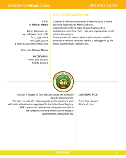
ECASA Study Site Report
Chioggia, Northern Adriatic Sea
Italy
ECASA partners:
14 - University of Venice
11- ICRAM
(Istituto Centrale per la Ricerca scientifica e
tecnologica Applicata al Mare - Chioggia
branch)
Roberto Pastres, Fabio Pranovi, Daniele Brigolin, Federico
Rampazzo,
University of Venice
Michele Giani, Otello Giovanardi, Fabio Savelli
Daniela Berto, Gianluca Franceschini
ICRAM
Version 3
1
This Study Site Report presents the results of the field surveys and of the model
applications aimed at testing the indicator and models at a an off-shore mussel farm.
The farm, Vi.S.Ma società cooperativa, was established in 1991. It is located
approximately 3 miles off-shore the city of Chioggia, on the Eastern coast of the
Northern Adriatic Sea, Italy. The Mediterranean mussel Mytilus galloprovincialis is
the only specie farmed, using a long-line system. The licensed surface covers an area
of about 4 Km2. Mussel farming is becoming an important complementary activity for
fishermen in Northern Adriatic, where fishery industry is suffering the consequences
of stocks decline. At present, the three Northern Adriatic Italian regions account for a
yearly production of about 30,000 x 103 kg, with about 500 people permanently
employed in this activity. With a current production of 600 x 103 kg year- 1, ViSMa a
farm can be regarded as a “typical” mussel farm in this region.
A comprehensive set of data was collected, in order to investigate the potential
impact of the mussel farm on both the pelagic and benthic ecosystems. Furthermore,
water quality parameters and on-growing mussel biometric parameters were
monitored during a typical rearing cycle, in order to relate mussel production to water
temperature and food particle availability.
The results indicate that off-shore long-line mussel farming can be managed in
a sustainable way along the North Western Adriatic coastline. The monitoring of the
on-growing mussel biometric parameters confirms that the ecosystem provides
sufficient resources for sustaining the mussel growth, which makes mussel farming a
profitable activity. Furthermore, the model MG-IBM successfully simulates the
mussel growth at this site and, therefore, allow one to predict the biomass yield as a
function of water temperature, Particulate Organic Carbon and Chlorophyll a
concentration.
As far as the potentially adverse effects are concerned, the assimilative
capacity of this area seems to be large, in relation to the pressure caused by the
presence of a typical mussel farm. In fact, no statistically significant difference was
found among the mean values of the water quality indicators at the reference stations
and at the two potentially impacted ones. The statistical analysis of the sediment
geochemistry data evidenced a moderate impact of the mussel farm on chemical
parameters. Both field data and a model simulation based on purposely modified
version of the particle tracking model MERAMOD indicate that this impact is
restricted to the sediment beneath the farm and the immediate surrounding. However,
this impact does not seem to severely damage the macrobenthic and meio benthic
communities, since the abundance and composition of the meiofauna are quite similar
at the reference and impacted stations, which are classify as “good” according to the
AMBI index.
These findings indicate that, as far as the ecological carrying capacity is
concerned, there is a potential for further expansion of this activity in this area.
However, such an expansion should be carefully planned, in order not to exceed the
carrying capacity of a given coastal area. To this regard, the model MCCC, tested
within this project, may represent valuable tools for planning the release of new
concession, in a Integrated Coastal Zone Management, ICZM, framework.
2
Contents
1. Introduction to the aquaculture operation ..................................................................4
1.1 Introductory background statement .........................................................................4
1.2 Summary statement of key site specific environmental issues ................................6
1.3 Information of farmer’s environmental strategy:.....................................................7
2. Site specific regulatory and management background ..............................................7
2.1 The regulatory status of proposed location with respect to fish farming
developments. ................................................................................................................7
2.2 Site description.........................................................................................................8
2.3 Detailed description of the farm ..............................................................................9
2.4 Proposed management strategy: biomass, medicines, chemicals, cycle, feed inputs,
growth measurements. ...................................................................................................9
2.5 Physical farm logistics, including type of gear used (Cages, long lines, rafts…),
moorings, access, lighting and anti-predator measures. ................................................9
2.6 Production and Processing.....................................................................................10
3. Description of the site and quantification of effects on the environment – existing
information only, not collected by ECASA. ................................................................11
3.1 Land use, landscape and visual quality..................................................................11
3.2 Hydrography and water quality .............................................................................11
3.2 Bathymetry, geology and habitats..........................................................................14
3.3 Benthos and sediments...........................................................................................15
3.4 Marine mammals; seals, cetaceans, otters .............................................................16
3.5 Birds .......................................................................................................................16
3.6 Fisheries and wild fish populations........................................................................17
3.7 Noise ......................................................................................................................17
3.8 Transport ................................................................................................................17
3.9 Socio-economic impact..........................................................................................17
4 Results of ECASA field studies: Indicators and Models applied and evaluated. .....18
4.1 Background to field programme: dates, staff, boats, stations sampled, etc. .........18
4.2 Sampling methods and materials, analytical methods. (Refer to the book of
protocols for detailed methods) ...................................................................................20
4.3 Models used and their parameterization. ...............................................................21
4.4 Results....................................................................................................................23
4.5 Evaluation of Indicator Performance .....................................................................36
4.6 Evaluation of Model Performance .........................................................................38
4.7 Site specific conclusions ........................................................................................40
4.8 Culture type and environment type conclusions....................................................40
5. Acknowledgements..................................................................................................41
6. References................................................................................................................41
Appendix 1. Details of all methods used (indicators, models, etc)..............................44
Appendix 2. Environmental data. ................................................................................45
Appendix 3. Models and their output ..........................................................................46
3
1. Introduction to the aquaculture operation
1.1 Introductory background statement
The Company.
Vi.S.Ma società cooperativa was established in 1991. Vi.S.Ma employs 9 people. In
1993, the company was given the license to farm bivalves in an area off-shore the city
of Chioggia, Northern Adriatic. The Mediterranean mussel Mytilus galloprovincialis
is the only specie farmed at the Chioggia site. The current production of the farm is
approximately 600 x 103 kg year-1.
• ECASA contributors:
DCF-UNIVE, ICRAM-Chioggia branch, HAIFA University
• Information sources – dates of site visits, other major sources:
The first survey was carried out the 16 December 2005. Eight field campaigns
were carried out, on a fairly regular basis, from July 2006 to May 2007
• who has been consulted and how:
Giuliano and Andrea Gianni (farm owners) have been the major source of
information, both when conducting site visits and when phoning for
information.
• difficulties encountered: high variability of the hydrological parameters and
sediment textures of the area, due to the influence of multiple riverine inputs.
Field Campaigns
The field work included two activities: 1) two pre-surveys and the main ECASA field
campaign; 2) the determination of time series of water quality and on-growing mussel
biometric parameters.
1) Pre-surveys and ECASA main campaign
ECASA contributors: DCF-UNIVE, ICRAM-Chioggia branch, HAIFA.
The ECASA campaign was carried in July 2006. It was preceded by two pre-surveys,
which are described in section 3.3, aimed at characterizing the sediment texture in the
area.
The following field deployments were made:
macrobenthos collection
meiobenthos collection
sediment collection
pH, Eh, dissolved oxygen and temperature at the sediment-water interface
redox potential in sediment core
CTD profiles (temperature, salinity, dissolved oxygen, chlorophyll, pH)
Secchi disc
Niskin bottles samples for nutrients and particulate matter analyses.
A current-meter was deployed from July to September 2006 and from April to
May 2007.
The following laboratory based analysis were carried out:
Sediment:
Granulometry
Water content
4
Loss On Ignition (LOI) 250°C e 450°C
Total Carbon
Inorganic Carbon
Total Nitrogen
Total Phosphorus
Inorganic Phosphorus
137
Cs and 210Pb in sediment cores
Water:
Particulate Organic Carbon
Particulate Total Nitrogen
Suspended Matter
Particulate Organic Matter
Particulate Phosphorus
Chlorophyll a
Ammonium
Nitrate
Nitrite
Silicates
Total Dissolved Phoshphorus
Total Dissolved Nitrogen
Phosphate (SRP)
Dissolved Organic Carbon
2) Time series of water quality and on-growing mussel biometric parameters
ECASA contributors: DCF-UNIVE, ICRAM-Chioggia branch.
Water quality and mussel biometric parameters were collected during the typical
rearing cycle of the Mediterranean mussel in this area. This activity was aimed at
calibrating the Mytilus galloprovincialis individual based model previously
identified by DCF_UNIVE, on the basis of literature data. Eight field campaigns
were carried, on a fairly regular basis, from July 2006 to May 2007.
The following samplings were made:
mussel specimen from the same rope
water by Niskin bottles sampling
The following measurements were made:
CTD collection (temperature, salinity, dissolved oxygen, chlorophyll, pH)
Secchi disc
The following laboratory based analysis were carried out:
Water:
Particulate Organic Carbon
Particulate Total Nitrogen
Suspended Matter
Particulate Organic Matter
Particulate Phosphorus
Chlorophyll a
5
Ammonium
Nitrate
Nitrite
Silicates
Total Dissolved Phosphorus
Total Dissolved Nitrogen
Phosphate (SRP)
Dissolved Organic Carbon
Mussel shell:
Length
Width
Thickness
Shell weight
Mussel soft tissue:
Wet weight
Dry weight
Ash Free Dry Weight
The procedures used for field measurements and laboratory analysis are described in
detail in the book of protocols and, whenever different, in Section 4.
1.2 Summary statement of key site specific environmental issues
The ViSMa mussel farm is located in the Northern Adriatic, near the city of Chioggia,
in the Regione (county) Veneto coastal area, Italy. The farm is located approximately
3 miles off-shore. As far as sediment texture is concerned, the study area lies in a zone
of transition between a belt of pelite and one of sandy pelite. With respect to natural
amenities, the seabed not far from the area is characterized by the presence of the
“Tegnue”, which are rocky aggregations emerging from the sea bed
(http://www.tegnue.it). In general, the water quality in the area is good with levels of
dissolved oxygen often close to saturation in the superficial waters. The area can be
affected by the discharges of the rivers Brenta, Adige and, to a lesser extent, Po. The
extent of the riverine influence depends on the season and winds.
From a socio-economic perspective, shipping, gas extraction, tourism,
professionale and recreational fishery are the main activities which can generate
conflicts with mussel farming. Infact:
1. the area is crossed by important commercial ship routes;
2. gas platforms are found in this area;
3. the marine protected area named “Tegnue di Chioggia” is located along the
coastline;
4. professional fishery, including beam-trawl fishery and Chamelea galina
fishery is commonly practised in the area;
5. recreational fishery is widely diffused.
The main use conflict arises between clam fishers and mussel farmers for the use
of the coastal zone, since clam fishery is not possible in the areas licensed to mussel
farming. This may represent a constraint to the further expansion of this actvity,
which is becoming an important complementary activity for fishermen in Northern
Adriatic
6
1.3 Information of farmer’s environmental strategy:
ViSMa has no documented environmental strategy, within ISO14001 standards.
Current regulatory status
The farming area was licensed to ViSMa by the “Genio Civile” of Rovigo, a local
authority which is entrusted the concession of farming areas, on behalf of Veneto
county (Regione Veneto).
2. Site specific regulatory and management background
2.1 The regulatory status of proposed location with respect to fish farming
developments.
Visma farm is part of the Veneto OP (Organizazione dei Produttori), a consortium
among producers which, in accordance with CEE 3759/92 directive, is aimed at
regulating the market supply and guarantee a quality standard for the product.
The current regulatory status in Italy entrusts the granting of licenses for marine
mussel culture sites to each county, Regione. This means that the regulations may be
different from place to place. The Northern Adriatic Italian coastline is under the
control of three “regioni”, namely, from North to South: Friuli Venezia Giulia, Veneto
and Emilia-Romagna. The latter is striving to frame the granting of shellfish licences
in a ICZM approach, in order to conciliate different coastal uses. On the contrary,
Veneto, at present, has no ICZM master plan. Therefore, each license request is dealt
with individually, and the decision is based on a technical consultation involving 11
different agencies, namely:
•
Capitaneria di Porto del distretto marittimo di competenza;
•
Agenzia del demanio;
•
Comune di competenza;
•
Ministero delle comunicazioni, direzione generale per le concessioni e
autorizzazioni;
•
CNR - Istituto di scienze marine ISMAR Sezione pesca marittima;
•
ICRAM – Istituto Centrale per la Ricerca scientifica e tecnologica Applicata al
Mare;
•
Ministero delle attività produttive ufficio nazionale e minerario idrocarburi e
geotermia;
•
Azienda U.L.S.S. dipartimento di prevenzione servizio veterinario del distretto
di competenza;
•
Comando in capo del dipartimento militare marittimo dell’Adriatico;
•
Istituto idrografico della marina militare;
7
•
Marina militare – Zona dei fari e segnalamenti marittimi;
With respect to food safety (Decr. Leg.vo 530/92 which accomplish 91/492/CEE
directive), Visma farm is located in waters classified as ‘zone A’, which means that
the reared mussels does not need a depuration period and can be marketed directly
after being harvested.
2.2 Site description
ViSMa farm is located in the Northern Adriatic Sea, south to the city of Chioggia. The
distance from the coastline is approximately 3 miles, see Fig. 1. The area is rather
shallow: depth ranges from 20 to 24 m.
Brenta
Adige
Western Adriatic coastal current
Study site
Po
Figure 1. Map of the area.
Along the north-eastern Adriatic coast the circulation is characterized by the
southward flow of the North Adriatic Current which exhibits a seasonal weakening in
the summer period, related to the stratification of the water column (Cushman-Roisin
et al., 2001). The thermoclyne disappears in winter, when the current transports well
mixed low-temperature and low-salinity waters. As a consequence, the area is mainly
influenced by the runoff of the rivers Adige, Brenta-Bacchiglione. The plume of the
river Po can reach the area in summer time or when the local circulation is driven by
strong southern winds. From the sedimentological point of view, the mussel farm is
located in a belt of pelite and sandy-pelite which runs parallel to the coastline
(Brambati et al., 1983). No submerged aquatic vegetation can be found, due to the
high turbidity, in the vicinity of the farm. According to (Cornello et al., 2005), the
macrobenthic community in the area is dominated by the bivalve mollusc Corbula
gibba, the amphipod crustacean Amphelisca diadema and the errant polichaetes
Lumbrineris gracilis.
8
2.3 Detailed description of the farm
The ViSMa mussel farm was established in 1991, the average annual production is
about 600 MT (6x105Kg). At present the company counts 9 employees. Two members
of the staff are based at the company storehouse, in Chioggia, and take care of the
administration and management. The other seven employees work on a daily basis at
the farm site. The working vessel is provided with toilet, showers and a kitchen,
allowing the employees to work for the whole day at the site. The farm is reachable in
approximately one hour time from the Chioggia harbor, therefore there is no need for
the employees to sleep on the boat. The company owns two vessels: one is used to
collect and process the product on site, while the other one is a carrier, used for
reaching the harbor. In this way, the product can be landed for distribution several
times during the same working day, without interrupting the recollection and
processing work. Historical current meter data indicate that the principal current
direction is south east, with an average module of 6 cm sec-1 near the bottom. This
pattern is more marked in winter time.
2.4 Proposed management strategy: biomass, medicines, chemicals, cycle, feed
inputs, growth measurements.
The mussel on-growing cycle lasts 10 to 12 months. Mussels are harvested starting
from late spring, but the most relevant fraction of the production is harvested in June,
July and August, when the demand is higher.
2.5 Physical farm logistics, including type of gear used (Cages, long lines,
rafts…), moorings, access, lighting and anti-predator measures.
The licensed area covers a total surface of 4 Km2, of which 3 Km2 were cultured in
2006-07. Mussel are reared using 1000m long lines, on which mussel nets are
suspended. The distance among lines is roughly 40 m, see Fig. 2a,b. Overall, the total
length of lines is 38 km. The average distance between suspended mussel ropes is of
0.7m and the average length of a rope is 2m. Ropes are suspended at a depth which
ranges from 3m to 7m.
9
40m
c
40m
3m
7m
c
2m
c
0.7m
Figure 2a,b. a) Schematic representation of mussel suspended culture at ViSMa farm; b) detailed
picture showing a mussel line and the suspended ropes.
2.6 Production and Processing
Mussel are collected and processed on board of the ViSMa vessel (Fig.3). Specimen
are sorted according to their size by means of a mechanical device. Marketable
specimen are cleaned and packaged, since the farm is located in an area classified as
‘zone A’ in regard to shellfish culture and fishery, which means that mussels do not
need to be treated at a depuration centre.
Figure 3. Vessel used for mussel husbandry.
10
3. Description of the site and quantification of effects on the environment –
existing information only, not collected by ECASA.
3.1 Land use, landscape and visual quality.
ViSMa farm, Fig. 4., is located off-shore the city of Chioggia, which population is
approximately 50.000 inhabitants. The city has a tradition as a fishing port and it is
one of the major fish marketplace in Italy. Tourism has recently increased its
importance. The coastal area in front of Chioggia is crossed by several commercial
ship routes and is used for trawl fishery and mussel farming. With respect to natural
amenities, the seabed in the North Western Adriatic coastal zone is characterized by
the presence of rocky aggregations emerging from the seabed, which are called
“Tegnue” (http://www.tegnue.it). Such aggregations can also be found in the vicinity
of the Visma mussel farm. This peculiar environment has been recently investigated
in
the
framework
of
the
INTERREG
III
project
(http://www.arpa.veneto.it/home/htm/interreg.asp), since it is characterized by high
biodiversity. The “Tegnue” Marine Protected Area was instituted with D.L. 5 August
2002. Different recreational sites are located along the coast, between Chioggia and
the Po Delta, including the towns of Sottomarina, Rosolina and Albarella.
Figure 4. View of the farmed area.
3.2 Hydrography and water quality
The area can be affected by the discharges of the rivers Brenta, Adige and, to a lesser
extent, Po (see Fig. 1). The extent of the riverine influence depends on the season and
winds. The plumes of Brenta and Adige are more likely to reach the study area in
autumn and winter time, when the circulation is driven by the Western Adriatic
Coastal current. The mean daily discharges of the river Adige and Brenta, including
its tributary Bacchiglione, were about 155 m3 s-1. and 76 m3 s-1 in the years 2004-05.
The mean daily discharge of the river Po, the largest Italian river, in the years 20022006 was 1157 m3 s-1.The central and northern distributaries of the Po delta, Po di
Maistra and Po della Pila, account for at least 70% of the total discharge and, can
influence the study area in spring and summer time, when southerly winds blow.
11
Large inter-annual variations of temperature and salinity are typical of the
Northern Adriatic Sea. As one can see from Fig. 5, the water column is stratified in
spring and summer. Water temperature ranges from in 25-26 °C (surface) and 20-21
°C (bottom) in August, to 5-6°C (surface) and 7-8 °C (bottom) in February-March.
0
St. BA
profondità (m)
-5
-10
-15
-20
-25
L A S ON D G F MA M G L A S O N DG F M A M G L A S O N D G F M A M G L A S
1999
2000
2001
2002
0
St. BA
profondità (m)
-5
-10
-15
-20
-25
L A S ON D G F MA M G L A S O N D G F M A M G L A S ON D G FM A M G L A S
1999
2000
2001
2002
Figure 5. Monthly variations of temperature and salinity profiles at a sampling site at the north-west
edge of the mussel farm (from Giovanardi et al., 2003).
Time series of current velocity were collected in 2001-2002 at site G, see Fig.
9, within the mussel farm. The current-meter was placed two meters above the seabed.
The descriptive statistics, which are summarized in Table 1, show that the main
current is oriented towards south-east and the average velocity is 6 cm sec-1. The
progressive vector diagram for a winter and summer period are shown in Fig. 6. The
main current direction is south east and more marked in winter time than in summer
time, when the Western Adriatic Coastal current is weaker. However, the dispersion
around the mean is rather high (CV% = 79%), because of the systematic variations
induced by the tide.
Table 1. Descriptive statistic concerning the current velocity data. The current-meter was placed two
meters above the seabed.
Current velocity module Current velocity direction
[cm sec-1]
[degrees with respect to north]
Valid N
31310
31310
Mean
5.7
181.5
Median
4.9
163.5
Minimum
0
0
Maximum
62.1
359.7
Std.Dev.
4.5
93.3
12
Figure 6. Progressive vector diagram in winter time, 19/12/2001-18/2/2002 (left), and summer time,
11/7/2002-17/8/2002 (right).
In general, the water quality in the area is good. The results of a 3 years long
survey, (Giovanardi et al, 2003) show that, in the years 1999-2002, DO was often
close to saturation in the superficial waters at site BA, within the mussel farm.
However, values as low as 50% were recorded in summertime near the seabed.
The seasonal evolution of several water quality parameter was determined at
site S2 located about 2 km NW, see Fig. 8, in the years 1995-96 (Giani et al., 2000,
Catalano et. al., 1996). The average POC concentration was 25.6 ± 15.1 µmol L-1 , PN
3.8 ± 2.2, TPP 0.19 ± 0.12, and Chlorophyll a ranged from 0.4 to 16 µg L-1. Due to
the influence of the rivers and sediment resuspension, the turbidity is rather high: the
average Secchi Disc was 3.7m.
Giani et al. (2000) studied the vertical distributions and temporal variability of
Particulate organic C, N and P at station S2. Particulate Organic Matter distribution in
superficial waters is highly variable, reflecting the allochthonous inputs coming from
the rivers. The inverse correlation found by these authors between POC, TPN, TPP
and water Salinity, indicates the importance of river discharges as sources of
suspended particulate matter. Similarly, peaks in dissolved nutrient concentrations,
which sustain the primary productivity, are associated with river discharges. TPP
concentrations in superficial waters, ranging between 0.15 and 0.22 µmol L-1, exceeds
of approximately one order of magnitude the ones measured by the same authors at a
station located in the central Northern Adriatic. The C:N:P ratios reported by Giani et
al. (2000) for low salinity superficial waters are close to the Redfield’s ratio
(107.7:16.3:1), suggesting that phytoplankton represents an important component of
the suspended matter. As regards high salinity deep waters, the reported C:N:P ratio is
of 69.5:8.1:1; this increase in N and P concentrations can be related to events of
sediment resuspension. As far as phytoplankton community composition is concerned,
Bernardy-Aubry et al. (2004) studied the succession of algal species in the NorthWestern Adriatic coast during a 10 year sampling period (1990-1999). According to
these authors, the dominant species in late-winter (February) is Skeletonema costatum.
During spring the community is dominated by diatoms, while the algal biomass in
summer is mostly accounted for flagellates. The late summer peak is characterized by
the presence of large diatoms, with a high carbon content.
Brigolin et al. (2006) estimated in approximately 5 hours the flushing rate for the
ViSMa farm. This calculation was carried out by assuming the presence of a constant
13
current (5 cm s-1 module). This situation is typical of the winter time. For the summertime case, see the right-hand side of Fig. 6, the transit-time estimation should be
improved by taking into account the turbulent diffusion. This can be carried out by
means of advection-dispersion models (e.g. MERAMOD), or wider-scale
hydrodynamic models of the Adriatic Sea (different hydrodynamic models are
available for this area: e.g. MFSTEP, 2004; Janekovic and Kuzmic, 2005; Lovato et
al., 2007).
3.2 Bathymetry, geology and habitats.
The spatial distribution of sediment texture in the area is shown in Fig. 7. As one can
see, the study area lies in a transition area between a belt of pelite and one of sandy
pelite, which extend parallel to the coastline in the NW-SE direction (Brambati et al.,
1983). Fine sediments such as silt and clay are mainly supplied from the northern
Adriatic Sea rivers (Brambati et al., 1973) and they are distributed along the Italian
coast by the Western Adriatic Coastal current. Suspended sediments are mechanically
sorted out by their grain size: as a result, the sediment grain size decreases southward,
as the distance from river mouths increases from (Brambati, 1973, Wang and Pinardi,
2002).
Submerged aquatic vegetation is absent in the area, because of the rather high
turbidity.
Figure 7. Map of sedimentological texture of the North-West Adriatic Sea. (Brambati et al., 1983).
The red circle marks the position of the mussel farm.
14
3.3 Benthos and sediments
Data concerning the macrobenthic community were collected by ICRAM underneath
the VISMA cultivation site during a three year long research program (Jul 99- May
01). The averaged taxa composition is reported in Tab. 2. The dominant species are:
the bivalve mollusc Corbula gibba, the amphipod crustacean Amphelisca diadema
and the errant polichaetes Lumbrineris gracilis (Cornello et al., 2005).
Table 2. Macrobenthos taxa composition beneath the cultivation site.
taxa
BIVALVES
RELATIVE
ABUNDANCE %
24.1
GASTEROPODS
1.3
ERRANT POLICHAETES
28.4
SEDENTARY POLICHAETES
23.7
AMPHIPODS
10.3
DECAPODS
3.7
ECHINODERMS
6.6
OTHER
1.9
As reported in section 3.2, the study site is on the edge of the area influenced
by the rivers Adige, Brenta and Po. The deposition of riverine sediment, finer and
richer in Organic Carbon and Nitrogen in comparison to sand, may superimpose to the
effect of the deposition due to the presence of the mussel farm. Therefore, in order to
get a clearer picture of the sediment texture, two pre-surveys in the area surrounding
and including the mussel farm were carried out.
On December 21st 2005 surface sediment (0-1 cm) was sampled in 20 stations
in a 3 x 4 km area surrounding the farm. Ten surface sediment sample were taken in
the following pre-survey, carried out on July 13th 2006, which was focused on a
smaller area, more likely to be impacted by the mussel culture activities.
The results of the pre-surveys are summarized in Fig. 8: data are presented in
detail in Appendix 2. As one can see, pelite and water content increases from NE to
SW: this feature is probably due to the sedimentation of suspended matter of riverine
origin. The distribution of organic carbon, see Fig. 8c showed a similar pattern. It is
interesting to note that the spatial distribution of total phosphorus (TP) is different: as
one can see from Fig. 8d, its concentration is higher beneath the farm, suggesting that
TP could be a useful indicator of the impact of the mussel culture. Similar patter was
observed for organic phosphorus.
15
Water content (%)
Pelite (%)
58
90 45.13
45.13
54
80
50
45.12
Lat. N
60
50
45.12
46
Lat. N
70
42
38
40 45.11
45.11
34
30
30
20
26
45.10
45.10
10
12.44
12.45
12.46
12.47
22
0
12.48
12.44
12.45
Long. E
12.46
12.47
18
12.48
B)
Long. E
A)
Total phosphorus (mg/kg d.wt.)
Organic carbon (% d.wt.)
620
1.8
45.13
600
45.13
580
1.6
560
540
1.4
Lat. N
1.2
1
520
45.12
500
Lat. N
45.12
480
460
440
420
0.8 45.11
45.11
400
380
0.6
360
340
0.4
320
45.10
45.10
300
0.2
280
12.44
12.45
12.46
Long. E
12.47
0
12.48
C)
12.44
12.45
12.46
Long. E
12.47
12.48
260
D)
Figure 8. Distribution of pelite (A), water content (B), organic carbon (C) and total phosphorus (D) in
surficial sediments. The poligon represent the area of the mussel farm. The triangles indicate the
sampling sites.
3.4 Marine mammals; seals, cetaceans, otters
The presence of Dolphins and Sea Turtles was observed nearby the farm (Visma
farmers, pers. comm.).
3.5 Birds
There is no evidence that the current aquaculture activities at ViSMa Site may have an
impact on the migratory bird populations.
16
3.6 Fisheries and wild fish populations.
According to 2003-2004 data (http://www.adrifish.org), the major captures in the
Chioggia area are Anchovies, Sardines, Cuttlefish, Sole, Mantis Squillid. One of the
gear used is ‘rapido’, a beam-trawl for soles and scallops employed in the Northern
Adriatic sea. A relatively high level of disturbance of this gear on benthic
communities was assessed by Pranovi et al. (1998) for a study site located in this area.
To this regard, the presence of a mussel farm may have a positive impact on the
sediment underneath, preventing from the rapido boat transit.
Clam (Chamelea gallina) fishery is also an important activity within the first
three miles from the coast. Since clam fishery is not possible in the areas licensed to
mussel farmer, there is a conflict between clam fishers and mussel framers for the use
of the coastal zone. For this reason, the concession of a mussel culture area is
subjected to the permission of a regional committee, which involves stakeholders
from both mussel culture and clam fishery sectors.
3.7 Noise
Given the distance from the coastline, no evidence of problems to noise have been
reported.
3.8 Transport
The site can be accessed by boat. ViSMa company fishing boat visits the site on a
daily basis.
3.9 Socio-economic impact
Visma can be regarded as a medium size farm in the Veneto area. However, according
to Prioli (2006), mussel farming is becoming an important complementary activity for
fishermen in Northern Adriatic, where fishery industry is suffering the consequences
of stocks decline. As one can see from Table 3, at present, the three northern adriatic
italian regions account for a yearly production of about 30,000 MT, with about 500
people permanently employed in this activity. This figure, which almost certainly
underestimate the man power involved in mussel farming, is expected to increase,
since the demand for new licensed area is still very high.
Table 3. Socio-economic data regarding shellfish culture in the Northern Adriatic Sea
N° of
Long-lines
Production
County
farms
length (m)
Species
(MT)
Friuli Venezia
Giulia
Veneto
EmiliaRomagna
N°
employed
19
18
165640
415000
M.galloprovincialis
M.galloprovincialis
3624
10572
60
150
23
583143
M.galloprovincialis
16639
250
17
4 Results of ECASA field studies: Indicators and Models applied and evaluated.
4.1 Background to field programme: dates, staff, boats, stations sampled, etc.
As mentioned in section 1.1, the field work included two main activities: 1) the main
ECASA field campaign; 2) water quality and on-growing mussel monitoring. For the
sake of clarity, these activities are separately described in the two following subsections.
1) ECASA field campaign
The main field campaign was carried out on July 13th, 18th and 25th 2006 and was
aimed at the assessing the adequacy of indicators, identified by WP2 and WP3, and
models, proposed by WP4, for EIA of off-shore long-line mussel farm. An adequately
equipped fishing boat made available by ViSMa was used for the sampling activities,
which were carried out by ICRAM personell (Michele Giani, Daniela Berto, Fabio
Savelli) and DCF_UNIVE personell, temporarily employed to work on the ECASA
project (Federico Rampazzo and Daniele Brigolin). Bioessays were deployed with the
help of Dror Angel, Haifa University.
The sampling stations were chosen on the basis of the data collected in two
pre-surveys, see section 3.3, and of a time series of available sites-specific
hydrographic data, see section 3.1. Sampling sites are displayed in Fig. 9: their
geographical coordinates are included in the data set, as detailed in the appendix.
Sediment, meiofauna and macrofauna samples were taken at sites B, D and G.
Sediment cores were taken using a box-corer. The site for sediment sampling were
selected in the oldest area of the farm, along the prevailing direction of the current.
Site B, upstream the main current, was selected on the basis of the results of the
presurvey, which indicates that the sediment texture markedly changes if one moves
further to the north. In fact, sediment texture in the area changes abruptly due to the
effect of the river plumes, as can be seen in Fig. 8a. The list of sediment parameters
determined either is situ or in subsequent laboratory analysis is presented in section
1.1.Two radioactive isotopes, 137Cs and 210Pb, were measured in the sediment core
sampled at sites D.
Water was sampled at sites A, E and G, at three depths, namely at the surface,
at 10 m and 20 m. The list of water quality parameters determined either in situ or in
subsequent laboratory analysis is presented in section 1.1.
Bioassays experiments were carried out in collaboration with D. Angel,
HAIFA University, at sites S2, G, H, L, in order to assess the potential for
phytoplankton growth in the area. Four dialysis bag were placed at two depths, (1.5
and 6 m) on July 20th and collected on July 25th. The following parameters were
measured “in situ” using a CTD probe: water temperature, salinity, pH, turbidity.
POC, phosphorus and chlorophyll a concentrations in seawater collected from each
bag at the end of experiment. Chlorophyll-a analysis were carried out by ICRAMRoma.
A complementary time series of hydrographic parameters was collected in
2006-2007. A current-meter was deployed at site C at a depth of 6 meters by ICRAM
personnel (Gianluca Franceschini) from July to September 2006 and from April to
May 2007.
18
Figure 9. Sediment and water sampling stations in the ECASA main field campaign. Red squares
represent the boundaries of mussel lines.
19
2) Time series of water quality and biometric parameters of on-growing mussel
This activity was aimed at testing the models proposed by WP4 for site selection and
EIA of off-shore long-line mussel farm. Water quality parameters were determined at
the three stations A, E, G in Fig. 9, located along a NW-SE transect. Eight field
campaigns were carried, on: Jul-13-2006, Aug-17-2006, Sep-4-2006, Nov-11-2006,
Dec-19-2006, Jan-30-2007, Apr-3-2007, May-22-2007.The sampling activities were
operated by ICRAM personell (Michele Giani, Daniela Berto, Fabio Savelli) and
DCF_UNIVE personell, temporarily employed to work on the ECASA project
(Federico Rampazzo and Daniele Brigolin).
Water temperature, salinity dissolved oxygen, fluorescence and turbidity
profiles were determined in situ using a CTD probe. The following indicators were
determined on water samples: dissolved organic carbon, particulate organic carbon,
particular total nitrogen, suspended matter and POM, particulate phosphorus,
chlorophyll-a, ammonium, nitrate, nitrite, silicates, Phosphate (SRP), TDP, TDN.
Mussel specimen were collected at site N, see Fig. 9, and the following
biometric parameters were subsequently determined: wet weight, dry weight, shell
length, width, thickness and weight, AFWD. Two condition indexes were determined,
namely dry weight/shell weight (DW/SW) and ash free dry weight/shell weight
(AFDW/SW). Based on the findings presented in (Boscolo et al., 2002), these indexes
are the most sensitive to the physiological and nutritional mussel condition. Mussel
were not sampled on August 17 2006.
4.2 Sampling methods and materials, analytical methods. (Refer to the book of
protocols for detailed methods)
Sediment. Sediment samples were collected using a box-corer. Three replicates were
taken at each sampling site. Sediment cores were pre-treated according to the book of
protocols. The first top 12 cm were sliced, in order to determine the vertical profiles
of the variables listed in section 1.1.
Sedimentation rate were calculated from 137Cs and from the CF-CM model applied to
210
Pb profile. 137Cs was counted via gamma spectrometry using coaxial intrinsic
germanium detector (Frignani et al., 1993). 210Pb activities was determined through
the measurements of its daughter nuclide 210Po using a alpha spectrometry (Frignani
and Langone 1991, Frignani et al., 1993).
Macrofauna. Macrofauna was sampled using a box corer.
Meiofauna. Meiofauna was sampled using a box corer.
Water. Water samples were collected using Niskin bottles. Bioassays were carried
out in agreement with the book of protocols. Laboratory analysis were carried out in
accordance with the book of protocols except for Total particulated Phosphorous was
determined spectrophotometrically using the molibdic blue method (Murphy & Riley
1962). The filtration was carried out according to the book of protocols for particulate
matter. Filters was combusted at 550°C for 4 hours. Phosphorous was extracted using
1 N HCl, sonicating for 15’. Subsequently the extraction was conduced for 16 hours
under agitation modified from Aspila et al. (1978 ). KH2PO4 standards were used for
the calibration curve. Detection limit was 0.1umol P L-1.
20
4.3 Models used and their parameterization.
MERAMOD
One of the goals of the field program was to test the applicability of the particle
tracking model MERAMOD (http://meramed.akvaplan.com) to site selection and EIA
of long-line mussel farms. MERAMOD is a well-developed deposition/impact model,
designed for fish cages and routinely used by SEPA for site selection, EIA and
monitoring guidelines recommendation (Cromey et al., 2002a,b). The program was
modified, in close collaboration with SAMS, in order to enable the simulation of the
dispersion and sedimentation of bio-deposits released by a long-line mussel farm.
Each line is modelled as a point-source of suspended organic matter, namley mussel
faeces and pseudo-faeces. The faeces production rate per mussel line, f, was estimated
according to the formulation:
f = POC ⋅ CR ⋅ n ⋅ DW ⋅ ( 1 − AE )
(1)
where: POC represents the yearly averaged Particulate Organic Carbon concentration
in the area, CR is the Clearance rate of the mussel, n represents the number of
individuals per line of farm, DW is the average weight of the mussel and AE is its
Adsorption Efficiency. The parameters n and DW were estimated on the basis of
husbandry information and CR and AE on the basis of data concerning the physiology
of M. galloprovincialis.
MG-IBM, Mytilus Galloprovincialis Individual Based model
The model, which has been designed and identified during the ECASA project,
simulates the evolution of two state variables, namely the dry weight of somatic and
gonadic tissue.
The state equations read as:
dWb
A−C
= (1 − k ) ⋅
dt
εB
dR
A−C
=k⋅
εR
dt
(2)
where Wb represents the somatic dry weight of the mussel and R the gonadic dry
weight . The energy budget is computed as a difference between the daily anabolism,
A, and the daily catabolism of the mussel, C, both expressed in [J·day-1]. The
parameter k [adimensional] quantifies the fraction of energy transferred to the gonadic
compartment, while B and R are respectively the energy content of somatic and
gonadic tissue [J·gdW-1]. The model is described in detail in Brigolin (2007). All
model parameters, except for k, were estimated on the basis of literature information.
The fraction of energy allocated in reproduction was calibrated against the times
series of mussel biometric parameters collected at ViSMa site.
21
MGCC Mytilus Galloprovincialis Carrying Capacity model
The individual based model of MG-IBM is the core of an integrated model, which can
be used at two scales: at a farm scale, or scale A, for site-selection and EIA of longline mussel farm; at a regional scale, or scale C, for estimating the overall impact of
mussel farming on the pelagic ecosystem and the carrying capacity of a given area.
The scale C application needs to be supported by site-specific ecological and
hydrodynamic models. Within the ECASA project, a preliminary scale C application
at the Northern Adriatic coastline was attempted.
The model is made up of thee modules: a transport module, a biogeochemical
module, and the MG-IBM module. The transport model is based on a finite difference
TVD-MUSCL scheme (van Leer, 1997), adopting orthogonal or boundary fitted
coordinate system. This scheme has second order accuracy in space and is mass
conservative. This approach allows one to change the grid size within the
computational grid: this feature is essential for scale C applications, since the correct
simulation of the near-field perturbation due to the presence of the farm requires a
25m grid size, which is then increased up to 400m when modelling the transport and
biogeochemical processes among farms. The biogeochemical module is based on a
simplification of the ERSEMIII equations reported by Vichi (2002). It includes the
following state variables: concentrations of DOC, POC, nitrate, ammonia, reactive
phosphorous and silicates, densities of phytoplankton, zooplankton and mussels in
farming sites. Model equations are described in detail in Brigolin (2007).
Model parameters were estimated on the basis of the literature, except for the eddy
diffusivities, which were calibrated by comparing the model output with water quality
data at Chioggia site.
The model was then used for simulating the local impact of mussel farming on
chlorophyll-a and dissolved ammonia concentrations and for analysing the
consequences of an increase in the number of mussel farms in the area on water
quality and biomass yield.
22
4.4 Results.
Currents
The results are summarized in Tab. 4, which presents the main descriptive statistical
indexes.
Table 4. Descriptive statistic concerning the current data.
July-September 06
Valid N
Mean
Median
Minimum
Maximum
Std.Dev.
April-May 07
Valid N
Mean
Median
Minimum
Maximum
Std.Dev.
Current velocity
module [cm sec-1]
4032
12.56
11.24
0.00
54.76
7.86
Current velocity
module [cm sec-1]
2902
13.9
12.2
0.0
45.0
8.3
Current velocity direction [degrees with respect
to north]
4032
183.51
174.39
0.00
358.28
65.27
Current velocity direction [degrees with respect
to north]
2902
170.0
165.3
0.00
359.7
74.2
The main current was oriented towards south for the summer 2006 and southsouth-east for spring 2007. The mean velocity was slightly higher in the spring 2007.
similar. The standard deviations in both cases are rather high, because of the
systematic variations induced by the tide.
Water
The results concerning the water quality indicators presented in this section refers to
the time series collected at sites A, E and G. This data set, which includes the data
collected in July 2006 as a subset, provides reliable and robust indications about the
impact of the mussel farm.
In accordance with the general features of the area, thermal stratification and a
marked halocline in the upper 5-8 meters were observed during the summer months.
The winter 2006/2007 was unusually mild: as one can see from Fig. 10, the average
surface water temperature at the three sampling stations was ~3°C higher than that
recorded at site S2, located approximately 2 km from the mussel farm, over the years
2001-2005.
23
30
Mean 2001-2005 values
2006-2007 values
28
26
24
22
[°C]
20
18
16
14
12
10
8
6
4
Lug
Sep
Nov
Jan
Mar
May
Figure 10. Comparison between the evolution of surface water temperature in 2006-2007 at sites A,E
and G and the average evolution over the years 2001-2005 at site S2, located approximately 2 km from
the mussel farm.
The mean values and the sample standard deviation, SSD, of the water column
indicators at the three sampling sites and depths are compared in Table 5. Standard
deviations are, in general higher for surface samples at the three stations, since the
surface layer is the most affected by river discharges: such variability should be taken
into account when comparing the mean values. As it will be shown in Section 4.5, the
data presented in Tab. 5 do not univocally indicate a strong impact of the farm on the
water column indicators. As regards the surface layer, Station E, which is in the
middle of the farm, presented the lowest Chla and the highest phosphate, nitrate and
Total Particulate Nitrogen mean values. Nevertheless, these potential signs of impacts
are in contrast with the fact that St. E also showed the highest POC and the lowest
ammonia mean concentrations. The differences among the three stations become
smaller as the depth increases and they are not significant if the variability is taken
into account, see section 4.5.
24
Table 5. Comparison among the mean values and
indicators at the three monitoring sites.
PO4 NH3 NO2 NO3 TDP
(µ
µM) (µ
µM) (µ
µM) (µ
µM) (µ
µM)
0.21
Asup Mean 0.07 0.56 0.24 7.11
Std
0.05 0.35 0.19 5.82
0.09
0.23
Esup Mean 0.14 0.55 0.28 7.7
Std
0.21 0.47 0.41 13.5
0.24
0.21
Gsup Mean 0.09 0.91 0.29 7.1
Std
0.06 1.28 0.38 10.8
0.11
A10
E10
G10
A20
E20
G20
the standard deviations of the water quality
TDN
(µ
µM)
17.06
6.96
17.29
17.69
18.32
13.88
SiO2
(µ
µM)
6.74
5.06
7.24
10.62
6.75
10.68
Chla
(µ
µg/L)
4.8
3.23
1.9
1.63
2.85
5.43
DOC
(µ
µM)
196.78
75.61
194.86
81.50
174.51
55.01
POC TPN
(µ
µM) (µ
µM)
32.41 4.6
27.09 4.05
36.16 4.7
41.83 3.77
22.15 3.13
11.70 2.27
Mean
Std
Mean
Std
Mean
Std
0.05
0.03
0.06
0.03
0.07
0.04
0.73
0.74
0.28
0.28
0.56
0.34
0.12
0.10
0.19
0.31
0.15
0.21
1.52
1.46
1.94
1.64
1.58
1.03
0.17
0.08
0.17
0.09
0.19
0.12
10.81
3.28
11.72
3.50
12.28
6.63
2.51
1.27
3.38
1.43
2.7
1.42
0.74
0.45
0.81
0.34
0.83
0.54
167.30 12.61
53.93
5.5
150.88 15.13
63.45 8.01
160.77 12.10
73.57 5.39
1.56
0.74
2.07
1.79
1.57
0.72
Mean
Std
Mean
Std
Mean
Std
0.07
0.04
0.07
0.04
0.07
0.05
0.74
0.82
0.64
0.69
0.80
0.71
0.16
0.25
0.21
0.40
0.12
0.10
1.04
0.71
0.91
0.56
0.86
0.51
0.17
0.08
0.16
0.08
0.16
0.11
10.20
3.49
9.70
3.75
7.79
4.66
3.2
3.41
2.76
3.37
2.18
2.84
1.12
0.54
1.05
0.55
0.95
0.73
163.46
47.59
153.61
72.00
150.01
45.71
1.81
0.58
2.10
1.23
1.76
1.18
14.9
3.74
14.7
4.63
11.9
5.55
The results of the bioassays are summarized in Table 6, which presents the average
initial and concentrations of Chla, POC and PON at sampling sites S2, G, H and L at
the two depths of 1.5 and 6 m and their standard deviations.
Table 6. Initial and final values of the indicators measured in the bioessay.
Initial values
Depth = 1.5m
S21.5
G1.5
H1.5
L1.5
Depth = 6m
S26
G6
H6
L6
POC
(µM)
mean
39.4
Std
7.5
PN
(µM)
mean
4.6
Std
0.7
Chla
(µg/l)
mean
1.51
Std
0.11
57.29
60.29
50.89
54.41
6.65
23.33
7.34
4.34
8.01
8.48
8.81
9.11
1.55
3.18
2.02
0.75
3.38
4.56
3.43
5.98
0.93
2.16
1.82
2.45
60.98
46.88
47.66
43.53
30.52
15.17
19.89
7.28
9.28
7.85
7.52
6.68
5.34
2.01
2.37
0.90
3.38
5.71
4.64
5.58
0.93
2.40
1.73
1.49
Chla concentrations showed a marked increase at all stations, 2.2-4.4 times in five
days, with respect to the initial values. The increase was more relevant at 6 m depth
particularly, at L and G sites (3.8-4.4 times). The highest concentrations were
25
observed at site L, which is located at a distance of approximately 750 m from the
farm: this result does not suggest that the potential nutrient enrichment caused by the
farm is the main factor which stimulates the primary production in the area. Instead,
the fact that the production was higher at 6m both at sites G and H suggests that, in
this period, the production at the surface may have been inhibited by the excess of
incident light.
Sediment
Sediment was sampled at stations B, D and G. The first two stations are close to the
water quality station A and E, respectively. In general, sediment parameters showed
little variation with depth, probably due to the mixing induced by bioturbation.
Therefore, the average values of the three replicates are representative of the
conditions at the three sampling stations. The results are summarized in Tab. 7, which
shows the values of the indicators in the top 0.5 centimetres, their mean values and
their range.
Overall, the sediment parameters indicate that site D is different from the B
and G and that the differences are consistent with the impact of the shellfish farm. As
one can see from Tab. 7, site D presents the lowest values of EH and the highest mean
values of the other indicators: silt, LOI (250° and 450°), OC, TN and TP. pH, not
shown in the table, was roughly constant and did not show significant variations
among stations. Furthermore, at site D, EH was found to be negative even in the top
0.5 cm, while it was positive or slightly negative in the core B and G.
The higher content of total nitrogen TN and the higher Corg/Ntot ratio at site D
could be attributed to the different deposition rate and composition of organic matter,
and to the reducing conditions.
Table 7. Superficial sediment, average core parameters and range.
Water
Silt
(%)
(%)
EH
(mV)
OC
TN
TP
C/N
Porg
Pin
LOI
LOI
(mol/kg)
(mol/Kg)
(mol/kg)
(mol/mol)
(mg/kg)
(mg/kg)
450 °C
250 °C
(%)
(%)
B0-0.5
29
43.9
160.6
0.6
0.07
0.012
9.3
53.2
313.9
3.3
0.7
D0-0.5
36
56.6
-13.6
0.8
0.07
0.012
11.4
106.8
277.4
3.9
2.0
G0-05
26
28.3
5.5
0.5
0.05
0.012
11.0
43.8
332.4
2.6
0.6
Bmean
25
40.5
-122.1
0.7
0.06
0.012
11.6
71.7
313.9
2.8
0.9
Dmean
35
63.0
-136.3
0.8
0.07
0.014
13
140.1
290.9
5.4
2.0
Gmean
26
32.8
-133.5
0.6
0.05
0.012
11.7
78.4
304.5
2.9
0.7
Bmin
Bmax
21
29.7
-164.3
0.6
0.06
0.012
9.3
7.12
261.6
1.3
0.3
29
52.7
+160.6
0.8
0.07
0.013
14.1
155.6
368.7
4.3
2.3
Dmin
Dmax
30
37
38.0
78.4
-165.0
0.7
0.03
0.12
8.4
32.1
240.6
3.9
0.9
-13.6
0.9
0.18
0.18
15.0
472.9
341.7
6.8
4.0
Gmin
Gmax
21
5.9
-182.6
0.5
0.03
0.012
10.4
2.5
241.6
2.0
0.6
29
49.0
5.5
0.6
0.05
0.013
14.0
168.0
376.3
3.3
0.8
26
Radiometric dating analysis were performed in a core sampled at the D station in
order to assess the sedimentation rate in the mussel farming area. As one can see from
Fig. 11a and b, bioturbation is relevant in the surface layer, from 0 to 10 cm, where
the concentrations of radionuclides do not show marked gradients. From 210Pb and
137Cs profiles (Fig. 11) a sedimentation rate of 2-2.5 mm/years was estimated.
The average sedimentation rate was estimated by applying the Constant Flux –
Constant Sedimentation model to 210Pb profile. (Yeager et al., 2004). A
sedimentation rate of 2.2 cm/years was estimated from the results of the regression,
shown in Fig. 11c. This finding is confirmed by the vertical 137Cs profile, which is
characterized by a passing depth of 12.5 cm, corresponding to a time span of 50 years.
In fact, 137Cs was introduced in the environment in the fifties, with the nuclear test.
Highest emission intensity was reached in 1963.
10
20
0
0
10
15
20
25
30
50
0
2
4
6
8
10
12
14
16
2
100
150
0
Depth (cm)
5
Depth (cm)
depth (cm)
(Bq/kg)
5
Pbxs (Bq/kg)
0
D core
Cs (Bq/kg)
10
15
210
137
20
Pb-214
25
ln
D core
y = -0.1426x + 5.5322
3
R2 = 0.987
4
Pb-210
30
5
Figure 11. Vertical profiles of concentrations of 137Cs, (left), 210Pb and 214Pb, (centre), and
regression of log-transformed 210Pb, (right): the sedimentation rate was estimated from the slope.
Meiofauna
The results of the analysis of meiofauna abundance and composition are shown in
Tab. 8. Meiofauna abundance was quite similar beneath the mussel lines, site D, and
at a reference station downstream, site B. Both abundances were lower than those
found at a mussel farm in the Tyrrhenian Sea (Mirto et al. 2000). The spatial pattern
of the abundance was characterized by nematode assemblage ranging between 238.82
ind/cm2 at site D, which is located under the oldest part of the farm, and 493.64
ind/cm2 at station G, at a distance of 100m from the mussel lines. No significant
difference was recorded for both copepods and kinorynchs. The Nematode/Copepods
ratio appears to decrease with increasing distance from the impacted station: therefore
this quantity may be introduced as an indicator for monitoring the impact of mussel
farms. Overall, these findings do not evidence a significant perturbation of the
meiobenthic fauna due to the presence of the mussel farm. In particular, meiofauna
abundance and composition at site D, beneath the farm, are quite similar to those
found a site B, which can be regarded as a reference site.
Table 8. Meiofauna abundances at stations D, G and B.
Abundance (ind/cm2) B
Nematodes
Copepods
Copepod nauplii
Kinoryncha
N/C
Meiofauna metazoan
217.76
14.25
7.46
1.75
15.67
251.10
D
211.18
14.47
6.25
0.66
33.78
238.82
G
321.27
14.04
9.21
0.22
27.41
493.64
27
Macrofauna
The analysis allowed the detection of 47 macrobenthic taxa, belonging to 5 different
Phyla (Tab. 9). Univariate indices, such as specific richness, total abundance, and
Shannon index, showed higher values in the station G, located 100 m from the farm,
whereas the macrobenthic assemblage showed no significant differences among sites.
The application of AMBI highlights some differences among the stations, but all
values are assigned to the ‘slightly polluted’ category. Finally, by using the m-AMBI
method, the stations B and D are categorized as ‘good’, whereas the stations G and M
are classified as ‘high’.
All this suggests that, even if some differences among the stations are detectable, the
mussel farm has little impact on the macrobenthic community.
28
Table 9. Macrofauna abundance (ind/m2) and indices at stations B, D, G, and M; data reported as
average values of 4 replicates.
Phylum
Species
B
D
G
M
Sipunculida
Phascolosoma sp.
9.80
9.80
Mollusca
Abra ovata
9.80
9.80
9.80
Aporrhais pespelecani
9.80
Calyptraea chinensis
9.80
Capitella capitata
9.80
Corbula gibba
19.61
19.61
29.41
78.43
Dentalium dentalis
9.80
Euspira guillemini
9.80
Haminoea navicula
9.80
9.80
19.61
Hydrobiidae
9.80
Leiostraca subulata
58.82
9.80
9.80
Loripes lacteus
9.80
Nassarius sp.
9.80
Nucula nucleus
19.61
9.80
19.61
Pitar rudis
9.80
Sphenia binghami
9.80
19.61
9.80
Tellina distorta
19.61
9.80
Tellimya ferruginosa
39.22
39.22
9.80
58.82
Thracia papyracea
9.80
Turritella communis
9.80
Annelida
Ampharetidae
9.80
Drilonereis filum
9.80
Euclymene santanderensis
19.61
29.41
19.61
Glycera convoluta
19.61
Goniada emerita
9.80
Harmotoe sp.
19.61
9.80
Lubrinereis impatiens
98.04
107.84
166.67
19.61
Lysidice ninetta
9.80
Marphysa belli
9.80
Nematonereis unicornis
9.80
29.41
Nereidae
9.80
Onuphys eremita
9.80
19.61
19.61
Owenia fusiformis
9.80
9.80
Pectinaria auricoma
9.80
Phyllodocidae
19.61
9.80
29.41
Sabellidae
9.80
Syllidae
9.80
Terebellidae
19.61
Arthtropoda
Ampelisca sp.
19.61
137.25
39.22
Copepoda
19.61
Crangon crangon
9.80
Leucon mediterraneus
9.80
19.61
9.80
Leucothoe sp.
9.80
Macrura Natantia
9.80
Echinodermata Amphiura chiajei
88.24
68.63
58.82
Ophiothrix fragilis
39.22
Trachythyone elongata
9.80
Specific richness
19
13
30
21
Total abundance
480.39
313.73
774.51
450.98
Shannon index
2.54
2.16
2.85
2.73
AMBI
2.76
1.43
1.23
1.63
m-AMBI
good
good
high
high
29
Mussel
The time series of mussel length is presented in Fig. 13. As one cans see, mussel shell
length ranged from 3.92±0.40 cm, on July 13th 2006, to 7.06±0.81, on May 2007.
Mussels showed a significant increase(ANOVA test F6,694=84.84, p<0.001) in the
mean values of the shell length over time except for November and December 2006
samples (Tukey’s test, p>0.05, Fig. 12). To this regard, a significant decrease in the
length on January 2007, with respect to December 2006, was observed, which was
likely due to a sub-sampling error. The decrease in the growth rate which was
observed in the autumn months is consistent with previous data collected at the same
site, (Giovanardi & Boscolo, 2003) which showed that the increase in mussel length
was not significant from November 2001 to January 2002. This could be due to both
the reduced food availability and lower water temperature: relative low values of
Particulate Organic Carbon were observed at a depth of 10 m in November (10.63
M) and December (6.36 M), at station A, near the mussels sampling station.
mussel shell length
10
Length / cm
8
6
4
2
0
22
03
30
19
07
5
-0
4
-0
00
-2
00
-2
0
10
0
20
00
-2
2-
1-
1
-0
-1
-1
7
7
7
6
6
6
06
0
20
0
-2
9-
7
-0
-0
04
13
Time
13-Jul-06
*
4-Sep-06
***
***
7-Nov-06
***
***
ns
19-Dec-06
**
ns
***
***
30-Jan-07
***
***
***
***
***
3-Apr-07
***
***
***
***
***
ns
22-May-07
*: p<0.05, **: p<0.01, ***: p<0.001
Figure 12 – Temporal variations of the mussel shell length at ViSMa farm (mean values and standard
deviation are reported) and Tukey’s test for length values.
30
The box plot presented in Fig. 13 summarize the time series of the distribution of the
condition index DW/SW and AFDW/SW.
a)
0.6
Mean
Mean±DS
Range not-Outlier
0.5
DW/SW
0.4
0.3
0.2
22/05/07
03/04/07
30/01/07
19/12/06
07/11/06
04/09/06
0.0
13/07/06
0.1
Time
b)
0.50
Mean
Mean±DS
Range Not-Outlier
0.45
0.40
AFDW/SW
0.35
0.30
0.25
0.20
0.15
0.10
22/05/07
03/04/07
30/01/07
19/12/06
07/11/06
04/09/06
0.00
13/07/06
0.05
Time
a)
13-Jul-06
*
4-Sep-06
***
***
7-N ov-06
***
***
ns
19-D ec-06
**
ns
***
***
30-Jan-07
***
***
***
***
***
3-Apr-07
***
***
***
***
***
ns
22-M ay-07
b)
13-Jul-06
***
4-Sep-06
ns
***
7-N ov-06
ns
***
ns
19-D ec-06
***
***
***
***
30-Jan-07
ns
***
ns
ns
***
3-Apr-07
*: p<0.05, **: p<0.01, ***: p<0.001
Figure 13– Box plot of the temporal variations of the condition indexes: a) DW/SW and b)
AFDW/SW and Tukey’s test results.
DW/SW values ranged from 0.28 ± 0.1 (av ± s.d) on September 2006 to 0.11 ±
0.016 on November 2006, while AFDW/SW index ranged from 0.26 ± 0.1 on
September 2006 to 0.07 ± 0.01 on November 2006. The highest range of variation
was found for both the indexes in September. These values are similar to those found
in a previous study for the same mussel farm (Boscolo et al., 2002). Both DW/SW
and AFDW/SW observed in September 2006 and January 2007 were significantly
higher than in the other months: this finding is consistent with the reproductive cycle
in this area, since the increase in mussel soft tissue before the gamete emission usually
31
ns
***
***
*
***
*
22-M ay-07
takes place in autumn and in the late winter, (Boscolo et al, 2002; Giovanardi &
Boscolo; 2003). The increase of the indeces in September 2006 could also be related
with water chemical parameters. High nutrients, Chl-a and POC values were found in
the surficial waters, mostly due to high riverine inputs, that increased food
availability.
The data collected in this annual study confirm the seasonal pattern of the
mussel growth which was observed in a previous three-year long study (Boscolo et
al., 2002). This pattern is consistent with the seasonal evolution of water temperature
and food availability, as is shown by the application of the individual based model,
presented in section 4.4.6.
4.4.6 Model application
MERAMOD
The model was used for predicting the spatial distribution of the deposition rate of
organic carbon per unity surface, due to the presence of the mussel farm. Deposition
rates were not determined directly using sediment traps and, therefore, the model
could not be validated in relation to its application to long-line mussel farms.
However, there are indirect evidences that the model results are quite reasonable. In
fact, the order of magnitude of the deposition fluxes are consistent with estimates
found in the literature, as summarized in Tab. 10. The spatial distribution of the
deposition fluxes is shown in Fig. 14: as one can see, the most impacted area include
station E, where the sediment parameters were found to be perturbed by the presence
of the farm.
At a more quantitative level, the model was used for estimating the amount of
OC per unity area deposited during the lifetime of the farm at the sampling stations.
The fluxes thus obtained were used for computing the OC concentrations in the
superficial sediment at steady state, based on the following diagenetic equation:
∂C
=Φ − v ⋅C = 0
(3)
∂t
Based on the assumption that the OC behaves as a conservative tracer, it is
possible to use Eq. (3) for obtaining a crude estimation of the maximum increase in
the organic carbon concentration, due to the deposition of the flux of mussel faeces
and presudofaeces. The sedimentation rate, v=2.5 mm y-1, was estimated on the basis
of the 210Pb e di 137Cs vertical profile (CF-CS model) (see 4.4) which were used as
passive radioactive tracers. A sediment density of 2.5 g cm-3 was assumed..
The estimates thus obtained were compared with the deviations from the mean
of the OC concentrations in the top 1 cm which were determined during the
presurveys (see section 3). The results are shown in Fig. 16: as one can see, the
model predictions are in good accordance with the deviations observed at stations B,
C, H, I, which are located at the edges of the farm. However, the model seems to
overestimate the depositions at sites A, L and M, within the farm. This is consistent
with Eq. (3), since the degradation of organic carbon was not taken into account.
32
Table 10. Estimates of Oorganic Carbon fluxes originated by mussel farms.
~ 70 g C m-2 yr-1, (Hartstein et al., 2005 ), New Zealand.
~ 60 g C m-2 yr-1 (Aleffi et al. ,1999), Gulf of Trieste, Italy
~ 40 g C m-2 yr-1, ( Hatcher et al. ,1994), Canada
3500
3000
gC m-2 yr-1
A
B
34
32
30
28
26
24
22
20
18
16
14
12
10
8
6
0
C
D
2500
E
F
2000
G
H
1500
I
L
1000
M
500
500
1000
1500
2000
2500
3000
3500
Figure 14. Spatial distribution of the yearly depositions of organic carbon released by the mussel farm
predicted by a purposely modified version of MERAMOD.
0.8
OC [%]
0.6
0.4
obs
model
0.2
0
-0.2
A
B C D
E
F
G H
I
L
M
-0.4
.
Figure 15. Comparison between the observed concentrations of OC in the superficial sediment and
those estimated using MERAMOD.
33
MG-IBM
The model was successfully applied to the simulation of the growth of a cohort of
specimen, which were seeded in July 2006. The evolution of the forcing functions is
shown in Fig. 16a. The trajectory of the calibrated model is compared with the
observations in Fig. 16b. Only one parameter was calibrated, namely the fraction of
assimilated energy used for the production of gonadic tissue.
3.0
Environmental forcings Visma
POC [mg L-1]
chlorophyll-a [ug L-1]
water temperature [°C]
5.0
2.5
30
28
26
24
22
20
1.5
18
16
1.0
water T
POC, Chl-a
2.0
14
12
0.5
10
8
0.0
May-06
Jul-06
Aug-06
Oct-06
Nov-06
Jan-07
Mar-07
Apr-07
6
Jun-07
Figure 16a. Evolution of the forcing functions at the Chioggia study site.
1.6
1.4
mean Visma Ecasa field data
st.dev. Visma Ecasa field data
MG-IBM model
Dry weight [g]
1.2
1.0
0.8
0.6
0.4
0.2
0.0
May-06
Jul-06
Aug-06
Oct-06
Nov-06
Jan-07
Mar-07
Apr-07
Jun-07
Figure 16b. Model calibration: observed (dots) and predicted (continuos line) Mytilus galloprovincialis
dry weight.
34
MGCC
The results of this preliminary application of the integrated model are summarized in
Fig. 17a,b, which presents respectively the spatial distributions of Chlorophyll a,
(CHL), and ammonium (NH4) at steady state, and Fig. 18a,b,c, which shows the
average yearly concentrations of Chlorophyll a, ammonium and POC at the three
sampling stations.
The model correctly predicts a small impact of the farm on CHL concentration, which
is slightly depleted by mussel filtration, and POC, which is depleted by filtrations but
increased by biodepositions. As a result, POC is slightly higher within the farm, in
accordance with the indications provided by the time series of observations. However,
the model overestimates the increase in the ammonia concentration due to the release
of mussel excretion: field observations, in fact, show a slight decrease of ammonia
concentration within the farm.
9000
9000
1
0.95
2000
4500
0
2000
4500
0.95
4500
0.9
2000
0.85
2000
4500
[µΜ]
NH4 layer 1 (0-3m)
0.8
4500
0.7
2000
2000
4500
0.6
9000
NH4 layer 3 (7-24m)
9000
4500
9000
[µΜ]
9000
0.8
0.7
4500
0.6
2000
0
0.5
0
2000
4500
9000
[µΜ]
0.8
0.7
4500
0.6
2000
0
2000
NH4 layer 2 (3-7m)
0.9
0
0
9000
9000
0
0.85
[ug L-1]
9000
0
0
9000
CHL layer 3 (7-24m)
0.9
2000
0.9
0
0.95
1.05
4500
0
[ug L-1]
CHL layer 2 (3-7m)
[ug L-1]
CHL layer 1 (0-3m)
0.5
0
2000
4500
9000
Figure 17a and b. MGCC model output: the predicted spatial distributions of: a) chlorophyll-a (CHL);
b) ammonium (NH4). An area of 10 km2 is presented in the figures, the red line marks the edge
of the mussel farm.
35
model output layer 2 (3-7m):
yearly averaged CHL [µg L-1]
1
0.8
0.6
0.4
0.2
0
model output layer 2 (3-7m):
yearly averaged NH4 [µM]
pred
obs
stat A
stat E
stat G
1
0.8
0.6
0.4
0.2
0
pred
obs
stat A
stat E
stat G
model output layer 2 (3-7m):
yearly averaged POC [µg L-1]
200
150
pred
obs
100
50
0
stat A
stat E
stat G
Figure 18a,b,c. Mean annual concentrations of the three indicators chlorophyll-a (CHL), Particulate
Organic Carbon (POC) and ammonium (NH4) at the three stations A, E and G. Black columns
represents model output, while grey ones the field data sampled at 10m depth within the ECASA
fieldwork.
4.5 Evaluation of Indicator Performance
The data concerning the water quality and sediment indicators were treated, in order
to establish the presence of statistically significant differences among the reference
and impacted sites. These differences were tested using the t-test, as is usually done in
impact studies (Manly, 2001). The t statistic was computed using the following
formula:
d
nr niν
t=
((4)
2
2
(nr − 1)sr + (ni − 1)si nr + ni
in which:
d = difference between site “i” and the reference site.
nr = sampling size at the reference site
ni = sampling size at site “i”
sr = sample standard deviation at the reference site
si = sample standard deviation at site “i”
nr = sampling size at the reference site
ν = degrees of freedom of the t distribution
The t values were used for testing the null hypothesis:
H0 : d = 0
Versus the alternative hypothesis:
H1 : d ≠ 0
The results of the test are summarized for water quality and sediment
chemistry indicators by indicating the probability α of committing an error by
rejecting the null hypothesis. In most application, the null hypothesis is rejected,
36
which in our case means that the indicators signal the presence of an impact, if α <
0.05.
Water quality indicators
The data collected at sites A, E and G, see Fig. 9, in the eight field campaign were
pooled, in order to compute the sample mean and standard deviations per each site at
the three sampling levels. Site A was assumed as a the reference: the results of the
application of Eq. (4) are presented in Tab. 11, which gives the values of t, and the
associated probability, with ν = 8+8-2= 14.
Table 11. Values of the t statistic for the differences between reference and potentially impacted sites
and probability α of committing an error by rejecting the null hypothesis (absence of impact).
P-PO4 NH3
NO2
NO3
TDP
TDN SiO2
Chl-a DOC POC TPN
(µ
µM) (µ
µM) (µ
µM) (µ
µM) (µ
µM)
(µ
µM) (µ
µM)
(µ
µg/L) (µ
µM) (µ
µM) (µ
µM)
(E-A)sup
0.458
0.654
-0.057
0.955
0.263
0.797
0.115
0.910
0.035
0.972
0.121
0.906
-0.746
0.468
-0.049
0.962
0.211
0.836
0.048
0.962
0.0
1.
0.175
0.864
-0.127
0.901
(G-A)sup 0.283
0.781
0.734
0.475
0.362
0.722
0.230
0.821
0.002
0.999
-0.151
0.822
-0.674
0.512
-0.987
0.340
-0.899
0.384
(E-A)10
0.862
0.403
-1.641
0.123
0.769
0.454
0.526
0.607
-0.137
0.893
0.536
0.600
1.218
0.219
0.316
0.757
-0.578
0.586
0.734
0.475
0.744
0.469
(G-A) 10
1.282
0.221
-0.61
0.551
0.402
0.694
-0.221
0.828
0.33
0.746
0.563
0.582
0.272
0.790
0.369
0.718
-0.203
0.842
-0.187
0.854
0.013
0.990
(E-A)20
-0.436
0.670
-0.284
0.781
0.173
0.865
-0.565
0.581
-0.205
0.840
-0.273 -0.261
0.789 0.798
-0.236
0.816
-0.323
0.752
-0.086
0.933
0.595
0.562
(G-A)20
-0.127
0.901
0.144
0.887
-0.602
0.557
-0.917
0.375
-0.082
0.936
-1.168 -0.246
0.262 0.809
0.519
0.612
-0.577
0.573
-1.262
0.228
-0.106
0.917
As one can see, all probability are higher than 0.05. Therefore, the test does not
indicate the presence of a statistically significant differences of the water quality
indicators due to the presence of the mussel farm. This means that the assimilative
capacity of the water column is high and the pelagic ecosystem should not be affected
by the presence of the farm in this area.
Sediment Indicators
The data collected at sites B, D and G, see Fig. 9, in the “ECASA” field survey were
pooled in two different ways as follows, in order to test the difference between the
surficial and core sediment chemistry parameters:
the sample means and standard deviations of the sediment surface data
(0-0.5 cm) were compute at each site (ν = 3+3-2 = 4);
the observation taken at each core at the four layers 0.5-1.5,1.5-2.5,2.53.5,3.5-4.5 were considered as independent estimates of the average
concentration in the depth range 1-4 cm (ν = 4+3-2 = 10).
Site B was assumed as the reference, since, in respect to the farm, it is located
upstream the Western Adriatic Current, which is dominant in autumn and winter. The
results are summarized in Tab. 12, which shows the value of the t-statistic for the
differences between the reference and potentially impacted sites, first row, and the
associated probabilities, for both the top layer and the four deeper layers.
37
Table 12. Values of the t statistic for the differences between reference and potentially impacted sites
(first row) and the probability α of committing an error by rejecting the null hypothesis (second row).
Probabilities lower than 5% are marked in red.
%
Silt
EH
OC
TN
TP
C/N
Porg
Pin
LOI
LOI
water
(D-B)0-0.5
(G-B)0-05
(D-B)1.5-4.5
(G-B)1.5-4.5
450 °C 250 °C
1.867
1.363
-3.731
1.341
0.114
0.419
1.371
1.407
-3.093
0.402
0.177
0.135
0.244
0.020
0.251
0.915
0.697
0.242
0.232
0.036
0.708
0.868
-1.048
-4.104
-2.164
-1.588
0.375
0.606
0.375
-0.241
0.611
-1.246
0.300
0.354
0.015
0.096
0.187
0.727
0.577
0.727
0.821
0.574
0.281
0.779
4.741
5.361
0.849
1.646
-0.042
1.661
2.166
2.547
-2.913
2.615
-3.232
<10-3
<10-3
0.405
0.114
0.967
0.111
0.041
0.018
0.008
0.016
0.004
1.278
-2.125
0.391
-3.819
-5.327
-0.708
0.618
1.181
-3.929
0.249
-1.359
0.272
0.045
0.699
0.001
<10-3
0.486
0.543
0.250
0.001
0.805
0.188
The results seem to indicate that the sediment chemistry is impacted by the mussel
farm at site D, which is located inside the farm. The first evidence of organic
enrichment at site D is given by the EH in the top layer, which is significantly lower
in D than in B. Further indications of impact can be found in the layers 1.5-4.5 cm. In
fact, in respect to site B, site D presents significantly higher values (p< 0.05) of water
content, percentage of silt, C/N ratio, Organic Phosphorus and LOI450. Organic
Carbon and Total Phosphorus are also higher at site D, even though these differences
can not be considered statistically significant. Overall, the above differences are
consistent with the hypothesis that the presence of the farm cause a detectable organic
enrichment of the sediment beneath the mussel ropes. On the contrary, the differences
among the indicators at site G and site B can not be univocally ascribed to the
presence of the farm, but, rather, could be due to the different sediment texture in the
sampled cores. In fact, the percentage of silt at site G is significantly lower than at site
B and the percentage of sand is, correspondently, higher. Furthermore, the percentage
of Organic Carbon is significantly higher at the control site than at site G.
However, the impact on sediment chemistry does not seem to severely hamper the
development of the macro- and meio-zoobenthic community: as one can see from
Tab. 9 the diversity indeces and the AMBI index do not evidence any marked
difference in the abundance and structure of this community between reference and
potentially impacted stations.
4.6 Evaluation of Model Performance
The model applied to the VISMA site were tested, whenever possible, using the GOF
criterion agreed upon within the ECASA project. The results are summarized in the
following paragraphs.
MG-IBM
The model was validated against data collected at Pirano and Strunjan, Slovenia. The
source of the data is a PhD Thesis (Tušnik, 1985), which was kindly made available
38
by the ECASA participant Marine Biology Laboratory of Pirano, Slovenia. Water
temperature, Chlorophyll a, POC and mussel biometric parameters were monitored
fairly regularly at the two sites from December 1978 to December 1979. The sites
turned out to be characterized by quite different POC and Chla a concentrations in
summertime. For validation purposes, data were pooled, in order to increase the
robustness of the statistical analysis. The results of the validation are summarized by
the scatter plot shown Fig. 20, and in Tab. 13. The statistical analysis, see Tab. 13,
indicates that both GOF criteria are met by the model.
3.0
2.5
Observed Wd [g]
2.0
1.5
1.0
0.5
0.0
0.0
0.5
1.0
1.5
2.0
2.5
3.0
Predicted Wd [g]
Figure 20. Observed vs predicted dry weights.
Table 13. MG-IBM validation performance, in accordance with GOF criteria adopted in the ECASA
project.
r2, % of variance
0.81 p, on null
hypothesis
0.12
seβˆ
0
β̂ 0 , regression
intercept
(
)
t = βˆ0 − 0 / seβˆ
0.88 p
)
0.13
0.39
0
β̂1 , regression slope
(
< 10-5 (F=51.3)
0.75
seβˆ
0.1
1
t = βˆ1 − 1 / seβˆ
-2.5 p
0.028
1
39
4.7 Site specific conclusions
The results presented in the previous sections indicates that the long line mussel farm
has a low impact on both the pelagic and benthic ecosystem. This means that the site
has a large assimilative capacity, which mitigates the potentially adverse effect of this
type of shellfish culture. On the other side, the ecosystem provides sufficient
resources for the mussel growth, as is demonstrated by the weight and length, which
allow the farmers to commercialize the product after a approximately ten months from
seeding. These two factors support the conclusion that long-line mussel farming is
managed in a sustainable way at ViSMa site.
As far as the impact is concerned, the seasonal evolution of the water quality
indicators within the mussel farm and in the vicinity of the farm does not show
significant deviation from the typical pattern of the indicators in the area. In
particular, ammonia, nitrate, reactive phosphorus and chlorophyll-a concentration are
generally low, but can be occasionally affected by the river plumes. At farm scale, or
scale A, there is no evidence of impact of the mussel farm on the selected indicators.
At scale B and C, the application of a reaction-transport model indicates that the farm
causes a slight depletion, about 10%, of POC and phytoplanktonic density and a
limited increase in the ammonia concentration, about 10%, which is restricted to the
farm boundaries. This impact was not detected by the field measurements, probably
because of the high spatial and temporal variability which is typical of coastal areas
affected by river plumes. However, these results may be important for the proper
management of the area: the results of a set of simulation with the MGCC model, not
shown in this report, in fact, suggests that the release of new concessions for mussel
farming in the area should be carefully evaluated, since an excessive presence of
mussel farm may lead to a decrease in the biomass yield. As regards the sediment, the
results suggest that the has an impact on the sediment geochemistry, which is,
nevertheless, restricted to the area of the farm. However this impact does not seem to
severely damage the macrobenthic and meio benthic communities, since the
abundance and composition of the meiofauna are quite similar at the reference and
impacted sites and the AMBI index lead to classify as “good” both sites.
4.8 Culture type and environment type conclusions
Overall, the results of this project clearly indicates that off-shore long-line mussel
farming can be managed in a sustainable way along the North Western Adriatic
coastline. The monitoring of the on-growing mussel biometric parameters confirms
that the ecosystem provides sufficient resources which makes mussel farming a
profitable activity. As far as the potentially adverse effects are concerned, the
assimilative capacity of this area seems to be large, in relation to the pressure caused
by the presence of a typical mussel farm. These finding indicate that, as far as the
ecological carrying capacity is concerned, there is a potential for further expansion of
this activity in this area. However, such an expansion should be carefully planned, in
order not to exceed the carrying capacity of a given coastal area. To this regard, the
models tested within this project may represent valuable tools for planning the release
of new concession, in a ICZM framework.
40
5. Acknowledgements
This comprehensive study could not have been carried out without the help of many
people. In particular, we would like to thank:
- the ViSMa farm;
- Serena Oliva and Federica Cacciatore who performed the determination of mussel
biometric parameters;
- Luca Bellucci and Mauro Frignani, ISMAR CNR Bologna, who carried out the
radioactive tracer analysis;
- Stefano Covelli, DISGAM Università di Trieste for determining the sediment
texture;
- Carla Rita Ferrari ARPA Emilia Romagna- Struttura Oceanografica Daphne,
Cesenatico, for determining the dissolved nutrient concentrations;
- Gabriele Dal Maschio, who has collaborated at the identification of the Individual
Based mussel growth model;
- Filippo Da Ponte, at the Environmental Sciences Dept. of Venice University, who
carried out the Macro and Meio-fauna sampling;
- Katerina Sevastou, at the University of Crete, for Meiofauna analysis.
6. References
Aleffi, I.F., Bettoso, N., Solis-Weiss, V., Tamberlich, F., Predonzani, S., Fonda-Umani, S., 1999.
Progetto di ricerca per lo studio dell’impatto delle mitilicolture sull’ambiente marino. Relazione
finale attività di ricerca, LBM-Trieste.
Aspila K.I., Agemina H., Chau A.S.J., 1976. A semi-automated method for the determination of
inorganic, organic, and total phosphorous in sediments. Analyst, 109: 189-197.
Babarro, J.M.F.; Fernandez-Reiriz, M.J.; Labarta, U., 2000. Metabolism of the mussel Mytilus
galloprovincialis from two origins in the Rìa de Arousa (north-west Spain). Journal of Shellfish
Research 80, 865-872.
Bernardi Aubry, F., Berton, A., Bastianini, M., Socal, G., Acri, F., 2004. Phytoplankton succession in a
coastal area of the NW Adriatic, over a 10-year sampling period (1990–1999). Continental Shelf
Research 24, 97–115.
Boscolo, R., Cornello, M., Giovanardi, O., 2002 – Studio preliminare per la scelta di un indice di
condizione applicato alla mitilicoltura nell’Adriatico settentrionale, Biol. Mar. Medit. 1, 542546.
Brambati A., Bregant D., Lenardon G., Stolfa D., 1973. Transport and sedimentation in the Adriatic
Sea. Pubb. n. 20 Museo Friul. St. Nat., 60 pp., Udine.
Brambati, A., Ciabatti, M., Fanzutti, G.P., Marabini, F., Marocco, R., 1983. Bollettino di Oceanologia
Teorica ed Applicata, Vol. 1, N. 4, 267 271, Trieste.
Brigolin, D., 2007. Development of integrated numerical models for the sustainable management of
marine aquaculture. PhD thesis, University Ca’Foscari of Venice, pp. 152.
Brigolin, D., Davydov, A. and Pastres, R., 2006a. Site selection criteria for off-shore mussel cultivation
use: a modelling approach. International Institute for Applied System Analysis IR-06-042, 33
pp.
Bussani, M. 1983. Guida pratica di mitilicoltura. Ed agricole, Bologna, pp. 231.
Catalano G. S. Cozzi, C. Falconi, M. Iorio, M. Lipitzer, C. Marchiafava, S. Ruffini, E. Trimarchi, F.
Vignes. 1996. Valutazione, in stazioni fisse, degli stock di nitrato, nitrito, ammonio, fosfato e
41
silicato inorganici disciolti nonchè di azoto e fosforo totali disciolti, in funzione del ciclo
mareale. PRISMA1. Final Report.
Cornello M., R. Boscolo, O. Giovanardi. Do mucous aggregates affect macro-zoobenthic community
and mussel culture? A study in a coastal area of the North-Western Adriatic Sea. 2005. Science
of the Total Environment 353, 329-339.
Cromey, C.J., Nickell, T.D. & Black, K.D., 2002a. DEPOMOD - modelling the deposition and
biological effects of waste solids from marine cage farms. Aquaculture 214, 211-239.
Cromey, C.J., Nickell, T.D., Black, K.D., Provost, P.G., Griffiths, C.R., 2002b. Validation of a fish
farm waste resuspension model by use of a particulate tracer discharged from a point source in a
coastal environment. Estuaries 25, 916-929.
Cushman-Roisin, B. Ga i , M., Poulain,P.M. and Artegiani, A., 2001. Physical Oceanography of the
Adriatic Sea. Kluver Academic Publishers, pp. 303.
Frignani M., Langone L., Albertazzi S., Ravaioli M., 1993. Cronologia di sedimenti marini – Analisi di
210
Pb via 210Po per spetrometria alfa. IGM-CNR Thecnical Report No. 28, Bologna, 24 pp.
Frignani, M. & L. Langone. 1991. Accumulation rates and 137Cs distribution in sediments offthe Po
River delta and the Emilia-Romagna coast (northwestern Adriatic Sea, Italy). Continental Shelf
Research 11, 525-542.
Giani M. Gismondi M., Savelli, F., Boldrin A., Rabitti S. 2000. Carbonio Organico, Azoto e Fosforo
particellati nell’Adriatico settentionale: distribuzione verticale e variabilità temporale.
Proceedings of Italian Association for Oceanology and Limnology (AIOL),. Vol. 13 (2): 55-65.
Giovanardi O. Cornello M. Tiozzo K. Casale M. Franceschini G. 2003. Effetti degli aggregati
mucillaginosi sulla comunità macrozoobentoniche al largo di Chioggia. Final Report MAT
Project. ICRAM, Vol. 3: 351-366.
Giovanardi, O., Boscolo, R. 2003. Effetti degli aggregati mucillaginosi su una popolazione di mitili
allevta in sospensione al largo di Chioggia. Final Report MAT Project. ICRAM, Vol. 3: 339350.
Hartstein, N.D. and Stevens, C.L., 2005. Deposition beneath long-line mussel farms. Aquacultural
Engineering 33, 192-213.
Hatcher, A., Grant, J., Schofield, B., 1994. Effects of suspended mussel culture (Mytilus spp.) on
sedimentation, benthic respiration and sediment nutrient dynamics in a coastal bay. Marine
Ecology Progress Series 115, 219-235.
http://www.adrifish.org.
http://www.arpa.veneto.it/home/htm/interreg.asp.
http://www.tegnue.it.
Janekovic I., and Kuzmic M., 2005: Numerical simulation of the Adriatic Sea principal tidal
constituents. Annales Geophysicae 23, 3207-3218.
Lovato, T., A. Androssov, G. Ficca ,R. Pastres ,A. Rubino, 2007: Extreme oceanic events in the
Lagoon of Venice simulated by an atmospheric/oceanic model. EGU General Assembly.
Manly, B.F.J., 2001. Statistics for the environmental sciences and management. Chapman&Hall/CRC:
163-191.
MFSTEP, 2004. Tidal modelling in the Adriatic Sea. First Annual Report 2004.
Mirto, S., La Rosa, T., Danovaro, R. and Mazzola, A., 2000. Microbial and meiofaunal response to
intensive mussel-farm biodeposition in coastal sediments of the western Mediterranean. Marine
Pollution Bulletin 40, 244-252.
Murphy J & Riley J.P., 1962. A modified single solution method for the determination of phosphate in
natural waters. Analytica Chimica Acta 27, 31-6.
42
Pranovi, F., Giovanardi, O., Franceschini, G., 1998. Recolonization dynamics in areas disturbed by
bottom fishing gears. Hydrobiologia 375/376, 125-135.
Prioli, G., 2006. Perspectives and problems in italian shellfish farming. AQUA2006 International
Conference, Florence 9-13 2006.
Tušnik, P.. Raziskovanje bioloških in eko-fizioloških zna ilnosti školjk Mytilus galloprovincialis
Lamark gojenih V istem in onesnaženem okolju. Vtozo za biologijo, biotetehniška fakulteta.
Ljubljana, 1985.
van Leer, B. (1997), Towards the Ultimate Conservative Difference Scheme, V. A Second Order
Sequel to Godunov'
s Method, Journal of Computational Physics 32, 101-136.
Vichi, M., 2002. Predictability studies of coastal marine ecosystem behavior. PhD thesis, University of
Oldenburg,
available
at
http://docserver.bis.uni-oldenburg.de/
publikationen/dissertation/2002/vicpre02/vicpre02.html.
Wang, X.H. and N. Pinardi, 2002. Modeling the dynamics of sediment transport and resuspension in
the Northern Adriatic Sea, Journal of Geophysical Research 107(C12), 3225,
doi:10.1029/2001JC001303.
Yeager, K. M., Santschi P. H., Gilbert, T. R., 2004. Sediment accumulation and radionuclide
inventories 239,240Pb, 210Pb and 234Th in the northern Gulf of Mexico, as influenced by
organic matter and macrofaunal density. Marine Chemistry, 91: 1-14.
43
Appendix 1. Details of all methods used (indicators, models, etc)
For sampling procedures and analytical methods, please refer to the ECASA book of
protocols.
MG-IBM
For a detailed description of the model please visit the page:
http://www.ecasatoolbox.org.uk/the-toolbox/drawer-4/models/breamod
MGCC
For a detailed description of the model, please visit the page:
http://venus.unive.it/envimod/Software.html
MERAMOD
For a detailed description of the model, please visit the page:
http://www.ecasatoolbox.org.uk/the-toolbox/drawer-4/models/copy_of_depomod
The different mathematical models used within this study are presented in detail in
Brigolin (2007).
44
Appendix 2. Environmental data.
Table A3.1 Metadata characteristics.
Type of data
Format
Location
Date Last
Modified
Prepared by
Sediments I
presurvey
Tab delimited
txt; .xls
ftp://venus.unive.it/Software/METADAT
A/I_Presurvey.xls
12 December
2007
Daniele Brigolin
Sediments II
presurvey
Tab delimited
txt; .xls
ftp://venus.unive.it/Software/METADAT
A/II_Presurvey.xls
12 December
2007
Daniele Brigolin
Macrobenthos
survey
Tab delimited
txt; .xls
ftp://venus.unive.it/Software/METADAT
A/macrobenthos_survey.xls
12 December
2007
Daniele Brigolin
Meiobenthos
survey
Tab delimited
txt; xls
ftp://venus.unive.it/Software/METADAT
A/meionethos_survey.xls
12 December
2007
Daniele Brigolin
Bioassay
survey
.xls
ftp://venus.unive.it/Software/METADAT
A/bioessay.xls
12 December
2007
Daniele Brigolin
Sediments
survey
Tab delimited
txt
ftp://venus.unive.it/Software/METADAT
A/Sediments_Survey.xls
12 December
2007
Daniele Brigolin
WaterQ 10
months
Tab delimited
txt; .xls
ftp://venus.unive.it/Software/METADAT
A/waterQ_10months.xls
12 December
2007
Daniele Brigolin
Mussel
biometries 10
months
Tab delimited
txt; .xls
ftp://venus.unive.it/Software/METADAT
A/mussel biometries_10months.xls
12 December
2007
Daniele Brigolin
CTD profiles
Folder
containing .xls
files
.xls
ftp://venus.unive.it/Software/METADAT
A/ecasaexlsCTD/
12 December
2007
Daniele Brigolin
ftp://venus.unive.it/Software/METADAT
A/current_meter.xls
12 December
2007
Daniele Brigolin
Current meter
45
Appendix 3. Models and their output
MG-IBM
a Visual basicTM user-friendly version of this model can be freely downloaded at the
web-page http://venus.unive.it/envimod/Software.html
MGCC
A copy of the model is deposited on the Venice University Web-server. For further
information, please contact: [email protected], or visit the web page
http://venus.unive.it/envimod/Software.html
MERAMOD
The MERAMODTM algorithms, source and executable code for implementation are
property of SEPA and SAMS. Software is sold under license to external bodies and
source code is not distributed with license. The code can be required by contacting the
e.mail address: [email protected]
46

Periodo Aprile 2015

SCHOOL.NET – - Comune di Castegnato

CREMONA Foglio 1 - FarmaciaINsieme

C-Light - wireless led control

IPA ADRIATIC CBC PROGRAMME

Water Net.cdr

Hosting Moodle

English for Italians Corso Base Units 1

V.D.P. di Molinari Marzia

Programma (pdf) - Provincia di Brindisi