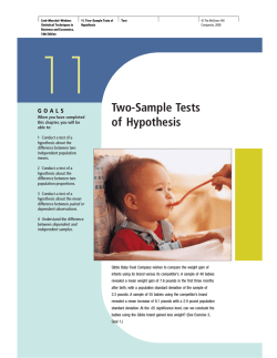
One- and Two-Sample
Tests of Hypotheses
10. 1 Statistical Hypotheses: General Concepts
Often. the problem confronting the scien tist or engineer is not so much the
estimation o f a population parameter as discussed in Chapter 9. but rather the
formation of a d a ta-based decision procedure that can prod uce a concl usion
about some scien tific system . For example. a medical researcher may decide
on the basis of experimental evidence whether coffee drinking incre ases the
risk o f cancer in h u m a ns; a n engineer might have to decide on the basis of samВ­
ple data whether t h ere is a difference between the accu racy of two kinds of
gauges: or a sociologist might wish to collect appropriate data to en able him
or her to decide whether a person's blood type and eye color are indepe ndent
variables. [n each o f these cases the scie n tist or engin eer postll/mes or conjecВ­
tllres something a bout a system. [n addition. each must involve the use of
experime ntal d ata and decision m aking that is based on the data. Formal ly. in
e ach case. the conjecture can be put in the form of a statistical hypothesis. ProВ­
ced u res t h a t lead to the acceptance or rejection of statistical hypotheses such
as these comprise a major area of statistical inference . First. let us de fine preВ­
cisely what we mean by a statistical hypothesis.
Dcfinilldll to.l
A statistical hypothesis is a n assertion or conjecture concerning one o r
m ore popUla t ions.
j
The truth or falsity of a statistical hypothesis is never k n own with absolute
certainty u nless we examine the entire popu l ation . This. o f course. would be
290
Section 10.1 Statistical Hypotheses: General Concepts
291
impractical in most situations. I nstead. we take a random sample from the popВ­
ulation of in terest a n d use (he data contained in this sample to provide eviВ­
dence that eith e r supports or does not support the hypothesis. E vidence from
the sample that is inconsiste n t with the stated h ypothesis lea ds to a rejection
of the hypothesis. where as evide nce supporting the hypothesis leads to its
acceptance.
It should be m a de clear to the reader that the design of a decision proceВ­
dure must be done with the notion in mind of the pro!Jabilil}' of (/ wrong COI/В­
clusion. For example. suppose that the conjecture (the hypothesis) postulated
by the engineer is that the fraction defective p in a certain process is 0.10. The
experime n t is to observe a ran dom sample of the product in 4uestion. Suppose
that 100 ite ms are tested and 12 i tems are found defective . Il is reasonable to
conclude tha t this evide nce does not refute the condition p = 0. 1n. and thus i t
m a y lea d to a n acceptance of t h e hypothesis. H owever. i t also does n o t refute
p = 0.12 or perh aps even p = 0.15. As a result. the reade r m u st be acclIsВ­
tomed to u n derstan ding th at the acceptance of a hypothesis merely implies
that the data do not give sufficient evidence to refute it. On the other hand,
rejection implies that the sample evidence refutes it.
Put another way.
rejecВ­
tion means that there is a small probability of obtaining the sample informaВ­
tion observed when, in fact, the hypothesis is true. For example. in our
proportion -defective h ypothesis. a sample of 100 revealing 20 defective items
is ce rtainly e vide nce of rejection. Why'? I f. indeed. p = 0.10. the proba bility of
obtaining 20 or more defectives is approximately 0.0035. With the resulting
small risk of a wrong cOl/clllsiol/. it would seem safe to reject the hypothesis
tha t p = 0. 1 0. In other words. rejection of a hypothesis It!ncls to all hut "rule
ouf' the h ypothesis. On the other hand. it is very important to emphasize that
the acceptance or. rather. failure to reject does not rule out other possihilities.
As a result. th e fir/ll conclusiol/ is established hy rhe dow (Il/lIlyst when II
hypothesis is rejected.
The formal statement of a h ypothesis is often influenced hy the structure
of the prohahility of a wrong conclusion. If the scientist is intereste d in strongly
supporting a contention. he or she hopes to arrive at the contention in the form
of rejection of a hypothesis. I f the me dical researcher wishes to show strong
evidence in favor of the contention that coffee drin king increases the risk of
cancer. the h ypothesis teste d should be of the form "the re is no increase in
cancer risk produced hy drin ki ng coffee." As a result. th e conten tion is
reached via a rejection. Similarly. to support the claim that one ki n d of gauge
is more accurate tha n another. the engineer tests the hypothesis that there is
no difference in the accuracy of th e two kin ds of gauges.
The .
and /Hternative Hvpotheses
The structure of hypothesis testing will be formulated with the use of the term
This refers to any h ypoth esis we wish to test and is denoted
hy Ho. The rej ection of HI) leads to the acceptance of an alternative hypotheВ­
sis. denoted by H I' A null h ypothesis concerning a population parameter will
null hypothesis.
292
Chapter 10
One- and Two-Sample Tests of Hypotheses
always be stated so as to specify an exact value of the paramete r, w he re as the
a l ternative hypothesis allows for the possibility of several va l ues. H ence, if HI)
is th e n u l l h ypothesis p = 0.5 for a binomial popul atio n , th e alte rn a tive
hypoth esis HI would be one of th e following:
p > 0.5,
p <
or,
0.5,
p =1=
0.5 .
10.2 Testing a Statistical Hypothesis
L.
To illustrate the concepts used in testing a statistical hypothesis about a popВ­
ulation, consider th e fo l lowing example. A ce rtain type of cold vaccin e is
known to be only 25% e ffective afte r a period of 2 years. To determine if a n e w
and somewhat more expensive vaccine is superior i n providing p rotection
against the same virus for a longer period of time , suppose that 20 people are
chosen at ran dom and inoculated. In a n actual study of this type the particiВ­
pan ts receiving th e new vaccine m ight number several thousand. The number
20 is being used h e re only to demonstrate the basic steps in carrying out a staВ­
tistical test. I f more than 8 of those receiving th e new vaccine surpass th e 2year period without contracting the virus, th e new vaccine will be considered
superior to the one presently in use. The requirement that the number exceed
8 is somewhat arbitrary but a ppears reasonable in that it represents a modest
gain over the 5 people that could be expected to receive protection if the 20
people had been inoculated with the vaccine already in use. We are essentially
testing the n u l l h ypothesis tha t the n e w vaccine is equal l y effective after a
pe riod of 2 years as the one now commonly used. The alternative hypoth esis
is that the n e w vaccine is in fact superior. This is e quivalent to testing the
hypothesis th at the binomial parameter for thl proba bil ity of a success on a
give n tria l is p = 1/4 against th e alternative that p > 1/-1-. This is usually writВ­
ten as follows:
p=
p>
I
4'
I
4'
The test statistic on which we base our decision is X. the number of indiВ­
viduals in our test group who receive protection from the new vaccine for a
pe riod of at least 2 years. The possible values of X. from () to 20, are divided
into two groups: those numbers less than or equal to 8 and those greater th an
8. All possible scores greater than 8 constitute the critical region, and all posВ­
sible scores less th an or e qual to 8 determine the acceptance region. The last
number th at we observe in passing from the acceptance region into the critical
region is called the critical value. I n our il lustration the critical va l ue is the numВ­
ber 8 . The refore, if x > 8, we reject Ho in favor of the alternative hypothesis
H I' I f x пїЅ 8, we accept Ho. This decision crite rion is illustrated in Figure 10.1.
The decision procedure j ust described could lead to either of two wrollg
conclusions. For instance , the n e w vaccine may be no bette r than the one now
293
Section 10.2 Te sting a Statistical Hypothesis
Accept Ho
I
0
(p=0.2)
2
I
7
.
Figure
I
8
I,
9
Reject
Ho
(p> 0.2)
I
10
1 0.1 Decision criterion for testing p
20
.
=
0.2 versus p
>
x
0.2.
in use and, for this particular randomly selected group of individuals, more
than 8 surpass the 2-year period without contracting the virus. We would be
committing a n error by rejecting HI) in favor of HI when. in fact, Ho is true.
Such an error is called a type I error.
l>efinitiun
111.2
Rejection of the n u ll h ypothesis w h e n it is true is called a type I
error.
A second kind of error is committed if 8 or fewer of the group surpass the
2-year period successful ly and we conclude that the new vaccine is no bette r
when it actu a l ly is better. I n this case we would accept HI) when it is false. This
is called a type II error.
Definition
10.3
Acceptance of the n ull hypothesis when it is false is called a
type
n error.
I n testing any s tatistical hypothesis, the re are four possible situations that
determine whether our decision is correct or in error. These four situations are
summarized in Table 10.1.
Table 1 0. 1
Possible Situations for Testing a Statistical Hypothesis
Ho Is true
Ho Is false
Accept HI)
Correct decision
Type II error
Reject HI)
Type I error
Correct decision
The probability of committing a type I error, also called the level of sigВ­
is denoted by the Greek letter a. I n our illustration, a type I error
will occur when more tha n 8 ind ividuals surpass the 2-year period without conВ­
tracting the virus using a new vaccine tha t is actually equiva len t to the one in
use. H ence, I f X is the n umber of individuals who remain free of the virus for
at least 2 years.
nificance,
a
=
P(type I error) = P
=
I
-
Lh
K
\=0
(
x;
20,
)
(
X > 8 when p
1
= I
4
-.
-
I
= -
4
)
=
21)
Lb
.\=9
(
"
.
x;
20 .
1
.-
4
)
0.9591 = 0.0409.
We say that the n u l l h ypothesis. p = 1/4. is being tested at the a = (l.O409
level of significance. Sometime s the l e ve l of significance is called the size of
2:}:'$
Chapter 10
One- and Two-Sample Tests of Hvpotheses
the critical region. A critical region of size 0.0409 is very small and therefore
it is u n likel y that a type I error wi l l be com mitted. Consequently, it would be
most unusual for more th a n 8 in dividuals to remain i m mune to a virus for a
2-year period using a new vaccine tha t is essentially equivalent to the one now
on the market.
The probability of committ i ng a type II error, denoted by (3, is impossible
to compute u nless we have a specific alternative hypothesis. I f we test the null
hypothesis that p = 1/4 against the alternative hypothesis that p = 1/2, then
we are able to com pute the probability of accepting Ho w he n it is false. We
simply find the probability of obtaining 8 or fewer in the group that surpass
the 2-year period when p == 1/2. I n this case
f3 = P(type II error) =
p(x,,;:
8 whe n p =
i) пїЅ (
=
I
b X; 20,
i)
==
0. 2517 .
This is a rather h ig h probability. indicating a test procedure in wh ich i t is quite
likely that we shall reject the new vaccine when, i n fact, it is superior to tha t
n o w i n use . I de a l ly, w e like to use a test procedure for which both the type I
and type I I errors are small.
I t is possible that the director of the testing program is willing to make a
type II error if th e more expensive vaccine is not significantly superior. I n fact
the on l y time he wishes to g uard against the t ype If error is when the true
value of p is a t least 0.7. If p = 0.7. th i s test procedure gives
f3 = P(type II error)
P(X";: 8 when p = 0.7) =
=
x
2: b(x; 20. 0.7) = 0.0051.
r=--O
With such a small probabil i ty of com mitting a type II error. it is extremely
unlikely th at the new vacci ne would be rejected when it is 70o/r effective after
a period of 2 years. As the alternative h ypothesis approaches unity. the val ue
of {3 diminishes to zero.
Let us assume tha t the director of the testi n g program is unwilling to com В­
mit a type [ [ error when th e al ternati ve h ypothesis p == 1/2 is true e ven though
we have found the probabil ity of such an error to be f3 == 0. 2517. A reduction
in f3 is always possible by increasing the size of the critical region. For examВ­
ple . consider what happe ns to the values of Cl' and {3 when we change our critВ­
ical value to 7 so that all score s greater than 7 fall in the criti cal region and
those Jess th an or equal to 7 fall i n the acceptance regi on. Now. in testi ng
p = 1/4 aga inst the alternat ive h ypothesis th at p = 1/2. we fi n d that
Cl' =
and
'II
2: h
\
_.пїЅ
(
x;
I
20. '
4
)
= 1
f3 =
-
2: b
\
7
пїЅ(]
(
x:
В± h(X: 1)'
20,
\
пїЅII
'
I
)
20. - = 1 - 0.8982 = 0. 1018
4
2
=
0.1316.
By adopting a new decision procedure. we have reduced the probability
of committing a type II error at the expense of increasing the probability of
Section 10.2
Te sting a Statistical Hypothesis
295
committing a type I error. For a fixed sample size, a decrease in the probabilВ­
ity of one error will usually resul t in an increase in the probability of the other
error. Fortunately, the probability of com mitting both types of error can be
reduced by increasing the sampie size. Con sider the same problem using a ranВ­
dom sample of 100 individuals. If more than 36 of the group surpass th e 2-year
period, we rej ec t the n u ll h ypothesis that p = 1/4 and accept the alternative
h ypothesis that p > 1/4. The critical value is now 36. A l l possible scores above
36 constitute the critical region an d all possible scores l ess than or equal to 36
fall in the acceptan ce region.
To determine the probab ility of committing a type I error, we shall use
the normal -curve approximation with
J.L
= np = (lOO)(пїЅ) = 25
and
vnpq =
(T =
V(100)(пїЅ)(пїЅ)
=
4.33.
Referring to Figure 10.2, we need the area u nder the normal curve to th e right
of x = 36.5. The corresponding z-value is
z
36.5 - 25
=---4.-n- =
2.66.
пїЅ
----------------
пїЅ
пїЅ
пїЅ------
tL = 25
Figure
10.2 Probability of a type
From Table A.3 we find that
0' =
=
p(type I error)
=
1 - P(Z < 2.66)
p(X
=
I
=
пїЅ- x
error.
> 36 when p =
1 - 0.996 1
--
пїЅ)
=P(Z > 2,66)
0.0039.
I f Ho is false and th e true value of H I is p = 1/2, we can determine the
probability of a type I I error using the normal -curve approximation with
J.L =
np = ( 1 00)(пїЅ) =
50
and
(T
= vnpq =
. пїЅ ..
V(100)( I )6I ) = 5.
2
The probability of falling in the acceptance region when H I is true is given by
the area of the shaded region to the l eft of x = 36.5 in Figure 10.3. The z-value
correspon ding to x = 36.5 is
z
36.5 - 50
= -5--=
-
2.7.
-
296
Chapter 10 One- and Two-Sample Tests of Hypotheses
(T=
5
/
____________ __
-LI
25
-L------------ x
----------------------
Figure
There fore,
f3
=
P(type I I error) =
50
1 0.3 Proba b i l ity of a type II e r ror.
p(
X пїЅ 36 when p =
D
=
P(Z <
-
2.7) = 0.0035.
O bviously, the type I and type I I errors will rarely occur if the experiment conВ­
sists of 100 individuals.
The illustration above u n derscores the strategy of the sci entist in hypothВ­
esis testing. A fter the null and alternative h ypotheses are stated, it is i mporВ­
ta n t to consider the sensitivity of the test procedure . By this we mean that
t here should be a determi nation, for a fixed (1' , of a reasonable value for th e
probability of wro ngly accepti ng HI! (i.e .. the value of (3) when th e true situaВ­
ti on represents some imporlilnt del'iafioll frolll H11. The value of the samole
size can usually be de termined for which there is a re as onab le balance
he twee n i t and the \alue of f3 c ompu te d in this fashion. Th e v acci ne probl e m
is an illustration.
The cOllcepts discussed here for a discrete popUlation can equally well be
applied to continuous popUlations. Consider the null hypothesis that the averВ­
age weight of male student-. in a certain college is oX kilograms against the
,i 1ternati\e hypothesis
that It is une q u al to oK That is. we wish to test
1111 :
/1
1/1:
/-i
=
=1=
fiX,
()x.
The alternative hypothesis allows for the possihility that /1 '
A sample mean that falls close
oX or /1 -> flS.
the hypothesized value of fiX would
to
be
is
considL'/'ed evidence in favor of fill' On the other ham!. a sample mean that
considerably less than or more than IlX
ul d he
wo
evidence inconsistent with IlII
and therefore favoring 111' The "ample mean is t h e test statistic in thi s case. A
critical region for the test statistic might arh it rar ily be chosen t o
be t he tw o
i nt er vals .r < 67 and .r > flY. T he ,lCceptance region will th en he t he interval
67 % x "" 6Y. This decision criterion is illustrated in F i gur e lOA.
Ho
(JL # 68)
Reject
Accept
(f..'
67
Figure 10.4
=
Ho
Reject Ho
(JL # 68)
68)
68
Probab i lity of a type
69
II
e r ror.
Section 10.2
Testing a Statistical Hypothesis
297
Let us now use the decision criterion of Figure 10.4 to calculate the probВ­
abilities of committing type I and type I I errors when testing the null hypothВ­
esis that J.L = 68 kilograms against the alternative that J.L =1= 68 ki lograms for
the continuous population of students' weights.
Assume the standard deviation of the population of weights to be
(T = 3.6. For large samples we may substitute s for (T if no other estimate of (T
is avail aQ le. Our decision statistic, based on a random sample of size n = 36,
will be X, the most efficient estimator of J.L. From the central limit theorem,
we know that the sampling distribution of X is approximately normal with
standard deviation (Tx (T/ Vii = 3.6/6 = 0.6.
The probability of committing a type I e rror, or the level of significance
of our test, is equal to the sum of the areas that have been shaded in each tail
of the distribution in Figure 1 0.5. Therefore,
=
a =
P(X < 67 when J.L
=
68)
+
P(X > 69 when J.L = 68 ).
пїЅ-------L--пїЅ--пїЅпїЅ-- x
69
67
Figure
1 0.5 Critical region for testing
The z-values corresponding to Xl =
Zl
=
67 - 68
-0.6""
=
-
1 .67
J.L = 68
67 and x2
and
versus
=
69 when
Z2
=
J.L
*
68.
flo is true are
69 - 68
(iпїЅ6
=
1 .67.
The refore,
a =
P(Z
<
- 1 .67)
+
P(Z
>
1 .67) = 2P(Z
- 1 .67)
<
=
0.0950.
Thus 9.5 % of all samples of size 36 would lead us to reject J.L = 68 k ilograms
when it is true . To reduce a, we have a choice of increasing the sample size or
widening the acceptance region. Suppose that we increase the sample size to
n = 64. Then (Tx = 3.6/8 = 0.45. N ow
пїЅ =
"I
67 - 68
0.45
...
...
"
=
-
2.22
and
Z2 =
69 - 68
. ... .. = 2.22.
0.45
"
H ence
a =
P(Z
<
- 2.22)
+
P(Z > 2.22) = 2P(Z
<
- 2.22)
=
0.0264.
The reduction in a is not sufficient by itself to guarantee a good testing
procedure. We must eval uate f3 for various alternative hypotheses that we feel
should be accepted if true . Therefore, if it is important to reject Ho when the
298
Chapter 10 One- and Two-Sample Tests of Hvpotheses
true mean is some va lue f.L пїЅ 70 or f.L пїЅ 66, then the prohahility of committing
a type I I error should he computed and examined for the altern atives f.L == 66
and f.L = 70. Because of sym m e try, it is only necessary to consider the prohaВ­
hility of accepting the n ull hypothesis that f.L == 68 when the alternative f.L == 70
is true. A type I I error will result when the sampl e mean _r falls he tween 67 and
69 when HI is true. Therefore, referring to Figure 10.6. we find that
f3 == P(67 пїЅ X пїЅ 69 when f.L == 70).
В·,Ho
пїЅ____________IL______ X
________
67
Figure
70
69
68
10.6 Type" error for testin g
The z-values corresponding to
68 versus
J1. =
70.
and x2 == 69 when HI is true are
.rl == 67
67 - 70
Z I == - -- -- == - 6.67
0.45
J1. =
Z2 =
and
69 - 70
- - == - 2.22.
0.45
-пїЅ
Therefore.
f3 == P( - 6.67 < Z < - 2 .22)
== 0.0132 -
JI
f
!t
=
P(Z < - 2.22) - P(Z < - 6.(7)
O.O()OO = 0.0132.
If the t rue va lue of f.L is the alternative f.L == 66. the va lue of f3 wi ll again
he 0.0132. For all plissi hle values of f.L < fJ6 or f.L > 70. the value of f3 will he
even smaller when 11 == 64. and consequently there would he little chance of
accept ing H(( when it is false.
The prohahility of committing a type [[ error in creases rapi dly when the true
value of f.L approaches. hut is not eq ual to. the hypothesized value. Of course. this
is usually the situation where we do not mind maki ng a type" error. For example.
if the alternative h ypoth esis f.L == 6:-;.5 is true. we do not mind commit! ing. a type [[
error by concludi ng that the true answer is f.L == 6k. The prohabi li t y of making
such an error \vi ll be high when 11
64. Referring to Figure 10. 7. we have
==
f3 == P(67 пїЅ X пїЅ 69 when f.L == 6k.5).
H,
---LI
________
67
Figure
I
(
I
--'-I
...JIL-__
68
...JI
__
68.5
1 0.7 Type II error for testin g
____
69
J1. =
68 versus
!.L
x
=
68.5.
299
Section 10.2 Te sting a Statistical Hypothesis
The z-values corresponding to.t] =
z
]
=
67 - 68.5
0.45
.------
=
67 and .t2
- 3. 33
=
69 when JJ..
Z2 =
and
=
69 - 68.5
'
0.45
.
68.5 are
= 1.11.
Therefore,
f3 =
=
P( - 3.33 <
Z <
0.8665 - 0.0004
1. l 1)
=
=
P(Z
<
1 .11) - P(Z
<
- 3.33)
0.866 1 .
The preceding examples illustrate the following important properties:
1. The type I e rror and type I I error are re lated. A decrease in the probabilВ­
ity of one generally results in an increase in the probability of the other.
2. The size of the critical region, and therefore the probability of committing
a type I error, can always be reduced by adj usting the critical value(s).
3. A n increase in the sample size n will reduce
Q'
and {3 simul taneously.
4. If the n u l l hyphothesis is false, {3 is a maximum when the true value of
a parameter approaches the hypothesized value. The greater the disВ­
tance between the true value and the hypothesized value, the smaller
{3 will be.
One very i mportant concept that relates to error probabil i ties is the
notion of the power of a test.
Definition lOA
I пїЅпїЅпїЅпїЅ
IT he power of a test is the probability of rejecting Ho given that a specific
tive is true .
_
__
_
_
The power of a test can be computed as I - {3. Often different types of
tests are compared by contrasting power properties. Consider the previous
illustration in wh ich we were testing Ho: JJ.. = 68 and HI: JJ.. 1= 68. As before,
suppose we are interested in assessing the sensitivity of the test. The test is govВ­
erned by the rule that we accept if 67 :!S X пїЅ 69. We seek the capability of the
test for properly rejecting Ho when indeed JJ.. = 68.5. We have seen that the
probabil ity of a type I I error is given by f3 = 0.866 1 . Thus the power of the test
is 1 - 0.866 1 = 0. 1 339. In a sense , the power is a more succinct measure of
how sensitive the test is for "detecting differences" between a mean of 68 and
68.5. I n this case, if JJ.. is truly 68.5, the test as described will properly reject Hn
only 13.39% of (he iime. As a result, the test would not be a good one if it is
important that the analyst h ave a reasonable chance of truly distinguishing
between a mean of 68.0 (specified by Ho) and a mean of 68.5. From the foreВ­
going, it is clear that to produce a desirable power (say, greater than 0.8), one
must either increase Q' or increase the sample size.
In what has preceded in this chapter, much of the text on hypothesis testВ­
ing revolves around foundations and definitions. I n t he sections that foll ow we
get more specific and put hypotheses in categories as well as discuss tests of
300
Chapter 10
One- and Two-Sample Tests of Hvpotheses
h ypotheses on various parameters of i n terest. We begin by drawing th e disВ­
tinction between a one-sided and two-sided h ypoth esis.
10.3 One- and Two-Tailed Tests
A
test of any statistical hypoth esis, where the alternative is
Ho:
8 = 81i,
HI:
8> 80,
or perhaps
Ho:
8 = 80,
lfl :
8 < 811,
one-sided,
such as
is called a one-tailed test.
I n Section 10.2, we make reference to th e test statistic for a h ypoth esis.
General ly, the criti cal region for the alternative hypoth esis 8> 80 lies in th e
rig h t tai l of th e distribution of th e test statistic, wh i l e the criti cal region for
th e alternative hypothesis 8 < ell l i es entirely in th e left tai l . In a sense, th e
inequal i ty symbol poin ts i n th e direction where the critical regi on l ies. A on eВ­
tai led test is used in the vaccine experime n t of Section 10.2 to test the h ypothВ­
esis p = 1/4 agai nst th e on e-s i de d alternative p > 1/4 for the bi nomial
distri bution. Th e one-tai l e d criti cal region is usual l y obvious. For an underВ­
standing the reader should visual i ze the beh avior of th e test statistic an d
notice th e obvious siRna/ that wou l d produce evidence supporti ng th e alterВ­
native hypothesis.
A test of any statistical hypothesis where the alternative is two-sided, such as
t
I
is cal led a two-tailed test, si nce the critical region is spl i t into two parts, ofte n
having e qual probabi l ities placed in each t<lil of the distribution of the test staВ­
tistic. The alternative hypothesis H =1= Ho sUltes that either H < 811 or H > HII• A
two-tai l e d test was used to test the n u l l hypothsis that f..t = 61-1 kilograms
agai nst the two-sided alternative f..t =1= 61-1 kilograms for the contin uous popuВ­
lation of student weights in Section 10.2.
The null hypothes is, HII, will always be stated using the eLju al ity sign so as
to specify a single val ue. In th is way the probability of committing a type I
error can be control led. Whe th er one sets up a one-tai l ed or a two-tai led test
wi l l depend on the conclusion to be drawn if Ho i s rejected. The l ocation of th e
critical region can be determi n ed on ly after HI h as been stated. For exampl e,
i n testi ng a new drug, on e sets up the hypoth esis that it is no better than simВ­
ilar drugs now on the market and tests this agai nst the alternative hypoth esis
that the new drug is superior. Such an alternative hypoth esis wi l l result in a
on e-tail ed test with the critical region in the right tai l. However, if we wish to
compare a n e w teach ing techn ique w i th the conven tional classroom proceВ­
dure, the alternative hypothesis shou l d al low for the new approach to be either
inferior or superi or to the conventional procedure. Hence th e test is two-tai led
Section 10.3 One- and Two-Tailed Tests
301
wi th the critical region divided equally so as to fal l in the extreme left and right
tai ls of the distribution of our statistic.
Certain guidelines are desirable in determining which hypothesis should
be stated as Ho and which should be stated as HI . First, read the problem careВ­
ful ly and determine the claim that you want to test. Should the claim suggest
a simple direction such as more than, less than, superior to, inferior to, and so
on, then HI wil l be stated using the inequality symbol ( < or > ) correspondВ­
ing to the suggested direction. If, for example, in testing a new drug we wish
to show strong evidence that more than 30% of the people will be helped, we
immediately write HI: p > 0.3 and then the n u l l hypothesis is written Ho:
p = 0.3. Should the claim suggest a compound direction (equality as well as
direction) such as at least, equal to or greater, at most, no more than, and so on,
then this entire compoun d direction ( пїЅ or пїЅ ) is expressed as Ho' but using
only the equality sign , and HI is given by the opposite direction. Finally, if no
direction wh atsoever is suggested by the claim, then HI is stated using the not
equal symbol ( *- ) .
Example 10.1 A man ufacturer of a certain brand of rice cereal claims that
the average saturated fat conte nt does not exceed 1.5 grams. State the null and
alternative hypotheses to be used in testing this claim and determine where
the critical region is located.
SOLUTION
The manufacturer's claim should be rejected only if J-L is greater than 1.5 milВ­
ligrams and should be accepted if J-L is less than or equal to 1.5 milligrams.
Since the null hypothesis always specifies a single value of the parameter, we
test
Ho :
J-L = 1.5,
H I:
J-L> 1.5.
A lthough we have stated the null hypothesis with an equal sign, it is underВ­
stood to inc lude any value not specified by the alternative hypothesis. ConseВ­
q uently, the acceptance of HI! does not imply that J-L is exactly equal to 1.5
mi lligrams but rather that we do n ot h ave sufficient evidence favoring HI'
Since we have a one-tailed test, the greater than symbol indicates that the critВ­
iВЈa l region lies entirely in the right tail of the distribution of our test statistic
X.
•
Example 10.2
A real estate agent claims that 60% of all private residences
being bui l t today are 3-bedroom homes. To test this claim, a large sample of
new residences is inspected: the proportion of these homes with 3 bedrooms
is recorded and used as our test statistic. State the null and alternative
hypotheses 10 be used in this test and determine the 10catio'1 of the critical
region.
SOLUTION
If the test statistic is substanti a l ly higher or lower than p = 0.6, we would
reject the agent's claim. Hence we should m ake the hypothesis
302
Chapter 10
One- and Two-Sample Tests of Hvpotheses
Ho :
P = 0.6,
iii:
P *- 0.6.
The a l ternative hypothesis implies a two-tailed t пїЅst with the crit ical region
divided equal l y in both tails of the distribution of p, our test statistic.
10.4 The Use of P-Values for Decision Making
In testing hypoth e ses in which the test statistic is discrete, t h e critical region
may be chosen arbitrarily a n d its size determined. If a is too large, it can be
reduced by making an adjustment in the critical val ue. I t may be n ecessary to
increase the sampl e size to offset the decrease that occurs automatical l y in the
power of t h e test.
Over a number of gen erations of statistical analysis, it had become cusВ­
tomary to choose an a of 0.05 or 0.0 I and select th e critical region accordingly.
Then , of course, strict rejection or nonrejection of HIJ wou l d depen d on tha t
critical region. For example. i f t h e test is two-t ail ed and (Y is set a t the 0.1)) leve l
of significance and the test statistic invol ves, say, the sta n dard normal distribВ­
ution, then a z-va lue is observed from the data and the critical region is
z > 1.96.
z <
-
1.96,
where the va lue 1.96 is found as ZIl.II.:'5 in Table A .3. A value of :: in the critical
region prompts t h e state ment: 'The val ue of t h e test sta tistic is significant."
We can translate that into the user's la nguage . For example. if the h ypot hesis
is given by
J
fill:
f.L = 10,
"I:
f.L =to 10.
one might say: "The mean differs sign ifica ntly from the va lue 10."
This preselection of a significance level a has its roots in the philosophy
that the maximum risk of making a type [ error should be controlled. HowВ­
ever. this approach does not account for values of test statistics that are "c1ose"
to the critical region. Suppose. for example, in t h e il l u stnltion wit h /II':
f.L = 10: III: f.L *- 10, a va lue of z = I.k7 is ohserved: strictly spea king, with
a = 0.0) the va lue is not significant. But the risk of cummit ting a t ype I e rror
if on e rejects iii I in t h is case cou l d hardly be con sidered severe. In fac t . in a
two-tailed scenario one can quantify t h is risk as
P = 2P(z >
UP
when f.L = 10) = 2(0.0307) = 0,0614.
As a resu l t . 0,0614 is the probabil it y of ohtaining a va l ue of z as large or larger
(in magnitude) than l.k7 wh en in fact f.L = 10. Although this evidence against
fill is not as strong as that which would resu l t from a rejection at an a = 0.0)
le vel . it is important information to t h e user. I n deed. comin ued use o f
a = O.OS or 0.0 I i s only a result of what standards have b e e n passed t h rough
the generations. The P-value approach has been adopted extensively by users
Section
10.4 The Use of P-Values for Decision Making
303
in applied statistics. The approach is designed to give the user an alternative
(in terms of a probability) to a mere "reject" or "do not reject" conclusion.
The P-value computation also gives the user important information when the
z-value falls well into the ordinary critical region. For example, if z is 2.73, it is
informative for the user to observe that
P =
2(0.0032)
=
0.0064
and thus the z-value is significant at a level considerably l ess than 0.05. It is
important to k now that under the condition of Ho. a value of z = 2.73 is an
extremely rare even t. N amely, a value at least that large in magnitude wou l d
o n l y occur 64 times in 1 0.000 experiments.
One very simple way of explaining a P-value graphically is to consider two
distinct samples prematurely. Suppose that two materials are considered for
coating a particular type of metal in order to inh ibit corrosion. Specimens are
obtained and one co flection is coated with material 1 and one collection coated
with material 2. The sample sizes are n,
n2
10 for each sample and corroВ­
sion was measured in percent of surface area affected. The hypothesis is that
the samples came from common distributions with mean Ji = 1 0. Let us
assume that t he population variance is 1 .0. Then we are testing
=
Ho:
Ji, = Ji2
=
=
1 0.
Let Figure 10.8 represent a point plot of the data; the data are placed on
the distribution stated by the null hypothesis. Now it seems clear that the data
do refute the null hypothesis. But how can this be summarized in one number?
The P-value can be viewed as simply the probability of obtaining this data set
given that the samples come from the distribution depicted. Clearly. this probВ­
abi l ity is quite small. say 0.00000001 ! Thus the small P-value clearly refutes
Ho. and the conclusion is that the population means are significantly different.
J.L
Figure
=
10
v,
1 0.8 Data that are likely generated from populations having two different means.
The P-val ue approach as an aid in decision m a king is quite natural
because nearly all computer packages that provide hypothesis-testing compuВ­
tation print out P-values along with values of the appropriate test statistic. The
fol lowing is a formal definition of a P-value.
Detinition 10.5
[
A P-value is the lowest level (of significance) at which the observed value
of the test statistic is significant.
Chapter 10 One, and Two-Sample Tests of Hypotheses
304
It might be appropriate at this poi n t to s u m marize the procedures f(
h ypoth e<;i s testing, This may serve as a foun dation on which specia l cases ar
ha sed in sllcceeding sections, For this summary, assume that the hypothesis i
fI,,: 8
80,
==
l. State the n u l l hypothesis 110 that H
HIl,
==
2. Choose an appropriate alternative hypothesis III from one of the allerna
tives H < HI)' H> 80, or H '* HII,
3. Choose a significance l evel of size
(\"
4. Select the appropriate test statistic and establish the crit ica l region, (If the
decision is to h e hased o n a P-value, it is not necessary t o slate the critical
region,)
5. C o m p ut e
the value of the test statistic from the sample da ta,
6. Decision: Reject /III if the test statistic has a value in t he nit ical re!!ion (or
if the co mputed P-value is less than or equal to
l eve I a): ot herwise, do not reject /10'
the desired si.\!nific<1nce
The reader should realize that the conclusions drawn hy the analyst illay
affected hy computed P-val ues, In other words, one may Ih)t have a preseВ­
lected (Y level in mind and thus draw conclusions hased on t h e information proВ­
v i d e d hy the P-value, As indicated earlier. this is the approach often taken in
rL'a l-lifc situations,
he
Exercises
1, ."lIl'l't"пїЅ' IhпїЅ11
hll'"llh>h 111;11 <II
''''llc
l"
,1Il ;lilerпїЅisl wiпїЅhes 1 0 lest Ihe
k,r" 30'/; III' Ihe publie is ; d ler,!! i c 10
,'IIC'l"l' !,luclllCf';, r::',pl"in hm\' the ,iIlergisl could
"111/1111
(" I it 1\ Pl' I ,:1" , ),:
1.1', ,I 111'c' 1I,'IT,n,
clucle Ihill
2, ,\" 'l'i, ll()пїЅпїЅi'l IS cdllll'rncd ah()lIt Ihl' dkclivelless
,JI " Ir"i"",пїЅ. l'\lIIr,,: ,k,,,!nl'd In gel mure driver, 10
lI'" ,c,11 I'vlh in ,1111'''llOIВ·i\c-s,
(II WIi<l1 11II'(I\I1L" " is ,he ic'sting il Sill.' cOl11mits a
II I'c' I c'rr,,, hI cr"'llc',ll"'" ""Ilcilldin!! Ihal Ihe tr<linВ­
InпїЅ (lIIISl' i, inelleclill'"
(I>I \\ kit III Jl"lhL',is i, she ic' sl in g if she cOlllmits a
Ilpc II c'ITIlr I" CITlllh:"lIslll'IIncilitiin!I Ihal Ihe t rain В­
in!! C,'l!rSl' is ciTcclivc.'
3, :\ larпїЅ,' l11anliLICIUril1!I firlll is hein!I chargeu wilh
dis,'li11lilldll<"i in ih hiring
random sample or 1.пїЅ ,Idults
sclectcd, II" the numher 1'1' c o llc ge !Ir"dLlil"" in OUI
samp le is anywherc frolll h 10 12, Ill' shall "ccepi the
null hypolhesis Ihal f!
O,h: lHilerllisl', we ,h;1I1 (IlnВ­
To test this hypothesis, a
is
praclices,
(,I) \\ h;)1 11I1"lihl'sis is hrin)! tested if a jury commits
:1 111'c I c'ITIII I" fillding Ihc rinn guill\'"
(h I \\ 11<11 1111" ,t hl'sis is heill)! lested i I' a j lIry Clllllll1its
:l III'" II ':1'1'" III finding Ihe firm guillv','
4, 'Ill<: 1"III'(lrli"'l "I' "dults liling in a small tuwn
l\ohl) <Ire c()lk!!l' g r ad l l <lles is eslil11<lted 10 he p
O,n,
=
f! пїЅ O,h
(;1) r:v,tiuate
If
=
assliming
Ihal
mial disirihulillll,
(hI haluate {3lor Ihe alkrniltil'c
(c) b Ihis
I I ()
the
"пїЅ ,\ -s
uilles
in
/1
пїЅooJ IeSI prllcedure')
5, Repc'at L\ercise пїЅ
nd
il
<l
0,(" l\,' lile' bint)В­
[I
"ccCptilI1Cl'
II hell
..'Ii() "dull,
our silmple , l:,c Ihe
;Irc'
IU.
sl'le-clL'd
1(\ he
Iltlmhcr "f c, likпїЅL' gI"dВ·
rc!!i'll1
130 IIherL'.r is Ihe
(1.:" ,lI1d /'
is
defincd
nllrm,t1 ilppro\irnill i'ln,
6, A filhric n1<lnUraclurcr helicvcs thill the
IH')jl"r'
OJ),
II' a random sample of I () l )rders shows Ihal 3 or Icwer
arrived lale, the hl'polhesis Ihal I'
O,h should he
rej ecled in favor Ilf Ihe allernillil'c f1' O,h, Usc Ihe
lion or orders for rilW ll1atcri:iI ilrrilВ·in!:'. lale is
/)
пїЅc
'=
binomial distrihution,
il Ivpe I error
J! ,0 O,h.
(h) Find the p robahili l Y or Ctlillmiiting il Ilpc II errllr
for the alternalive p = tI.3,/)
OA, and [)
O,S,
(a) Find thc prohahilil\' or COllllllillil1)!
ir t he I rue proporlilln is
=
=
Section
7. Repeat Exercise 6 when 50 orders are selected,
and t h e critical region is defined to he
x пїЅ
24. where
x i s the number of orders i n our sample that arrived
late. Use the normal approximation.
8. A dry cleaning establishment claims that a new
spot remover will remove more than 70o/c of t h e spots
10.4 The Use of P-Values for Decision Making
305
of 15 k i lograms with a standard deviation o f 0.5 kiloВ­
gra m . To test t h e hypothesis that J.t = 1 5 kilograms
against the alternative that J.t < 1 5 kilograms, a ranВ­
dom sample of 50 l i n e s will be tested. The critical
region i s d e fi n e d to be x < 1 4.9. Assume
correct.
u ==
15 i s
to which it is applie d . To check this claim. the spot
(a) Find the probability of committing a type I t!rror
remover will be used on 12 spots chosen at random.
when H() is true .
I f fewer than 1 1 of the spots are remove d , we s h a l l
accept the n ul l hypothesis that p = 0 . 7 ; otherwise,
we conclude that p > 0.7.
( a ) Evaluate
a,
assuming that p = 0.7.
(h) Evaluate f3 for t h e alternative p = 0.9.
9. Repeat Exercise 8 when 100 spots are treated and
the critical region is defined to be x > 82 , where x is
the numher of spots removed.
( h ) Evalu att! f3 for t h e altt!rnat ivcs J.t = 1 4 .8 and
f.L = 1 4.9 k i lograms.
1 5 , A soft-drink machine at a stt!ak house is reguВ­
lated so that the amount of dri n k dispensed is approxВ­
i m att!ly norma l l y distributed with a mean of 200
m i ll i l it e rs and a s t a n d ard deviation of 1 5 m i l l i l iters.
The machine is cht!cked periodically hy taking a samВ­
pit! of 9 drinks a n d computing the average content. If
1 0. I n the publication Relief from A rthritis by ThorВ­
i falls i n t h e i n t erval 1 9 1 < :t' < 209, t h e machine i s
40% of the sufferers from osteoarthritis received meaВ­
conclude t h a t f.L '* 2 00 milliliters.
ticular species of m ussel found off the coast of New
when f.L = 200 m i l l iliters.
sons Puhl ishers. Ltd . . John E. Croft claims that over
surable relief from a n ingredient produced hy a parВ­
Zealand. To test this claim. t h e mussel extract is to be
given to a group of 7 osteoarthritic patients. If 3 or
more of the patients receive relief. we shall accept the
null hypothesis t h at p = 0.4: otherwise. we conclude
that p < 0.4.
(a) Evaluate
a.
assuming that p = 0.4.
( b ) Evaluate f3 for the alternative p = 0.3.
1 1 . Repeat Exercise 1 0 when 70 patie nts are given
the m ussel ext ract a n d the critical region is defined to
be x < 24. where
x
is the n umber of osteoa rthritic
patients who receive relief.
12. A random sample of 400 voters in a certain city are
asked if they favor an additional 4'k gasoline sales tax
to provide hadly needed revenues for street repairs. If
more than 220 but fewer than 260 favor the sales tax,
we shal l conclude that 60'/r of the voters arc for it.
(a) Find t h e prohahility of co mmitting a type 1 error
i f 60% of the voters favor the increased tax.
(h) What is t h e prohability of comm i t t i ng a type II
error using this test procedure if actually only 48% of
t h e voters are in favor of the additional gasolinc tax?
13. Suppose, in Exercise 1 2, we conclude that 60% of
t h e voters favor t h e gaso l i n e sales tax i f more t h a n
2 1 4 b u t fewer t h a n 2 6 6 voters in o u r sample favor i t .
Show that this n e w acceptance region results i n a
smaller value for
a
at the expense of increasing f3.
1 4 . A m a n u facturer h a s developed a new fishing
l i n e , which he claims has a mean breaking strength
thought to h e operating satisfactorily: otherwise. w e
( a ) Find the prohability of com mitting a type I error
(b) Find the probability of committing a type II error
when f.L = 2 1 5 milliliters.
1 6 . Repeat Exercise 1 5 for samples of size
Use the same critical region.
II =
25.
1 7 . A new cure has been developed for a certain type
of cement that resu l ts i n a compressive strength of
5000 kilograms per square centimeter and a standard
deviation of 1 20. To test the hypothesis t h at f.L = 5000
against t h e alternative t h at f.L < 5000, a random samВ­
ple of 50 pieces of cement is teste d . The critical region
is defined to be x < 4970.
( a ) Find the probahility of committing a type I error
when Hu is true.
( b ) Eval uate f3 for t h e al ternat ive JL = 4970 and
f.L = 4960.
1 8. If we plot the prohabilities of acce p t i ng HI) corВ­
responding to various alternatives for f.L (including
the value specified by Hu ) and connect all the points
hy a smooth curve, we obtain the operating characВ­
teristic curve of the test criterion, or simply the O C
curve. Note that t h e prohability of accepting Hu when
it is true is s i mply 1
-
a.
Operati n g characteristic
curves are widely used i n ind ustrial applications to
provide a visu a l display of the merits of the test criteВ­
rion. With reference to Exercise I S , find the probaВ­
hilities of accepting Hu for the fol lowing 9 values of f.L
and plot the OC curve: 1 84, 1 88, 1 92 , 1 96. 200. 204,
208, 2 1 2, and 2 1 6.
306
Chapter 10 One- and Two-Sample Tests of Hvpotheses
1 0. 5 Single Sample: Tests Concerning a Single Mean
(Variance Known)
I n this section we consider formally tests of hypotheses on a single populaВ­
tion mean. Many of the illustrations from previous sections involved tests on
the mean. so the reader should already have insight i nto some of the detai ls
that are outlined here . We should first describe the assumptions on wh ich
the e xperiment is based. The model for the underlying situation centers
around an experiment with X l . X2 • . • . • XIl representing a random sample
from a distribution with mean J-L and varia nce (T 2 > O . Consider first the
hypothesis
Ho :
J-L == J-Lo .
HI :
J-L =1= J-Lo '
The appropriate test statistic should be based o n t h e random variable X. I n
Chapter 8 . the central l imit theorem i s introduced, пїЅhich essentially states that
despite the distribution of X, the random variable X has approximately a norВ­
mal distribution with mean J-L and variance (T 2 /f1 for reasonably large sample
sizes. So, J-Lx = J-L and (TпїЅ = (T2/n. We can then determine a critical region
based on the computed sample average, X. It shou ld be clear to the reader by
now that there will be a two-tailed critical region for the test.
It is convenient to standardize X and formally involve the standard nOfВ­
mal random variable Z. where
Z
= (T/'v
X - J-L
..
...
n
.
We know that lInder HI ) , that is. if J-L = J-LI ) . then ( X
N(O. 1 ) distribution. and hence the expression
P
(
7 (t Il
- ""
,.
<
пїЅ
-
/
J-Lo
CT \ /1
<
7
,
,-
"' n / ")
)
= 1
- J-LlI )/(T/'v
/1
has an
- 0'
can be used to write an appropriate acceptance region. The reader should keep
in mind that, formally, the critical region is designed to contro l 0', the probaВ­
bi lity of type I error. It should be obvious that a two-tailed signal of evidence
is needed to support HI ' Thus, given a computed value x, the formal test
involves rejecting Ho if the computed test statistic
Z ==
.-.- .. .
x
J-L()
>
(T/Yn
.
Z a/_"
or
Z
<
- Z,,/2 '
If - Z a /2 < Z < Z ,, /2 ' do not reject H() . Rejection of Ho , of course. implies
acceptance of the a lternative hypothesis J-L =1= J-Lo . With this definition of the
Section 10.5 Single Sample: Tests Concerning a Single Mean (Variance Known)
307
critical region it should be clear that there will be probability ex of rejecting Ho
(falling into the critical region) when, indeed, IL = ILo .
Although it is easier to understand the critical region written in terms of
Z , we write the same critical region i n terms of the computed average x. The
following can be written as an identical decision procedure:
reject Ho if x > b or x < a,
where
a
=
ILo
-
Z a/2 Vn'
a
a
b = ILo + Z a/2 Vii '
Hence, for an ex level of significance, the critical values of the random variable
Z and x are both depicted in Figure 10.9.
X -scale
z -scale
Figure
1 0.9
Critical region for the alternative hypothesis Ii * lio '
Tests of one-sided hypotheses on the mean involve the same statistic
described in the two-sided case. The difference, of course, is that the critical
region is only in one tail of the standard normal distribution. As a result, for
example, suppose that we seek to test
Ho :
IL = ILo ,
HI:
IL > ILo '
The signal that favors H I comes from large values of z . Thus rejection of H o
results when the computed Z > z a ' Obviously, if the alternative is H I : IL < ILo ,
the critical region is entirely in the lower t ai l and thus rejection results from
Z < za '
The following two e xamples illustrate tests on means for the case in which
a is known.
-
Example 1 0.3 A random sample of 100 recorded deaths in the United States
during the past year showed an average life span of 71.8 years. Assuming a
population standard deviation of 8.9 years, does this seem to indicate that t he
mean life span today is greater than 70 years? Use a 0.05 level of significance.
SOLUTION
1. Ho :
IL
=
70 years.
308
Chapter 70 One- and Two-Sample Tests of Hvpotheses
M>
2. H I :
3.
ct ==
70 years.
0.05.
4. Critica l region:
Z > 1 .64) .
5. Co m p u tati on s :
x == 7 1 .8
where z
years.
==
x -
- '/
== 8.9
(T
Mil
. _- .
(T \ n
years. a n d ;: ==
8 9;--0- (}O
7 1 .8
70
1
.
==
2.02.
6. De cision :
Rej ect H" a n d con cl ude th a t t h e mean l ife span today is
greater than 70 years.
In Example I 0.3 the P-va lue correspon ding to ::
area o f the shaded region in Figure 1 0. 1 0.
.
10. 1 0
P-vaJue
2.02 i s given by
the
----- z
o
Figure
==
2.02
for
Example 10.3.
U s i ng Ta ble A .3 . we have
P
==
P(Z > 2 .(2 )
==
0.02 1 7.
As a re s u l t . t he e v i d e n ce i n favor of HI is e v e n s t ro n g e r t h a n t h a t s u ggested by
a 0.05 l e v e l of s i gn i ficance.
Examph.' lilA
•
A m a n u fa c t u r e r of sports e q u i p m e n t h a s d e ve l oped a n e w synВ­
t h e t i c fi s h i n g line t h a t h e c l a i m s h a s
iI
m e a n h r ea k i n g s t re n g t h o f H k i lograms
w i t h a s t a n d a rd d e v i <l l i o n o f 0.5 k i logra m . Test the h y po t h e s i s t h a t M
H k i l oВ­
grams a ga i n s t the i1 l te rn a t ive t h a t M =/= 8 k i lograms if a r a n d o lll sample 0/ 5 0
==
l i n e s i s t e s t e d a n d fo u n d t o h a ve a m e a n b re a k i n g s t re n g t h o f 7.8 k i logra m s .
Use a (J.( ) I l e v e l o f s i g n i ficance.
SOLUTION
1 . 1 /, , :
2. I I I :
3.
a
==
M
M
==
8 k i lo g ra m s .
=/= 8 k i logra m s .
( Ul l .
4. Critica l
reg i o n :
5. Computations:
=
6.
' . )-7 )- , 1 11 d ;: > L..)
"' - 7 )- .
;: < - пїЅ
.r
==
7 . H k i l o g ra m s .
II
==
W
Ilere ;:
==
x - Mil
/
IT \
50. a n d h e n c e
-
11
.
7.8 - H
0.5/\ 5 0
- 2.83.
De cision: Rej e ct If" a n d c o n c l u d e that t h e a v e ra ge breaking strength
eq u a l to 8 b u t i s . i n fact. less than 8 kilograms.
not
is
Section 10.6
Relationship to Confidence Interval Estimation
309
P/ 2
P/2
----пїЅ------------------пїЅ--пїЅ z
-2.83
0
2.83
Figure
1 0. 1 1 P-value for Example 10. 4 .
Since the test in Example 1 0.4 is two-tailed, the desired P-value is twice
the area of the shaded region in Figure 1 0. 1 1 to the left of z = 2.83. ThereВ­
fore, using Tabl e A.3, we have
-
P =
p( I Z I >
2.83)
=
2 P ( Z < - 2.83) = 0.0046,
which allows us to reject the null hypothesis that IL = 8 k ilograms at a level of
significance smaller than 0.01 . •
1 0. 6 Relationship to Confidence Interval Estimation
The reader should realize by now that the hypothesis-testing approach to staВ­
tistical inference in this chapter is very closely related to the confidence interВ­
val approach in Chapter 9. Confidence interval estimation involves
computation of bounds for which it is "reasonable" that the parameter in quesВ­
tion is inside the bounds. For the case of a single population mean IL with if
k nown. the structure of both hypothesis testing and confidence interval estiВ­
mation is based on the random variable
Z
=
X - IL
a/Vn '
пїЅВ­
I t turns out that the testing of Ho : IL = ILo against HI : IL =1= ILo at a significance
level a is equivalent to computing a 1 00( 1
a)% confidence interval on IL and
rejecting Ho if ILo is not inside the confidence interval. I f ILo is inside the confiВ­
dence interval, the hypothesis is not rejected. The equivalence is very intuitive
and quite simple to i l l ustrate. Recal l that with an observed value x failure to
reject Ho at significance level a implies that
-
which is equivalent to
The confidence interval equivalence to hypothesis testing extends to difВ­
ferences between two means, variances, ratios of variances, and so on. As a
310
Chapter 10 OneВ· and Two Sample Tests of Hypotheses
res u l t t he student of statistics should n ot consider confidence i n t e rval estimaВ­
tiun and h ypothesis testing as separate forms of statistical i n ference. For e xamВ­
ple. consider Exam ple 9.2. The 951ft- confidence i n te rval on the m e a n is given
h y the bou n d s 1 2 .50. 2.70]. Thus with the same sample i n formation, a two-sided
h y pothesis on 11 i nvolving a n y hypothesized value between 2 .50 and 2 . 70 w i l l
n o t be rejected . As w e t u r n t o d i fferent areas of hypothesis testing. t h e equ i vВ­
ale nce to the con fi de nce i n te rval esti m a t i o n w i l l con t i n u e to be exploited.
10. 7 Single Sample: Tests on a Single Mean
(Variance Unknown)
One would certa i n l y suspect t h a t tests on a p o p u l a t i o n m e a n J.L w i t h if2
u n k nown. l i k e con fidence i n terva l est i m a t i o n . should i nvol ve t h e use of S t u В­
den t ''i I-d istribution. S t r i c t l y spe a k i n g. t h e application of S t u d e n t's I f o r h o t h
confidence i n tervals and h ypoth esis t e s t i n g is developed under t h e following
assumpt ions. The random variables X I ' Xc ' . . . . XII represent a random samВ­
ple frum a normal d i s t ri h u tion with u n k n owllu 11 a n d (T] . Th e n t h e random
varia h i e \ I/ ( X - 11 ) IS has a S t u d e n t ' s I-d i s t r i b u t ion with 11 - 1 degrees o f
freedom. T h e st ruct u re of the t e s t i s i d e n t ical t o th a t for t h e case of if k n own
with the e xception t h a t the v a l ue (T i n the test stat istic is repl aced b y the comВ­
puteu est i m a te S a nd the stand ard normal uistribution is replaced h y a I-disВ­
t r i b u t i o n . As il res u l t . for t h e two-sided h y po t h esis
reje ction of fill a t sign i fica nce leve l
a
1 =
res u l t s when a compu ted I-statistic
x -- 1111
sl \
f1
exceeds I"
I or is less t l1<1n - In :'
I ' The re ader should reca l l from ChapВ­
ters X and 9 that t h e I-d ist r i h u t ion is sym m e tric a ro u n d t h e val ue zero. Thus
this t wo-tai ll:d c r i t ical region a p p l i es i n a fash ion s i m i l a r to t hil t for t he ease of
k n own IT. For the t wo-sided hy pot hesis a t signi fica nce Il:vel (t, the two-tai led
critical regions apply, For HI : 11 > 111 1 ' rejection res u l ts when I > 1" 1/ I ' For
I I : fJ. < : 11 1 1 ' t h e critical region i s g i ve n h y 1 <: - (, " I '
' . 11
/I
I
Example W.5 The Edison Eleclric IlIslilllle h a s published figures on t h e
a n ll u a l n u m oe r o f k i lowatt-hours expended hy various h o m e appli a n ces. I t i s
c l a i m e d t h a t a vacu u m cleaner e x pends a n average of 4 6 k i lowatt-hours per
ye a r. I f a random sa m p l e of 1 2 homes i n cl uded in a pla n n e d study i n d icates
t h at vacu u m cleaners e xpend a n ave rage of 42 k i lowatt-hours per yea r with a
s t a ndard deviation of 1 1 .9 k i lowa t t - h o u rs, does t h i s suggest at the OJ)5 level of
sign i ficance t h a t vac u u m cleaners expend. on t h e average. l ess than 46 k i loВ­
wa tt-hours a n n ua l l y ? A ssume the popU lation of k i lowatt-ho u rs to be normal.
Section
10. 7 Single Sample: Tests on a Single Mean (Variance Unknown)
31 1
SOLUTION
1. Ho :
2. H I :
fL = 46 k ilowatt-hours.
fL < 46 kilowatt-hours.
3. a = 0.05 .
4. Critical region:
freedom.
S. Computations:
n = 1 2. Hence
t
=
t < - 1 . 796, where t ==
x
=
42 - 46
-----
l 1.9/V12
X - fL
' r-0 with v == 1 1 degrees of
s/ v n
42 ki lowatt-hours, s == 1 1 .9 kilowatt-hours, and
==
- 1 . 16,
P = P ( T < - 1 . 1 6)
=
0. 1 35 .
6 . Decision:
Do n o t reject Ho a n d conclude t h a t t h e average number o f
k ilowatt-hours expended annually b y home vacuum cleaners is not signifВ­
icantly less than 46. •
Comment on the Single-Sample T- Test
The reader has probably noticed that the equivalence of the two-tailed t-test
for a single mean and the computation of a confidence i n terval on f..L wi th u
replaced by s is maintained. For example, consider Example 9 .4. Esse n tially,
we can view that computation as one i n which we have found all values of f..Lo '
the hypothesized mean volume of containers of sulfuric acid, for which the
hypothesis H(): fL
fLo will not be rejected at a = 0.05 . Again, this is consistent
with the state ment: " B ased on the sample information, values of the populaВ­
tion mean volume between 9.74 and 1 0.26 lite rs are not unreasonable."
Comments regarding the normality assumption are worth emphasis at this
point. We h ave i ndicated that when a is known, the central limit theorem
allows for the use of a test statistic or a confidence i nterval which is based on
Z, the standard normal random variable. Strictly speaking, of course, the cenВ­
tral l imit theorem and thus the use of the standard normal does not apply
unless u is known. Now, in Chapter 8, the development of the t-distribution is
given. At that point it was stated that normal i ty on XI ' X2 ,
, XII was an
underlying assumption. Thus, strictly speaking, the Student 's t-tables of perВ­
centage points for tests or confidence intervals should not be used unless it is
known that the sample comes from a normal population. In practice, a can
rarely be assumed known. H owever, a very good estimate may be available
from previous experiments. Many statistics textbooks suggest that one can
safely replace u by s in the test statistic
==
. • •
z =
x-
fLo
---
u/Vn
when n пїЅ 30 and still use the Z-tables for the appropriate critical region. The
implication here is that the central limit theorem is indeed being invoked and
C / ; dptPI 1(1 (.Ine- and Two Saml){t' Tests of f1Ylmtileses
u n e is r e l y i n g on t h e fa c t t h a t
Ill u <; t he y i e wed
d i s t ri b u t i o n ) o f
:lпїЅ
s = (T.
O b v i o u s l y w h e n t h i s i s d o n e t h e re s u l t s
hL' i n g a pprox i m a t e . Th u s
0 . 1 :) 1I1<1y
he
0. 1 2
com p l l t e d [' - v a l u L' ( f ro l ll t h e /В­
,)
o r p e r h a p s 0. 1 7 .
or it
co m p u te d c o n fi d e n ce
i n t e rv;l l I ll a v he ;1 03 ' ; c o n fi d e n c e i n t e r v a l r a t h e r t h a n il
Now
d e s i re d .
he i n g c 1 oпїЅe to
mate. the
w h a t a b o u t s i t u ; l t i o l l s w h e re
if.
and i n
c o n fi d e n c e
order
;lO'? The
J 1 -s
9)',; i n t e r v a l ,IS
u s e r c a n n o t re l v o n
I
to t a k e i n t u acco u n t t h e i n a cc u ra c y ut t h e est i В­
i n te rva l s h o u l d h e
wider or
t h e c r i t i c a l v a l ue b r g e r i n
r]] (l g n i t ud c . The I-d i st r i h u t i o n perce n tage poin ts acco m p l i s h t h is h u t
rect o n l y w h t.' n t h e sa m p l e i s fr o m
a
normal d i s t ri b u t i o n .
a rc
corВ­
For s m a l l s a m p l e s , i t i s oft e n d i ffic u l t t o d e t e c t d e v i a t i o n s from a n o r m a l
d i s t r i b u t i o n . ( G ood n ess-of-fit tests ar e d i sc ussed i n a l a t e r sec t i o n o f t im ch:l pВ­
XI/ ' t h e
t e l' . ) For h e l l - sh a pe d d i s t r i b u t i o n s of t h e random vari a b les X I ' XпїЅ .
_ . ,
use of t h e r d i s t ri b u t i o n fo r t e sts or c o n ficll' n ce i n te r v a l s i s
to be q u i te
likely
.
good . W h e n in d o u b t . t h e us,,-' r s h o u l d resort t o n o n p ma rnc t r i c proce d u r e s
w h ieh <I re p r ese n t e d i n
C h a p t e r 1 6.
I t s h o u l d be of i n t e re s t for t h e r e a d e r to sec a n n o t a t e d com p u t e r p r i n t o u t
s h o w i n g t h e res u l t o f <l s i n gle-sa m p l e [-test . S u p pose t h a t a n e n g i n e e r is i n t e r В­
e s t e d i n t e s t i n g t h e b i a s i n " p H m e t e r. D a t a a rc co l l e c t e d on
s t ,l Il ce ( p H
ceo
a
n e u t ra l s u h В­
7.( ) ) _ A s a m p l e o f t h e m e a s ur e m e n t <; w e re t n k e n w i t h t h e d a t a a s
fo l l ows:
7.07
7.0,
II
j".
7.0()
7 () 1
7. 1 0
h.l)7
nIl
7 , ( )( )
1l_l)X
7 . ( jS
t h e n . of i n t e re s t to l e s t
I I I t h i s i l l ll', l r ,l t i o ll
,I e
l i se
I f, , :
f.l
", :
/1
--
7 .0.
ic
7.0
t h L' C ( ) ll l p u t c r p:l c k ; l ge \ I I N I I A B I , ) i l l u \ I I ,1 1 c I l l e
; l I l i l l y s i " ( I f I h e d a t a пїЅ c t a h m'e . N l l t in: I h c k e :- C O I l l P , J l I L' l ! h ( ) I t i l e p r i n t ( ) u l
,IIOWI1
.\ d ll l p k
i n F i g ur e
, t a n d , l rd
1 0. 1 2 . ( ) f c()lIr'e. t h e
d e \' i , l I i o ll
\ пїЅ.
l11e'l I1 .'
=
7 02:'i/ ). S T D F \ j , ' i n : p l \ ; I 1 L'
( ) _...f +O. a l l d S F vI E ;\ \,J is t i l l' e пїЅ l i Jl ) a l c d s t d l1Lia rcl
t: r r or o t I he I l l c a n ;l n d i -; e ( ) l l l p l I ll'd as
\ /I
-'"
t U ) I .N . The { - \ a l li e i', t h L' r; d i ( l
t 7 , ( )2:'i( )
pH- m eler
7 _ 0 7
7 . 1 0 1 . 0 0 1' . 0 1 6 . '1 11 ,' _ D O 6 . 9 7
11 TB t t e s t m u 7 I p H - m e t e r
T E S T OF M U 7 . 0 0 0 0 V S :1 U N . B . 7 _ 0 0 0 0
I
=
pH meter
N
10
Figure 10. 12
MEAN
7 . U250
M I NITAB
STDEV SE MEAN
o . D пїЅ L, O
0 . U139
7 .03
T
1 . 1l 0
7 . 01
? rJ fl
P VALUE
0 . 11
printout for o n e sample (.test for pH meter.
Section
10.8 Two Samples: Tests on Two Means
313
The P-value of 0. 1 1 suggests results that are inconclusive. There is not a
strong rejection of Ho ( based on an (l' of O.OS or 0. 1 0) , yet one certa inly cannot
truly conclude that the p H meter is unbiased. Notice that the sample size of 1 0
is rather small. An increase in sample size ( perhaps another experimen t ) may
sort things out. A discussion regarding appropriate sample size appears in SecВ­
tion 10. 1 0.
10. 8 Two Samples: Tests on Two Means
The reader has already come to understand the relationship between tests and
confidence intervals and can rely l argely on details supplied by the confidence
interval material in Chapter 9. Tests concerning two means represent a set of
very important analytical tools for the scientist or engineer. The experimental
setting is very much l ike that described in Section 9. 7. Two independent ranВ­
dom samples of size II I and " 2 , respectively. are drawn from two populations
with means J-t l and f.0. and variances a} and a'i . We know that the random
variable
z
=
( X I - X2 ) - (J-tl - J-t2 )
VaUn l + (T1 /n2
has a standard normal distribution. Here we are assuming that n l and n2 are
sufficiently large that the central limit theorem applies. Of course , if the two
populations are normal, the statistic above has a standard normal distribution
even for smal l n l and n2 • Obviously. if we can assume that a l = (T, = (T. the
statistic above reduces to
.
z =
( XI - Xl ) - ( J-t l - J-t 2 ) .
/- --- - -_
(T V I /" 1 + 1 / 112
.. _ .. _-
-._ -
---
The two statistics above serve as a basis for the development of the test proВ­
cedures involving two means. The confidence interval equivalence and the
ease in the transi tion from the case of tests on one mean provide simplicity.
The two-sided hypothesis on two means can be written quite genera l ly as
fio :
J-t l - J-t 2
=
do В·
Obviously. the alternative can be two-sided or one-sided. Again . the distribuВ­
tion used is the distribution of the test statistic under Ho . Values il and X2 are
co mputed and for (TI and (T2 known. the test statistic is given by
z =
CпїЅ I - :t,- ) do.
VaUn l + ai /n 2
-
-
wi th a two-tailed critical region in the case of a two-sided al ternative. Th at is,
rej ect Ho in favor of H I : J-t l - J-t2 '* do if z > z"j2 or Z < Z,,/2 ' One-tai led
critical regions are used in the case of t he one-sided a lternatives. The reader
should, as before, study the test statistic and be satisfied that for, say . HI :
J-t l - J-t2 > du , the signal favoring H I comes from large values of z. Th us the
upper-tailed critical region applies.
-
314
Chapter 10
One- and Two-Sample Tests of Hypotheses
Unknown Variances
The more prevalent situations involving tests on two means are those in wh ich
variances are unknown. If the scientist involved is willing to assume that both
distributions are normal and that (T, = (T2 = cr, the pooled f-test (often called
the two-sample t-test) may be used. The test statistic (see Section 9.7) is given
by the following test procedure.
Two-Sample Pooled T- Test:
t
=
- :(2 ) - do
(x ,------sp Vl / n, + 1 /n 2 '
-..
where
sP2 =
s пїЅ (n l - 1 ) + si ( n2 - 1 )
.
n , + n2 - 2
--------.--.
The (-distribution is involved and the two-sided hypothesis is n ot rejected when
Recall from m aterial in Chapter 9 that the degrees of freedom for the t-distriВ­
bution are a result of pooling of information from the two samples to estimate
пїЅ. One-sided a l ternatives suggest one-sided critical regi ons, as one might
expect. For example, for H I : I-t , - 1-t2 > do , reject Ho : I-t l - 1-t2 = do when
( > ta. II, + n, - 2 В·
Example 10.6
An e xperiment was pe rformed to compare the a brasive wear
of two different l aminated materials. Twelve pieces of material 1 were tested
by exposing each piece to a mach ine measuring wear. Ten pieces of material
2 were similarly tested. In each case, the depth of wear was observed. The samВ­
ples of material ! gave an average ( coded ) wear of 85 un its with a sample stanВ­
dard deviation of 4, while the samples of material 2 gave an average of 81 and
a sample standard deviation of 5. Can we cone/ude at the 0.05 level of signifiВ­
cance that the abrasive wear of material I exceeds that of m aterial 2 by more
than 2 units? Assum e the popu lations to be approx imately normal with equal
variances.
SOLUTION
Let J.LI and f-L2 represent the popUlation means of the abrasive wear for mateВ­
rial 1 and material 2, respectively.
Section
5. Computations:
.\-1
= 85,
.tz
=
Hence
=
p
S
(=
P
=
10.8 Two Samples: Tests on Two Means
315
81,
пїЅ(Tl'пїЅпїЅIпїЅ-пїЅ) пїЅj}25i
(85 - 81 )
4.4 7 8
\1'( 1 / 1 2 )
peT >
=
- 2
+
( 1 / 1 0)
4. 4 78,
=
1 . 04 ,
1 .04 ) = 0. 1 6.
6. Decision:
Do not reject HI ) . We are unable to conclude that the abrasive
wear of material 1 exceeds that of material 2 by more than 2 units. _
Unkno wn But Unequal Variances
There are situations where the analyst is not able to assume that (T2
Recall from Chapter 9 that. if the populations are normal, the statistic
(
I
_
-
=
(TZ '
( X -1 Xl ) - du
Sf sпїЅ
- -- '"
. c cC"'-CC--
пїЅ ;tl + ,;пїЅ
has an approximate (-distribution with approximate degrees of freedom
v
=
2
(S12 /n ..l + si./nz
... ..) . .. .. . . . .
[ (sUn l f/ ( n l - 1 ) 1 + [ (si !nz )z/ (112 - 1 ) ] '
.
.. .
. .
.
. ..
As a result the test procedure is to flO( reject Hu when
- (,,;2. /. ' <
t'
< {"fZ .
t"
with v given as above. Again, as in the case of the pooled (-test, one-sided
alt ernatives suggest one-sided critical regions.
Paired Observations
When the student of statistics studies the two-sample (-test or confidence interВ­
val on the difference between means, he or she should realize that some eleВ­
mentary notions dealing in experimental design become relevant and must be
<;) rl rl rпїЅ l:' c p rl
....
D p, (" 'l l l thQ. ,-l 1 C r'1 1 C" C' ; ,'\ n nf o v .." ,<.:t. r ; "' p n t d l I n пїЅ t(' ;n rh 'l
.....
tor 0
1 1 , h n 1"'o ; t
r
31 6
i
I
пїЅ.
Chapter 10
One- and Two-Sample Tests of Hypotheses
to the expe ri mental units in the study. For example, consider Exercise 6, SecВ­
tion 9.8. The 20 seedlings play the role of the experimental units. Ten of them
are to be treated with nitrogen and 1 0 with no n itrogen. It m ay be very imporВ­
t ant that this assignment to the "nitrogen " and "no nitroge n " treatment be
random to ensure that systematic differences between the seedlings do not
interfere with a valid comparison between the means.
In E x ample 1 0.6, time of measurement is the most l i ke ly choice of the
experimental unit. The 22 pieces of material should be measured in random
order. We need to guard against the possibili ty that wear measurements made
close together in time might tend to give similar results. Systematic (nonranВ­
dom) differences i n experimental units are not expected. H owever, random
assignments guard against the problem.
References to planning of experiments, randomization, choice of sample
size, and so on. will continue to influence much of the development i n ChapВ­
ters 1 3 , 1 4, and 1 5 . Any scientist or engineer whose interest lies in analysis of
real data should study this material. The pooled {-test is extended in Chapter
1 3 to cover more than two means.
Testing of two means can be accomplished when data are in the form of
paired observations as discussed in Chapter 9. I n this pairing structure, the
conditions of the two populations (treatments) are assigned randomly within
homogeneous units. Computation of the confidence interval for fLl - fL2 in the
situation with paired observations is based on the random variable
(пїЅ-пїЅпїЅпїЅ -пїЅпїЅ-пїЅ----.пїЅ-пїЅ-пїЅпїЅ--пїЅ------ - - - - - . - . - - _ . . _." -----------._--,,-I
T=
D
-
-
-
._- ---пїЅ- ------.--- ---
fLD
---
S,Jvn '
where D and S" are random variables representing the sample mean and stanВ­
dard deviations of the differences of the observations in the experimental
un its. As in the case of the pooled {-test, the assumption is that the observaВ­
ti ons from each population are normal. This two-sample problem is essentially
reduced to a one-sample problem by using the computed di fferences dl d2 ,
. . . . dll • Thus the hypothesis reduces to
•
fio :
fLo
= dl l В·
The computed test statistic is then given by
t
=
d - do
--- ;cc: .
s,, / vn
Critical regions a r e constructed using t h e t-distribution w i t h n
freedom.
-
1 degrees o f
E xa lll plt' 1 11.7 In a study conducted in the forestry and wildlife department
at Virginia Polytechnic I nstitute and State University, J . A . Wesson examined
the influence of the drug succinylcholine on the circulation levels of androgens
in the blood. B lood samples from wild , free-ranging deer were obtained via
Section
10.8 Two Samples: Tests on Two Means
317
the j ugular ve in immediately after an i ntramuscular i nj ection of succinylВ­
choline using darts and a capture gun. Deer were bled again approximately 30
minutes after the injection and then released. The levels of androgens at time
of capture and 30 minutes l ater, measured in nanograms per milliliter (ng/ml),
for 15 deer are as follows:
Deer
Time of injection
1
Androgen (nglm))
30 minutes after injection
2.76
dl
7.02
4.26
2
5.18
3.10
- 2 .08
3
2.68
5 .44
2.76
4
3.05
3.99
0.94
5
4. 1 0
5.2 1
1.11
6
7.05
1 0.26
3.21
7
6.60
1 3 .9 1
7.31
8
4.79
1 8.53
1 3 .74
9
7.39
7.91
0.52
10
7.30
4.85
- 2.45
J1
1 1 .78
1 1.10
-0.68
12
3.90
3.74
- 0. 1 6
13
26.00
94.03
68.03
14
67.48
94.03
26.55
15
1 7.04
4 1 .70
24.66
Assuming that the populations of androgen at time of injection and 30 minВ­
utes l a ter are norma l l y distributed, test at the 0.05 leve l of significance
whether the androgen concentrations are a l tered after 30 minutes of
restraint.
SOLUTION
Let J.L I and J.L2 be the average androgen concentration at the time of injection
and 30 minutes later, respectively. We proceed as follows:
H() : J.LI = J.L2 or J.LD
2. H I : J.LI "* J.L2 or J.LD
1.
3.
a =
J.L I - J.L2 = o.
J.L I - J.L2 "* O.
=
=
0.05 .
4. Critical region: t < - 2 . 1 45 and t > 2. 1 45 , where t =
degrees of freedom.
5. Computations:
Therefore,
d - d
Sd
.,.2 with v
/ Vn
= 14
The sample mean and standard deviation for the d, s are
'
d =
9.848
t
=
and
9.848 0
____
1 8.474/ VlS
Sri
=
=
1 8.474.
2.06.
6. Though the {-statistic is not significant at the 0.05 level,
p = p( 1 TI > 2.06) = 0.06.
31 8
Chapter 10
One- and Two-Sample Tests of Hypotheses
As a result, there is some evidence that there is a difference in mean cirВ­
culating leve ls of androgen .
I n the case of paired observations, i t is important t h a t there b e no interВ­
action between the treatments and the experimental units. This was discussed
in Chapter 9 in the development of confidence intervals. The no interaction
assumption impl ies that the effect of the experimental, or pairing, unit is the
same for each of the two treatments. In Example 1 0.7 . we are assuming that
the effect of the deer is the same for the two conditions under study, namely
"at injection" and 30 minutes after injection. •
Annotated Computer Printout For Paired T-test
Figure 1 0. 1 3 displays a SAS computer printout for a paired (-test using the data
of Example 1 0.7. Notice that the appearance of the printout is that of a single
sample (-test and, of course, that is exactly what is accomplished since the test
seeks to determine if d is significantly different from zero.
Analysi. Variable : DIFF Difference
in Level. of Androgens
N
lie an
Std Error
T
Prob> I T I
15
9 . 8480000
4 . 7698699
2 . 0646265
0 . 0580
Figure
10.13 SAS p r i ntout of p a i red t-test for data of E x a m p l e 10.7.
Summary of Test Procedures
As we complete the formal deve lopment of tests on popu lation means, we
offer Table 1 0. 2 . which summarizes the test procedure for the cases of a single
mean and two means. Notice the approximate procedure when distributions
are normal and variances are unknown but not assumed to be equa l . Th is staВ­
tistic was in troduced in Chapter 9.
10.9 Choice of Sample Size for Testing Means
I n Section 1 0.2 we demonstrate how the ana l yst can exploit re latio nsh ips
among the sample size, the significance level 0' , and the power of the test to
achieve a certain standard of o ua l i tv . In mn<;t nr:lrt i r :l l ri rrl lm<:hlnrp<: t h p
10.9 Choice of Sample Size for Testing Means
Section
Table 10.2
J.I- = J.l-o
Tests Concerning Means
319
Value of test statistic
H,
J.l-
J.I- < J.l-o
z < - z"
J.I- * J.l-o
z < - z " n and
J.I- < J.l-o
t < - I",
J.I- * J.l-o
1 < - lal 2 and
J.I- ] - J.l-2 < do
z < - z"
z = пїЅ_ u . rJ known
rJ/Vn •
x - J.l-o
(= ;/Vn
: v
J.I- > J.l-o
= n - I.
J.I- > J.l-o
rJ unknown
Z
=
(."\\ - x2 )
=
v =
do
V( rJUn ] ) + ( rJ{ /n2 )
rJ]
r
-
and
(X I
rJ2 known
x2 ) - do
sp V( I /nl ) + ( l /n2 ) '
+ n 2 - 2 , rJl = rJ2
but unknown
7
sP
=
:
-. ----- - .
.
"]
(nl - l )sпїЅ + (n2 n l + n2
2
'пїЅ "
-'-"
J.l-I - J.l-2 > do
J.l- I - J.l-z * do
J.I-]
- J.l-2 < do
J.I-] -
1 > f('<l2
Z > z"
z < - Z,,/ 2 and
Z > Z,,/2
f < - fa
I > fa
J.l-2 * do
В«
J.I-] -
J.l-2 < do
(' < - ("
J.l-2 > do
J.l-I - J.l- 2 * do
- (a / 2 and
( > (,,/2
.
(' > ("
'
( < - (nil and
( ' > (ttl"].
(sUn] )2
(s{ /n2 )2 '
.
...... . . ... +
"]
1
"2 - 1
_ ...
rJl
1 > I"
l )si
JпїЅU"пїЅ пїЅ s{ /"2 )2 .. .
-
Z > Z a/2
" --"'-" -
=
J.l-z > do
Z > Za
J.I-] -
J.I-] -
/)
Critical region
_.
* (T2 and unknown
d - do
-;:=- : v = n - 1 .
Sd /vn
J.l-n < dl)
( < - ("
paired observations
J.l-n * do
В«
(=
.. . .. .
J.l-n > do
Suppose that we wish to test the hypothesis
( > I"
- (In and
( > (all
-320
Chapter 10 One- a n d Two-Sample Tests o f Hvpotheses
---------=
Figure
f.1o
a
f.1o + 8
1 0. 1 4 Testi n g
f.1 = f.111
versus
-------- x
f.1
f.111 + 8.
Therefore,
f3 = P(X < a when fJ- = fJ-o + 8)
=
p rпїЅ =-( tto_пїЅпїЅ)
I. (I/V n
<
(1-=- ( fLJL.-1:=.. пїЅl when
(I/\ 11
fJ- = fJ-o
151_ .
J
+
Under the a l ternative h ypot hesis fJ- = fJ-1l + 8, the statistic
x
-
( fJ- 1I + (5)
(I/'v 1 1
is the standard norma l varia hIe Z. Therefore,
f3 = P
(z
<
a
пїЅ fJ-1I
IT/\ 11
_
) (z
(I/\ Il
8
= P
пїЅ
"'
пїЅ
пїЅH
-
_
8
(I/\
11
)
•
from which we conclude that
15 \ /1
(T
and hence
Choice of Sample Size
a result that is also true when the alternative hypothesis is fJ- / fJ-il '
I n the case of a two-tailed test we ohtain the power I
f3 for a specified
a l ternative when
Section 10.9 Choice of Sample Size for Testing Means
Example 10.8
32 1
Suppose that we wish to test the h ypothesis
HI) :
J-i
6H k i lograms.
==
J-i >
H, :
68 k i lograms
for the weights of male students at a ce rtain co llege using an a = (I.OS l evel of
significance when it is known that if == 5. Find the sample size required if the
power of our test is to be 0.95 when the true mean is 69 k i lograms.
SOLUTION
8
Since a = {3 = 0.05. we have z" = z {3 = 1 . 645 For the alternative J-i = 69. we
take = I and then
.
fI =
( 1 .645
+ 1 .(45)2(25)
-. - -- . . -.- -- -.
= 270.6.
-.
1
Therefore. 27 1 observations are required i f the test is to reject the null hypothВ­
esis 95% of the time when. i n fact, J-i is as large as 69 k i lograms.
A similar procedure can be used to determi ne the sample size n = II, =
112 required for a specific power of the test in which two population means are
being compared. For example. suppose that we w ish to test the hypothesis
Ho :
H, :
=
do .
J-i ,
-
J-i2
J-i,
-
J-i2 '* do ,
when if, and (T2 are k nown. For a specific alternative, say J-i,
the power of O l l r test is shown in Figure 1 0. 1 5 to be
I
-
(3 =
a/2
p( I X,
I
i
I
!
I
I
do
-a
Figure
-
1 0. 1 5 Testing
xl i >
(/
f3
when J-i,
a/2
a
ILl - iJ.пїЅ
пїЅ
-
J-i2 = do
-
J-i 2 = do
+ 8.
I
do + 0
x, - x2
d" versus IL l
-
IJ.,
пїЅ
d"
+
0.
Therefore.
(3
=
==
<
p
X , - X2
<
do +
l0;пїЅ1-пїЅпїЅ(пїЅJ):,пїЅ XI 0(пїЅi :;;пїЅпїЅ1 -8)
PC-a <
a
/
a when J.i,
пїЅ
1
J.i2 =
<
-:-:- (dl! + 8 ) wh e n
+ (Ti .>111
\! В« Ti
-
II
I"'" I
-
II 2 =
,..-
d0
J
+ 8 .
8)
Under the alternative hypothesis J-i , - J-i 2 = do + 8, the statistic
+ 8.
322
Chapter 70 One- a n d Two-Sample Tests of Hypotheses
V(iff
+
if] )/n
is the standard normal variable Z. Now, writing
I
- (I 0
\: ( if i +
we have
p
=
p
l-
Z,,/2
-
dl l
Z (t / e
and
0
(Y';J /n
=
V(пїЅf- -! пїЅ] );пїЅ1 < Z < Z ,,1 2
----- -
-
a --------
\'/( if пїЅ
dll
i )/ 11 '
+ (T
\/ ( if f
from which we conclude that
: -ITj)/lll
and he nce
11
For the one-tai led test, the expression for the required sample size when
=
II I
=
112 I S
Choice of Sample Size
n
=
( .(,a +
7
...... f3
--
пїЅ
2
) ( ifCI
8
2
+
if"2 )
.
When the population v ariance ( or variances in the two-sa mple situat ion ) is
unk nown , t h e choice of sa mple size is not straigh t forward. I n testing t h e
h ypot hesis J-L
J-L II when t h e true value i s J-L = J-L II + 8. t h e statistic
=
X
-
( J-L II + 8 )
S/\ 11
does not follow the {-distribution, as one might expect. but instead fol lows the
However, tables or charts based on the nonce ntral
{-d istribution do exist for determining the appropriate sample size i f some estiВ­
mate of if is available or i f 8 is a multiple of (T. Table A.X gives the sample sizes
needed to control the val ues of a and f3 for various values of
noncentral (-distribution.
пїЅ =
L8 1 = lLпїЅ ..&1
(T
(T
for both one- and two-tailed tests. I n the case of the two-sample {-test in wh ich
the variances are un known but assumed equal, we obtain the sample sizes 1 1 =
11 I 112 n eeded to control the values of a and f3 for various values of
=
пїЅ
=
8
1 J
if
if
from Table A.Y.
•
!. \ ; n l l p h- ! O.9 I n comparing the performance of two catalysts on the e ffect of
a reaction yield, a two-sample {-test is to be conducted with a
O.OS. The vari=
Section 10.10
Graphical Methods for Comparing Means
323
ances i n the yields are considered to be the same for the two cat alysts. How
large a sample for each catalyst is needed to test t h e hypothesis
HI :
11-1 =/.
11-2
if it is essential to detect a difference of 0.8 u between the catalysts with probВ­
ability 0.9?
SOLUTION
From Tahle A . 9, w i t h a = 0.05 for a two-tailed test. f3 = 0. 1 , and
.1 = 1 0.8 ul
(T
=
0.8.
=
we fi nd t h e required sample size to be n
34.
It is e mphasized that in practical situa tions it might be difficul t to force a
scient ist or engineer to make a com m i tment on i n format ion from which a
va l ue of .1 can be found. The reader is reminded t ha t the .l-val ue quantifies
the kind of difference between the means that the scien tist considers imporВ­
tant, t h at i s, a difference considered significant from a scientific, not a s tatistiВ­
cal, point of view. Example 1 0.9 i l l ustrates h ow this choice is often made.
namely, by selecting a fraction of (T. Ohviously, if t h e sample size is hased on
a choi ce of 1 8 1 t h at is a sma l l fraction of (T, the resu lt i ng sample size may be
q u i te l arge compared to what t h e study allows. •
10. 1 0 Graphical Methods for Comparing Means
I n Chapter 3 considera ble attention is d irected toward displaying data i n
graph ical form. Stem and leaf displays and, i n Chapter 8 , box and w h isker,
quantile plots. and quanti le-quantile norma l plots are used to provide a "picВ­
t ure" to summarize a set of experimental data. Many computer software packВ­
ages produce graph ical displays. As we proceed to other forms of data analysis
(e.g .. regression ana lysis and analysis of variance) , graphical methods become
even more i nformative.
Graphi cal aids used i n conj unction with hypothesis testi ng are not used as
a replacement of the test procedure. Certain ly. the value of the test statistic
ind icates the proper type o f evidence i n support of fll ) or H I ' However. a picВ­
torial display provides a good i l l ustration and is often a better commun icator
of evidence to the beneficiary of the a nalysis. A lso, a picture will often clarify
w h y a sign i ficant d i fference was found. Failure of an i m portant assumption
may be exposed by a summ ary type of graphical d isplay.
For the comparison of means, side-by-side box and whisker plo ts provide
a t e l l ing display. The reader should recal l that these plots display t h e 25th perВ­
centile, 75th perce n t i le, and the median in a data se t . In addition, the w h iskers
d isplay t h e extremes in a data set. Consider Exercise 22 fol lowing t h is section.
Plasma abscorbic acid levels were measured in two groups of pregnant women,
smokers and nonsmokers. Figure 1 0. 1 6 shows t h e box and w h isker p lots for
324
Chapter 10 One- and Two-Sample Tests of Hypotheses
1 .8
1 .5
J
"0
'(3 1 .2
<tl
u
ii
0
u
<Jl
<{
0.9
1
0.6
0.3
o
Figure 10.16
N o n sm o ker
1
S m oker
M u ltiple box and whisker plot plasma ascorbic acid i n smokers and n o n smokers.
both groups of women . Two things are very apparent. Ta k i n g i n to account
variability, there appears to be a n egligible differe nce in the sample means. I n
addition, the variability i n the two groups appears t o b e somewhat differe nt.
O f course , the a n alyst must k e ep i n mind the rather sizable d i ffe re nces
between the sample sizes i n this case .
1 03
пїЅ
43
23
Figure
1
1
I,
!
I
I
LпїЅпїЅ
None
N i t rogen
_J
1 0. 1 7 M u lt i p l e box and whisker p l ots of seed l i n g data.
Consider Exercise 6 fol lowing Section 9.8. Figure 1 0. 1 7 shows the multiВ­
ple box and whisker plot for the data of 10 seedlings. half given nitroge n and
half given n o nitroge n . The display reveals a smaller variability for the group
con taining no nitroge n . I n addition. the lack of overlap of the box plots sugВ­
gests a sign i ficant difference between the mean stem weights between the two
groups. I t would appear that the presence of n itroge n i ncreases the stem
we ights and perhaps i ncreases the variability i n the weights.
There are no certain rules of thumb regard ing when two box and whisker
plots give evidence of significant diffe re nce between the means. However. a
rough guideline is that i f the 25th perce ntile line for one sam ple e xceeds the
Section 10. 10 Graphical Methods for Comparing Means
325
median l i ne for the other sample, there is strong evi dence of a difference
between means.
More e mphasis is placed on graph ical methods in a real -life case study
demonstrated later in this chapter.
Annotated Computer Prin tout for Two-Sample T- Test
Consider the data of Exercise 6, Section 9.8, where seedling data under conВ­
ditions of n itrogen and no n itrogen were collected. Test
J-LNIT
Ho :
= J-LNON
J-LNIT > J-LNON '
Hi :
where the population means indicate mean weights. Figure 1 0 . 1 8 is an annoВ­
tated computer printout using the SAS package. Notice that sample standard
deviations and standard error are shown for both samples. The I-statistic under
the assumption of "equal variance" and "unequal variance " are both given.
From the box and whisker plot of Figure 1 0. 1 7 it would certai n l y appear that
the equal variance assumption is v iolated. A P-value of 0.0229 suggests a conВ­
clusion of unequal means. This concurs with the diagnostic i nformation given
in Figure 1 0. 1 7. I ncidentally, notice that t and (' are equal in this case, since
n l = 1l2 В·
TTE S T
V a r i a b le :
no
PROCEDURE
WEIGHT
M I NE R A L
N
Mean
nitrogen
], 0
0 . 39900000
n it r o g e n
], 0
Std
0 . 56500000
0 . 05905271
P r o b > ITI
Unequal
- 2 . 6 ], 9 ],
H.7
0 . 02 2 9
Equal
- 2 . 6 ], 9 ],
11 L O
Prob > F'
0 . 0 1 7 .1;
V a r i a nces a r e e q u a l ,
=
E r ro r
0 . ], 11 6 7 .1; ], 0 6
OF
For HO :
Std
0 . 0 2 3 0 ], 9 3 2
T
V a r ia nces
Dev
0 . 072793<0
F'
=
6 . 50
OF : ( 9 , 9 )
0 . 0090
Figure
1 0. 1 8 SAS p r i n t o ut for two-sa m p l e t-test.
Exercises
1 . A n e k ct rical firm man ufact ures l ight hulhs t h a t
h ave a l i fe t i me t h a t is approxi m a t e l y n o r m a l l y d i sВ­
t r i h ut e d w i t h a mean of ROO hours and a s t a n d ard
d e v i a t i o n o f 40 ho urs. Test the
hypothesis t h a t
/-l = 800 hours agai nst t he al ternative J.L "* ROO hours
if a random sample of 30 bul bs has a n average l i fe of
7RR ho urs. Use a 0.04 level o f sign i ficance.
sis
that
J.L = 5.5 ou nces agai nst t h e a l t e r n a t ive
h ypothesis. /-l < 5 . 5 ounces a t the 0.05 k v e l o f sign i fВ­
icance.
3. In a research report by Richard H. We indruch o f
t h e U CL A M e d i c a l Sch ool. it i s clai med t h a t m ice
w i t h an average l i fe span o f 32 mont hs w i l l l i ve to be
about 40 months old when 40'ff of the calories in t h e i r
2. A random sample o f 64 bags o f W h ite Cheddar
food a r c replaced b y v i t a m i n s and pro t e i n . I s t h e r e
standard deviat ion of 0.24 ounces. Test the h ypothe-
pl aced on this diet have an average l i fe of 3R months
Popcorn weighed, o n average. 5.23 o unces with a
any reason to believe that /-l < 4 0 i f 64 m ice t h a t are
.....
330
Chapter 10 One- and Two-Sample Tests of Hypotheses
was made on each dog and t h e stre ngt h was meaВ­
carhon monoxide h as an i mpact on bre a t h i n g capaВ­
\ure d . The resul t i n g data appear helow .
h i l i t y . The data were collected hy personnel in t h e
( a ) W r i t e a n appropri a t e hypothesis to determine i f
H e a l th and P h ysical Education Department a t V i r В­
t here is a sign i fi c a n t d i ffe r en c e i n stre n g t h hetween
ginia Pol ytechnic I ns t i t ute and S t a t e Un iversity. The
( h ) Test the hvpot hesis using a p a i re d I-test. Use a PВ­
ter a t V P I & S U o The suhjects w e re expose d to
t h e hot and cold i ncisions.
data were analyzed in the S t a tistics ConSUl ting CenВ­
hreath i n g cha mhe rs, one of w h i c h contained a h i gh
\'al ue in your cll n cl usion .
conce n t r a t i o n of CO. Several h r e a t h i n g measures
were m ade for e ac h suhject for e ach chamber. The
5 , 1 20
H ot
:2
Hot
1 0.000
.,
-
enid
8,600
3
Co l d
3
-+
-+
5
36. N i ne
H ot
Cold
H ot
6200
Hot
7,90n
Cold
5 200
7
Cold
Hot
8
Cold
пїЅuh
j ec ts
w e re used
I
2
l O,OOO
0
8
Subject
1 0 ,000
1 0 ,000
Hot
ing frequency in n umher of hreaths taken per m i n u t e .
9200
C ol d
7
random sequence. The fol l owing data give t he breathВ­
l O,OOO
5
6
j,
Hot
suhjects were exposed t o t h e hre a t h i n g c h a mhers in
8,200
Cold
510
885
l ,!l20
With CO
Without CO
30
30
-+5
40
3
26
25
4
25
23
5
34
30
6
51
-+9
7
46
41
8
32
35
9
30
28
-+60
I l1
an e x p e r i m e n t to
d e t e r m i n e if an a t m o s p h e re i n v o l v i n g e xposure t o
M a k e a o n e - sid e d test o f t h e h y p o t hesis t h a t m e a n
hre a t h i n g freque ncy is t he same for t he t wo envi ro n В­
ments. Use
a =
0.05.
10. 1 1 One Sample: Test on a Single Proportion
Tests of hypotheses concerning proportions are reljuired in many areas. The
politician is cer t a i n l y i n t e rested i n knowing what fraction o f the voters will
favor h i m in the next e lection. A l l manufacturing fi rms a re conce rned about
the proportion of defective items when a s h i p m e n t is made. The gambler
depends on a k nowledge of the proportion of outcomes t h a t he considers
favorable .
We shall conside r the problem of testi n g the hypothesis that the proporВ­
tion of successes in a binomial experiment equals some specified value. That
is. we are test i n g the n u l l h ypothesis HI ) that I' = PI)' where p is the parameter
of the binomial d istribution. The alternative hypothesis may be one o f the
usual one-sided or two-sided a l ternatives:
I'
< P II' P > P o'
or
p *- Po В·
The appropriate random variable on which we base our decision criterion
is the binomial random variable X, although we could just as well use t h e staВ­
tistic /) = X/I1. Val ues o f X that are far from the mean fJ- = npil will lead to
Section 10. 1 1 One Sample: Test on a Single Proportion
331
t h e rejection of the n ull h ypothesis. Because X is a discrete binomial variable.
i t is un likely that a critical region can be established whose size is exactly equal
to a prcspeci fied val ue of a. For this reason it is preferable. in dealing with
small samples . to base our decisions on P-values. To test the h ypothesis
P o.
III) :
P
II I :
[I < [II),
=
we use the binomial distribution to compute the P-value
P = P ( X ,:; x when p = Po ) .
The v(Jlue x is the n umber of successes in our sample of size / 1 . I f this P-value
is less than or equal to a. our test is signi ficant at the a level and we reject III )
in favor of II I ' Simi larly. to test the hypothesis
110 :
p = Po '
HI :
P > Po .
at the a-level o f sign ificance, w e compute
P
=
P(X ;0, x when P = Po )
and reject 110 in favor of III if this P-va lue is less than or equal to a. Finally,
to test the h ypothesis
f lo :
P = Po ,
HI :
p =I- P I) '
at the a-level of significance . we compute
P =
2 P ( X пїЅ x when p
=
Po )
if x < I1p " or
P = 2 P ( X ;o, .r when p = Po )
if x > "I'" and reject H" i n favor of HI if the computed P-va lue is less than or
equal to a.
The steps for testin g a null hypot hesis about a proportion aga inst various
alternat ives usi n g the binomial probahil ities of Table A . ) are as follows:
Testing a
proportion: small
samples
1. Ho :
P
2. HI :
A l te rnatives are P < Po , P > Po, or P =I- Po В·
=
Po '
3. Choose a level of significance equal to a.
4. Test statist ic: Binomial variable X with P = Po .
S. Computations: Find .t, the n umber of s uccesses, and compute the
appropriate P-value.
6. Decision: Draw appropriate conclusions based on the P-value.
E x a m ple H U H
A builder cla ims that heat pumps are installed i n 7Wii of all
homes heing constructed today in the city of Richmond. Would you agree with
332
Chapter 1 0 One- a n d Two-Sample Tests of Hypotheses
this clai m if a random survey of new homes i n this city shows that 8 out of 1 5
had heat pumps i nstalled? Use a 0. 1 0 leve l o f signi ficance.
SOLUTION
p = 0.7.
1. I/o :
2.
HI :
P *-
0.7.
3. a = 0. 1 0.
4. Test statistic:
B i nomial variable X with p = 0.7 and n = 1 5.
x = 8 and np/ J = ( 1 5 ) (0.7) = \ 0.5. Therefore . from Table
A. I , the computed P-value is
S. Computations:
P = 2 P ( X пїЅ 8 when p
=
0.2622 > 0. 1 0.
=
0.7) = 2
K
2:
b (x ; 1 5 . 0.7)
6. Decision:
Do not rej ect I/o . Conclude that there is i nsufficient reason to
doubt the builder's claim.
In Section 5.3. we saw that binomial probabi lities were obtainable from
t h e actual binomial formula or from Table A . l when 11 is small. For large 1 1 .
approximat ion procedures are required. When t h e hypothesized value Po is
very close to () or I . the Poisson distribution. with parameter fL = /lPI i ' may be
used . H owever . the normal -curve approx imation. with parameters fL = IIP r r
and (J' c = npli 1/o . is usual l y preferred for l arge II and is very accurate as long as
Prr is not e xtremely close to 0 or to I . I f we use t h e normal approximation. the
z-value for testing P = PI! is given by
;:, ==
x - npr )
\ II P r r l/ rr
which is a value of the sta ndard normal variable Z. He nce . for a two-t ai led test
at t h e a-level o f significance. t he cri tical region is ::: < - ::: " C and ::: > ::: " 2 ' For
the one-sided alternative P < P li ' t h e crit ical region is ::: < - ::: " , and for t h e
alternat ive I) > /)r r ' the critical region is ::: > ::: " , ..
I' , a m p le 1 0 . 1 1
A com monly prescribed drug for re lieving nervous te nsion is
be l i e ved to he o n l y 6WIr e ffecti ve. Experi m e n t a l results w i t h a new drug
adm i n istered to a random sample of 1 00 adults who were suffering from n e rВ­
vous tension sr r)w that 70 rece ived relief. Is this sufficient evidence to conВ­
clude that the new drug is superior to the one commonly prescribed'! Use a
0.05 leve l of sign i ficance.
S O L IJTION
HII :
2. H I :
1.
3. a
=
P =
0.6.
P > 0.6.
0.05.
4. Critical region:
z
> 1 .645.
Section
70. 12 Two Samples: Tests on Two Proportions
70, n
=
1 00, np o
70 - 60
------. .V( l 00) (0.6) (0.4)
=
2.04,
5. Computations:
z = ..
-
6. Decision:
x
=
пїЅ-
=
( 100) (0.6)
P = P (Z >
=
333
60, and
2.04)
<
0.025.
Reject Ho and conclude that the new drug is superior.
•
10. 12 Two Samples: Tests on Two Proportions
Situations often arise where we wish to test the hypothesis that two proporВ­
tions are equal. For example, we might try to show evidence that the proporВ­
tion of doctors who are pediatricians in one state is equal to the proportion of
pediatricians in another state. A person may decide to give up smoking only if
he or she is convinced that the proportion of smokers with lung cancer exceeds
the proportion of nonsmokers with lung cancer.
In general, we wish to test the null h ypothesis that two proportions, or
binomial parameters, are equal. That is, we are testing PI = Pz against one of
the alternatives PI < Pz , P I > P2 ' or P I * P2 ' Of course, this is equivalent to
testi ng the null h ypothesis that PI - P2 = В° against one of the a l ternatives
P I - p z < 0, PI p z > 0, or P I -;: P 2 пїЅ O. The statistic on wh ich we base our
decision is the random variable P I - P 2 . I ndependent samples of size n l and
n 2 are selecteF at ra'1.dom from two binomial popUlations and the proportion
of successes P I and P z for the two samples is computed.
I n our construction of confidence intervпїЅls for PI apd P2 we noted, for n l and
n2 sufficiently large, that the point estimator P I minus P 2 was approximately norВ­
mally distributed with mean
-
an d var iance
'
(J' L
P, -P,
=
P I q l + f}2q-;"
nI
n2
Therefore, our acceptance and critical regions can be established by using the
standard norma l vari able
Z =
пїЅ
( P 1 . -. P'2 ) - (PI --. eJ
V(P l q l /n l ) + (P 2 q2 /n 2 )
When HI I is true, we can substitute P I = P2 = P and ql = q 2 = q (where P
and q are the common values) in the preceding formula for Z to give the form
To compute a value of Z, however, we must estimate the parameters P and q
that appear in the radical . Upon poo ling the data from both samples, the
pooled estimate of the proportion p is
334
Chapter
10
One- and Two-Sample Tests o f Hypotheses
where
XI
-
a n d r , a rc t h e n u m b e r of su ccesses i n e a c h of the two s a m p l e s . S u b В­
s t i t u t i n g fi for f J a n d
II
1
=
m i n e d from t h e form u l a
- /) lor 1/ . t h e ;:-\- alue for testing P I
\
- , .,
PI
p,
1)(1[(1/11 ;)-+- ( I /fпїЅ, ) 1
::::
1'2
is d e t e rВ­
'
fhe c r i t i c a l r e g i o n s for t h e a p p ro p r i a t e a l t e rn a t i ve h yp o t h e ses a re set u p as
belore using c r i t i c a l poi n ts o f the s t a n d ar d nor m a l c u r v c . l l e n c e .
fur t h e
;l l t e r В­
n a t i v e P I * p пїЅ a t t h e a- l e v e l of sign i fi c a nce. t h e c r i t i c a l regioll i s ;
- :. " , and
For a test w h e r e t h e a l t e rn a t i v e i s P I < 1', . t h e c r i t i c a l r e g i o n IS
:. > ,пїЅ"
:. <
::: " a n d w h e n t h e a l t e r n a t i ve i s P I > P2 ' t h e c r i t i c a l r e g i o n i s :::
::: " ,
" ' ;I II1 P '" 1 0. 1 2
A
vote i s t o b e t a k e n among t h e reside n t s 01
a
town a n d t h e
s u r r o u n d i ng co u n t y t o d e t e r m i n e w h e t h e r a p roposed c h e m ic a l p l a n t s h o u l d
be cOl h t r u c t e d . T h e con s t r u c t i ( ) n s i t e i s w i t h i n t h e t o w n l I m i t s a n d for t h is r e a В­
son m a n y voters i n t h e c o u n t y fe e l t h a t t h e propos a l w i l l p a ss because of t h e
l a rge propor t i o n o f t o w n voters w h o fa vor t h e const ru c t i o n . To d e t e r m i ne i f
t h e re i s a sign i fi c a n t d i ffe ren ct: i n t h t: p roport i on o f t o w n v o t e r " a n d c o u n t y
vOle rs fa vor i n g t h e p roposa l . a p o l l i s t :1 k t: n . I f 1 20
o f 20() t u w n
vote l s favor t h e
proposal a n d 2 40 o f 5 0 0 co u n t y reside n t s ravor i t . w o u l d y o u a gr e e t h a t t h e
p ro po r t i o n o f t o w n voters favori n g t h t: proposal i s h i g h e r t h a n t h e propor t i on
o f co u n ty v o t e rs " Use a O.()25 l e ve l o f s i g n i fi c a nce .
SOUJ flON
L e t P I and P , bc the t r u e proport i o n o r voters i n t h e tmvn and co u n ty. respecВ­
t i v e l y . ravor i n g t h e proposa l .
1 . "1 1 :
)
2. " 1 :
3.
lY
=
II I
=
1'1
II , .
> /"-
O.(]2".
4. Cri t ical region:
5. ( 'oll1 p u t a t i l l l l s :
,
\yn.
XI
PI
1/ 1
2 4( ]
x'
/ ',
I'
1 20
пїЅ ( )( )
1/,
.
XI
III
,,00
+ t,
+
II,
( LhO
( iAK
1 2( ) + 240
200 + ,,00
6. D e c i s i o n :
=
p ( /. > 2 .Y )
0.) \
( J.hO -- ( J.В·+K
\ ( O .'i I ) ( O. 4() 1 1 ( I nO( ) )
I'
=
=
O . l )( J I l) .
1
( I /.'i( )( ) 1 I
- 2.9.
R e j e c t I I" a n d a gree t h a t t h e pro p o r t i o n o r town v o t e rs fa vorВ­
ing the prupos a l i s h ig h e r t h a n the p ropor t i o n o f cou n t v voTe rs.
•
Section 10. 12 Two Samples: Tests on Two Proportions
335
Exercises
1. A m a r k d i n g e x p e r t for a past a-making company
belit!ves t h a t 40'k of pasta lovers prefer lasagna. I f 9
out of 20 pasta lovers choose lasagna over other pasВ­
tas. w h a t can be concl uded anout the expert 's claim?
Use a 0.05 level of significance.
increased i f the experiment were repeated and 16 of
48 rats developed t u m ors? Use a 0.05 l e ve l o f signifi В­
cance.
9. I n a s t u d y t o e s t i m a t e the proportion of resiВ­
dents in a certain c i t y a n d i ts sunurns who favnr t h e
2. Suppose t h a t . i n t he past. 40'k of all a d u l ts
construct i o n o f a n uck;lr power p l a n t . i t i s fou n d
believe t hat t h e proportion o f adults favoring capi t a l
w h il e only 5 9 of 1 25 sunurnan resi d e n t s arc i n favor.
favored capital p u n i s h m e n t . Do we h a ve reason t o
punishment t o d a y h a s i ncreased i f . i n a random samВ­
ple of 1 5 adults. R favor capi t a l p u n i s h m e n t ? Use a
0.05 level of significance.
3. A coin is tossed 20 t i mes, resulting in 5 heads. I s
t h i s suffi c i e n t evide nce t o reject t h e h y po t h esis t h a t
t h a t 63 of 1 00 u r n a n resi d e n t s favor t he construction
I s t h ere a signi ficant d i fference ndween the propo rВ­
t i o n of urnan and s u burnan residents who favor con В­
s t r u c t i o n of t h e n uclear p l a n t ? M a k e
use
of a
P-value.
1 0. In a study on the fe rtility of married women conВ­
t h e c o i n is b a l anced i n favor of t h e a l t e rnative t h a t
ducted ny M a r t i n O ' Connell and Caroly n C. Rogers
value.
less wives aged 25 t o 29 were selected a t random and
heads occu r less t h an SOCk o f t h e t i m e ? Quote a PВ­
4. I t is believed that at l e a s t 600/( o f t h e residents i n
a certain a r e a favor a n a n n e x a t i on s u i t n y a nt!ighВ­
fo r the Census Bureau in 1 979. two groups of childВ­
each w i fe was asked i f she eventually planned t o have
a child. One group was selected from among t h ose
nor i n g city. W h a t conclusion would y o u draw i f only
wives married kss than two years and t he other from
1 1 0 in a sample o f 200 voll:rs favor t h e sui t ? Use a
among t hose wives married five y e ars. Suppose t h a t
0.05 level of significance.
5 . A fuel oil company claims t ha t o n e - fifth of t h e
240 of 3()0 wives m a rried less t h a n t w o years planned
t o have children some day compared to 2пїЅ11 o f the 4()()
homes in a cert a i n c i t y arc heated n y o i l . Do we h ave
wives m a rried five years. Can we conclude t h a t the
reason to douht t h is claim i f. in a random sample o f
proportion o f wives married kss than two y e a rs who
1 00 0 homes in this c i t y . i t is found t h a t 1 36 a r c heated
planned t o havt! chi ldren is signifi ca n t l y higher than
ny o i l ? Usc a 0.01 lewl of sign i ficance.
t h e proportion o f wives married five years'! Make usc
seem t o be a valid estimate if. i n a random sam ple of
i ncidence o f breast cancer is higher t han in a nearny
6. A t a certa i n colit! ge i t i s e s t i m a t e d t h at a t most
25';{- o f the students ride bicycles t o class. Does t h is
\10 coll ege st u d e n t s . 2пїЅ arc found to ride nicycles to
class'? Usc a 0.0) level of significance.
7 . A new rad a r device is be i n g considered for a
certa i n
defense
m i s si l e
system.
The
system
is
checked ny e x p e ri m e n t i n g w i t h a c t u a l a i rc r a ft in
which a kill or a
I/O
kill i s s i m u l a t e d . If in 3()O tri als,
250 k i l l s occu r . accept o r rej e c t . a t t h e 0.04 level of
sign i ficance. t h e claim t h a t t h e probabi l i t y of a k i l l
of a P-value.
1 1 . An urnan com m un i t y would like to show that the
rura l area. ( PCB levels were fo und to ne higher in the
soil o f t he urnan community . ) If it is found t h a t 2() of
2()O a d u l t women in the urban com m u n i t y h a v e nreast
cancer and 1 0 of 1 50 adult women in t he rural comВ­
m u n i t y have bre ast cancer. can we concl ude at the
0.06 kvel o f sign i ficance t h a t breast cancer is more
prevaknt in t h e urnan community?
1 2. In a winter o f
elll
epidemic Il u. 2(J()O banies were
w i t h t h e n c w system docs n o t exceed t h e O . пїЅ probaВ­
surveyed by a w..:l l- known pharmace utical compa n y
hili t y of the existing device.
t o determine if t h e company's n e w medicine was
8. In a con t rolled laboratory experi ment. scie n tists
at the University of M i n n e sota discovered that 25 '7r o f
a certain strain o f rats sunjt!cted t o a 20% coffee bea n
d i e t a n d t he n force-fed a powerful cancer-ca using
chem i cal later developed cancerous t u m ors. Would
effective after t wo days. Amlm g 1 20 nabies who had
the fl u and were given the medicine. 29 were cured
wit hin two days. Among 2110 nanies who had the flu
but were not given the medicine. 56 were cured
wi t h i n two days. I s t here a n y signi ficant i n dication
we have reason t o neli eve that the proportion of rats
t hat supports the compa n y ' s claim o f t h e effectiveness
developing t u mors when subjected t o this d i e t has
o f t he medicine?

Slide 1 - Dr Harris Biology

phelan3e_lectureoutlines_ch01

OTHESIS TESTING USING NGLE SAMPLE - Brunswick School

How to Write a Scientific Report: - Senior Biology - Resources

Chapter 7: Two–Sample Inference - Wright State University

One- and Two-Sample Tests of Hypotheses - eBooks

9Tests of Hypotheses for a Single Sample

Chi Squared - Dr Harris Biology

1 Sample questions for final exam The one-hour mid-term test had

Elementary Statistics Sample Exam #3

Two-Sample Tests of Hypothesis - BrainMass

9Tests of Hypotheses for a Single Sample

4 HYPOTHESIS TESTING: TWO SAMPLE TESTS

Hypothesis Testing Using a Single Sample - eBooks

How to Write an Abstract - Washington Local Schools

How to use research to enhance Guiding and Scouting - Europe

Tests of Hypotheses Based on a Single Sample - eBooks

Hypothesis Tests Involving a Sample Mean or Proportion

Two-Sample Inferences - E-Books

Two-Sample Problems