Laminazione
Study of the work roll cooling in hot rolling
process with regard on service life
R. Zahradník, J. Hrabovský, M. Raudenský
Operational conditions and many studies confirmed that the work rolls cooling in hot rolling process have
significant impact on damage and service life. The specific approach based on the numerical simulation and
experimental results of the work roll cooling optimization and service life improvement is presented in this paper.
The 3D finite element model was prepared for the numerical simulations of the work roll cooling. The FE model
represents circular sector of the work roll. The model is fully parametric. It is capable to simulate a roll with any
diameter, any thickness. Each of the model parameters can be easily changed based on user requirements. The
stress state is calculated by ANSYS in two steps. At first, the thermal conditions as starting temperature of the roll,
cooling intensity and so on are applied and time dependent thermal analysis is performed. The temperature field
of work roll is obtained from transient thermal analysis and is used as thermal loads in second step. In the second
step structural analysis is carried out. The other relevant boundary conditions as normal, shear and contact
pressure are considered in structural analysis. The Tselikov load distribution model is used for normal and shear
stress distribution in a rolling gap. The boundary conditions for FE analysis are prepared in software MATLAB. All
considered boundary conditions are based on real measured data from hot rolling mills.
The results of the performed analyses are focused on the description of the assessing methodology of the work
rolls cooling on the stresses, deformations and service life of the rolls.
Keywords: Staggered array - Water jet cooling - Boiling - Hot steel plate
INTRODUCTION
Work roll surfaces for hot strip rolling suffer from considerable degradation due to high thermal shocks and additional mechanical load. These shocks and loads produce
plastic strain and residual stress. This necessarily leads
to nucleation of cracks and forced hot strip mill to temporary shutdown, replace work roll or even to work roll
elimination.
In addition, surface layers of work rolls expose to normal
and tensile stress, produced during contacts with slabs
and backup rolls. Values of the normal stress in work roll
surface layer can be three times higher than rolled material yield strength. Values of tensile stress in work roll surface layer can reach 80 % of rolled material yield strength
[1], [2].
The most of the reasons why are work rolls replaced are
connected to load detrimental effects. Cracks are induced from surface or within very thick surface layer. The
highest thermal fluctuation happens in a subsurface layer
with thickness around 500 µm during contact with slab.
The main stress even from mechanical load happens in
a subsurface layer with thickness around few millimeters
R. Zahradník, J. Hrabovský, M. Raudenský
Brno University of Technology, Czech Republic
La Metallurgia Italiana - n. 4/2014
during contact with slab. It is unnecessary to model a whole work roll [4]. We can observe just problematic surface
layers with sufficient accuracy and reasonable computation time. The presented model is designed with these assumptions.
The big problem associated with numerical modeling of hot
rolling process is obtaining proper material properties. The
most of work rolls are made from high chromium or high
speed steel. These two materials are used for more than
10 years and they have the highest service life so far.
This paper is focused on determination of the stress state
in the work roll surface layer under the real load condition
by finite element modelling with non-linear, thermal dependent material model. Two different configurations are
simulated to see the effect of chilling on stress state.
Finite element analysis
Finite element analysis (FEA) was used for results determination. The numerical analysis is divided into two coupled
parts – a transient thermal and a structural analysis. The
first step is the transient thermal analysis for calculation of
time-dependent temperature field.
The second step is calculation of set of static structural
analysis with deformation from un-homogeneous temperature field and additional loads.
21
Memorie
The model is fully parametric, build in APDL and capable to
simulate any work roll geometric configuration. All parameters of the FE analysis are driven by the MATLAB script.
MATERIAL MODEL
Fig. 1 - The FE model sketch and used system of axes.
The red hatching represents the FE model insertion to
a work roll volume.
Fig. 1 - Schema del modello FE e sistema di assi utilizzati.
L’inserto rosso rappresenta l’inserimento del modello FE
in un volume del rullo.
The use of nonlinear, thermal depended properties is necessary. Most of the used material properties were measured by Heat transfer and fluid flow laboratory. The
stress-strain curves of middle range quality of high speed
steel in the Fig. 5 are result of cooperation of Heat transfer and fluid flow laboratory and its industrial partners.
Instead of direct measurement, a values of hardness like
function of temperature were measured. These hardness
values were recalculate into ultimate tensile strength and
Fig. 2 - The preview of the FE model and FE mesh sizing.
Fig. 2 - Anteprima del modello FE e dimensionamento del reticolo FE.
The boundary conditions are prepared with a special script
in MATLAB. This script asks for necessary inputs and produces ultimate boundary condition for ANSYS. These files
are loaded into ANSYS, calculated and results are automatically exported.
NUMERICAL MODEL DESIGN
The Fig. 1 represents a drawing of the FE model which is
used for calculation in FEA. The R-axis dimension is addressed like “the thickness” of the FE model, the Z-axis
dimension is addressed like “the height” of the FE model
and the dimension α represents central angle.
The FE model represents the 5° angular cylindrical sector
and it is created like a surface layer with the thickness of
27 mm – the red hatched area in the Fig. 1. The height of
the FE model is 1 mm in axial direction.
FE mapped mesh is purposely used for whole model. The
SOLID70 and SOLID185 element type are used in the thermal analysis and the structural analysis, respectively.
22
yield strength like function of temperature. The curves in
Fig. 5 were interpolated based on the knowledge of general knowledge of stress-strain curve shape for high speed steel and based on the relation between the ultimate
strength, yield strength and hardness [1]. The stated values could be different from the real high speed steel performance. Because of the wide range of variation among
different materials, it is not possible to state confidence
limits for the errors.
The Fig. 3, the Fig. 4 and the Fig. 5 shows used thermal
conductivity, specific heat and density in range of 20 °C
to 600 °C. Measurements were performed on several test
samples and averaged.
BOUNDARY CONDITION
The thermal and the structural analysis are connected
together. They are using same FE geometrical model and
mesh but different boundary conditions.
The thermal analysis uses three different boundary conLa Metallurgia Italiana - n. 4/2014
Laminazione
Fig. 3 - Material properties used in simulations: thermal conductivity (a) and specific heat (b).
Fig. 3 – Proprietà dei materiali usati nelle simulazioni: conducibilità termica (a), e calore specifico (b).
Fig. 4 - Material properties used in simulations: Young’s module of elasticity (a), Poisson ratio (b).
Fig. 4 – Proprietà dei materiali utilizzate nelle simulazioni: modulo di elasticità di Young (a), coefficiente di Poisson (b).
Fig. 5 - Material properties used in simulations: stress-stain behavior for different temperature (a) and density (b).
Fig. 5 – Proprietà dei materiali utilizzate nella simulazione: comportamento sforzo-deformazione per diverse temperature
(a) e densità (b).
La Metallurgia Italiana - n. 4/2014
23
Memorie
Fig. 6 - A preview of the FE model
and FE mesh sizing.
Fig. 6 - Anteprima del modello FE e
dimensionamento del reticolo FE.
ditions. The first boundary condition is an applied time
depended surface temperature on the plane which represents a work roll surface. The second boundary condition
is a symmetry of model – heat flux into or from the FE
model is equal to zero. This boundary condition is based
on presumption that the simulated even is very fast, the
influenced volume is very small compare to whole model
volume and the temperature is acceptable homogenous
in a circle sector vicinity. Thanks to these facts, we can
neglect the side heat fluxes. The initial condition is uniform
temperature field in the FE model volume.
Result from the thermal analysis is basic load field for the
structural analysis. The structural analysis uses symmetry
on the same planes like the thermal analysis. A normal
and a shear surfaces stress are applied on the plane which
represents work roll surface. The nodes with Z = 0 are fully
constrained and the nodes with Z = 1 mm (full height of
the FE model) are coupled together. Summarization of all
used boundary condition can be found in the Fig. 6.
A residual stress from work roll manufacturing is not included.
Fig. 7 - The comparison of applied surface
temperature for both simulated configuration.
Fig. 7 – Confronto fra le temperature superficiali applicate
per entrambe le configurazioni simulate.
Fig. 8 - Cross-section of the work rolls with the inserts HSS materials and the holes for thermocouple wires (a),
temperature sensor sketch (b) and recorded thermal cycles (c).
Fig. 8 – Sezione trasversale dei rulli di laminazione con gli inserti di materiali HSS e i fori per i cavi delle termocoppie (a),
schema dei sensori di temperatura (b) e cicli termici registrati (c).
24
La Metallurgia Italiana - n. 4/2014
Laminazione
sity. The difference between them is chilling status – on/
off. Chilling is term for spraying water, lubricant or both of
them into the rolling gap (or the surface of work roll) just
before it enters rolling gap. The Fig. 7 shows the applied
surface temperature for chosen cases. The details about
this measurement can be found in [6] and [7].
The main load in the structural analysis is from the nonuninform temperature field. This field is loaded in every
calculation step together with additional structural loads.
Additional structural loads were calculated based on Tselikov’s work published in [1], [2] and [3]. The structure loads
consist of normal and shear surface stresses inside the
rolling gap and contact pressure between work roll and
backup roll.
Fig. 9 - Scheme of points where the result were taken
from the FE model.
Fig. 9 – Schema dei punti nei quali sono stati presi i
risultati del modello FE.
Thermal boundary condition is applied on the model as
time depended roll surface temperature which was obtained from experimental measurement in rolling mill.
The temperatures were measured in five different points
around work roll diameter with two different types of temperature sensors in two different depths (0.4 and 0.8 mm
from surface). The surface temperatures were calculated
by inverse task.
The five hours of rolling was measured. Two similar cases
were chosen for the simulation in this paper. Both configuration has same rolling speed, reduction and cooling inten-
Results
All presented values are taken from specific nodes. These
nodes are placed in the plane of the FE model symmetry. They are 0/0.5/1/2/6 mm under the surface and in
charts their signatures are R – 0 mm, R – 0.5 mm, R – 1
mm, R – 2 mm and R – 6 mm, respectively.
The temperature over time, the von Mises stress, the 1st,
the 2nd and the 3rd principal stress for R – 0 mm and R
– 0.5 mm points, the von Mises elastic/plastic strain are
exported like result for further analysis. Every figure has
two charts from two simulated configurations – the chilling off and on configuration on the left and on the right,
respectively.
The Fig. 9 shows one revolution of the work roll during rolling campaign. The Fig. 10 to the Fig. 14 have limited time
corresponding with interval about 1/12 of one revolution
of the work roll. This interval is crucial to find effect of chil-
Fig. 10 - The temperature in 0, 0.5, 1, 2 and 6 mm depth from the surface for chilling off (a) and chilling on
configuration (b).
Fig. 10 – La temperatura a una profondità di 0, 0.5, 1, 2 e 6 mm dalla superficie per le configurazioni chilling off (a), e
chilling on (b).
La Metallurgia Italiana - n. 4/2014
25
Memorie
Fig. 11 - The von Mises
stress in 0, 0.5, 1, 2
and 6 mm depth from
the surface for chilling
off (a), and chilling on
configuration (b).
Fig. 11 – La deformazione
plastica di von Mises
a una profondità di
0, 0.5, 1, 2 e 6 mm
dalla superficie per le
configurazioni chilling off
(a), e chilling on (b).
Fig. 12 - The total von
Mises strain in 0, 0.5, 1,
2 and 6 mm depth from
the surface for chilling
off (a), and chilling on
configuration (b).
Fig. 12 – La deformazione
plastica totale di von
Mises a 0, 0.5, 1, 2
e 6 mm di profondità
dalla superficie per le
configurazioni chilling off
(a), e chilling on (b).
ling on service life. The most of plastic strain happens in
this interval [5]. The less amount of plastic strain produced
during contact with slab leads to higher service life.
The Fig. 9 shows the temperature for five different depths
over one work roll revolution. We can see the difference in
peek temperature. The chilling caused about 10 °C difference in surface temperature before it enters rolling gap.
This difference produced about 35 °C difference in peek
temperature. The chilling effect was unrecognizable in the
6 mm depth.
The Fig. 10 shows the von Mises stress in 5 different depths. The points of interest from the Fig. 9 are marked by
color dots. We can see time lag in peek values of von Mises stress for different depths. The contact load produce
more the von Mises stress in the 6 mm depth than the
heating from slab.
The Fig. 11 shows the amount of total von Mises strain. We
can see that a half total strain in 0.5 mm depth compare to
a surface total von Mises strain. The total von Mises strain
is almost zero in the 6 mm depth.
The Fig. 12 shows the amount of von Mises plastic strain
in 5 different depths. No von Mises plastic strain is produced in 2 mm depth from work roll surface in both simulated configurations. The plastic strain remains static until
the work roll surface enters the cooling section where is
slightly decreased but not eliminated [6]. Further work roll
revolutions produce additional plastic strain which is accumulated in surface layer.
26
The Fig. 13 shows the principal stresses for the surface
point. We can see same shapes of the curves and similar
peek values – 1140 MPa and 1055 MPa for chilling off and
on configuration, respectively.
The Fig. 14 shows the principal stresses in 0.5 mm depth
from the surface. Again, we can see same shapes of the
curves and similar peek values – 825 MPa and 766 MPa
for chilling off and on configuration, respectively.
The peeks are caused by rapid heating from slab in rolling gap. The work roll surface enters rolling gap with the
surface temperature about 50 °C. The surface is heated
immediately. This heating produce expansion of volume
in surface layer and cause the compressive stress. When
surface exits rolling gap, it isn’t heated anymore and heat
is conducted into the work roll. The surface temperature
drops down, the elastic strain, von Mises stress as well.
As we can see on the Fig. 13 and the Fig. 14, the stresses
are situated in compressive stress area. They change to
the tensile stress area after work roll surface passes cooling section.
La Metallurgia Italiana - n. 4/2014
Laminazione
Fig. 13 - The plastic von
Mises strain in 0, 0.5, 1,
2 and 6 mm depth from
the surface for chilling
off (a), and chilling on
configuration (b).
Fig. 13 – La deformazione
plastica di von Mises a
0, 0.5, 1, 2 e 6 mm di
profondità dalla superficie
per le configurazioni
chilling off (a), e chilling
on (b).
Fig. 14 - The principal
stresses of surface
for chilling off (a),
and chilling on
configuration (b).
Fig. 14 – Le tensioni
principali della superficie
per le configurazioni
chilling off (a), e chilling
on (b).
Fig. 15 - The principal
stresses in 0.5 mm
depth from the
surface for chilling
off (a), and chilling on
configuration (b).
Fig. 15 – Le tensioni
principali a 0.5 mm di
profondità dalla superficie
per le configurazioni
chilling off (a), e chilling
on (b).
Conclusion
The specific study of work roll cooling in hot rolling process was presented in this paper. The specific approach
for numerical simulation of work roll surface layer stress
state was used for obtaining results. This approach was
also presented in this paper.
The two different configuration were simulated – with and
without the chilling. The boundary condition are taken
from experimental measurement. The simulations show
that 10 °C difference in work roll surface temperature before it enters rolling gap produce about 85 MPa lower von
Mises stress and about 5 ⋅ 10-4 lower plastic strain on exit
side of rolling gap. This indicates that cooling of work roll
surface before it enters rolling gap has beneficial effect for
La Metallurgia Italiana - n. 4/2014
service life but the effect is limited. Optimization of entry
cooling could reduce rolling mill running cost but can’t dramatically increase service life of work rolls.
ACKNOWLEDGEMENTS
The paper presented has been supported by the project
No. CZ.1.07/2.3.00/20.0188,
HEATEAM-Multidisciplinary Team for Research and Development of Heat Processes.
27
Memorie
REFERENCES
[1] PAVLINA and C. J. Van TYNE. Correlation of Yield
Strength and Tensile Strength with Hardness for Steels. Journal of Materials Engineering and Performance,
2008, vol. 17 Issue 6, pp. 888-893, Springer US. ISSN
1544-1024.
[2] GINZBURG, Vladimir B. and Robert BALLAS. Flat rolling fundamentals. New York: Marcel Dekker; 2000.
ISBN 0-8247-8894-X.
[3] TSELIKOV, A. Stress and Strain in metal rolling. University Press of the Pacific, 2003. ISBN 978-1410209771
[4] TSELIKOV, A. and V. V. Smirnov. Rolling Mills. Pergamon Press, 1965.
[5] BENASCIUTTI, D., BRUSA E. and G. BAZZARO. Finite
elements prediction of thermal stresses in work roll
of hot rolling mills. In: Procedia Engineering. [Amsterdam]: Elsevier Ltd., 2010, Vol. 2(1), pp. 707-716.
[6] ZAHRADNÍK, Radek and Miroslav RAUDENSKÝ. Minimization of thermal cracks of rolls by cooling optimization. In: Conf. proceeding METAL 2012. 1st Edition
2012. 2012. s. 1-6. ISBN: 978-80-87294-29- 1.
[7] RAUDENSKÝ, M.; HORSKÝ, J.; ONDROUŠKOVÁ, J.; VERVAET, B. Measurement of Thermal Load on Working Rolls during Hot Rolling. Steel research international, (Online), 2013, vol. 84(3), p. 269-275. ISSN: 1869- 344X.
[8] ONDROUŠKOVÁ, J.; POHANKA, M.; VERVAET, B. Heatflux computation from measured- temperature histories during hot rolling. Materiali in tehnologije, 2013,
vol. 47(1), p. 85-87. ISSN: 1580- 2949.
Studio del raffreddamento del rullo nel processo
di laminazione a caldo con riferimento
alla vita in servizio
Parole chiave: Laminzione – Simulazione - Processi
Le condizioni operative e molti studi hanno confermato che il raffreddamento dei rulli nel processo di laminazione
a caldo ha un impatto significativo sul danneggiamento e la loro vita in servizio. In questo documento viene
presentato l’approccio specifico basato sulla simulazione numerica e sui risultati sperimentali dell’ ottimizzazione
del raffreddamento della gabbia di laminazione e del miglioramento della vita in servizio. E’ stato preparato un
modello 3D agli elementi finiti per la simulazione numerica del raffreddamento del rullo. Il modello FE rappresenta la
sezione circolare del rullo. Il modello è completamente parametrico . Esso è in grado di simulare un rullo di qualsiasi
diametro e qualsiasi spessore. Ogni parametro del modello può essere facilmente modificato in base alle esigenze
degli utenti. Lo stato tensionale è stato calcolato in due fasi mediante il programma ANSYS. In un primo momento
vengono impostate le condizioni termiche come la temperatura di partenza del rullo, l’intensità di raffreddamento e
così via, e viene eseguita l’analisi termica in funzione del tempo. Il campo di temperature del rullo di lavoro è stato
ottenuto mediante analisi termica del transitorio ed è stato utilizzato come carico termico nel secondo passaggio.
Nella seconda fase sono state effettuate analisi strutturali. Come di norma, le altre condizioni di rilievo , pressione
di taglio e di contatto, sono state considerate nell’analisi strutturale. Il modello di distribuzione del carico Tselikov è
stato utilizzato per calcolare la distribuzione della tensione normale e tangenziale in una luce fra i rulli di laminazione.
Le condizioni al contorno per l’analisi FE sono stati preparati mediante software MATLAB. Tutte le condizioni al
contorno considerate nel presente lavoro sono basate su dati reali misurati in laminatoi a caldo.
I risultati delle analisi effettuate puntano l’attenzione sulla descrizione della metodologia di raffreddamento dei rulli
di lavoro in termini di tensione, deformazione e durata dei rulli.
28
La Metallurgia Italiana - n. 4/2014
© Copyright 2026 Paperzz