DOI: 10.4408/IJEGE.2014-02.O-02
The groundwater flow velocity distribution
in the urban areas: A case study
Luca Alberti, Loris Colombo & Vincenzo Francani
Politecnico di Milano - D.I.C.A. - Piazza Leonardo da Vinci, 32 - 20133 Milano, Italy
E-mail: [email protected], [email protected], [email protected]
EXTENDED ABSTRACT
Questo lavoro descrive i risultati dell’applicazione dei modelli di flusso allo studio del campo delle velocità delle acque sotterranee
nell’area urbana di Milano (Italia settentrionale), la cui falda è stressata dai prelievi, al fine di mettere in evidenza le relazioni fra la distribuzione della velocità di flusso e delle caratteristiche idro-chimiche.
Tale rapporto è stato posto in evidenza da alcuni studi che hanno tracciato il quadro generale del fenomeno dal punto di vista idraulico
(Anderson & Munter, 1981; Winter, 1999) e da alcuni lavori che hanno trattato aspetti idro-geochimici (Jiang et alii, 2011) esaminando ad
esempio la relazione fra riduzione della velocità e aumento del ferro e manganese in falda in porzioni dell’acquifero in cui il rinnovamento
delle acque sotterranee risultava molto limitato.
Si ricorda infatti che Anderson & Munter (1981) e Winter (1999) hanno descritto ampiamente la presenza di aree a bassa velocità in
cui il flusso naturale della falda è rallentato di parecchi ordini di grandezza: questi campi a ridotto flusso si vengono a creare solitamente
in presenza di barriere idrauliche (Christ et alii, 2004; Colombo et alii, 2012; Shan, 1999; Javandel & Tsang, 1984) che funzionano con
buone portate e le particelle di acqua o di inquinante che si vengono a trovare all’interno di queste zone possiedono velocità dell’ordine di
poche decine di metri annui, permanendo e persistendo quindi all’interno della zona stagnante.
Jiang et alii (2012) invece hanno utilizzato la conoscenza della localizzazione dei punti di stagnazione per datare le acque per scopi
dell’Ingegneria petrolifera e della gestione degli inquinanti nelle acque sotterranee.
Tali riscontri sono stati osservati soprattutto in porzioni profonde dell’acquifero, e nel presente lavoro si desidera evidenziare che un
impoverimento delle proprietà chimiche delle acque si può registrare anche nelle parti più superficiali degli acquiferi e si è cercato quindi
di individuarne le possibili cause mediante un’analisi del campo delle velocità delle acque sotterranee.
A tal fine, si sono utilizzati i numerosi dati piezometrici, idro-chimici e di portata dei pozzi che sono stati raccolti negli anni dai tecnici
comunali di Milano e dagli Enti preposti al controllo della qualità delle acque, e si è potuto concludere che esiste l’evidenza di un aumento
del residuo salino e della conducibilità elettrica in ampie zone in cui il moto della falda è molto rallentato dalla particolare conformazione
piezometrica che favorisce la creazione di zone di ristagno.
Al fine di pervenire a tali conclusioni, si è provveduto ad analizzare il comportamento della falda in seguito al prelievo esercitato dai
gruppi di pozzi (centrali di pompaggio) del Comune. L’ampia zona di cattura di questi gruppi di pozzi, che prelevano ciascuno diverse
centinaia di litri/s, si estende su aree superiori al km2, e al loro interno la depressione piezometrica è di alcuni metri. Per tali motivi il
prelievo delle centrali di pompaggio genera il richiamo di inquinanti dalla periferia della città verso il centro cittadino, e l’interferenza
fra centrali di pompaggio vicine genera una piezometria molto complessa. Con l’aiuto di un modello matematico si sono stabilite sia
la piezometria di dettaglio, appoggiandosi ai riscontri sul campo derivanti dalle rilevazioni compiute dal Comune in molti decenni di
accurata attività operativa, sia il modulo e il verso del vettore velocità dell’acquifero superiore. In tal modo si è evidenziata l’esistenza
delle aree di bassa velocità sulle quali la letteratura idrogeologica citata pone l’attenzione. Tali aree sono state distinte in base alla morfologia piezometrica e all’estensione. Alcune di esse si sono rivelate particolarmente ampie, come quella generata dalla centrale Padova,
e tali da esercitare la propria influenza sulla propagazione degli inquinanti che affluiscono da nord. Gli inquinamenti vengono rallentati
e contenuti tanto che, nella porzione meridionale della città, solo perifericamente al centro cittadino si riscontrano consistenti fuoriuscite di inquinanti verso valle. Contemporaneamente il ristagno delle acque ne impedisce il ricambio, e si sono segnalate le aree, situate
soprattutto nel centro e nella porzione meridionale della città, in cui si verifica un aumento della concentrazione di alcuni inquinanti
rivelata ad esempio dall’aumento del residuo e della conducibilità elettrica. L’interesse della rilevazione dettagliata delle velocità della
falda è sottolineato anche dal fatto che, tramite questa analisi, si sono ricostruite le principali direzioni seguite dalle contaminazioni che
affluiscono dalla periferia al centro cittadino.
Italian Journal of Engineering Geology and Environment, 2 (2014)
© Sapienza Università Editrice
www.ijege.uniroma1.it
17
L. Alberti, L. Colombo & V. Francani
ABSTRACT
This work involves the effects of the piezometric lowering due
to the withdrawal of wells in urban areas, by examining in particular the case of Milan (Italy), whose drinking water wells are endowed with several hundred wells, pumping about 30 million cubic
meters per year. An analysis performed by means of an hydrogeological model of the velocity field, showed that within the domain
of the wide piezometric depression created by pumping wells, there
are large areas of low flow velocity. These areas have been found
both near the capture zone of the wells and where the capture zone
of wells is very close, and it has been demonstrated that they have
the effect of slowing the pollutants plume spreading downstream.
A delimitation of the areas where the flow velocity drops below 50
m per year has been done. Moreover, a further study has dealt with
the hydrochemistry of the city, demonstrating that the stagnation
areas cause a renewal time increase, and they are often affected by
a deterioration of the quality of water.
Key words: groundwater urban management, stagnation area, velocity
vectors, wells capture zone
INTRODUCTION
In order to prevent the groundwater pollution, that affects the
aquifers of many industrial areas where the water demand is particularly high a numerical model of aquifer was needed, and as
soon as calibrated to a particular area, it becomes a very strongly
resource management tool. For this reason, in 2001, a mathematical model is applied to manage the water resources of Milan, allowing the detailed knowledge of piezometric evolution and its
behavior. Moreover, by means of mathematical model and by the
piezometric survey, it has been established that the distribution
of groundwater velocity in the city is extremely heterogeneous.
Moreover, some large stagnant flow zones with very low velocity
have been detected due to a divergence or convergence of groundwater flow system. These zones, mathematically, are associated to
the stagnation points which have been studied numerically by Anderson & Munter, (1981), Winter (1976,1999) and analytically
by Jiang et alii (2011), Shan (1999), Christ & Goltz (2004) and
Colombo et alii (2012). The low velocity zones can be a reservoir
for the contaminant in urban areas, as studied for metallic ions
and hydrocarbons accumulation by Toth (1980,1999). Several
researchers have reported the importance of a practical utilization
of stagnation points and stagnant zones localization in many earth
problem such as groundwater age dating (Goode, 1996; Jiang et
alii, 2012) prospecting for petroleum and geothermal energy and
remediation of polluted water. In this paper, in order to know how
the polluted plumes in a urbanized area are affected by stagnation
zones, a reconstruction of their position becomes very important
in order to know where the diffusion of pollution in a industrialized area could converge. The model has been done for the city
of Milan where a number of hydrogeological data supports the
model in a local scale. In fact, this city is an interesting case,
because groundwater management has been reviewed carefully
since the beginning of the 20th century by the technicians of the
town hall and by many studies (Nordio, 1947; Desio, 1953; Pozzi
& Francani, 1981; Bini et alii, 2004) who provided the accurate
detection of the flow rates and piezometric levels.
Moreover, the groundwater pollution in the city of Milan has
been well known since the ‘60s and, being in one of the most
industrialized city in Italy, it is quite persistent and diffusive. The
inflow of contaminants to the city was favoured by the evolution of the piezometric surface, which led to a creation of a wide
depression whose center lies into the city. The piezometric head
evolution through the years has been highly influenced by the so-
Fig. 1 - Annual average water table depth in the water supply Comasina-North Milan. (1920-2010) MM Data
18
Italian Journal of Engineering Geology and Environment, 2 (2014)
© Sapienza Università Editrice
www.ijege.uniroma1.it
The groundwater flow velocity distribution in the urban areas: A case study
a)
b)
Fig. 2 - Piezometric map of the province of Milano in a) 1958 and in b) September 2011 (Province of Milan, Data)
cio-economical variation and by industrial production in the studied area as shown in the Figure 1 and the piezometric distribution
in the city changes from 1958 to 2011 as shown in Figure 2.
By observing Figure 2 (b), in 2011 the isopiezometric contour
lines are very distant in the city of Milan more than in the rest of
the Region. This is due to the presence of a huge number of water
supply wells in the center of the city (see Fig. 7). The natural
gradient observed in the vicinity of the city is distorted and it
becomes very low, diminishing within one order of magnitude.
In fact, the wells for the drinking water in Milan (whose area
is about 270 km2) are about 800 (Fig. 7). The water wells are
grouped in 38 municipal water supply stations (named “centrali
Italian Journal of Engineering Geology and Environment, 2 (2014)
di pompaggio”), and each station is composed of 4 to 25 pumping
wells which draw water on average up to 100 m deep in order to
supply an average yearly consumption of the city within 3·108 m3.
The water supply contained in the aquifers is very important, as
the fact that the values of the transmissivity of the layers traditionally exploited are between 10-3 and 10-1 m2/s.
The piezometric depression created by water wells withdrawal is so pronounced that it has changed the speed of the
groundwater, which is increased in the vicinity of the city but has
been reduced in Milan.
Because the changes of direction and strength of velocity vector can cause a significant environmental impact, the areas outlined
are where speed reduction is most remarkable. In particular, it has
© Sapienza Università Editrice
www.ijege.uniroma1.it
19
L. Alberti, L. Colombo & V. Francani
been assessed whether speed reduction has produced the groundwater deterioration, by using a mathematical model extended to
the whole province of Milan. The model allows to simulate the piezometric depressions induced by the withdrawal of the wells and
calculate the water flow in detail; for this reason a mathematical
model has been developed by Alberti & Francani (2001), simulating the effects of wells withdrawal and of the irrigation recharge.
PREVIOUS STUDIES ABOUT LOW VELOCITY ZONES: ANALYTICAL AND NUMERICAL MODELING
The effects of water extraction from the wells on the distribu-
tion of speed have been calculated on the basis of many studies
found in literature on this topic. The simplest model has been
done by Schoeller (1962) showing that the piezometric depression created by a single well has a point of stagnation along the
groundwater divide and around it a low speed area characterized
by the fact that the isopiezometric lines are very spaced out compared to the surrounding area.
Two wells can produce a more complex distribution of the
groundwater velocity both downstream the capture zone of single well and on the co-linear disposition of wells (Colombo &
Francani, 2014).
a)
Fig. 3 - a) Stagnation point due to single pumping wells and low
velocity area according to Schoeller. Example of stagnation
point due to three areas with symmetric depression of groundwater head. b) Stagnation point due to two pumping wells and
low velocity area according to Colombo et alii (2014)
b)
Fig. 4 - Theoretical stagnation zones: a) Four piezometric depressions and a high water table; b) two piezometric depressions (saddle); c) A huge number
of depressions with a random flow
20
Italian Journal of Engineering Geology and Environment, 2 (2014)
© Sapienza Università Editrice
www.ijege.uniroma1.it
The groundwater flow velocity distribution in the urban areas: A case study
To solve the case of many pumping wells, Colombo et alii,
2012, have developed a model from the solutions presented by
Shan (1999), Christ & Goltz (2004). This model takes into account both a number of wells N ≥ 3 and a location in some points
of complex plane (x, y) in a homogeneous isotropic confined aquifer, with uniform thickness B [m] and constant Darcy velocity U
[m/s]. Also a steady state groundwater flow must be considered.
The complex potential w (Javandel & Tsang, 1984), due to the
linearity of Laplace’s formula, can be expressed as a superposition
of piezometric effects of pumping in several wells (injecting or extracting) and of the uniform flow. The following (1.1) shows that
(1)
where w is the complex potential of the overall system, U [m/s]
is the Darcian velocity of uniform regional flow, α [-] is the angle
between the regional flow direction and the x-axis, B [m] is the
aquifer thickness, Q [m3/s] is the extraction rate of well, N is the
number of wells, z (z = x + iy) is the coordinate in the complex
plane where the potential w is evaluated, the well coordinate j
in the complex plane (x, y), C is a constant of integration that
depends on boundary conditions.
The stagnation point can be computed (Christ et alii, 2002)
with first derivative of w.
(2)
A very simple relationship, which allows to have a preliminary idea of the central stagnation point position for two
wells with the same flow rate, has been presented in Colombo
& Francani (2014). The dimensions of these areas are very important in order to know the most critical points where the survey of contaminants has to be more accurate. The identification
of the velocity around the wells using simple analytical methods can simplify the approximate delimitation of low velocity
zones. Otherwise, with a numerical bi-dimensional model, it is
possible to obtain the shape and the extension of the areas on
the plane x, y.
Taking into account the complexity of the geology and the
large number of wells to be examined, it was considered appropriate to use the model previously implemented by Alberti &
Francani (2001) by introducing the necessary changes to get the
velocity field in detail.
FLOW MODEL SETTINGS
The applied code, MODFLOW, is developed by the USGS
(United States Geological Survey, Mc Donald MG, Harbaugh
AW, 1988), and a 3D geometries, boundary conditions and hydrogeological properties have been defined in the flow model settings. The spatial domain of the studied area has been discretized
with a 3D grid composed by 900 lines, 1030 columns and 3 layers
with cells of 400 m x 400 m in the boundaries area and 20 m x 20
m in the interested area. Along the vertical direction, the layers
want to represent the thickness of the aquifer A+B of the Milan
plain. A three layer model has been realized:
a)
b)
Fig. 5 - a) Boundary conditions used in the model and b) the hydraulic conductivity in the first layer. The crosses are the calibration points in the model
Italian Journal of Engineering Geology and Environment, 2 (2014)
© Sapienza Università Editrice
www.ijege.uniroma1.it
21
L. Alberti, L. Colombo & V. Francani
- 1 layer: Aquifer A thickness from 140 to 200 m.
- 2 later: Aquitard which is the clay lens which regulates the
water exchange between the two aquifers
- 3 layer: Aquifer B thickness from 15 to 60 m.
Hydraulic conductivity distribution (Fig. 5b) has been defined
by lithological maps and hydrogeological properties of the aquifers
of the previous work (Alberti et alii, 2000). The values vary for
the layer 1 and 3 from 5·10-6 m/s to 2.5·10-2 m/s. For the aquitard,
instead, the range has been 5·10-6 m/s and 2.5·10-3 m/s. Boundary
conditions have been set taking into account the real hydrogeological-hydraulic boundaries (Fig. 5a); along the southern area border a
GHB condition has been inserted as a Cauchy condition; along the
eastern and western a no flow condition has been inserted whereas
in the northern border a constant head element has been inserted
in order to represent the piezometric values of the 1995. This last
condition allows to have a variation of the piezometric head.
The initial condition has been done for layer 1 in order to have
a solution not influenced by the boundary condition; the working
wells in the model domain, divided by water supply water and private, have been inserted with an imposed flux (“well condition”).
The extracting rate has been inserted taking into account the position of filters, which are overall in the third aquifer. The extraction
rate imposed is the maximum during the first three months of the
year (January-March). The infiltration rate has been constituted by
irrigation and rainfall and inserted in the model with a flux imposed
taking into account the soil and use properties (due to the fact that
city of Milan is highly urbanized and very impermeable, the term
of recharge has been within 10-8 m/s). The recharge distribution
depends also on the presence to streams (Villoresi, Martesana and
Pavese) whose inflow contribution the groundwater depends on the
different periods in the year. The simulated flow model has been
calibrated not only by the measured piezometric head of 1995, but
also by means of residual value between measured hydraulic head
targets of the 2011 inserted for the superficial aquifer and the simulated hydraulic head (Fig. 6). The calibrated parameters have been
then the imposed conditions of the model boundaries (GHB along,
Fig. 7 - Location map of Drinking water stations in Milan (red point).
The Padova water supply station has been analyzed in the
present paper in order to know locally the distribution of the
stagnation areas
northern area, constant head along eastern and western areas). The
results of the numerical simulation consist first of all in a detailed
mapping of piezometric head, of capture zones of individual wells
and of pumping stations, and of groundwater velocity field.
The capture zones of pumping wells stations are fairly large:
in fact it can be deduced from the piezometric map that they affect
a cross flow section within 1000 m. The width of the capture zone
is due both to the high transmissivity, exceeding 0,01 m2/s, and to
the withdrawal of the wells, which is greater than 200 l/s. The fact
that the stations grouping the wells are placed at a short distance
between them , means that the zones of influence of the wells of the
nearby stations heavily interfere resulting in a significant lowering
of the piezometric level. The whole central area of the city is located in the piezometric depression due to the interference of wells
withdrawal; this central depression extends over an area that covers
the entire surface within the city walls of medieval Milan (about 20
km2), where the number of pumping wells is around 100.
ANALYSIS OF LOW SPEED AREAS DUE TO A SINGLE PUMPING WELLS STATION
Fig. 6 - Observed versus simulated target head values (m a.s.l.) for the
layer 1. The RMS error computed is 4.53 and the residual mean
is within -3.23
22
Italian Journal of Engineering Geology and Environment, 2 (2014)
The study has been carried out by examining, by means of the
numerical simulation, first the lowering velocity produced from
the wells of a single station, in order to verify if a single station
can generate low speed areas of significant amplitude, and the
station in Padova street was chosen, where abundant hydrogeological data are available (Fig. 7).
The Padova water supply station (Fig. 8) consists of 20 wells
homogeneously distributed over an area of 0,40 km2. The data can
be classified as general well data such as location, depth and top
level referred to mean sea level. A piezometric surface where all
© Sapienza Università Editrice
www.ijege.uniroma1.it
The groundwater flow velocity distribution in the urban areas: A case study
wells had been discharging about 38 l/s is represented by Fig. 8.
The hydrogeological parameters and the screened intervals are
shown in the Tab. 1.
The model results highlight that in the Padova water supply
station, the velocity is characterized by several slowdown areas,
including some stagnation points, caused by a piezometric feature
similar to those described theoretically in Fig. 4.
By observing the isopiezometric contour lines, it can be
seen that the natural gradient is very low, and that (Fig. 9) immediately downstream the water supply station, a low flow area
(Fig. 4a) is located, covering a very large surface. Moreover,
near each well a primary stagnation point is observed (Colombo & Francani, 2014).
Moreover it can be observed that:
- near each well, a stagnation point is due to the entity of the
extraction of each well ( the blue points in the Fig. 9)
- downstream the water supply station, a wide stagnation area
is formed by the superposition of the depressions created by
the individual wells, leaving downstream a large area with higher piezometric level but with lower velocity (the big point
in the Fig. 9 as theoretically shown in Fig. 4a).
Figure 9 demonstrates also that the contaminants passing
through the capture zones of the single wells are stopped by the
piezometric dome containing the lower velocity zone. For this
reason, inferring that a detailed flow net may constitute the base
for a proper analysis of the evolution of the water quality, an examination of the piezometric map resulting from the simulation
of the withdrawal of the wells of the whole city has been done.
Therefore, the effects of each well on the piezometric depression and in direction of velocity vector can be easily examined,
and the regional features of the particularity of the flow net of the
pumping stations can be detected.
ANALYSIS OF THE GROUNDWATER VELOCITY
FIELD IN MILAN
Considering the piezometric map represented in Figure 3a (piezometric head 1958), it can be observed that the piezometric depression of Milan is characterized by higher gradients in the band
surrounding the city on the western, northern and eastern sides, while
the gradients are slower in the middle of the center of the city and
in the southern side. This obviously indicates that the piezometric
depression produces an increase in flow velocity around the city, but
in Milan the speed is reduced mainly for the decrease in the flow rate
caused by the withdrawal of the wells. However, the analysis of the
hydraulic gradients in Milan, has revealed that within the city the
speed reduction is not uniform , and that the geographical distribution of areas with low speed (Fig. 10) can be summarized as follows:
a)The total area covered is about 50 km2, so a little less than
half of the municipal area;
b)Two bands can be limited with good approximation in which the
Italian Journal of Engineering Geology and Environment, 2 (2014)
Tab. 1 - Hydrogeological parameters resulting from the interpretation
of pumping data. The wells are represented in the next Figure 8
Fig. 8 - Map of the Padova water supply station, when the wells are
switched on (the red points are the well positions and the
relative number). The piezometric head contour is drawn by
blue line
speed of the groundwater is normal. Each of these has a width of
about 1500 m , and covers the entire city from North to South;
c)In the western part of the city one of these bands is interrupted
by a large patch at low speed.
The details of the piezometric maps around the pumping stations have been resumed in the figure 10b, which highlights the
effects of withdrawal of the groups of wells along the direction of
velocity vector, that are:
a) the detour northwards or eastwards of normal flow direction
(which is NW-SE) near the pumping wells
b) the occurrence of areas where the direction of velocity vector
is random.
© Sapienza Università Editrice
www.ijege.uniroma1.it
23
L. Alberti, L. Colombo & V. Francani
DISCUSSIONS
In order to demonstrate that the model can easily describe the
origin of the contaminations affecting the central area of Milan,
figure 11 represents the main flow direction that highlights the
origin of the contaminated areas and the containment effect of the
low velocity areas.
It can be observed that the main hydrochemical features
are significantly affected by this distribution of groundwater
velocity. For example, some maps show that the parameters
representing the basic characteristics of the water (i.e.. electric
conductivity, hardness) and particularly some contaminants
very common in Milan groundwater (es. chromium, organohalogens), have a significant correlation with the areas of low
velocity, where the highest concentrations of the pollutants can
be measured. Figure 12 for example describes the conducibility
of the aquifer (black color), the shape of which is similar to the
lower speed areas. It is reasonable to believe that this behavior
is related to the fact that a plume of pollutants, to equal mass
emitted by the source, has higher concentrations where the flow
speed is lower. Moreover, where the water time resides longer,
it is acceptable that higher quantities of substances contained in
aquifers have been dissolved from the soil matrix, such as carbonates of calcium and magnesium that are present in the gravel
and sand of the whole area of Milan.
Fig. 9 - Velocity overview generated by the output model for the water
supply station of Padova Street
c)The randomly directed velocity vectors in confined spaces,
with the result that, in this area, the sum of the velocity vectors is about zero.
d)In the western part of the city the permeability decreases, favoring the lowering of the groundwater velocity.
The detour of normal flow direction towards the wells causes
the decrease of the value of the speed, when the regional flow has
an opposite direction: often the areas of flow speed reduction fall
in this situation.
CONCLUSIONS
One of the main problems in the city of Milan is caused by
a heavy contamination of the wells, in particular where the renewal time of the groundwater is higher: this happens in large
a)
b)
Fig. 10- a) There are two different fields velocity in the city of Milan where the velocity is very low (The orange one with 8 10-6 m/s and the green with a
lower velocity 4 10-6 m/s (the red circle represents the area shown in Fig. 9); b) a particular view in the center of Milan where the most low velocity
areas are observed
24
Italian Journal of Engineering Geology and Environment, 2 (2014)
© Sapienza Università Editrice
www.ijege.uniroma1.it
The groundwater flow velocity distribution in the urban areas: A case study
areas where the velocities are very low and the persistence and
the concentration of a given species can be very high.
The study of groundwater velocity in Milan has shown that
the water supply wells of the city cause these areas of low flow
speed. This fact is due to the superposition between the piezometric depressions created by wells which reduces the hydraulic gradient in areas between one and another group of wells. This behavior has been verified in detail by examining the features of the
piezometric surface determined by water supply wells in Padova
Street immediately near the city center, and of the other groups
of wells. The observed wells generate some stagnation points and
several wide low speed areas.The sum of piezometric depressions
of wells groups produces two main low velocity areas (about 0,1
m/day) , separated by two bands in which the flow velocity is
within the natural one (about 1 m/day).
The central part of the city, and almost all of its northern part,
is a wide capture zone which receives several plumes of contaminants from the outer areas of the city. It is possible to verify that
in the areas of slow water flow due to the superposition the time
of degradation increases, due to recall of plumes of contaminants.
Fig. 11 - Velocity flow in the city of Milan. There are many stagnation
areas (represented with the blue circle)
Fig. 12- Iso-velocities contours in the city of Milan. The conducibility lines are in black color (600 Ohm m)
Italian Journal of Engineering Geology and Environment, 2 (2014)
© Sapienza Università Editrice
www.ijege.uniroma1.it
25
L. Alberti, L. Colombo & V. Francani
Therefore the hydrogeological setting in the last twenty years ,
prevented the outflow of the water downstream, favoring the persistence of contamination especially in the northern and central
part of the city, and the deterioration of the quality of groundwater.
It is therefore of great interest to analyze in detail the evolu-
tion of the areas by slowing down the water flow, to determine
whether they will retain their extension, or for the reduction of
withdrawal that characterizes the current phase of socio-economic phase, which can be reduced even in the absence of drastic
management actions.
REFERENCES
Alberti L. & Francani V. (2001) - Studio idrogeologico sulle cause del sollevamento della falda nell’ area milanese. GEAM 104, 4: 257-264. - ISSN 1121-9041
Anderson, M. P. & J. A. Munter (1981) - Seasonal reversals of groundwater flow around lakes and the relevance to stagnation points and lake budget, Water
Resour. Res., 17: 1139-1150, doi:10.1029/WR017i004p01139.
Bini A., Strini A., Violanti D. & Zuccoli L. (2004) - Geologia di sottosuolo dell’alta pianura a NE di Milano. Il Quaternario 17: 343-354.
Christ J.A. & Goltz M.N. (2002) - Hydraulic containment: analytical and semi-analytical models for capture zone curve delineation. Journal of Hydrology
262: 224-244
Christ J.A. & Goltz M.N. (2004) - Containment of groundwater contamination plumes: minimizing drawdown by aligning capture wells parallel to regional
flow, Journal of Hydrology 286: 52-68
Colombo L., Cantone M., Alberti L. & Francani V. (2012) - Analytical solutions for multiwell hydraulic barrier capture zone defining, Italian Journal of
Engineering Geology and Environment, 2/12). DOI: 10.4408/IJEGE.2012-02.O-02
Colombo L. & Francani V. (2014) - Analytical Method For Stagnation Point Calculation: Theoretical Developments And Application To A Hydraulic
Barrier Design (Sicily, Italy). Quarterly Journal of Engineering Geology and Hydrogeology, (February, 2014), http://dx.doi.org/10.1144/qjegh2013-035
Desio A. (1953) - Sulla composizione geologica del sottosuolo di Milano in relazione col rifornimento idrico della città. L’ acqua, n. 5-6, 60-63, Milano.
Goode D.J. (1996) - Direct simulation of groundwater age, Water Resour. Res., 32: 289-296, doi:10.1029/95WR03401.
Jiang, X. W., X. S. Wang, L. Wan & S. Ge (2011) - An analytical study on stagnant points in nested flow systems in basins with depth-decaying hydraulic
conductivity, Water Resour. Res., 47: W01512, doi:10.1029/2010WR009346.
Jiang X.W., Wang X.S., L. Wan, and S. Ge, Guo-Liang Cao, Guang-Cai Hou,Fu-Sheng Hu, Xu-Sheng Wang, Hailong Li & Si-Hai Liang (2012)
- A quantitative study on accumulation of age mass around stagnation points in nested flow systems. Water Resources Research, 48: w12502,
doi:10.1029/2012wr012509, 2012
Javandel. & Tsang. (1984) - Capture zone type curves: a tool for aquifer cleanup. Groundwater, 24 (5): 616-62
McDonald M.G. & Harbaugh A.W. (1984) - A modular three dimensional finite difference ground water flow model. U.S. Geological Survey Open File
Report 83-875.
Nordio E. (1957) - Il sottosuolo di Milano. Comune di Milano, Servizio Acqua Potabile
Pozzi R. & Francani V. (1977) - I problemi idrogeologici della gestione delle risorse idriche di Milano e del suo hinterland Milano: La Fiaccola, [1977]
Pozzi R. & Francani V. (1981) - Condizioni di alimentazione delle riserve idriche del territorio milanese. La Rivista della Strada, n. 303, Milano.
Provincia di Milano, Area qualità dell’ambiente ed energie (http://www.provincia.milano.it/ambiente/acqua/acque_sotterranee/) per i dati storici di
piezometrie
Schoeller H. (1962) - Les Eaux Souterraines. Hydrologie, dynamique et chimique. Recherche, Exploitation et Évaluation des Ressources. 187 fig. Paris:
Masson et Cie, Éditeurs. 642 p. NF 105.
Shan C. (1999) - An analytical solution for the capture zone of two arbitrarily located wells. Journal of Hydrology 222: 123-128
Toth J. (1980) - Cross-formational gravity-flow of groundwater: A mechanism of the transport and accumulation of petroleum (The generalized hydraulic
theory of petroleum migration). In Roberts W.H.I. & Cordell R.J. Problems of Petroleum Migration: 121-167, Am. Assoc. of Pet. Geol., Tulsa, Okla.
Toth J. (1999) - Groundwater as a geologic agent: an overview of the causes, processes, and manifestations. Hydrogeol. J., 7 (1): 1-14, doi :10.1007/
s100400050176.
Winter T.C. (1976) - Numerical simulation analysis of the interaction of lakes and ground water. USGS Prof. Pap., 1001: 1-45.
Winter T.C. (1999) - Relation of streams, lakes, and wetlands to groundwater flow systems. Hydrogeol. J., 7 (1): 28-45. doi:10.1007/s100400050178
Received July 2014 - Accepted November 2014
26
Italian Journal of Engineering Geology and Environment, 2 (2014)
© Sapienza Università Editrice
www.ijege.uniroma1.it
© Copyright 2026 Paperzz