今日はひたすら「摩擦の物理」
地震のことはいったん忘れて実験室に篭る
1。クーロン・アモントン則とその現代的意義
2。速度・状態依存摩擦則(Rate and State Friction law)
3。粉体の摩擦
4。摩擦熱の関与する場合
これらの実験室スケールでの知見をもとに
断層スケールでの摩擦をどう理解していくか?
̶> 5月16日(月)と5月27日(金)
実験室スケールの摩擦:古典的法則
1. 摩擦力は法線荷重に比例する
2. 摩擦力は見かけの接触面積には依存しない
3. 静止摩擦は動摩擦より大きい
4. 動摩擦力はすべり速度によらず一定
(1と2はレオナルド・ダ・ヴィンチ、3と4はクーロンによって発見)
1から
F=μN
F: 摩擦力 μ: 摩擦係数 N:法線荷重
で、現代の法則は?
1と2はほぼ正しいが、3と4は修正が必要
1と2も、そのメカニズムは全然自明ではない
「摩擦力は見かけの接触面積には依存しない」
は、かなり反直観的で、ここが理解のカギ
単位面積あたりの力が一定ならば、面積が大きいほど力も強いはず
実際には、「見かけの接触面積と本当の接触面積が違う」ことが重要
ミクロンスケールでは物体表面は凸凹
ESE
6-6
OHNAKA: CONSTITUTIVE SCALING LAW AND UNIFIED COMPREHENSION
Figure 2. Examples of fault surface profiles. (a) Shear-fracture surface profile of an intact Tsukuba
granite sample. (b) Surface profile of a pre-cut fault whose roughness is characterized by the characteristic
length lc = 200 mm and (c) Surface profile of a pre-cut fault whose roughness is characterized by the
characteristic length lc = 100 mm.
ハースト(Hurst)指数
h(x)
L
H: Hurst exponent
sinとかcosとか:H=0 (L > 波長) or H = 1 (L << 波長)
「複雑な」界面:0 < H < 1
例:ブラウン運動はH=0.5
H < 1の意味:D/LはLが大きいと0に近づく
(ズームアウトするほど滑らかに見える)
ズームインするほど凸凹が際立つ
ミクロに見ると、ごくわずかな部分しか接触できない
もし「本当の接触面積」が法線荷重に比例すれば、
1. 摩擦力は法線荷重に比例する
2. 摩擦力は見かけの接触面積には依存しない
が自然に説明できるが。。。
真接触面積は法線荷重に比例する?
d:球どうしの重なり長さ
接触半径
力
Hertz 1881
(接触面積)
突起を半球で近似。
半球どうしの接触を考えると、
法線荷重は真接触面積の3/2乗に比例!
(真接触面積は法線荷重の2/3乗に比例)
弾性論では
法線荷重と真接触面積は比例しない!
̶> クーロン・アモントンの法則をどう説明するのか?
古典的なところでは、
Archard(1957): Greenwood-Williamson(1966):Bush et al. (1975)など
(今でも新理論が定期的に出ており、すっきりした解決はしていない)
Persson (2001, 2004)など
̶> 法線荷重と真接触面積の関係は実際どうなっているのか?
真接触部位を可視化する
J.H. Dieterich, B.D. Kilgore / Tectonophysics 256 (1996) 219-239
アクリル樹脂、クオーツ、カルサイト、ソーダ石灰ガラス
normal stress
50 µm
lved image
50 µm
4 - 30 MPa
50 µm
d
deconvolved image, threshold
50 µm
at 30 MPa normal stress. (a,b) Grey scale images before and after deconvolution, respectively. The rendering
nd after deconvolution, respectively.
Dieterich & Kilgore 1996
a
a
J.H. Dieterich, B.D. Kilgore / Tectonophysics 256 (1996) 219-239
100 µm
bc227
100 µm
µm
100
Fig. 6. Representative contact images (deconvolved) #60 acrylic at 4 MPa (a), #240 calcite at 30 MPa (b), #60 soda-lime glass at 20 MPa
(c) and #60 quartz at 30 MPa (d).
cb
100 µm
µm
100
d
100 µm
294
James H. Dieterich and Brian D. Kilgore
PAGEOPH,
真接触部位の面積は法線荷重に比例して増大
Dieterich & Kilgore 1994
真接触面積が法線荷重に比例して増大するなら、Ar/NはNに依存しない
Ar/Nの物理的意味 =「真接触部位にかかる平均法線応力」の逆数
「真接触部位にかかる平均法線応力」が、法線荷重に依らない
これがクーロン・アモントン則の本質
(法線荷重を増やすと、平均法線応力は一定のまま真接触面積が増えていく)
ArもNも測定可能なので、真接触部位にかかる平均応力は測定可能
Table 1
Material
アクリル
カルサイト
(方解石)
ソーダガラス
クォーツ
(石英)
Acrylic
Acrylic
Acrylic
Acrylic
Acrylic
Acrylic
Acrylic
Acrylic
Acrylic
Calcite
Calcite
Calcite
Calcite
Calcite
Calcite
Calcite
Calcite
Calcite
Calcite
Calcite
Calcite
Glass
Glass
Glass
Glass
Glass
Glass
Glass
Glass
Glass
Glass
Quartz
Quartz
Quartz
Quartz
Quartz
Quartz
Quartz
Quartz
Quartz
Quartz
Quartz
Quartz
Surface
preparation
Normal
stress
(MPa)
Contact size distribution
2)
D
aaL(µm
D
L(µm2)
240
240
240
100
100
100
60
60
60
240
240
240
240
100
100
100
100
60
60
60
60
240
240
240
100
100
100
100
60
60
60
240
240
240
240
100
100
100
100
60
60
60
60
1
4
16
1
4
16
1
4
16
5
10
20
30
5
10
20
30
5
10
20
30
1
4
16
5
10
20
30
5
10
20
5
10
20
30
5
10
20
30
5
10
20
30
2.28
1.87
1.55
1.87
1.75
1.65
1.80
1.68
1.60
1.18
1.09
1.06
1.08
1.08
1.08
1.05
1.05
1.30
1.29
1.24
1.24
(3.38)
2.69
2.62
2.13
1.98
1.78
1.78
2.07
1.91
1.76
2.67
2.64
2.45
2.38
1.67
1.60
1.67
1.62
1.55
1.55
1.55
1.55
Poorly determined value between brackets.
210
210
210
300
400
500
910
910
1000
520
370
370
400
1500
900
1200
1200
2600
2600
2600
2200
(90)
(90)
(90)
150
100
100
300
210
210
210
400
400
Mean contact
stress (MPa)
430 ± 170
500 ± 100
730 ± 80
340 ± 50
390 ± 50
520 ± 60
400 ± 60
400 ± 50
460 ± 50
3110 ± 840
2260 ± 480
1980 ± 450
2210 ± 480
1330 ± 310
1390 ± 300
1910 ± 350
2290 ± 410
1250 ± 260
1610 ± 330
1840 ± 390
2310 ± 490
820 ± 420
2620 ± 1220
5500 ± 2010
3760 ± 610
4202 ± 420
5300 ± 450
6550 ± 560
2670 ± 430
3220 ± 430
4240 ± 500
9170 ± 2270
9440 ± 2120
12600 ± 2740
14870 ± 3150
7510 ± 650
8510 ± 670
9500 ± 760
12810 ± 890
8640 ± 1120
9940 ± 1100
9380 ± 1080
10820 ± 810
Ar / N
400MPa
2GPa
4GPa
10GPa
Ar/NはNが増大するとやや増える傾向にあるが、
第ゼロ近似ではほぼ一定とみなしてよいだろう
ArはNに比例
真接触部位の面積は法線荷重に比例して増大
これをσYと書く。
(物質依存:N非依存)
A: 見かけ面積
一方、
法線応力
つまり
物質ごとにσYを適切に選べばコラプスするはず
0.000
0.000 0.005 0.010 0.015 0.020 0.025 0.030 0.035 0.050 0.045 0.050
Normalized applied stress (σ/σY)
様々な物質の「真接触面積vs垂直応力」
h
Acrylic
S. L. Glass
Calcite
0.0075
Quartz
(b)
r
d
el
#60
n
io
#100 Surface abrasive
Normalized total contact area
gt
n
e
en
d
n
#240
0.0050
tre
ss
=
t
ta
yi
st
I
ts
on
c
ta
C
0.0025
Dieterich & Kilgore 1996
0.0000
0.0000
0.0025
0.0050
Normalized applied stress (σ/σY)
0.0075
さて、このσYは何で決まるのか?
一つの可能性:
突起部には応力が集中するので、降伏応力を超えて塑性変形を起こす
̶> σYは降伏応力
法線荷重をどんどん強くしていっても突起部に一定の応力しかかからないのは、
降伏応力以上の応力は支えられないから
本当だろうか?
ビッカース硬度試験
試験片の形状は標準が決まっている
対面角 α
136 のピラミッド型圧縮子
ダイヤモンド
圧縮痕はだいたい10ミクロンオーダーで行う
試料
ビッカース硬さ=(荷重) / (圧縮痕の面積)
押し込み時の平均降伏応力と解される
(一般には荷重Fにも依存するが、
変形が小さいうちはだいたい面積 荷重)
©wikipedia
アクリル
カルサイト
ソーダガラス
石英
σY
ビッカース硬度
400 MPa
2 GPa
200 MPa
1.4 GPa
4 GPa
10 GPa
5.5 GPa
11 GPa
ヤング率
3.1
75
72
90
GPa
GPa
GPa
GPa
σYはビッカース硬度とだいたい対応する
̶> 降伏応力という解釈でよさそう
ヤング率で規格化すると1/8から1/40程度
バラツキ大きい̶> 弾性変形とは関係ない?
(もともとσY自体バラツキが大きかったのだが)
228
Contact density, dN/da
.1
1000
Contact density, dN/da
100
.001
.0001
.0001
.01
1
10
1
10
100
1000
10000
5
100 Dieterich,
1000
10000
J.H.
B.D. Kilgore/ Tectonophysics
256 (1996).01219-239
10
10
真接触部位のサイズ分布
10
.001
100 .0001
Calcite #240
10.00001
1
10
1
4
.1 .0001
1000
16
10 1000
.00001
100Acrylic
1000
10000
1
10
#100
10000
1
10
10
4
.01 10
5
.001 1
.1
16
1
.0001
100
Calcite #60
100
1000
1000
10000 #60
Acrylic
30
30
.1
100
S.L. Glass #100
16
1
.001
1
.1
.00001
10000
1
.001
.001
10
.01
10
10
5
1
4 #60
S.L. Glass
20
16
10
1
.1
.1
.0001
20
.01 .01
.1
10000
10
20
4
10
1000
1 100
30
S.L. Glass #240
1
20
100
5
Calcite #60
1
10
.00001
1 .01
.01
100
.0001
1001
10
100
1
100
.0001
.1100
5
.001
.001
1000
10
.00001
Acrylic #240
20
.1 1000
.01
100
.001
30
5
10
10010
1000
.01
.01
20
.00001
10000 .001 1.001
10
100
5
1000
10000
10
.001
.001
1
100
.0001
.0001
1001
10000
.00001
1000
100
1
10
100
1000
10000
10
100
1000
10000
10
100
1000
.00001from #60 surface
Fig..0001
9.1 Superimposed
images
at
4
and
16
MPa
normal
S.L. Glass #240
S.L. Glassof
#60acrylic, showing characterist
S.L. Glass
#100 stress
10
100
1000
10000
10
100
1000
10000
10
100
1000
10000
100
10 1
101
normal
stress is increased.
10
1
10
16
Calcite
#240
Quartz #240
1
1 100
1001
4
100
10
.0001.0001
100
.1
10
Calcite
#60
Quartz #100
10
100
.1
10
Quartz #60Calcite
10
#60
transmission
are not known,
but we speculate it.01is 1
of the contacts (contact area/
.1
.01
1
1
1
1
1
20
30
20
due
to scattering
either by.001
damage such
as microcC and 30D are constants. The
.01
.001
30
.1
.1
.1
.1
.1 5
.1
.001
.0001 or by small voids within
.0001
racking
around
the
contacts
each material,
surface prepara
20
10
.01
.01
.01
5
5
.01
.01
.01
10
.00001
.00001
the.0001contact
interface
that
are
too
small
to10000
resolve
10
mal
stress
are shown in Fig.
1
10
100
1000
10000
1
10
100
1000
1.001 10
100
1000 10000
.001
.001
.001
.001
.001
optically.
exception of soda-lime glass,
.0001
.0001
.0001
.0001
.0001
.0001
1001
100
Over
of contact
sizes,
the
density
1 a range
1
10
100
1000
10000 100
10
100
1000 distribu10000
10
100
1000 Eq.
10000 3 occur above a
from
Quartz #60
Quartz #240
.00001
.00001
.00001
Quartz #100
1 10of10
100 area
1000 are
10000
10by a100
1000 law:
10000 10
1
10
100
1000as10000
101
tion
contact
described
power
designated
aL (µm2 ). See T
1
1
of D and aL . The contact de
Area
of contact (µm2) 1
dN
-D
1000
100
100
2 (one square pi
Ca
(3)
off atS.L.3.5
µm
.1
.1 ≡ ρ =
.1
S.L.
Glass #240
Glass
#60
S.L. Glass #100
Dieterich
& Kilgore
1996
100
10
10
da.01
because contacts comparable
.01
.01
20
20
30
30
20
10
10
5
30
5
20
30
20
5
10
10
10
30
20
5
10
20
5
5
act density, dN/da
.1
5
1 .01
10
1
30
30
.1
30
5
10
20
5
10
30
1. 真接触部位のサイズ分布はベキ的
指数Dは1から2.5程度までの値をとる
指数Dはハースト指数Hと関係 D=2-H/2
H=0でD=2; H=1で1.5
* 導出はP. Meakinの本 Fractals, Scaling and Growth Far From Equilibrium
2. 実験での空間分解能は5平方ミクロン程度
実験では、可視光程度の波長( 400nm)程度かそれ以下の突起は見えない
Arを数え落とすと、真の法線応力は過大評価になる
̶> 実は降伏応力に達していない可能性も?
D<2ならばそんなに気にしなくて良い
ρ(a)
a-D (a1 < a < a2)
a1= lower limit, a2= upper limit
真のa1はゼロ、Arが見かけ最小面積a1の関数として、
1 (D < 2)
ただしa1/a2
10-2なので、D = 1.8で0.6、D=1.9だと0.37
̶> Dが2に近いとArを半分くらいに過小評価
σYを2倍過大評価してしまう
実験ではほとんどの場合D < 2
D=2-H/2に注意
(0<H<1)
D>2 の場合、Ar(ゆえにσY)の評価はあてにならない
D > 2 だと全真接触面積が最小サイズで決まる
Ar /Ar ∼ [a1/a1
]D-2
a1 は検出限界
Ar はそこから求まる値
a1 ∼10nm2なら、a1/a1 10-6
̶> D=2.2でも、Ar
0.06Arで、ひどい過小評価となる
a1 ∼1000nm2でも、a1/a1 10-4
̶> D=2.2でも、Ar
0.16Arで、かなりの過小評価となる
いずれにせよ、実験から求めるσYは過大評価になる
̶> 本当に降伏応力に達しているのだろうか?
PHYSICAL REVIEW E 70, 026117 (2004)
実は弾性論だけでもいける?
he roughness exponent. For
Hyun et al. 2004
the mean contact size is
tion of the calculation. As
iamson [14], the linear rise
r increase in the number of
heir mean size or probabilcontrasted to a common
regions where undeformed
oximation has been used to
s [2,3], and by Greenwood
ng the statistics of asperity
FIG. 1. (Color online) Self-affine fractal surface image !256
uch too large a total contact ラフな面を作成
--> 有限要素シミュレーション
' 256" generated by the successive random midpoint algorithm.
nt distribution of ac with
Heights are magnified by a factor of 10 to make the roughness
de regions that are merely
HYUN
PHYSICAL
FINITE-ELEMENT
ANALYSIS OF CONTACT
BETWEEN…
70, 026117 (2004)
visible,
andet al.the color variesPHYSICAL
from REVIEW
darkE (blue)
to light (red)
with REVIEW E 70, 026117 (2004)
ラフonフラット
真接触部位
ntact. We find that this can
increasing
height.
conventional
master/slave
with
badly distortedapproach
elements that
woulda at predictor/
best require impractiy between experiment and
small time time-stepping
steps and at worst
produce [27].
negative Jacobicorrector split incally
the Newmark
algorithm
ans.ofThus
nodescube
are is
moved
by a fraction
The rough surface
the all
elastic
identified
as slaveof the local
height that
thepredictor
initial height
of the
while the rigid surface
is depends
master. on
The
partz0 of
the node above
the
bottom
of
the
elastic
cube
(Fig.
2).
The
magnitude
of the
Newmark algorithm neglects the contact constraints and
change, !z, decreases to zero at the top of the cube so that
therefore consists of an unconstrained step, with the result
geometries with periodic boundary conditions in the x − y
ssures p is also studied. We
the top
surface
remains flat.by
The the
specific
form for the
plane and specify
the
surface
height
h disalong the z axis.
zes, roughness amplitudes,
" = h!x , y"!L − z " where a = 6 usually
placement is !z!x , y , z!t
For a self-affine
in !5"the height over a lata ,
= x meshes.
+ !tv +variations
x surface,
gives
good
se onto a universal curve
2
H
eral length scale ! rise as
! where H # 1 is called the Hurst
d by its mean value. The
C. Finite-element simulation
!t
aSince
. the equilibrium
!6" geometry
or roughness exponent.
H #contact
1,
the surface looks
Thev goal=isvto+determine
ed from the roughness amat a given load. An2implicit approach is too memory intensmoother
at larger
scales.
also
sive forneeds
the length
system
sizes of
interest.
Instead
we use an researchers
exThis predictor
solution
to be corrected
in order
toMany
comstribution decreases monoplicit
integration
algorithm
combined
with
a
dynamic
relaxply the
with the
impenetrability
constraints.
The net result
of
specify
scaling
byis Three
an
effective
dimension
d − H,
ation scheme.
different
algorithms fractal
were compared
to
has an exponential tail at
imposing these constraints
a
set
of
self-equilibrated
conensure accuracy. In the first, the top surface is given a small
that modify
the
and velocities.
wheretactd forces
is the
spatial
velocity
andpredictor
itsdimension.
impactpositions
with the bottom
surface is followed.
nalytic results for the presSince the contactIn surfaces
are
presumed
to
be
smooth,
the second, the displacement of the
nodes norat the top of the
To mals
generate
three-dimensional
fractal surfaces
are well defined
and
surfaces
can be unambiguously
elastic
cubethe
(Fig.
2) is incremented
at self-affine
a fixed rate or in small
sian at large p [8].
Possible
FIG. 2. Geometry
of a finite element mesh in an elastic body
classified as master
andsteps.
slave.InThe
configuration
discrete
the third,
a constant before
force is calapplied to each
pred
n+1
0 2
n
pred
n+1
n
n
0
n
n
a
弾性変形だけでも真接触部位は法線荷重に比例する
FINITE-ELEMENT ANALYSIS OF CONTACT BETWEEN…
PHYSICAL REVIEW E 70, 026117 (2004)
Hyun et al. 2004
Most of the analytic theories mentioned above explicitly
assume that there is a statistically significant number of asperities in contact, and that only the tops of asperities are in
contact. The latter assumption breaks down as A / A0 approaches unity, and this contributes to the decrease at large
A / A0 in Fig. 5. The first assumption must break down for our
systems when the total number of nodes in contact, L2A / A0,
is small. This explains the rise in the L = 64 data for
A / A0 ! 2% in Fig. 5. This rise is dependent on the specific
A0: 見かけの面積
random surface generated, and is particularly dramatic for
the case shown. Examination A:
of this
and other data indicates
真接触面積
that proportionality between load and area is observed when
there are more than 100 contacting
nodes $L2A / A0 " 100%.
W: 垂直荷重
Batrouni et al. [10] considered the same range of system
data
from A / A0 $ 0.2 to a
sizes for # = 0. They fitted all
(ν
0.3)
&
power law and found W % A with & " 1. Their numerical
(見かけの法線応力)/E
FIG. 4. Fractional
contact area A / A0 (solid line) as a function of
results clearly rule out an earlier prediction [12] that & = $1
the normalized load W / E!A0 for L = 256, ' = 0.082, # = 0 and H
+ H% / 2, but we do not believe that their results are inconsis= 1 / 2. The dashed line is a fit to the linear behavior at small areas.
tent with an initially linear relation between load and area
$& = 1%. Their fit included regions where the number of contional to the load at small 弾性変形だけでも、真接触面積は荷重に比例
loads. A growing deviation from
tacting nodes is below the minimum threshold just described.
this proportionality is evident as A / A0 increases above 4 or
In addition, their value of & decreased steadily towards unity
̶> 突起部の塑性変形が本質的なわけではない
5%.
with increasing L, varying from 1.18 at L = 32 to 1.08 at L
To emphasize deviations from linearity, the dimensionless
= 256. We believe that this small difference from unity is
ratio of true contact area to load AE! / W is plotted against
within the systematic errors associated with the limited scallog10A / A0 in Fig. 5. Results for L between 64 and 512 fall
ing range. Note that & = 1.1 would imply a 25% decrease in
onto almost identical curves. The small variation between
−2
−1
N et al.
真接触面積にかかる平均法線応力σY = W/Aはどのくらいか?
ヤング率の1/40程度で一定(A/A0 < 8%まで)
PHYSICAL REVIEW E 70, 026117 (2004)
この数因子は何で決まるのか?実はラフネス(勾配)に依存する!
(Bush et al. 1975)
(Persson 2001)
G. 6. Product ! [Eq. (10)] as a function of roughness # for
理論とかなり合う!
突起部にかかる応力は降伏応力 or 弾性力?
ヤング率に比例
弾性力
降伏応力
比例係数はラフネスで決まる
σYは物質で決まる:ラフネスには依存しない
白黒つけられるか?
たとえば・・
温度依存性:ヤング率も降伏応力も温度依存性は似ているので難しい
ラフネス依存性:Dが増える(Hが減る)とσYが増える傾向はある
カルサイト(D1 1.3) σY 2GPa
ソーダガラス(D1.8 2) σY 4GPa
ヤング率はだいたい同じだがラフネスによって大きな違い
ただしビッカース硬度もだいぶ違うので降伏応力でないとも言い切れない
̶> 同じ物質でラフネスを変えた系統的実験が必要
…
真接触パッチごとの法線応力ばらつき
HYUN et al.
PHYSICAL REVIEW E 70, 026117 (2004)
Hyun et al. 2004
Δ: 高さの標準偏差
塑性領域?
where p0 = W
note a deriv
vs the
model
iction
erlap
r, but
meter
ength
8,30].
omes
. Figconts for
sc / ac
known, and
points. Incr
surface rou
affine. The
resolution a
FIG. 14. (Color online) Probability distribution of the local pressure at contacting nodes for different system sizes with # = 0.082,
" = 0, H = 0.5 and A / A0 between 5% and 10%.
FIG. 15. (Color online) Probability distributions for p / #p$ at the
indicated values of ! and H all collapse onto a universal curve.
Here ( = 0 and A / A0 is between 5% and 10%. The solid line is a fit
to the exponential tail of the distribution, the dotted line shows Eq.
(14), and the dashed line shows a Gaussian with the appropriate
normalization and mean.
実際は弾性変形のパッチと塑性変形のパッチが混在するはず
so the average cluster size is comparable to the lattice resolution. On the other hand, a small local maximum can only
that this distribution has a strikingly universal form. Figure
screen a small local region. 実際の応力がこれ以上変化しない突起と、
Thus there tend to be many small
14 shows that the probability P!p" for a contacting node to
contacts in the regions where overlap first occurs. These
have local pressure p is independent of the system size.
points lie in the middle of 弾性的接触をしていて応力がまだ変化する突起
the large clusters in Figs. 12(c)
Since the contact area increases linearly with the load, the
and 12(f). A higher density of clusters and clusters of larger
mean local contact pressure #p$ = W / A is independent of the
size are found in these regions of Figs. 12(a) and 12(d). As
contact area, and the entire distribution also remains un-
Persson obt
sidered her
P!p , 1" = %!p
imposed the
zero at zero
Given th
if Persson’s
of small loa
within the c
tacting regio
contact area
tribution P̃
= A / A0. The
for P̃:
There is a
value of & =
surface #
σn
D
σY
実験データをよく見ると、σYがσnによらず一定というのは言い過ぎで、
実はみかけ法線応力σnとともに少しずつ増えている
̶> 弾性変形パッチが少なからず存在することを示唆
(σY一定というのは第ゼロ近似的)
真接触部位のサイズ分布:シミュレーション
PHYSICAL REVIEW E 70, 026117
FINITE-ELEMENT
OF
CONTACT
BETWEEN…
FINITE-ELEMENTANALYSIS
ANALYSIS OF
CONTACT
BETWEEN…
PHYSICAL REVIEW E 70, 026117 (2004)
exponent -2
FIG. 9. (Color online) Probability P of a connected cluster of
area ac as a function of ac for ! = 0, H = 1 / 2, " = 0.082 and the
indicated system sizes. All results follow a power law, P!ac" # a−c $,
with $ = 3.1 (dashed line) at large ac. The dotted line corresponds to
FIG.
$ = 2.9. (Color online) Probability P of
-τa connected cluster ofFIG. 10. (Color online) Probability P of a connected cluster as a
c
c
the of area ac for ! = 0, " = 0.082, L = 512 and the indicated
area ac as a function of ac for ! = 0, H = 1 / 2, " = 0.082 and function
should
be increased
to about
2.5 as
! increases
thec" #values
indicated
system
sizes. linearly
All results
follow
a power
law,toP!a
a−c $, of H. Dashed lines indicate asymptotic power law behavior
with $ = 4.2, 3.1 and 2.3 for H = 0.3, 0.5 and 0.7, respectively. The
value of line)
0.5. at large a . The dotted line corresponds
with limiting
$ = 3.1 (dashed
to
c
solid line corresponds to $ = 2.
The agreement with these analytic predictions is quite
P(a )
a
指数τはハースト指数の減少関数
$ = 2.
τ= 3 for H=0.5
FIG. 10. (Color online) Probability P of a connected clust
good considering the ambiguities in discretization of the surclusters. Thus
even of
though
function
area the
ac maximum
for ! = 0, observed
" = 0.082,cluster
L = 512 and the ind
face. Both analytic models assume that the surface has conD=2-H/2とは定量的には合わない(?)
size
grows
with
L,
the
value
of
P
at
small
a
is
unaffected.
c
tinuous
derivatives linearly
below the to
small
length
of the to the
values of H. Dashed lines indicate
asymptotic power law be
should
be increased
about
2.5scale
as !cutoff
increases
between
5% and
All
of
the
data
shown
in
Fig.
9
are
for
A
/
A
0
roughness. Bush et al. [15] considered contact between ellipwith
$
=
4.2,
3.1
and
2.3
for
H
=
0.3,
0.5
and 0.7, respectivel
limiting
value
of
0.5.
10%, but we find that the distribution of clusters is nearly
tical asperities and Persson [8] removed all Fourier content
solid
corresponds to $ = 2.
constant for
A / Aline
The
agreement
with While
these weanalytic
predictions
0 % 10%. This is the same range where A
above
some wave vector.
use quadratic
shape func-is quite
and the load are nearly linearly related. The probability of
goodtions,
considering
ambiguities
in discretization
the contactthe
algorithm
only considers
nodal heights of
andthe surclusters
begin
large clusters
rises markedly
A / Athough
clusters.
Thus for
even
maximum
observed c
0 # 0.3, asthe
that contact
of a node
implies contact
over
the entire
face.assumes
Both analytic
models
assume
that the
surface
has con-
1。摩擦力は見かけの面積には依存しない!
2。摩擦力は垂直荷重に比例する!
現代の実験知識をもとに言い直すと、
1。摩擦力は真接触部位の面積に比例する
2。真接触面積は垂直荷重に比例する
実際の物理過程(弾性or塑性)に関しては綺麗な理論はまだない
では、
3。静止摩擦は動摩擦より大きい
4。動摩擦力はすべり速度によらず一定
はどうなる??
静止摩擦は難しい0.0
I0
IO0
1000
10000
Time (s)
(c)
0.25
i
,
''""1
' 7 ' ' ' " ' 1
'
'
''""1
,
~,[
, ,
,
i,,,,,
0.05
0.00
~
,
I0
~
,
IO0
1000
......
I
10000
Time (s)
Figure 7
Normalized increases of micro-indentation area, contact area and peak friction versus lo
for acrylic and glass (Figures 7b and 7c, respectively). Contact area and friction in Figur
against slip which has been corrected to remove the effects of finite apparatus stiffness. T
and friction data are normalized by ~ and #, area and friction respectively, at the start o
data for increase of indentation area with time are normalized by the 1-second inde
Time-dependent increases o f contact area measured during a hold A~I/~ (solid curve)
0
micro-indentation area increases. Contact area measured at peak friction, A~2/~ , agrees
change of peak friction, A # / # confirming a direct dependence of friction on con
Dieterich & Kilgore 1994
真接触面積は時間とともに増える: S(t) = S + c log t
静止摩擦は静止時間に依存(healing)
late physically based frictional constitu- five distinct silica–silica pairs tested.
The much larger ageing of the relative friction drop at the nanoscale
e current empirically based ‘laws’11,12,
than at the macroscale suggests that frictional ageing may be a lengthxtrapolation to natural faults.
en attributed to increases in contact area scale-dependent phenomenon influenced by the multi-asperity
ntact ‘quantity’) as well as to time-dependent
600
at asperity contacts (contact ‘quality’).
450
both interpretations. By measuring the
RH = 60%
across rough Lucite plastic surfaces in con300
100 s
ss surfaces in contact, Dieterich and Kilgore8
450
n the sizes of illuminated microscopic con150
on a silicate rock (quartzite) have demong is suppressed by drying the samples and
0
7
0.01 0.1
1
10 100 1,000
ents in a water-free environment . Because
300
10 s
Hold time, thold (s)
ents on silicate minerals like quartz at high
ΔF
of water (that is, in the absence of hydrolytic
ions are consistent with the hypothesis that
Li et al (2011) Nature
1s
150
changes in contact area caused by asperity
geing may also result from strengthening of
rface over time. Chemical bonding could be
0.1 s
Fss
nt desorption of contamination films15 that
0
ugh chemically assisted mechanisms (such
0
20
40
60
80
100
16–18
oxane bridging)
that can be aided by
Lateral displacement, D (nm)
he contact stresses.
understand the contribution of each mech- Figure 1 | Lateral force versus nominal lateral displacement data for typical
ngly difficult, because the buried frictional SA-SHS tests after stationary holds at 60% RH. Upon lateral displacement,
atomic force microscopyによる摩擦:ナノコンタクトでもhealing
the tip sticks to the substrate, resulting in linear, elastic lateral loading of the
essible and involves myriad microscopic AFM cantilever (Supplementary Figs 1 and 2). When the lateral force exceeds
ange of sizes down to the nanoscale19,20. static friction, the tip slips forward, indicated by abrupt drops in lateral force
ing behaviour of a single nanoscale contact (DF), followed by subsequent sliding at the steady-state friction force (Fss). In
ns of thehttp://www.keysight.com/upload/cmc_upload/ck/zz-other/images/AFM_schematic.gif
ageing process and provide new the inset DF varies linearly with the logarithm of hold time. The dotted line is a
al rate- and state-dependent friction laws. linear fit of the averaged values.
ΔF (nN)
tic
kin
g’
‘S
Lateral force, FL (nN)
静止摩擦は難しい:その2
relative frictional ageing before and after breaking the contact within
our experiment is typically between 0.5–5, whereas the difference
Published online
Brace, W. F. &
153, 990–99
8
8
8
2. Scholz, C. H.
3. Marone, C. La
faulting. Annu
4. Scholz, C. H.
6
6
6
University Pr
5. Tullis, T. E. Ro
implications
ΔF
Geophys. 126
ΔF
≈6 4
4
4
6. Dieterich, J. H
ΔF
≈0
Fss
Fss
< 0.5
(1972).
Fss
7. Dieterich, J. H
dependent fr
2
2
2
8. Dieterich, J. H
insights for s
(1994).
9. Ranjith, K. &
0
0
0
elastic system
0
30
60
0
30
60
0 60 120 180 240
1207–1218 (
Sliding distance (nm)
10. Rice, J. R., La
stability of sli
Figure 4 | Three SA-SHS tests between a silica tip and three different
1865–1898 (
surfaces. a, Silica–silica; b, silica–hydrogen-terminated diamond; c, silica–
tipもsurfaceもSiO2にするとhealingが起こるが、違う物質どうしの
11. Dieterich, J. H
graphite. The tests were all performed at 60% RH for a 100-s hold time. The
equations. J.
接触では起こらない:面積の増加によるものではなく共有結合が時間
normal load in each case is maintained at approximately 1 nN. The lateral
12. Ruina, A. Slip
forces during stationary hold are negative (see Supplementary Information).
とともに増加していく(?)
10359–1037
Normalized friction, FL / Fss
a Silica–silica
b Silica–diamond
c Silica–graphite
1.
!ðtÞ ¼ FS ðtÞ=FN ðtÞ were measured to better than 1% acof slip
curacy. For each event, we define !S % !ðt ¼ 0Þ. Rapid
静止摩擦は難しい:その3
acquisition of Aðx; tÞ and FS was triggered by an acoustic
et; the
ng the Ben-David
sensor& mounted
to the x ¼ 0 face系のgeometryに依存する
of the top block. Local
Fineberg 2011
ly and
eover,
6] and
te the
aterial
factor
more,
to the
s link
variat with
k-slip
ies of
摩擦係数はFS/FNで定義
FIG. 1 (color online). (a) Schematic view of the experimental
demonstrates that $S , in fact, changes significantly with
the loading details. Furthermore, the variation of $S is
静止摩擦は垂直荷重に依存する
FN
2kN
4kN
6kN
真接触面をモニター(真接触の割合が高いと赤い)
FIG. 2 (color
online). (a)–(c) Measurements at 20 $s intervals
浮き上がりそうな左端からすべりが開始される
of the changes
in the real contact area Aðx; tÞ for representative
events with # ¼ 0:01% and (top to bottom) FN ¼ 2000, 4000,
instead span
a function o
collapse on
each #. W
with the sam
variation of
instead, clo
For these
the first ev
those of su
are induced
frictional p
configuratio
from the sa
fore, not in
defined.
Large va
the conseq
apparent in
slip events
larger (& 8
erich's law of friction
3.1. Main properties of Dieterich's law of friction
lomb already knew that the coefficient of static friction ins slowly with time and that the coefficient of kinetic friction296
静止摩擦は難しい:その4
0
Displacement [mm]
therefore, be interpreted as the average age of the micro-contacts be2
12
ginning from the moment they were formed. In the case of motion at
Experimental
Data condition θ(0) = θ , the solution to
10velocity
a1
constant
v and the initial
0
Eq. (2) is 8 Numerical Solution without vc
6!
"
!
"
Dc
D
jvjt
4 θ0 − c exp −
þ
:
θ-1
ðt Þ ¼
Dc
jvj
jvj
2
-2
6
Fig. 2. Typical time dependence of the position for an individual event of unstable slip.
b
s
a
c
a
Experimental Data
Numerical
SolutionExperimental
without vc
is velocity
dependent.
investigations by Dieterich
0
0 (1979),
in
(1983) to a rate
0
1 which
2 were
3 summarized
5
6 the 7theory
4
8 of Ruina
9
10
Time
[s]
friction,
have shown that there is a close re-1 and state-dependent law of
lation
between these effects. In the law of friction from Dieterich–Ruina,
Fig.
Time dependence for the same interval as in Fig. 2, but with a 1000 times higher
-2 3.the
coefficient
ofis friction
isthat
dependent
thethroughout
instantaneous
velocity v
resolution of
the position. It
readily seen
the specimenon
moves
most
of-3
theas
stick
stage
and
its
motion
is
regular
and
is
accelerated
as
the
instability
point
is
well as the state variable θ:
f
a
v
0
o
-3 20 x10
0.1
Displacement [mm]
Log10 (Velocity)
Log10 (Velocity)
Laser vibrometer
ct ourselves to the principle
possibility of rather accurately
he onset of instability in the simple model system. If the pressible, the conducted research would form the basis for furレーザー変位計
lization and extension of the findings to more complex
ystems. If the prediction is impossible
even in the simplest
(分解能8nm)
ystem under strictly controllable conditions, this would
he position of researchers negating earthquake predictabilental results reported in the present paper are partially
preliminary report of this study (Popov et al., 2010b), with
mental results now replaced by better-quality data.
ent
In this section we briefly describe the main properties of Dieterich's
V.L. Popov et al. / Tectonophysics
V.L. Popov et al. / Tectonophysics
532-535
(2012)
291–300
friction
law. In
the static
case, θ = t is valid. The state variable θ can,
15
0
0
-3
1
0.15
2
3
0.2
ð3Þ
4
5
0.25
Time [s]
6
Time [s]
7
0.3
8
9
10
0.35
0.4
2 10
1
5
ological system to be studied consisted of a specimen
g a base plate by means of a soft spring (Fig. 1). The specse plate materials were varied, but in this work we report
v0
only for a steel–steel pairing. The position
of the specimen
ed using
a laser vibrometer with a resolution of 8 nm. The approached.
Fig. 1. Schematic of the experimental arrangement.
0.15
0.2
0.25
0.3
0.35
0.4
V.had
Popov
et al.stick–slip
2012 character, an ex- 0.1
he specimen
a pronounced
! "
"
! "
"
v
v θ Time [s]
hich is given in Fig. 2. However, with a higher resolution,
μ ¼ μ 0 −a ln
þ 1 þ b ln
þ1 ;
ð1Þ
Dc
jv j
n of the specimen is actually observed throughout the
and its velocity increases as the instability pointFig.
is 9. Experimental time dependence of the velocity and appropriate theoretical dewhere
following kinetic
equation
valid
for the state
(Fig. 3). Note that Figs. 2 and 3 show the same time interpendence
withthe
parameters
that ensure
the isbest
agreement
in variable:
the range of accelerated
coordinate scales differ by a factor of 1000.
creep and fast slip.
!
"
v
j
jθ
ows the time dependence of the position for a series of al:
ð2Þ
θ_ ¼ 1−
Dc
eriods of “rest” and unstable slip, and Fig. 5 depicts the
ng time dependences of the velocity. Macroscopically,
5. Experimental data smoothening
appears as a series of periods of full rest and slip. Actually,
The constants a and b in Eq. (1) are both positive and have an
ove, the specimen moves throughout the stick stage; this
order of magnitude from 10 − 2 to 10 − 3, Dc has an order of magnitude
Theoretically,
both velocity and acceleration increase monotonien from the logarithmic inset in Fig. 6.
of 1–10 μm in laboratory conditions, its scaling for larger systems has
the
is approached.
experimental
tion we tried to answer in the work is whether or not cally
it is asnot
yetinstability
been clarified;
typical values of With
v* are on
the order of 0.2data,
m/s. howev-
少しでも力がかかっていれば目に見えないくらいゆっくり動いている
厳密な静止摩擦というのはよく分からない
地震の前兆現象の根拠にもなっている(核形成理論、5月6日)
s
t
a
a
7
s
3. 静止摩擦は動摩擦より大きい
・待機時間に依存(メカニズム?)
・高速すべりの前に準静的な核形成過程
(系の形状などに依存)
4. 動摩擦はすべり速度に依らない
速度に関して対数的に依存する
rock friction experiment: steady state
rock friction experiment at
quasistatic shear rates
dynamic friction coefficient at
steady state at velocity V
µss (V ) = µ +
V
log
V
C. Marone, Ann. Rev. Earth Planet. Sci. 1998
♠ constant α is generally negative:
0.01-0.001
♠ friction coefficient is 0.6-0.8 irrespective of rock species
♠ valid only at low sliding velocities (<1mm/sec)
速度・状態依存摩擦法則
定常状態だけでなく非定常状態も記述
rock friction experiment: transient
change V=V1 to V2 abruptly --> friction settles to a new value
C. Marone, Ann. Rev. Earth Planet. Sci. 1998
♠ instantaneous response + slow relaxation
♠ slow relaxation takes certain amount of slip (not time)
♠ can define characteristic length (typically several microns)
定式化
1. Two variables: sliding velocity V and the state variable θ
µ = µ(V, )
(slow relaxation)
2. A reference state (steady state of V=V*)
µ(V ,
ss
)
µ
3. Describe change from a reference state
µ(V, )
µ(V ,
) = f (V, , V ,
)
Rate and state friction (RSF) law
friction coefficient is function of sliding velocity and state variable(s)
V
µ = µ + a log
+ b log
V
- μ* is friction coefficient at reference state
(V ,
)
- then friction coefficient at arbitrary state, μ(V,θ), is
expressed as difference from reference state
- the difference is logarithmic in V and θ
- state variable is time-dependent
˙ = f ({X})
ss = L/V
L is characteristic length
Rate and state friction (RSF) law
1. at steady state
ss = L/V
µss (V ) = µ + (a
= L/V
˙ = f (V, L, )
2. evolution of state
e.g.
✓˙ = 1
˙=
V
b) log
V
✓V
L
aging law (Dieterich 1979)
V
V
log
L
L
slip law (Ruina 1983)
typical value of L is several microns
ss
= L/V
in any case
664
MARONE
V
µ = µ + a log
+ b log
V
˙ = f (V, L, )
非定常状態
定常状態
どちらも記述できる!
ただし、状態変数の発展法則を適切に選ぶ必要あり
しかし、そもそも物理的な背景は?
friction = traction at asperities
assume rigid-body motion (spatially uniform sliding)
physical
meaning
of
RSF
(1)
X
i: asperity number
rigid bodies
F =
Ai
True contact area Ai
i
i2S
Y
じつは、
Ai: area of asperity i
σi: shear stress at asperity i
=Atrue (それぞれについての構成関係が必要
Y
Y +
i )Ai
i S
i =
=
Ai + RSF
Y
O( n)
異なる二つの物理過程:
1.true contactでの応力vs速度関係
2.true contact areaのゆっくりした拡大 (healing)
F
Ai
Y
i S
Y
+
i
i Ai
i S導出できるi S
O(n)
i
n: # asperities
--> negligible
i-dependence in σ significant
only for low-angle GBs
F
Ai =
Y
i S
Y
Atru
Atru
Ai
i S
σYとAtruの構成法則が分かれば摩擦力もわかる
マクロな摩擦係数=突起レベルでの摩擦係数
constitutive laws of asperities
1. shear stress
physical
meaning of RSF (1)
Y
friction = grain boundary sliding ?
grain boundary sliding
= thermal activation process
critical stress
2
exp
*
1
0
0
True contact area Ai
forward sliding
backward sliding
fit to exponential function
3
*
yz
[GPa]
4
200
400
600
800
sliding is thermal activation process
F. Heslot et al., PRE 1994
F.M. Chester, JGR 1994
Baumberger et al. PRE 1999
A
T
1000
temperature T [K]
(Shiga & Shinoda, 2004)
V
V* exp
*
AT
still not confirmed directly
じつは、
assume
Y
Atrue
それぞれについての構成関係が必要
V0: sound velocity
Ω: activation volume
E: activation energy
RSF
2. healing
導出できる
異なる二つの物理過程:
1.true contactでの応力vs速度関係
c: aging parameter
2.true contact areaのゆっくりした拡大 (healing)
θ= average contact duration of asperity
where
4.1 Nondimensional parameters a and b
*
constitutive
laws
of asperities: aging
Ai (0)
k T
V can get simpler expressions for a and b wi
One
b=c
B
Ω1
i
N
log
∗
.
(25)
tionV that n (0) = n : The areal density of cova
only on the contact duration ✓i . With this assum
0
i
0
に代入して、摩擦力の式が求まる
This gives a microscopic expression of the parameter b. We
can also obtain a microscopic expression
for'the
parameter
Zi (0)
n0 A
i (0),
定常状態V=V
*のまわりで展開、あるいは
a by inserting
Eq. (17)
into Eq. (12) and using Eqs. (19)
where we use Eq. (14). Then Eqs. (31) and (32
and (23).
kB T
a=
Ω1
*
⇣
L
$
%kB T
A
(0)
i
L
a =
1+
c log
i
1 + c log
.
(26)
V⇤ ⌧
N
V∗ τ P ⌦ ⇣
⌘
cE
kB T
V⇤
b
=
1
+
log
To see the physical meaning of Eqs. (25) and
P ⌦(26) moreE
V0
clearly, it may be convenient to introduce
N
*
P ≡
i
Ai (0)
.
(27)
を使った
This may be regarded as the (average) normal stress at asperities and is approximately the yield stress of the material.
Here we refer to P as the actual normal stress. Using Eqs.
(27), (8), and (14), the parameters a and b may be rewritten
,
⌘
.
limit on activation energy
kB T
a=
P 1
L
1 + c log
V
b=c
kB T
P 1
E1
V
+ log
kB T
V0
a and b could depend on reference velocity
--> RSF is not valid
V* dependence of a and b must be negligible
E > 180 [kJ/mol] at T=300 [K]
E = 180 [kJ/mol]
(Nakatani 2001)
second term in
the and
bracket
on the
rig
Because c is approximately
0.01
log(L/V
⇤⌧ )
beterm
negligible
if E/kon
170,han
w
expressions
for
the
parameters
B Tthe right
of 1, the second
in the
bracket
becomemicroscopicorder
so,Thus,
Eq. (36)
becomes
Eq. (35) is negligible.
one gets
(35)
kB T
E
a'
,
b'c
,
P⌦
P⌦
(36)
which is consistent(Nakatani
the
previous
studies (Baumb
aswith
is already
given
& Scholz
2004)by (Bar-Sinai e
(Heslot et al. 1994)
(34)
large activation energy is not plau
ies, the activation energy E has b
kB T
L
kB T
E
V et al., 2001
1
(Nakatani,
2001;
Rice
a=
1 + c log
b=c
+ log
P 1
V
BT
evenP at1 T k=
300 K.V0Therefore, th
itself may not be negligible. This m
aに関しては第二項は無視できるが、bの第二項自体は無視できない
in
terms
of
material
constants
only.
(第二項の「変化」が無視できるだけ)
In a practical respect, howeve
problem because the change of on
% change in b. Such a small change
measurement, but so far we are un
show this, let us write b as b(V⇤ ) to
0
0.02
0.02
-
0.01
-
実験的検証?
0.01
kB T
a=
P13,360
0.•
0
4•
P: actual normal stress on asperities
Ω: activation volume for sliding creep
NAKATANI: PHYSICALCLARIFICATIONOF RATE AND STATEFRICTION
8•
T (K)
0.0•
m
(a)
0,04
12•
Nakatani,
o
0.05
4•
-
8•
(b)
J. Geophys. Res.
0.04
T (K)
m
(2001)
P=8Gpa They
re
6. Values
of a, a•, andae plotted
against
thelinear
temperature.
were
obta
sured
values
of ©p•,.Thevalue
of a wasobtained
bytwodifferent
methods
andsepar
dand6b.Seetext.They
arealmost
thesame
except
fortheerror
bars.
Allthevalues,
in
ted
inTable
2.Thelinedrawn
inFigure
6acorresponds
tog2= (0.43nm)
3, andthelin
0.03
-
0.03
-
0.02
-
0.02
-
0.01
-
0.01
-
i
sponds
to g2= (0.38nm)3, wheno'½
= 8 GPaisassumed
(section
6).
0.00
-
0.00
0
4•
8•
ß
-
12•
0
T (K)
4•
800
1200
T (K)
E
(c)
(d)
E:
activation
energy
b=c
P2, 3, and(Nakatani
dsimulations
(Plates
4).-In the
second.In the experiments,s
& Sholz per
2004)
oadpointvelocityis suddenly
raised
to et
g,.al. J. Geophys.
(Bar-Sinai
Res. 2014)
central
block
of thedouble-di
ckis connected
withtheloadpointwith a Hence
the•: measured
intheexpe
0.05
-
0.05
-
0.02
-
0.04
0.03
ao
0.02
estiffness
[e.g.,Dieterich,
1981].Inertiais exerted
onthesliding
interface
no
0.01
simulation
of theseexperiments,
wherethe
0.01
-
limit on activation energy
µ(V, ) = a log
V
V0
1 + c log
absolute value of frictional force
1.2
T=300
1
μ 0.6 to 0.8
µ
0.8
0.6
E1 = 2.5
3.5
10
19
0.4
0
1e-19
150 to 210 [kJ/mol]
T=700
0.2
2e-19
3e-19
4e-19
∆Ε [Joule]
5e-19
6e-19
[J]
atomistic origin of activation energy (?)
E1 = 2.5
3.5
10
19
[J]
1
1
10
28
m3
appears to be insensitive to rock species
activation energy too large for grain-boundary sliding/ diffusion creep
energy of Si-O covalent bonds at asperities?
NB. activation energy for grain-boundary diffusion of Si
̶> similar value
Image sequence captured by the TEM and comparison with the MD simulations.
T. Ishida et al. Nano Lett. (2014)
friction <̶> rheology of confined glass?
frictional instability predicted from RSF law
case 1: spring and block (one-degree of freedom)
Dc vs stress drop
N
stant force
F
k
V1
k<
m
th discussion of a three-dimensional model
X(t)=Vt
x(t)model is essentially
he previous section. This
Program.
(b
a)N
L
steady state unstable
(Ruina, JGR 1983)
Dc
a < b is necessary
V1
t
s, basic description
case 2: sliding elastic continuum
Dc
D
1.2
exponent 1.2 = experiments
spatially homogeneous state is unstable if a < b
the exponent depends on the detail of vel. prof.
Dc
(Rice & Ruina, 1983)
nucleation size of unstable rupture is proportional to L
Figure 4: Our schematic model of a thin elastic continuous bulk in frictional contact with the fault plane,
driven by a constant pushing force P in the x direction.
(Ampuero and Rubin, JGR 2008)
実験の傾向
実地に当てはめてみると・・・
となってハッピーに見えるが・・・
実はパラメター(a, b)の温度圧力依存性はそんなに単純ではない
高温で a >b になるという傾向はほぼ共通だが、それ以外は
再現性が悪い。
(そもそもlogV依存性があまりよくない場合も多い)
「実験したがlogV依存性が出なかった(のでやめてしまった)」
と言う某(割と有名な)実験家もいた
一例
500
BLANPIED ET AL.' EFFECTS OF SLIP AND SHEAR HEATING ON F
c,
0.015
0.015
Experiment#2 (10 MPa
Experiment#2 (25 MPa)
局所的な
a-b
0.010
0.010
0.005
.005
0.000
:-% o.ooo
:
-0.005
-0.010
Error:
.
-3
-•.
I
.
-0.005
-0.010
-1
0
1
2
3
ß
-3
,, -1
•)
log [Veloc
log [Velocity,I.Lm/S]
b,,
Ave.
Error:
d.
0.015
0.015
values
Blanpied etAverage
al 1998
Average values
0.010
0.010
0.005
0.005
: .T. .
T
'
© Copyright 2026 Paperzz