Interpolation: Theory and
Applications
Vijay D’Silva
Google Inc., San Francisco
SAT/SMT Summer School 2015
1
Conceptual Overview
2
A Brief History of Interpolation
3
Interpolant Construction
4
Verification with Interpolants
1
Conceptual Overview
2
A Brief History of Interpolation
3
Interpolant Construction
4
Verification with Interpolants
Craig Interpolants
B
For two formulae A and B such that A implies
B, a Craig interpolant is a formula I such that
1. A implies I, and
I
2. I implies B, and
3. the non-logical symbols in I occur in A
and in B.
A
P ^ (P =) Q)
=) Q =)
R =) Q
Craig Interpolants
B
For two formulae A and B such that A implies
B, a Craig interpolant is a formula I such that
1. A implies I, and
I
2. I implies B, and
3. the non-logical symbols in I occur in A
and in B.
A
Logical symbols
P ^ (P =) Q)
=) Q =)
R =) Q
Craig Interpolants
B
For two formulae A and B such that A implies
B, a Craig interpolant is a formula I such that
1. A implies I, and
I
2. I implies B, and
3. the non-logical symbols in I occur in A
and in B.
A
P ^ (P =) Q)
=) Q =)
Non-logical symbols
R =) Q
Craig Interpolants
B
For two formulae A and B such that A implies
B, a Craig interpolant is a formula I such that
1. A implies I, and
I
2. I implies B, and
3. the non-logical symbols in I occur in A
and in B.
A
P ^ (P =) Q)
=) Q =)
Interpolant
R =) Q
Reverse Interpolants or “Interpolants”
B
For a contradiction A ^ B, a reverse interpolant is
a formula I such that
1. A implies I, and
2. I ^ B is a contradiction, and
I
3. the non-logical symbols in I occur in A and
in B.
A
Note: In classical logic, A =) B is valid exactly
if A ^ ¬B is a contradiction.
In the verification literature, “interpolant”
usually means to “reverse interplant.”
Examples
B
A
u = x ^ f (u, y) = z
f (x, y) = z
v = y ^ f (x, v) 6= z
f (x, y) 6= z
B
A
xy^y z
xz
x
x>z
z
1
0
Examples
B
A
u = x ^ f (u, y) = z
f (x, y) = z
v = y ^ f (x, v) 6= z
f (x, y) 6= z
Interpolant
B
A
xy^y z
xz
x
x>z
z
1
0
“In terms of reasoning, this is not at all surprising. If A
involves apples and oranges, and B involves apples and
bananas and A implies B, then A ought to imply a
statement that involves only apples and B ought to follow
from a statement that involves only apples. The oranges
should not help and the bananas should not hurt.
So what is the mystery then? The Craig statement is
trickier to prove than one might think. One has to have
the same statement about apples for A and B! ”
-- Alessandra Carbone, Bulletin of the AMS, April ’97
Program Analysis with SAT/SMT Solvers
Program
Property
Constraint
Generation
• Bounded Model Checking and
Symbolic Execution generate
formulae encoding bounded
executions.
• Can we generate invariants?
Formula
• Can we explore deeper executions
without running out of memory?
Solver
UNSAT
SAT
Satisfying
Assignment
• Can we avoid exploring redundant
program paths?
Bounded Execution as a Formula
int x = i;
int y = j;
while (foo()) {
// Code that does not
// modify 'x' or 'y'.
x = y + 1;
y = x + 1;
}
if (i = j && x <= 10)
assert(y <= 10);
int x0= i;
int y0 = j;
x1 = y0 + 1
y1 = x0 + 1;
x2 = y1 + 1
y2 = x1 + 1;
x3 = y2 + 1
y3 = x2 + 1;
if (i = j &&
x3 <= 10) {
if (y3 > 10)
Err:// ERROR
}
Bounded Execution and Interpolants
int x0= i;
int y0 = j;
x1 = y0 + 1
y1 = x0 + 1;
x2 = y1 + 1
y2 = x1 + 1;
x3 = y2 + 1
y3 = x2 + 1;
if (i = j &&
x3 <= 10) {
if (y3 > 10)
Err:// ERROR
}
A
x 2 = i + 2 ^ y2 = j + 2
• Symbolic representation of the states
reachable after two iterations
B
• Image computation typically requires
quantifier elimination
Another Interpolant
int x = i;
int y = j;
while (foo()) {
// Code that does not
// modify 'x' or 'y'.
x = y + 1;
y = x + 1;
}
if (i = j && x <= 10)
assert(y <= 10);
i = j =) x2 y2
• Potential loop invariant
• Invariant computation often requires
fixed point computation, quantifier
elimination, or even both.
A Space of Interpolants
i = j =)
int x0= i;
int y0 = j;
x1 = y0 + 1
y1 = x0 + 1;
x2 = y1 + 1
y2 = x1 + 1;
x3 = y2 + 1
y3 = x2 + 1;
if (i = j &&
x3 <= 10) {
if (y3 > 10)
Err:// ERROR
}
A
x2 = i + 2
^ y2 = j + 2
i = j =)
x 2 y2
y2 x 2
i = j =)
x 2 = y2
B
• Multiple interpolants exist.
• They differ in size, logical strength, symbols, etc.
• They are closed under conjunction/disjunction.
• The ideal one depends on the problem
Approximation of States with Interpolants
States reaching
error in m steps
B
I
A
States on
similar paths
Function
summary
Approximate
k-image
States that enter
and exit a function
States on one
program path
States reachable
in n-steps
The challenge is to encode these constraints and respect the
vocabulary condition
Interpolation Slogans
Program
Property
• A separator between two regions of a
search space
Constraint
Generation
• A summary of why a boundedproperty holds occurs
Formula
Solver
UNSAT
Proofs,
Interpolants
• A poor person’s quantifier elimination
• A syntax-guided form of logical,
semantic approximation
SAT
Satisfying
Assignment
• A relevance heuristic that articulates
the core reason for a proof
1
Conceptual Overview
2
A Brief History of Interpolation
3
Interpolant Construction
4
Verification with Interpolants
Craig’s Interpolation Lemma (1957)
William Craig in 1988
http://sophos.berkeley.edu/interpolations/
Craig’s Interpolation Lemma (1957)
Lemma. First-order logic has the interpolation
property. That is, if A =) B is valid, then a
Craig interpolant exists.
William Craig in 1988
http://sophos.berkeley.edu/interpolations/
A Perspective on the Proof
“The intuitive idea for Craig’s proof of the Interpolation Theorem
rests on the completeness theorem for FOL, in the form of the
equivalence of validity with provability in a suitable system of
axioms and rules of inference. By “suitable” here is meant one in
which there is a notion of a direct proof for which if Φ implies Ψ is
provable then there is a direct proof of Ψ from Φ. One would
expect that in such a proof, the relation symbols of Φ that are in Ψ
would not disappear in the middle. Such systems were devised by
Herbrand (1930) and Gentzen (1934); Hilbert-style systems
enlarged by the axioms and rules of the epsilon-calculus can also
serve this purpose.
Feferman, Harmonious Logic: Craig’s Interpolation Theorem and Its Descendants, 2008
A Perspective on the Interpolation Theorem
“Important results have many things to say. At first sight, the
Interpolation Theorem of Craig (1957) seems a rather technical result for
connoisseurs inside logical meta-theory. But over the past decades, its
broader importance has become clear from many angles. In this paper, I
discuss my own current favourite views of interpolation: no attempt is
made at being fair or representative. First, I discuss the entanglement
of inference and vocabulary that is crucial to interpolation. Next, I
move to the role of interpolants in facilitating generalized inference
across different models. Then I raise the perhaps surprising issue of
‘what is the right formulation of Craig’s Theorem?’, high-lighting the
existence of non-trivial options in formulating meta-theorems.
...
Finally, I discuss the ‘end of history’. Craig’s Theorem is about the last
significant property of first-order logic that has come to light. Is there
something deeper going on here, and if so, can we prove it?”
-- Johan van Benthem, The Many Faces of Interpolation, 2008
Interpolation In Mathematical Logic
1957
1960
1970
1980
1990
2000
2010
• Simpler proofs of known properties: Beth definability, Robinson’s theorem.
• Interpolant structure: Lyndon Interpolation theorems (1959).
• Preservation under homomorphisms (connections to finite-model theory).
• Many-sorted and Infinitary logics: Feferman ’68, ’74, Lopez-Escobar ’65,
Barwise ’69, Stern ’75, Otto ’00.
• Model theoretic characterizations: See Makowsky ’85 for a survey.
• Amalgamation: See Czelakowski and Pigozzi ’95.
• Guarded fragment: Hoogland, Marx, Otto ’00.
• Modal and fixed point logics: Maksimova ’79, ’91, Ten Cate ’05.
• Uniform interpolation: Pitt ’92, Visser ’96, d’Agostino, Hollenberg ’00.
Interpolation In Complexity and Proof Theory
1957
1960
1970
1980
1971
1982
1983
1990
2000
2010
1971, Cook. The Complexity of Theorem Proving Procedures
Mundici, NP and Craig’s Interpolation Theorem (pub. 1984)
Mundici, A Lower bound for the complexity of Craig’s
Interpolants in Sentential Logic
Jan Krajíček, Interpolation theorems, lower bounds for proof
systems, and independence results for bounded arithmetic.
1997
Pudlák, Lower Bounds for Resolution and Cutting Plane Proofs
and Monotone Computations
Carbone, Interpolants, Cut Elimination and Flow Graphs for the
Propositional Calculus
Interpolation In Complexity and Proof Theory
1957
1960
1970
1980
1971
Proof Content. For any language A 2 NP and n 2 N, one
can construct in polynomial time
a formula
1982
1983
Fn (x1 , . . . , xn , y1 , . . . , yp(n) )
2000
2010
1971, Cook. The Complexity of Theorem Proving Procedures
Mundici, NP and Craig’s Interpolation Theorem (pub. 1984)
Mundici, A Lower bound for the complexity of Craig’s
Interpolants in Sentential Logic
Jan Krajíček, Interpolation theorems, lower bounds for proof
systems, and independence results for bounded arithmetic.
in propositional logic such that
for all x 2 {0, 1}n
x 2 A () 9y.Fn (x, y) = true
1990
1997
Pudlák, Lower Bounds for Resolution and Cutting Plane Proofs
and Monotone Computations
Carbone, Interpolants, Cut Elimination and Flow Graphs for the
Propositional Calculus
Interpolation In Complexity and Proof Theory
1957
1960
1970
1980
1971
Theorem. At least one of the following statements is true.
1982
1990
2000
2010
1971, Cook. The Complexity of Theorem Proving Procedures
Mundici, NP and Craig’s Interpolation Theorem (pub. 1984)
1. P = NP
2. NP 6= coNP
3. If F =) G, for two formulae in propositional logic,
an interpolant I is not,
in general, computable in
time polynomial in the size
of F and G.
1983
Mundici, A Lower bound for the complexity of Craig’s
Interpolants in Sentential Logic
Jan Krajíček, Interpolation theorems, lower bounds for proof
systems, and independence results for bounded arithmetic.
1997
Pudlák, Lower Bounds for Resolution and Cutting Plane Proofs
and Monotone Computations
Carbone, Interpolants, Cut Elimination and Flow Graphs for the
Propositional Calculus
Interpolation In Complexity and Proof Theory
1957
1960
1970
1980
1971
1982
1983
1990
2000
2010
1971, Cook. The Complexity of Theorem Proving Procedures
Mundici, NP and Craig’s Interpolation Theorem (pub. 1984)
Mundici, A Lower bound for the complexity of Craig’s
Interpolants in Sentential Logic
Jan Krajíček, Interpolation theorems, lower bounds for proof
systems, and independence results for bounded arithmetic.
Cook and Krajíček, 2008
https://en.wikipedia.org/wiki/
File:Profs_cook_and_krajicek.jpg
1997
Pudlák, Lower Bounds for Resolution and Cutting Plane Proofs
and Monotone Computations
Carbone, Interpolants, Cut Elimination and Flow Graphs for the
Propositional Calculus
Interpolation In Complexity and Proof Theory
1957
1960
1970
1980
1971
A proof system ` has feasible
interpolation if whenever there
is a short refutation, the interpolant is polynomial-time computable.
Lemma. If an unsatisfiable
conjunction A ^ B has a refutation of size n, there is an interpolant of circuit size 3n.
1982
1983
1990
2000
2010
1971, Cook. The Complexity of Theorem Proving Procedures
Mundici, NP and Craig’s Interpolation Theorem (pub. 1984)
Mundici, A Lower bound for the complexity of Craig’s
Interpolants in Sentential Logic
Jan Krajíček, Interpolation theorems, lower bounds for proof
systems, and independence results for bounded arithmetic.
1997
Pudlák, Lower Bounds for Resolution and Cutting Plane Proofs
and Monotone Computations
Carbone, Interpolants, Cut Elimination and Flow Graphs for the
Propositional Calculus
A. Carbonel Annals of Pure and Applied Logic 83 (1997) 24%299
260
Interpolation In Complexity and Proof Theory
It is easy to see that it describes
the inner proof
D+D
D--+CvD
where we will refer to D --f C V D as inner sequent of A V D + A, C V D.
1957
1960
1970
On the other hand, not all subgraphs
1980
of II induce
1990
a proof. For instance,
consider
2000
2010
the subgraph
1971
A*VE9D+D
D,AvE
-+A,D
D,dvE/+A!CvD
Notice
following
that a given
1982
proof may contain
Mundici, NP and Craig’s Interpolation Theorem (pub. 1984)
more than one inner
very simple proof:
B+B
1971, Cook. The Complexity of Theorem Proving Procedures
1983
proof. Consider
the
Mundici, A Lower bound for the complexity of Craig’s
Interpolants in Sentential Logic
C-+C
A-+A
Jan Krajíček, Interpolation theorems, lower bounds for proof
systems, and independence results for bounded arithmetic.
BvC+B,C
A,B v C + B,A A C
and the two logical flows for it
Pudlák, Lower Bounds for Resolution and Cutting Plane Proofs
By*7 and Monotone Computations
1997
A-+A
4=sT/!Y Carbone,
A,BvC
+ B,A AC
Interpolants, Cut Elimination and Flow Graphs for the
Propositional Calculus
Program =
Control + Data
Analyzer =
Constraint
Generation
Solver = Constraint
Solving +
Interpolant
Construction
Property Checking
with Interpolants
Program = Control
+ Data
Construction of Interpolants
1957
1995
2001
1960
1970
1980
1990
Huang, Constructing Craig Interpolation Formulas. (OTTER)
Amir, McIlraith, Partition-Based Logical Reasoning.
2000
Analyzer =
Constraint
Generation
Solver = Constraint
Solving + Interpolant
Construction
2010
2005 to present
Interpolation for theories: numeric,
bit-vectors, strings, arrays, etc.
2003
McMillan, Interpolation and SAT-Based Model Checking.
Interpolation for equality and theory
combinations.
200
Henziger, Jhala,Majumdar,McMillan, Abstractions from Proofs
Quantified interpolants.
2005
McMillan, An Interpolating Theorem Prover
Sequence, tree and DAG
interpolants.
Program = Control
+ Data
Analysis with Interpolants
1957
2003
2004
2006
2009
1960
1970
1980
1990
McMillan, Interpolation and SAT-Based Model Checking.
Analyzer =
Constraint
Generation
2000
Solver = Constraint
Solving + Interpolant
Construction
2010
2006 onwards
Henzinger, Jhala, Majumdar, McMillan, Abstraction from Proofs.
Loops
Interpolant
Sequence
Recursion
Tree Interpolant
Multiple
Paths
DAG Interpolant
Frameworks
Horn Clauses
McMillan, Lazy Abstraction with Interpolants
Vizel, Grumberg, Interpolation-Sequence Based Model Checking
2010
Heizmann, Hoenicke, Podelski, Nested Interpolants
2012
Albarghouthi, Gurfinkel, Chechik, Whale: An Inteprolation-Based
Algorithm for Inter-Procedural Verification
Program = Control
+ Data
Analysis of Interpolants
1957
1960
1970
1980
1990
2000
2006
Jhala, McMillan, A Practical and Complete Approach to Predicate Refinement.
2010
D., Kroening, Purandare, Weissenbacher, Interpolant Strength.
Analyzer =
Constraint
Generation
Solver = Constraint
Solving + Interpolant
Construction
2010
Theory Independent
Propositional Logic
2012
Rollini, Sery, Sharygina. Leveraging Interpolant Strength in Model Checking.
2012
Alberti, Brutomesso, Ghilardi, Ranise, Sharygina, Lazy Abstraction with
Interpolants for Arrays.
Term Abstraction
2013
Albarghouthi, McMillan, Beautiful Interpolants.
Small Interpolants
2013
Ruemmer, Subotic, Exploring Interpolants.
1
Conceptual Overview
2
A Brief History of Interpolation
3
Interpolant Construction
4
Verification with Interpolants
Program =
Control + Data
Analyzer =
Constraint
Generation
Solver =
Constraint Solving
+ Interpolant
Construction
Property Checking
with Interpolants
Program =
Control + Data
Analyzer =
Constraint
Generation
Boolean Structure
Theory
Combination
Theory
Property Checking
with Interpolants
Quantifiers
EUF
Flows in Resolution Proofs
B
A
x
x, y
y, z
y
?y
⇤
> ¬y
• Literals flow around in the
proof
• Literals with opposite polarity
cancel each other
y
y
?
z
>
• Propositional interpolant
construction can be viewed as
controlling initial inputs and
gating the flows using a circuit
• Want to let shared variables
flow through the A-part and
restrict flow from the B-part.
Interpolating Proof Rules
A-Hyp
B-Hyp
C
C
[{` 2 C | var (`) 2 var (B)}]
[>]
[C 2 A]
(C 2 B)
A-Res
C _ x [I1 ]
C _D
x _ D [I2 ]
[I1 _ I2 ]
(x 2 var (A) \ var (B))
B-Res
C _ x [I1 ]
C _D
x _ D [I2 ]
[I1 ^ I2 ]
(x 2 var (B))
Interpolating Proof Rules
Split rules based on vocabulary
A-Hyp
B-Hyp
C
C
[{` 2 C | var (`) 2 var (B)}]
[>]
[C 2 A]
(C 2 B)
A-Res
C _ x [I1 ]
C _D
x _ D [I2 ]
[I1 _ I2 ]
(x 2 var (A) \ var (B))
B-Res
C _ x [I1 ]
C _D
x _ D [I2 ]
[I1 ^ I2 ]
(x 2 var (B))
Annotate formulae with Partial Interpolants
Applying Interpolating Proof Rules
a1 a2 [a2 ] a1 a3 [a3 ] a2 a3 [>] a2 a4 [>]
a2 a3 [a2 _ a3 ] a2 [a2 ]
a3 [a3 ^ a2 ]
B = (a2 _ a3 ) ^ (a2 _ a4 ) ^ a4
I = a3 ^ a2
a1 a2 [?]
a2 [>]
a2
a3 [>]
⇤ [a3 ^ a2 ]
A = (a1 _(a)
a2 ) ^McMillan’s
(a1 _ a3 ) ^ a2
a4 [>]
A-Hyp
B-Hyp
C
[C|B ]
C
[>]
A-Res
System
C _ x [I1 ]
C _D
x _ D [I2 ]
[I1 _ I2 ]
B-Res
C _ x [I1 ]
C _D
x _ D [I2 ]
[I1 ^ I2 ]
McMillan’s Interpolation System
A-Hyp
B-Hyp
C
[{` 2 C | var (`) 2 var (B)}]
C
[>]
[C 2 A]
(C 2 B)
A-Res
C _ x [I1 ]
C _D
x _ D [I2 ]
[I1 _ I2 ]
(x 2 var (A) \ var (B))
B-Res
C _ x [I1 ]
C _D
x _ D [I2 ]
[I1 ^ I2 ]
(x 2 var (B))
Theorem. The partial interpolant labelling the empty clause in a
refutation is an interpolant for the formula.
Further Reading: Propositional Interpolants
1995 Huang, Constructing Craig Interpolation Formulas. (OTTER)
1997
Jan Krajíček, Interpolation theorems, lower bounds for proof systems, and
independence results for bounded arithmetic.
1997
Pudlák, Lower Bounds for Resolution and Cutting Plane Proofs and Monotone
Computations
2003 McMillan, Interpolation and SAT-Based Model Checking.
A Symmetric Interpolation
System with three rules
Interpolation system with two
rules
2006 Yorsh, Musuvathi, A Combination Method for Generating Interpolants.
2014
Bonacina, Johansson, Interpolation Systems for Ground Proofs in Automated
Reasoning
Detailed proof for a symmetric
construction.
2009 Biere, Bounded Model Checking (in Handbook of Satisfiability).
Different construction.
2010 D. Kroening, Purandare, Weissenbacher. Interpolant Strength.
Unifies some constructions.
Program =
Control + Data
Analyzer =
Constraint
Generation
Boolean Structure
Theory
Combination
Theory
Property Checking
with Interpolants
Quantifiers
EUF
Equality Proofs
f (u, y) = z
u=x
v=y
f (x, v) 6= z
f (u, y) = f (x, v)
f (u, y) 6= z
⇤
A = u = x ^ f (u, y) = z
• Deduced literals may not be in A or in B.
B = v = y ^ f (x, v) 6= z
• New terms may use non-shared symbols.
I = f (x, y) = z
• Interpolant may be over terms not in the proof.
Proofs Amenable to Interpolation
f (u, y) = z
u=x
v=y
f (x, v) 6= z
f (x, y) = z
f (x, v) = z
⇤
A = u = x ^ f (u, y) = z
• Can restrict how the prover generates literals.
B = v = y ^ f (x, v) 6= z
• Modify the proof after the fact (more flexible).
I = f (x, y) = z
• Use a more complex interpolation system.
Coloured Congruence Graphs
f (u, y) = z
u=x
v=y
f (x, v) 6= z
f (x, y) = z
f (x, v) = z
⇤
z
A = u = x ^ f (u, y) = z
B = v = y ^ f (x, v) 6= z
I = f (x, y) = z
f (u, y)
6=
f (x, v)
f (x, y)
Interpolation from Coloured Congruence Graphs
z
f (u, y)
6=
f (x, v)
f (x, y)
• Modify graph to be colourable
A = u = x ^ f (u, y) = z
B = v = y ^ f (x, v) 6= z
I = f (x, y) = z
• Take summaries A-paths by endpoints that
are over the shared vocabulary
• Summarize B-paths as premises for Asummaries
Interpolation with B-Premises
v
f (z, u)
6=
y
f (z, x)
• Mixes A and B reasoning
A = v = f (z, u) ^ y = f (z, x) • Endpoints of B-reasoning paths are
B = u = x ^ v 6= y
I = u = x =) v = y
antecedents of implications for A
• Implication introduced by combination of
congruence and shared reasoning
Further Reading: Equality Interpolants
1996
Fitting, First-Order Logic and Automated Theorem Proving
Interpolants from sequent-calculus
proofs.
2005
McMillan, An Interpolating Theorem Prover
Interpolation for EUF with no proof
restrictions.
2006
Yorsh, Musuvathi, A Combination Method for Generating
Interpolants.
Equality interpolation as required for
Nelson-Oppen.
2009
Fuchs, Goel, Grundy, Krstic, Tinelli, Ground Interpolation for the
Theory of Equality.
Equality with coloured congruence
closure.
2014
Bonacina, Johansson, Interpolation Systems for Ground Proofs in
Automated Reasoning
Equality interpolation as required for
theory combination.
Program =
Control + Data
Analyzer =
Constraint
Generation
Boolean Structure
Theory
Combination
Theory
Property Checking
with Interpolants
Quantifiers
EUF
Interpolation in Theories
2005
McMillan. Interpolating Theorem Prover
LA(Q)
2006
Kapur, Majumdar, Zarba, Interpolation for Data Structures
Datatype theories
2007
Rybalchenko, Sofronie-Stokkermans, Constraint Solving for Interpolation
LA(Q)
2008
Cimatti, Griggio, Sebastiani, Efficient Interpolant Generation in Satisfiability
Modulo Theories
LA(Q), DL(Q), UTVPI
2008
Jain, Clarke, Grumberg, Efficient Craig Interpolation for Linear Diophantine
(dis)Equations and Linear Modular Equations
LDE, LME
2009
Cimatti, Griggio, Sebastiani, Interpolant Generation for UTVPI
UTVPI
2011
Griggio, Effective Word-Level Interpolation for Software Verification
Bit-Vectors
Program =
Control + Data
Analyzer =
Constraint
Generation
Boolean Structure
Theory
Combination
Theory
Property Checking
with Interpolants
Quantifiers
EUF
Interpolation in Theory Combinations
2005
McMillan. Interpolating Theorem Prover
LA(Q) over EUF over Bool
2005
Yorsh and Musuvathi, A Combination Method for Generating Interpolants
Nelson-Oppen
2009
Cimatti, Griggio, Sebastiani, Efficient Generation of Craig Interpolants in
Satisfiability Modulo Theories
Delayed Theory
Combination
2009
Goel, Krstic, Tinelli, Ground Interpolation for Combined Theories
Proof transformation
2012
Kovacs, Voronkov, Playing in the Gray Area of Proofs
Proof Transformation
1
Conceptual Overview
2
A Brief History of Interpolation
3
Interpolant Construction
4
Verification with Interpolants
5
Current Research
Data Types
Conditionals/
Assignments
Loops
Recursion
Analyzer =
Constraint
Generation
Boolean Structure
Theory
Combination
Theory
Property Checking
with Interpolants
Quantifiers
EUF
inite State Reachability
Iterative, Symbolic Reachability
oes a state in Start lead to Unsafe via Trans?
Start
(x), U(x), T (x, x 0 )
Unsafe
Trans k
Forward Reachability Analysis
Forward Reachability Analysis
Start
Unsafe
Start
Unsafe
are propositional logic formulae
3
Algorithm: Compute images till a fixed point is reached.
0)
Image
of
Qx:
9x
:
Q(x)
^
T
(x,
x
Algorithm: Compute images till a fixed point is reached.
0 x 0 .9x : [Q(x) ^ T (x, x 0 ) ) Q(x 0 )]
Fixed Point on Q(x): 8x,
Reachability
with
Interpolants
Reachability with Interpolants
Approximate Image
S(x0)
Start
I (x1)
U(x1)
Unsafe
Forward Reachability Analysis
Forward Reachability Analysis
Start
Interpolant I (x1 ) satisfies that:
S(x0 ) ^ T (x0 , x1 ) ) I (x1 )
I (x1 ) ^ U(x1 ) is UNSAT
Start
Unsafe
Unsafe
(over-approximates the image)
(contains no unsafe state)
6
Algorithm: Compute images till a fixed point is reached.
0)
Image
of
Qx:
9x
:
Q(x)
^
T
(x,
x
Algorithm: Compute images till a fixed point is reached.
0 x 0 .9x : [Q(x) ^ T (x, x 0 ) ) Q(x 0 )]
Fixed Point on Q(x): 8x,
Interpolant-Based Reachability Analysis
• Image computation now related to interpolant computation. Interpolant
computation is linear/polynomial in the size of proofs for several theories
though quantifier elimination is more expensive.
• Approximate images may lead to spurious results.
• Restart with a formula that explores executions of a greater depth.
• If there is an error, it will eventually be reached.
• If there is a finite upper bound on the number of steps to the error, and the
error is not reachable, the procedure will eventually produce a proof.
Abstract Reachability Construction
• Interpolants Decorate Positions on the Reachability Tree
• They denote state that are reached at those points
• A covering check is used to determine if all states at some location have been
visited
• More complicated than predicate abstraction or fixed point computation due
to non-monotonicity of interpolant construction
Data Types
Conditionals/
Assignments
Loops
Path Sharing
Recursion
Generalization
Boolean Structure
(Relative)
Completeness
Theory
Combination
Theory
Property Checking
with Interpolants
Quantifiers
EUF
© Copyright 2026 Paperzz