Queueing Theory (2) Home Work 12-9 and 12-18 Due Day: October 31 (Monday) 2005 Elementary Queueing Process Served customers Queue Customers Queueing system C C CCCCCCC C C Served customers S S S S Service facility Relationships between Assume that n L, W , Lq , and Wq . is a constant for all n. In a steady-state queueing process, L W . Lq Wq . Assume that the mean service time is a constant, 1 for all n 1. It follows that, W Wq 1 . The Birth-and-Death Process Most elementary queueing models assume that the inputs and outputs of the queueing system occur according to the birth-and-death process. In the context of queueing theory, the term birth refers to the arrival of a new customer into the queueing system, and death refers to the departure of a served customer. The birth-and-death process is a special type of continuous time Markov chain. 0 1 2 State: 0 1 2 3 1 2 3 n and n n2 n 1 n n-2 n-1 n n+1 n1 n n1 are mean rates. Rate In = Rate Out Principle. For any state of the system n (n = 0,1,2,…), average entering rate = average leaving rate. The equation expressing this principle is called the balance equation for state n. State Rate In = Rate Out 0 1P1 0 P0 1 0 P0 2 P2 (1 1 ) P1 2 1P1 3 P3 (2 2 ) P2 n–1 n n2 Pn2 n Pn (n1 n1 ) Pn1 n1Pn1 n1Pn1 (n n ) Pn State: 0: 0 P1 P0 1 1: 1 1 P2 P1 ( 1 P1 0 P0 ) 2 2 2: 2 1 P3 P2 ( 2 P2 1 P1 ) 3 3 10 1 P1 P0 2 2 1 2 10 2 P2 P0 3 3 2 1 To simplify notation, let n 1n 2 0 Cn , n n 1 1 for n = 1,2,… and then define Cn 1 for n = 0. Thus, the steady-state probabilities are Pn Cn P0 , for n = 0,1,2,… The requirement that P n 0 n 1 implies that Cn P0 1, n 0 so that 1 P0 Cn . n 0 The definitions of L and Lq specify that n 0 ns L nPn , Lq (n s ) Pn . W L Wq Lq , is the average arrival rate. n is the mean arrival rate while the system is in state n. Pn is the proportion of time for state n, n Pn . n 0 The Finite Queue Variation of the M/M/s Model] (Called the M/M/s/K Model) Queueing systems sometimes have a finite queue; i.e., the number of customers in the system is not permitted to exceed some specified number (denoted K) so the queue capacity is K - s. Any customer that arrives while the queue is “full” is refused entry into the system and so leaves forever. From the viewpoint of the birth-and-death process, the mean input rate into the system becomes zero at these times. The one modification is needed n 0 for n = 0, 1, 2,…, K-1 for n K. Because n 0 for some values of n, a queueing system that fits this model always will eventually reach a steady-state condition, even when s 1. Question 1 Consider a birth-and-death process with just three attainable states (0,1, and 2), for which the steady-state probabilities are P0, P1, and P2, respectively. The birth-and-death rates are summarized in the following table: State 0 1 2 Birth Rate 1 1 0 Death Rate _ 2 2 (a)Construct the rate diagram for this birth-and-death process. (b)Develop the balance equations. (c)Solve these equations to find P0 ,P1 , and P2. (d)Use the general formulas for the birth-and-death process to calculate P0 ,P1 , and P2. Also calculate L, Lq, W, and Wq. Question 1 - SOLUTINON Single Serve & Finite Queue (a) Birth-and-death process 0 1 0 1 1 1 1 2 (b) In 2 P1 P0 2 2 2 Out (1) 1P0 2 P2 3P1 (2) P1 2 P2 (3) P0 P1 P2 1 (4) Balance Equation 1 (b) From (1) P1 P0 2 (1) (2) P0 2 P2 P0 2 P2 2 P2 P2 1 3( P0 ) 2 3 P0 2 1 P0 2 1 P0 4 From (4) 1 1 P0 P0 P0 1 2 4 4 2 1 4 P0 1 P0 4 7 so 4 P0 7 2 1 4 1 1 4 P1 ( ) P2 ( ) 7 2 7 7 4 7 L P0 (0) P1 (1) P2 (2) 2 1 0 (1) (2) 7 7 2 2 4 7 7 7 Lq P1 (0) P2 (1) 1 1 0 (1) 7 7 4 2 42 6 0 P0 1 P1 1 1 7 7 7 7 L 47 4 2 W 76 6 3 Lq 1 6 1 Wq 7 7 6 Question 2 Consider the birth-and-death process with the following mean rates. The birth rates are 0 =2, 1 =3, 2=2, 3 =1, and n =0 for n>3. The death rates are 1=3 2=4 3 =1 n =2 for n>4. (a)Construct the rate diagram for this birth-and-death process. (b)Develop the balance equations. (c)Solve these equations to find the steady-state probability distribution P0 ,P1, ….. (d)Use the general formulas for the birth-and-death process to calculate P0 ,P1, ….. Also calculate L ,Lq, W, and Wq. Question 2 - SOLUTION 3 2 (a) 0 1 3 (b) 2 3 2 4 1 2 P0 3P1 (1) 2 P0 4 P2 6 P1 (2) 3P1 1P3 6 P2 (3) 2 P2 2 P4 2 P3 (4) 1P3 2 P4 (5) P0 P1 P2 P3 P4 1 1 (6) 4 2 (c) 2 P1 P0 (1) 3 2 (2) 2 P0 4 P2 6( P0 ) 3 2 P0 4 P2 4 P0 4 P2 2 P0 1 P2 P0 2 (3) 3P1 P3 6 P2 P0 2 3( P0 ) P3 6( ) 3 2 2 P0 P3 3P0 P3 P0 (4) 2 P2 2 P4 2 P3 1 2( P0 ) 2 P4 2 P3 2 1 2( P0 ) 2 P4 2( P0 ) 2 P0 2 P4 2 P0 1 P4 P0 So, 2 (6) 2 1 1 P0 P1 P2 P3 P4 P0 P0 P0 P0 P0 3 2 2 2 1 1 (1 1 ) P0 3 2 2 6 43 63 P0 6 22 P0 6 1 6 3 So, P0 22 11 3 2 3 2 1 3 3 P0 , P1 ( ) , P2 ( ) 11 3 11 11 2 11 22 3 1 3 3 P3 P0 , P4 ( ) 11 2 11 22 (d) L 0 P0 1P1 2 P2 3P3 4 P4 2 3 3 3 1( ) 2( ) 3( ) 4( ) 11 22 11 22 2 6 9 12 11 22 11 22 4 6 18 12 40 20 P0 22 22 11 Lq 0 P1 1P2 2 P3 3P4 3 3 3 1( ) 2( ) 3( ) 11 11 22 3 6 9 3 12 9 24 12 22 11 22 22 22 11 0 P0 1 P1 2 P2 3 P3 3 3 3 3 2( ) 3( ) 2( ) 1( ) 11 11 22 11 6 6 6 3 11 11 22 11 12 12 6 6 36 18 22 22 11 20 L 11 20 10 W 18 18 9 11 12 Lq 11 12 2 Wq 18 18 3 11 The Finite Calling Population Variation of the M/M/s Model The only deviation from the M/M/s model is that the input source is limited; i.e., the size of the calling population is finite. For this case, let N denote the size of the calling population. When the number of customers in the queueing system is n (n = 0, 1, 2,…, N), there are only N - n potential customers remaining in the input source. (a) Single-server case ( s = 1) ( N n) , n 0, for n = 0, 1, 2, …, N for n N n , for n = 1, 2, ... ( N n 1) ( N 1) ( N n 2) N State: 0 1 2 n-2 n-1 n N-1 N (a) Multiple-server case ( s > 1) for n = 0, 1, 2, …, N ( N n) , n for n N 0, n , n s , for n = 1, 2, …, s for n = s, s + 1, ... ( N s 1) ( N 1) ( N s 2) N State: 0 1 2 2 s-2 s-1 ( s 1) s s N-1 N s [1] Single-Server case ( s = 1) n , n , Birth-Death Process 0 1 State 0 1 2 n 2 n-1 n n+1 Rate In = Rate Out P1 P0 P0 P2 ( ) P1 P1 P3 ( ) P2 Pn1 Pn1 ( ) Pn P1 P0 P2 ( ) P1 P0 1 ( ) 1 1 2 1 2 P0 P0 ( )P0 P0 ( P0 ) ( ) P0 2 2 Pn ( ) P0 cn P0 P0 n where Cn ( ) n n n P ( n 0 n n 0 ) P0 P0 1 n P0 n n 0 1 1 n (1) n 0 Pn n P0 n (1 ) (2) L nPn n (1 ) n n 0 n 0 L 1 (3) Lq (n 1) Pn ( ) n 1 L 2 1 W Wq Lq W ( ) 1 ( 4) (5) 1 (6) Example 5 #H 10 # H L, Lq , W , Wq ? 5 1 0.5 10 2 5 L 1 10 5 2 52 5 1 Lq ( ) 10(10 5) 10 2 L 1 Hour 60 W 12 Min # # 5 5 5 1 H 60 Wq 6 M # 10 # ( ) 10(10 5) 10 [2] Multiple-Server case ( s > 1) n n , n s (0 n s) ( s n) Birth-Death Process 0 1 2 2 3 3 s-2 s-1 ( s 2) ( s 1) s s s+1 s s State 0 1 2 Rate In = Rate Out P1 P0 P0 2P2 ( ) P1 s-1 s s+1 P1 3P3 ( 2 ) P2 Ps 2 sPs (s 1) Ps 1 Ps 1 sPs 1 ( s ) Ps Ps sPs 2 ( s ) Ps 1 P1 P0 P2 1 2 1 2 1 2 ( ) P1 P0 ( ) 2 2 2 2 P0 P0 ( )P0 P0 P0 ( ) P0 1 2 2 1 ( 2 ) P2 P1 P3 3 2 2 1 ( 2 ) 2 P0 3 2 3 2 2 1 2 2 P0 2 3 2 1 3 ( ) P0 3! Pn Pn n ( ) n! n () P0 ns P0 s! s n ( ) n! Cn n () s! s n s (0 n s 1) ( s n) (0 n s 1) ( s n) s 1 ( ) n ( ) n Pn n s P0 1 n 0 n! n s s! s n 0 1 P0 )n ( s 1 1 n 1 n! ( )s ) n s ( s s! n s 1 )n ( s 1 n 0 n! ( )n P 0 n! Pn )n ( P0 s!s n s ( )s (12.11) 1 s! 1 s (0 n s 1) (12.17 & 12.18) (s n ) n s j 0 L q (n s)Pn jPs j Wq P0 ( )s 2 s!(1 ) Lq 1 W Wq s (12.12) (12.14) (12.15) 1 L W ( Wq ) (12.13) Question 1 Mom-and-Pop’s Grocery Store has a small adjacent parking lot with three parking spaces reserved for the store’s customers. During store hours, cars enter the lot and use one of the spaces at a mean rate of 2 per hour. For n = 0, 1, 2, 3, the probability Pn that exactly n spaces currently are being used is P0 = 0.2, P1 = 0.3, P2 = 0.3, P3 = 0.2. (a) Describe how this parking lot can be interpreted as being a queueing system. In particular, identify the customers and the servers. What is the service being provided? What constitutes a service time? What is the queue capacity? (b) Determine the basic measures of performance - L, Lq, W, and Wq - for this queueing system. (c) Use the results from part (b) to determine the average length of time that a car remains in a parking space. Question 2 Consider the birth-and-death process with all n 2 (n 1, 2, ), 0 3, 1 2, 2 1, and n 0 for n = 3, 4, … (a) Display the rate diagram. (b) Calculate P0, P1, P2, P3, and Pn for n = 4, 5, ... (c) Calculate L, Lq, W, and Wq. Question 3 A certain small grocery store has a single checkout stand with a fulltime cashier. Customers arrive at the stand “randomly” (i.e., a Poisson input process) at a mean rate of 30 per hour. When there is only one customer at the stand, she is processed by the cashier alone, with an expected service time of 1.5 minutes. However, the stock boy has been given standard instructions that whenever there is more than one customer at the stand, he is to help the cashier by bagging the groceries. This help reduces the expected time required to process a customer to 1 minute. In both cases, the service-time distribution is exponential. (a) Construct the rate diagram for this queueing system. (b) What is the steady-state probability distribution of the number of customers at the checkout stand? (c) Derive L for this system. Use this information to determine Lq, W, and Wq.
© Copyright 2026 Paperzz